the effect of particle shape on solid entrainment in gas
TRANSCRIPT

The Effect of Particle Shape on
Solid Entrainment in Gas–Solid
Fluidisation
Wouter de Vos
The Effect of Particle Shape on SolidEntrainment in Gas–Solid Fluidisation
by
Wouter de Vos
A thesis submitted in fulfillment
of the requirements for the subject CVD 800
Masters of Engineering (Chemical Engineering)
in the
Chemical EngineeringFaculty of Engineering, the Built Environment and Information
Technology
University of PretoriaPretoria
26th February 2008

The Effect of Particle Shape on Solid Entrainment inGas–Solid Fluidisation
Author: Wouter de VosSupervisor: E.L. Du ToitCo-supervisor: W. NicolDepartment: Department of Chemical Engineering
University of PretoriaDegree: Master of Engineering (Chemical Engineering)
Synopsis
The entrainment rate of Ferrosilicone (FeSi) particles was measured in a 140mm
perspex column with air as the fluidising medium. Two different types of FeSi were
used, namely atomised FeSi, which is mostly spherical in shape with smooth surfaces,
and milled FeSi, which is irregular with rough surfaces. Both the FeSi mixtures had
the same solid density and the similar average particle diameters ranging from 38 µm to
50µm. The size and density of these particles put them on the border between Geldart A
and Geldart B powders, similar to the high temperature Fischer-Tropsch catalyst. The
atomised FeSi had a slightly higher concentration in fines (8.6% vs 1.8%), but except
for the difference in particle shape, the two mixtures had otherwise very similar physical
properties.
A substantial difference in entrainment rate was measured between the atomised and
milled FeSi, where the atomised had an entrainment rate of about six times higher than
the milled FeSi throughout the range of superficial velocities tested. It was shown that
the higher entrainment rate cannot be attributed only to the higher fines concentration,
but that the difference in particle shape had a significant effect on the entrainment rate.
Several two dimensional shape characterisation techniques were used in attempt to
quantify the difference between the atomised and the milled FeSi. Of these the particle
circularity managed to differentiate the best between the two particle mixtures. The
circularities of the atomised and the milled FeSi were found to be 0.782 and 0.711 respec-
tively.
The measured circularity was used instead of a sphericity to adjust for the effect of
particle shape on the terminal velocity of the particles. The adjusted terminal velocity
was then used in the elutriation rate constant correlations to see which of the popular
correlations in literature predicts the entrainment rate of the FeSi the best. All of the
correlations gave a poor performance in predicting the measured entrainment rates. The
two correlations that performed the best were that of Choi et al. (1999) (AARE = 72.6%)
and Geldart et al. (1979) (AARE = 79%).
It was concluded that single particle drag and single particle terminal velocities are
i

not adequate to incorporate the effect of particle shape on entrainment rate. The method
by which shape affects entrainment rate therefore deserves further investigation. Further
studies should also be done to develop a three dimensional shape descriptor that predicts
bulk behaviour better.
KEYWORDS: gas–solid fluidisation, entrainment, particle shape, particle shape descrip-
tion, fischer-tropsch
ii

CONTENTS
1 Introduction 1
2 Literature Study 3
2.1 Fluidisation . . . . . . . . . . . . . . . . . . . . . . . . . . . . . . . . . . 3
2.1.1 Solid classification . . . . . . . . . . . . . . . . . . . . . . . . . . 4
2.1.2 Fluidisation regimes . . . . . . . . . . . . . . . . . . . . . . . . . 5
2.1.3 Zones in a fluidised bed . . . . . . . . . . . . . . . . . . . . . . . 8
2.2 Entrainment . . . . . . . . . . . . . . . . . . . . . . . . . . . . . . . . . . 9
2.2.1 Particle transport into freeboard . . . . . . . . . . . . . . . . . . . 9
2.2.2 Flow structure in freeboard . . . . . . . . . . . . . . . . . . . . . 10
2.3 Factors influencing entrainment and elutriation . . . . . . . . . . . . . . 11
2.3.1 Effect of reactor properties . . . . . . . . . . . . . . . . . . . . . . 11
2.3.2 Effect of fluid properties . . . . . . . . . . . . . . . . . . . . . . . 13
2.3.3 Effect of particle properties . . . . . . . . . . . . . . . . . . . . . 17
2.4 Modelling Entrainment and Elutriation . . . . . . . . . . . . . . . . . . . 25
2.4.1 Entrainment flux . . . . . . . . . . . . . . . . . . . . . . . . . . . 25
2.4.2 Elutriation rate constant . . . . . . . . . . . . . . . . . . . . . . . 26
2.5 Concluding remarks . . . . . . . . . . . . . . . . . . . . . . . . . . . . . . 32
3 Experimental 34
3.1 Experimental Setup . . . . . . . . . . . . . . . . . . . . . . . . . . . . . . 34
3.1.1 Materials . . . . . . . . . . . . . . . . . . . . . . . . . . . . . . . 34
3.1.2 Equipment . . . . . . . . . . . . . . . . . . . . . . . . . . . . . . . 35
3.2 Method . . . . . . . . . . . . . . . . . . . . . . . . . . . . . . . . . . . . 36
3.2.1 Minimum fluidisation measurements . . . . . . . . . . . . . . . . 37
3.2.2 Entrainment measurements . . . . . . . . . . . . . . . . . . . . . 37
iii

3.2.3 Repeatability . . . . . . . . . . . . . . . . . . . . . . . . . . . . . 38
3.2.4 Procedure verification . . . . . . . . . . . . . . . . . . . . . . . . 39
3.3 Image Processing . . . . . . . . . . . . . . . . . . . . . . . . . . . . . . . 42
4 Results and discussion 45
4.1 Fluidisation characteristics . . . . . . . . . . . . . . . . . . . . . . . . . . 45
4.1.1 Minimum fluidisation . . . . . . . . . . . . . . . . . . . . . . . . . 45
4.1.2 Solids entrainment . . . . . . . . . . . . . . . . . . . . . . . . . . 46
4.2 Shape analysis results . . . . . . . . . . . . . . . . . . . . . . . . . . . . . 48
4.2.1 Circularity . . . . . . . . . . . . . . . . . . . . . . . . . . . . . . . 49
4.2.2 Other techniques . . . . . . . . . . . . . . . . . . . . . . . . . . . 49
4.3 Understanding particle shape effects in entrainment . . . . . . . . . . . . 50
4.4 Predicting entrainment rates . . . . . . . . . . . . . . . . . . . . . . . . . 53
5 Conclusions and Recommendations 56
5.1 Conclusions . . . . . . . . . . . . . . . . . . . . . . . . . . . . . . . . . . 56
5.2 Recommendations . . . . . . . . . . . . . . . . . . . . . . . . . . . . . . . 57
A Particle shape description 64
A.1 Classic techniques . . . . . . . . . . . . . . . . . . . . . . . . . . . . . . . 64
A.1.1 Heywood shape factor . . . . . . . . . . . . . . . . . . . . . . . . 65
A.2 Modern techniques . . . . . . . . . . . . . . . . . . . . . . . . . . . . . . 65
A.2.1 Fourier descriptors . . . . . . . . . . . . . . . . . . . . . . . . . . 65
A.2.2 Fractal dimension . . . . . . . . . . . . . . . . . . . . . . . . . . . 67
A.2.3 Polygonal harmonics . . . . . . . . . . . . . . . . . . . . . . . . . 68
A.2.4 Piper’s angle and Delta analysis . . . . . . . . . . . . . . . . . . . 71
A.2.5 Multi-scale roughness descriptor . . . . . . . . . . . . . . . . . . . 73
B Particle data extraction and manipulation 74
B.1 Image manipulation . . . . . . . . . . . . . . . . . . . . . . . . . . . . . . 75
B.1.1 Grayscale image . . . . . . . . . . . . . . . . . . . . . . . . . . . . 75
B.1.2 Black and White Image . . . . . . . . . . . . . . . . . . . . . . . 75
B.2 Particle shape characterisation . . . . . . . . . . . . . . . . . . . . . . . . 77
C Particle shape analysis results 79
C.1 Modern techniques . . . . . . . . . . . . . . . . . . . . . . . . . . . . . . 79
C.1.1 Fractal dimension . . . . . . . . . . . . . . . . . . . . . . . . . . . 79
C.1.2 Piper’s angle . . . . . . . . . . . . . . . . . . . . . . . . . . . . . 79
C.1.3 Polygonal harmonics . . . . . . . . . . . . . . . . . . . . . . . . . 80
iv
LIST OF FIGURES
2.1 The original classification of powders as done by Geldart (1973) . . . . . 4
2.2 All the regimes seen in gas–sold fluidisation . . . . . . . . . . . . . . . . 6
2.3 The zones found in a fluidised bed and the solids hold up of these zones . 8
2.4 Influence of freeboard height and gas outlet on solids concentration in the
freeboard. Square markers indicate a cubic column top with a gas outlet
on its side. Triangular markers indicate a pyramidal column top with a
gas outlet on its top. From Nakagawa et al. (1994) . . . . . . . . . . . . 12
2.5 Influence of fluidised bed height on the entrainment rate. From Choi et al.
(1989) . . . . . . . . . . . . . . . . . . . . . . . . . . . . . . . . . . . . . 13
2.6 Influence of fluidised bed height on the entrainment rate. From Baron
et al. (1990) . . . . . . . . . . . . . . . . . . . . . . . . . . . . . . . . . . 14
2.7 The effect of superficial fluid velocity on the elutriation rate constant.
From Tasirin & Geldart (1998) . . . . . . . . . . . . . . . . . . . . . . . 15
2.8 Increase in entrainment as a result of increased column pressure. From
Chan & Knowlton (1984) . . . . . . . . . . . . . . . . . . . . . . . . . . . 15
2.9 The increase in TDH as a result of increased pressure. From Chan &
Knowlton (1984) . . . . . . . . . . . . . . . . . . . . . . . . . . . . . . . 16
2.10 Temperature effects on the total entrainment rate. From Choi et al. (1998) 17
2.11 Temperature effects on the average diameter for entrained sand particles.
From Choi et al. (1998) . . . . . . . . . . . . . . . . . . . . . . . . . . . . 18
2.12 Elutriation rate constant as a function of average particle diameter. From
Baeyens et al. (1992) . . . . . . . . . . . . . . . . . . . . . . . . . . . . . 20
2.13 Elutriation rate constant as a function of average particle diameter. From
Ma & Kato (1998) . . . . . . . . . . . . . . . . . . . . . . . . . . . . . . 20
2.14 The effect the linear velocity and sphericity of a particle has on the terminal
velocity of the same particle . . . . . . . . . . . . . . . . . . . . . . . . . 22
v

2.15 Comparison between the different correlations for the elutriation rate con-
stant K∗i∞ (Numbers in legend refers to correlation number as used in table
2.2) . . . . . . . . . . . . . . . . . . . . . . . . . . . . . . . . . . . . . . . 31
2.16 The ratio of entrainment rates for different sphericities, where the ratio is
defined as: Entrainment rate of particles with a sphericity of 1Entrainment rate of particles with a sphericity of the value on the x-axis
. . . . . 33
3.1 A comparison of the difference in appearance between the atomised and
the milled FeSi . . . . . . . . . . . . . . . . . . . . . . . . . . . . . . . . 35
3.2 A schematic of the experimental setup used for all the tests . . . . . . . . 36
3.3 A comparison for the particle size distribution for all three mixtures used 40
3.4 Indication of how the PSD’s of the FeSi mixtures change after an extended
period inside the fluidised bed . . . . . . . . . . . . . . . . . . . . . . . . 41
3.5 Comparison between the quality of the images taken with the two types
of microscopes . . . . . . . . . . . . . . . . . . . . . . . . . . . . . . . . . 43
4.1 Results of the minimum fluidisation velocity measurements for both the
atomised and milled FeSi . . . . . . . . . . . . . . . . . . . . . . . . . . . 45
4.2 Comparison of the entrainment rates for the different solid mixtures. Solid
lines represent the average values for the individual mixtures . . . . . . . 46
4.3 Prediction of how the entrainment rate should vary as the fraction of atom-
ised FeSi in a FeSi mixture changes according to Geldart et al. (1979). . . 47
4.4 Experimental results of how entrainment rates vary as a function of the
fraction of atomised FeSi in the solid mixture. Straight lines represent the
theoretical relationships where the PSD is the only factor that influences
the entrainment rates. . . . . . . . . . . . . . . . . . . . . . . . . . . . . 48
4.5 The circularity of both the atomised and the milled FeSi as a frequency
plot. {avg for the atomised FeSi = 0.782 and {avg for the milled FeSi = 0.711 50
4.6 Illustration of how the average circularity of entrained solids change as the
linear velocity at which they were entrained increases . . . . . . . . . . . 52
4.7 An indication of how the particle circularity is distributed as a function of
particle diameter (Data from sample of atomised FeSi particles). Contours
represent normalised frequencies. Note the high circularity of the small
particles. . . . . . . . . . . . . . . . . . . . . . . . . . . . . . . . . . . . . 52
4.8 Entrainment rate as measured on the experimental setup together with
the predictions of the correlations by Geldart et al. (1979) and Choi et al.
(1999) . . . . . . . . . . . . . . . . . . . . . . . . . . . . . . . . . . . . . 55
A.1 Example of how the particle shape can affect the periodicity of the rolled
out particle perimeter . . . . . . . . . . . . . . . . . . . . . . . . . . . . . 66
vi

A.2 Example of how the measurement length can affect the perimeter length
of an arbitrary figure edge . . . . . . . . . . . . . . . . . . . . . . . . . . 68
A.3 An illustration of how the step size around the particle affects the perimeter
length . . . . . . . . . . . . . . . . . . . . . . . . . . . . . . . . . . . . . 69
A.4 A log-log plot used to calculate the fractal dimension . . . . . . . . . . . 69
A.5 Illustration of third and fourth harmonics for a particle . . . . . . . . . . 70
A.6 Illustration of how Piper’s angles are measured . . . . . . . . . . . . . . . 72
A.7 An illustration of how Piper’s angle can be lacking as a shape descriptor 72
B.1 Manipulation of image obtained from microscope from full colour image
(a) to a greyscale image (b) . . . . . . . . . . . . . . . . . . . . . . . . . 74
B.2 Bimodal Gaussian distribution for the range of intensities in figure B.1(b) 76
B.3 Noisy black and white image (a) obtained after thresholding and cleaned
black and white image (b) . . . . . . . . . . . . . . . . . . . . . . . . . . 76
B.4 Extracted particle border of one of the particles in figure B.3. Note that
the dimension of the radius is µm . . . . . . . . . . . . . . . . . . . . . . 77
B.5 A schematic illustration of how the particle perimeter is approximated with
a series of lines of equal length . . . . . . . . . . . . . . . . . . . . . . . . 78
C.1 The fractal dimensions for both the atomised and milled FeSi expressed in
a frequency plot. Dfavg for milled FeSi = 1.056 and Dfavg for atomised FeSi
= 1.065 . . . . . . . . . . . . . . . . . . . . . . . . . . . . . . . . . . . . 80
C.2 Frequency plot of the Piper’s angles for the atomised and milled FeSi batches 81
C.3 Frequency plot of the persistence of the second polygonal harmonic . . . 81
C.4 Frequency plot of the persistence of the third polygonal harmonic . . . . 82
C.5 Frequency plot of the persistence of the fourth polygonal harmonic . . . . 82
C.6 Frequency plot of the persistence of the fifth polygonal harmonic . . . . . 83
vii

LIST OF TABLES
2.1 Commonly used correlations to predict the entrainment flux at the fluidised
bed surface, E0 . . . . . . . . . . . . . . . . . . . . . . . . . . . . . . . . 26
2.2 Commonly used correlations for the Elutriation rate constant K∗i∞ . . . . 28
3.1 Properties of particle mixtures used inside fluidised bed reactor . . . . . 34
3.2 Detail information of differential pressure drop transmitters . . . . . . . . 37
3.3 Operating conditions used for the fluidised bed . . . . . . . . . . . . . . . 38
3.4 Relative errors in entrainment for different particle mixtures with respect
to the average value of entrainment for the different particle mixtures . . 39
3.5 Fines fraction of different particle mixtures . . . . . . . . . . . . . . . . . 40
3.6 Relative difference in entrainment for different fixed bed heights with re-
spect to the average value of entrainment at the normal fixed bed height 42
4.1 Comparison between the performance of the different shape description
techniques . . . . . . . . . . . . . . . . . . . . . . . . . . . . . . . . . . . 49
4.2 Performance of different elutriation rate correlations in predicting the ex-
perimental entrainment rates for the different solid mixtures . . . . . . . 54
A.1 Harmonic characteristics for isometric shapes (From Clark (1987)) . . . . 71
viii

NOMENCLATURE
{ Circularity of particle -
ε Voidage of fluidised bed, defined as the fraction of the total control volume that is
not filled with solids -
µ Dynamic viscosity of fluid Pa.s
φi Harmonic phase angle Radians
Ψ Sphericity of particle -
Ψw Working sphericity -
Ψop Operational sphericity -
θ Angle used in particle edge tracking Radians
A Cross sectional area of bed m2
Ai Harmonic amplitude in Fourier expansion, where i refers to the harmonic order -
ai Exponential decay coefficient for entrained particles m−1
Ap Surface area of particle m2
B Constant used in entrainment rate constant correlation by Merrick & Highley
(1974) -
b Breadth of particle m
Cd Drag coefficient -
D Diameter of fluidised bed reactor m
ix

da Projected area diameter m
db Bubble diameter m
Df Fractal dimension -
Dh Hydraulic diameter of column ( 4ACircumference
) m
ds Surface diameter of particle m
dv Volume diameter of particle m
deq Equivalent diameter m
dpcritCritical particle diameter m
dst Free-falling diameter of particle m
dsv Sauter diameter of particle m
e1 Flatness ratio -
e2 Elongation ratio -
E∞ Total entrainment rate kg/m2s
Ei0 Entrainment flux of solids at fluidised bed surface kg/m2s
Eih Entrainment flux for component i at a height above the distributor, h kg/m2s
Fd Drag force per particle projection area Pa
Fg Gravity force per particle projection area Pa
g Gravitational acceleration constant m/s2
GsiChoking load for particles of component i kg/m2s
k Heywood shape factor -
K∗ih Elutriation rate constant for component i, at a height above the distributor, h
kg/m2s
ke Heywood shape factor for isometric particle -
l Length of particle m
MB Mass of solids in the fluidised bed kg
Mit Mass of solids of component i captured after time t kg
x

n Harmonic order in Fourier expansion -
n Order of polygonal harmonic -
N∗coh Cohesion number used to calculate critical particle diameter -
Pn Harmonic persistence of the nth order -
Sp Surface area of particle m2
t Thickness of particle, used in equation 2.14 m
t Time s
U Superficial velocity of fluid through column m/s
Uc Linear velocity where standard deviation in pressure fluctuations over the bed is
at a maximum m/s
Uk Linear velocity at the onset of turbulent fluidisation m/s
Ur Relative linear velocity of particle to fluid m/s
Ut Terminal velocity of particle m/s
Umf Minimum fluidisation velocity m/s
Uti Terminal velocity for particles of component i m/s
Utr Linear velocity that characterise the onset of the fast fluidisation regime in which
significant solid transport occurs m/s
Vp Volume of particle m3
Vp Volume of particle m3
xBi0 Fraction of solids of component i present in fluidised bed at time 0 -
xBiMass fraction of particles of component i in the fluidised bed -
εmf Voidage in fluidised bed at minimum fluidisation conditions -
ρf Density of the fluid kg/m3
ρs Density of the particle kg/m3
Ga Galileo number calculated asd3
p(ρs−ρf)g
µ2 -
ML Measured length, used in fractal dimension calculation m
xi

Rec Reynolds number for the fluidised bed column, calculated asD ρf U
µ-
Rep Particle Reynolds number -
Ret Reynolds number for particles at their terminal velocity, calculated asdp ρf Ut
µ-
S Slope of SL vs ML, used in fractal dimension calculation -
SL Step length, used in fractal dimension calculation m
xii

CHAPTER 1
Introduction
Fluidised beds are one of the standard solid–fluid contacting systems where the fluid flows
upwards through the solids at such a velocity that the gravitational force on the solids is
overcome and the solids can drift in the upward flowing fluid. This causes the solids to
behave as a liquid. Fluidised beds are one of the most frequently used solid–gas contacting
systems in a vast range of industries. The range of uses for fluidised beds include chemical
and mineral processing, gasification and combustion for power generation, environmental
technologies, in the petrochemical industry as crackers and reactors, pharmaceuticals,
biotechnology and other solids handling industries (Yang, 2003: p.iii). Fluidised beds
have many advantages above other solid–fluid contacting systems such as the ease in solids
handling because of the liquid-like behaviour, the isothermal operation of a fluidised bed
and the excellent heat and mass transfer. The disadvantages of fluidised beds include
the fact that the fluidised bed approaches a continues stirred tank reactor rather than a
plug flow reactor, the large amount of attrition caused by the vigorous mixing and high
velocities of the solids and lastly the loss of solids from the fluidised bed by means of
entrainment and elutriation.
High temperature Fischer-Tropsch (HTFT) reactors are one of the commonly used
gas–solid fluidised beds where entrainment of the solid catalyst needs to be understood
(Sookai et al., 2005). In the HTFT reactors the properties of the catalyst change as the
time on stream of the catalyst increases. These changes include a decrease in density, a
shift in the particle size distribution (PSD) towards a lower average particle diameter and
a shift in sphericity towards more spherical particles. This occurs as a result of carbon
deposition on the particles as well as attrition inside the bed and in the cyclones (Smit
et al., 2004). The effects of the changes in particle size and density on entrainment rates
are well documented in literature (Baeyens et al., 1992; Ma & Kato, 1998). However, no
quantitative studies have been done on the effect of particle shape on entrainment, where
1

only the particle shape was varied while the size and density were kept constant.
A wide range of correlations exists in literature for predicting entrainment from a
fluidised bed. These correlations are mostly empirical with little theoretical basis and
therefore it is important to use a correlation that was developed for a system similar to
the one of which the prediction is required (Yang, 2003: p.121). The problem with this
heuristic is that most of these correlations were derived on either sand, fluid catalytic
cracking catalyst (FCC) or glass beads (Zenz & Weil, 1958; Wen & Hashinger, 1960;
Tanaka et al., 1972; Colakyan & Levenspiel, 1984; Baeyens et al., 1992; Nakagawa et al.,
1994; Tasirin & Geldart, 1998). It is therefore hard to find a similar system for HTFT
reactors, as these reactors use an iron based catalyst.
Most of the correlations in literature do take particle shape into account by using the
terminal velocity in the correlation. It is therefore assumed that the terminal velocity of
a single particle is sufficient to include the effect of particle shape on entrainment rate.
However, few of these papers report a particle sphericity and it is difficult to determine
how the sphericity used to calculate the terminal velocity was calculated, if at all and if
the sphericity was not just assumed to be 1.
The aim of this study is to investigate whether particle shape has a significant effect
on entrainment rate. Furthermore the ability of existing correlations to predict the en-
trainment rate from fluidised beds that uses iron-based solids which lies on the Geldart
A-B border, similar to the HTFT catalyst, must be evaluated. Specifically whether these
correlations are able to quantify the effect of particle shape on entrainment. In order to
do so, a suitable shape description technique should be found that is able to differentiate
properly between particle shapes.
The investigation was done in a 140mm perspex column. Two mixtures of Ferrosil-
icon (FeSi) with similar PSD’s and densities to that of the HTFT catalyst were used.
The atomised FeSi contained mostly smooth, spherical particles, while the milled FeSi
had rough, irregular flake-like particles. Both these mixtures had similar average particle
diameters of ranging from 38 µm to 50µm and the only property that differed signifi-
cantly between the mixtures was the particle shape. Compressed air was used as the
fluidising medium. The range of superficial velocities in which the entrainment rates
were measured ensured that all tests were done in the bubbling regime. All entrainment
measurements were done at ambient conditions. All the particle shape quantifications
were done with computerised analysis of particle images taken with a scanning electron
microscope (SEM).
2

CHAPTER 2
Literature Study
2.1 Fluidisation
For fluidisation to take place, three critical elements are required:
• A vessel in which the fluidisation can occur
• Solid packing inside the vessel
• A fluid (One or two phases) that flows upward through the packing in the vessel
Fluid flow through a packed bed has been studied by Ergun (1952) who found that
the pressure drop through the bed is proportionate to the flow rate through the bed. This
pressure drop is the sum of the viscous and kinetic energy losses due to frictional drag of
the fluid on the packing in the bed. Two general arrangements are normally used when
passing a fluid through a packed bed. Firstly, where the drag on the packing and the
weight of the packing is in the same direction. In this case the direction of the fluid flow
is downward. Secondly where the drag on the packing and the weight of the packing is in
opposite directions, which means that the direction of the fluid flow should be upward.
Fluidisation can only be achieved in the second case.
To achieve fluidisation, the flow rate of the fluid has to be increased to such a velocity
where the drag force on the packing in the bed surpasses the weight of the particles in
the bed. At the point where the drag force on the packing is equal to the weight of the
packing, the bed is in a state of incipient fluidisation, or minimum fluidisation. With a
further increase in flow rate of the fluid, the bed will expand as particles start to drift
freely in the fluid with frequent collisions between the particles.
3

2.1.1 Solid classification
Different types of solids fluidise differently as many different factors such as drag, particle
interactions, etc influence the behaviour of these particles during fluidisation. Geldart
(1973) was the first to classify the fluidisation behaviour of the different types of solids
in a gas and group them into four different types, namely the Geldart A, B, C and D
powders. An illustration of the layout of the famous Geldart chart can be seen in figure
2.1.
101
102
103
104
102
103
104
Particle diameter (µm)
Den
sity
diff
eren
ce (
ρ s − ρ
f) (k
g/m
3 )
Geldart C
Geldart A
Geldart D
Geldart B
Figure 2.1: The original classification of powders as done by Geldart (1973)
Geldart A powders
These powders fluidise easily and homogeneously at low gas flow rates. The bed will
expand uniformly up to the point where the minimum bubbling velocity is reached, which
is usually higher than the minimum fluidisation velocity. At flow rates higher than the
minimum bubbling velocity, Geldart A powders will exhibit a maximum bubble size. Note
that the minimum bubbling velocity refers to the linear velocity at which bubbles will
start to appear inside the fluidised bed. These bubbles are similar to bubbles appearing
in a liquid through which a gas is bubbled.
Geldart B powders
Similar in behaviour to sand, these powders fluidise well but not homogeneously. Bubbles
start to appear as soon as the minimum fluidisation velocity is passed. These bubbles
will grow in size up to bed diameter, when the bed will start to slug.
4

Geldart C powders
This group consist of very fine, dense powders. Normal fluidisation with Geldart C
powders tend to be troublesome, as the gas tend to channel through the bed. This
difficulty in fluidisation is as a result of the large inter-particle forces associated with
such small solids.
Geldart D powders
These particles have large diameters compared to the other Geldart classifications. A
stable spouted bed can easily be formed with these powders, but it is hard to fluidise
Geldart D powders normally.
This chart has been further developed by various authors to improve it so to ensure
that it includes higher pressures and fluids other than air, since Geldart only did his
classification with air at ambient conditions. A review of these methods can be found in
Yang (2007), with an updated chart able to classify powders within a much higher range
of conditions.
2.1.2 Fluidisation regimes
Up to the point of minimum fluidisation gas–solid and liquid–solid fluidisation is very
similar with respect to hydrodynamics. Beyond minimum fluidisation the major differ-
ences becomes apparent, with the biggest difference being the regimes of fluidisation.
These regimes can be seen in figure 2.2. Liquid–solid fluidisation exhibit homogeneous
fluidisation in almost all the cases, while gas–solid fluidisation rarely display homoge-
neous fluidisation and in those few cases, the range of flow rates for which homogeneous
fluidisation presents itself is very narrow (Harrison et al., 1961).
Minimum and particulate fluidisation
Minimum or incipient fluidisation occurs at the point where the upward drag on the solid
packing is equal to the weight of the packing. The height of the bed will be the same
as for a fixed bed, or marginally higher than that of the fixed bed. The particles move
about slightly, but only on a small scale. In most cases the particles just ‘vibrate’ in their
local positions in the bed. With gas–solid fluidisation, increasing the flow rate will cause
a bed of Geldart A powder to expand smoothly. The other powders do not exhibit this
type of fluidisation. This behaviour can also be seen with liquid–solid fluidisation (Yang,
2003: p.58).
5

Fixed Bed Minimum Fluidisation
Bubbling Fluidisation
Turbulent Fluidisation
Fast Fluidisation
Pneumatic Transport
Increasing Gas Velocity
Figure 2.2: All the regimes seen in gas–sold fluidisation
Bubbling fluidisation
As the gas flow rate is increased beyond minimum fluidisation, small bubbles will start
to appear in the smoothly fluidised bed. This point where bubbles start to appear
is called the minimum bubbling velocity. Geldart B and D particles does not exhibit
particulate fluidisation behaviour. Therefore the minimum bubbling velocity and the
minimum fluidisation velocity is the same for Geldart B and D powders. As soon as
the flow rate is increased beyond the point of minimum fluidisation with these powders,
bubbles start to emerge from the bed surface. Therefore the excess gas that is not used to
keep the bed at the minimum fluidisation condition, pass through the bed in the form of
bubbles, or big fast moving voids that contain little to no solids. Geldart A powders also
show bubbling behaviour, but for Geldart A powders, the minimum bubbling velocity is
not equal to the minimum fluidisation velocity. Small bubbles form above the distributor
and as they move through the bed they start to coalesce to grow larger. In a fluidised
bed of Geldart A powder, the bubbles reach a stable size from which they will not grow
further (Kunii & Levenspiel, 1991: p.130). The height above the distributor where this
occurs is often less than 10 cm. Stable bubble sizes do not exist for Geldart B and D
solids. With these powders the bubbles will increase to grow as they move through the
bed until slugs are formed. These slugs, which have bubble diameters of 67% or more
of the bed diameter, cause large, regular pressure fluctuations in the bed. A fluidised
bed that operates in the bubbling regime can be divided into two ‘phases’. Firstly a
dense phase that contains a high concentration of solids. The dense phase has similar
6

hydrodynamics to a fluidised bed at minimum fluidisation conditions. Secondly there
exists a lean phase that contain little or no solids. The bubbles of a bubbling fluidised
bed are the main constituent of the lean phase.
Turbulent fluidisation
With an even further increase in the flow rate, the bubbles grow bigger up to a point where
the flow rate does not influence the bubble size anymore. These bubbles will cause large
deviations in the pressure drop over the fluidised bed. To describe the transition from
bubbling to turbulent fluidisation, two characteristic velocities described by Yerushalmi
& Cankurt (1979) are required. The first of the velocities, Uc, is used to describe the flow
rate at which the standard deviation of the pressure fluctuations over the fluidised bed
is at a maximum. If the flow rate is increased beyond Uc, the standard deviation in the
pressure drop start to decrease, as the larger bubbles associated with Uc start to break
up into smaller bubbles. The second characteristic velocity, Uk, describes the onset of
turbulent fluidisation. At this point the standard deviation in the pressure drop reaches
a steady state. A fluidised bed in the turbulent regime is much more homogeneous than
one in the bubbling regime. There exists a high interaction between the lean and dense
phases of the bed, due to the constant coalescence and break-up of bubbles in the fluidised
bed.
Fast fluidisation and Pneumatic transport
The fast fluidisation regime is essentially a regime where the solids in the fluidised bed
is in pneumatic transport. This regime can be reached by increasing the flow rate of the
gas beyond Uk up to Utr, where Utr is the transport velocity for the solids. This transport
velocity is significantly larger than the terminal velocity when fluidising Geldart A and
B powders, but Uk and Utr are more or less equal when fluidising Geldart D powders.
This means that there is a very narrow range of velocities in Geldart D powders where
turbulent fluidisation occurs. These powders proceed from bubbling fluidisation straight
to fast fluidisation. Fast fluidisation cannot be achieved if no solids return is present in
the fluidised bed, otherwise the contents of the bed will be lost after a short period of
operation. The main difference between fast fluidisation and pneumatic transport is that
fast fluidisation is operated at a flow rate closer to Utr, which results in a dense phase and
a lean phase inside the bed, while pneumatic transport has a homogeneous distribution
of solids throughout the bed. In the case of fast fluidisation, the dense phase, or ‘annulus’
is close to the wall of the vessel with solids flowing down while the lean phase, or ‘core’
is in the centre of the vessel where the solids flow up (Yang, 2003: p.62).
7

2.1.3 Zones in a fluidised bed
In a fluidised bed reactor distinct zones can be found. These zones all have their own
specific properties and unique hydrodynamic behaviour, which are used to identify the
zones and which influence the conditions and events inside the zones. An illustration of
the most important zones can be seen in figure 2.3. These are the most important zones
1 - ε
Splash zone
TDH
Dense bed
Figure 2.3: The zones found in a fluidised bed and the solids hold up of these zones
in a fluidised bed. The dense bed is found at the bottom of the vessel and this is the zone
in the fluidised bed where most of the particles are found. The dense bed is where all the
bubbles are formed which eject the solids out of the dense bed. The dense bed is the zone
of the fluidised bed with the highest solid hold-up and lowest voidage, ε. The interface
between the dense bed and the zone above the dense bed is called the splash zone and is
in appearance very similar to the surface of a boiling liquid. It is in this zone where all the
solids are ejected into the freeboard. When the fluidised bed is in the turbulent or fast
fluidisation regime, the splash zone is difficult or even impossible to distinguish from the
dense bed. The solid concentration in the splash zone has a very sharp exponential decay,
as most of the clumps of solids that gets ejected into the freeboard falls back to the dense
bed. The zone above the splash zone has a more gradual decrease in solids concentration
up to a point where the solids concentration remains constant for all practical purposes.
This distance from the bed surface up to the point where the solids concentration remains
constant is called the transport disengagement height (TDH). The last important term
8

to be aware of when considering the zones in a fluidised bed is the freeboard, which refers
to the distance above the dense bed, up to the gas exit out of the vessel (Yang, 2003:
p.114).
2.2 Entrainment
Entrainment is defined as the removal of solids from a fluidised bed and the consequent
transport of these solids along the freeboard out of the vessel (Yang, 2003). The loss
of the solids from the fluidised bed can result in major financial costs, as the solids are
typically expensive. The removal of the solids from the exit gas by means of filters and
cyclones also result in additional costs, as the equipment used to remove the solids can be
expensive and generally have large operating costs associated with them (Zenz & Weil,
1958).
2.2.1 Particle transport into freeboard
For solids to be entrained they have to leave the dense bed and enter the freeboard.
The gas bubbles bursting at the bed surface are responsible for this. It is well known
that the pressure inside a bubble is higher than the ambient pressure at the bed surface
(Kunii & Levenspiel, 1991: p.118). The ejection of the particles into the freeboard by the
exploding bubble is known to occur by one of four mechanisms (Levy et al., 1983). The
most common mechanism is when a single bubble bursts through the bed surface and the
roof of the bubble is thrown into the freeboard. The rest of the mechanisms rely on the
fact that two bubbles coalesce at the bed surface. When this happens, one of three events
can occur. The most common event is that the wake of the trailing bubble is energetically
ejected into the freeboard, reaching a much higher height than the height reached by the
exploding bubble roof. Another mechanism is when the two bubbles coalesce at the bed
surface and the middle layer between the two bubbles is ejected into the freeboard. This
does not occur very often. The last mechanism is when two bubbles coalesce and a route
forms for a jet stream of gas to pass through. This gas jet entrains particles in its passage
and transports the particles to relatively high distances above the bed surface. A big
difference between bubble roof particles and bubble wake particles is that the particles
ejected into the freeboard from the roof is highly dispersed through the freeboard, while
the particles from the wake remains in a closely packed clump (Yang, 2003: p.115). The
presence of bubbles can be found in all the fluidisation regimes where the fluidised bed
can be divided into a lean and a dense phase. These mechanisms described by Levy et al.
(1983) can therefore still be applied to the turbulent regime not just to the bubbling
regime.
The velocity of these particles as they are leaving the dense bed and entering the
9

fluidised bed is about the same as the bubble rise velocity (Peters et al., 1983), which
is normally much higher than the superficial velocity in the bed. This explains why the
particles can enter the freeboard and travel upward for a distance above the dense bed
before they fall back onto the dense bed even when the superficial gas velocity is too low
to entrain the particles.
2.2.2 Flow structure in freeboard
When the solids enter the freeboard of the fluidised bed reactor, they can either be
carried away with the gas stream and leave the reactor, or they can fall back to the
dense bed surface and enter the dense bed again. If the particles are all considered
on their own with a simple ballistic model it is expected that the concentration of the
particles in the freeboard will decrease rapidly to a constant value for the fraction of
entrainable particles. Experimental results show a different profile than expected (Geldart
& Pope, 1983). Particles with a terminal velocity higher than the superficial fluid are
entrained when it is expected that they should settle out and return to the dense bed.
The concentration of the very fine particles, that should all be entrained, decreases as the
height of the freeboard increases, while it is expected that the concentration will remain
constant (Geldart & Pope, 1983). These results can be explained by particle-particle
interactions. It is known that the particles do not move about individually, but that
they clump together in clusters (Yang, 2003: p.115). These clusters have the ability to
‘carry’ the heavier particles that will not be entrained if they were in the freeboard on
their own. The clusters also act as bigger particles, which explains why even the fines
concentration in the freeboard decreases when it should remain constant, as all the fines
are entrainable.
Solids are entrained as a result of the fluid flowing through the freeboard. Therefore
it is important to not only consider the effects of solids on each other, but also the
fluid flow pattern. A large factor that influences the flow pattern of the fluid is the
Reynolds number based on the superficial fluid flow. If the superficial fluid flow is in
the laminar regime, the large particles will easily rise in the centre and relatively small
particles will move down along the sides as a result of the velocity profile attributed to
laminar flow. This is not really seen in turbulent flow (Yang, 2003: p.116). The flow
pattern of the fluid through the freeboard is unfortunately not as easy to describe as plug
flow, that is affected only by the flow regime of the fluid. It has been found by various
investigators that rapid fluctuations exists in the fluid flow in the freeboard as a result of
the bubbles exploding at the dense bed surface (Yorquez-Ramırez & Duursma, 2001; Du
et al., 2005; Chaplin et al., 2005). The methods by which the bubbles disturb the fluid
flow in the freeboard have been explained in two ways. In the past it has always been
accepted that the bubbles maintain their identity, even after entering the freeboard. The
10

fluid will therefore continue to recirculate in these ‘ghost bubbles’ as it had done inside
the bubbles in the dense bed. The recirculation inside the bubbles enables these ghost
bubbles to entrain the surrounding fluid in the freeboard. This causes the ghost bubbles
to loose their speed and identity so that they assimilate into the surrounding freeboard
fluid (Pemberton & Davidson, 1984).
However, this theory has been suggested to be false (Yorquez-Ramırez & Duursma,
2000, 2001). Pemberton & Davidson (1984) used a hot wire anemometer to measure the
turbulence, and the ghost bubbles, in the freeboard. The problem with this method is
that the fluid flow and ghost bubbles can only be measured one at a time and no overall
picture of what happens in the freeboard can be obtained from this method. Yorquez-
Ramırez & Duursma (2000, 2001) used particle image velocimetry (PIV). The advantage
of this method is that an overall picture can be obtained from what happens in the entire
freeboard of the fluidised bed. The effect of all the bubbles bursting in the freeboard on
the fluid flow structure can be seen together. They found that the fluid jets from the
exploding bubbles. As the velocity of the jet is much higher than the velocity of the fluid
in the freeboard, vortex rings are created as a result of the shear between the jet and
the surrounding fluid. These vortex rings and eddies that are induced by the bursting
bubbles, are responsible for the chaotic turbulence in the freeboard.
2.3 Factors influencing entrainment and elutriation
Fluidised bed reactors are operated over a wide range of conditions in various different
processes. It is therefore important to know how the different factors can influence the
entrainment and elutriation from the fluidised bed. The following factors have been
identified as the major influencing characteristics.
2.3.1 Effect of reactor properties
In the various different applications of fluidised beds, the reactor properties might vary
significantly between the different applications. It is therefore important to know how
the different reactor properties will influence entrainment and elutriation.
Effect of freeboard height and shape
A very chaotic and violent environment exists at the bed surface of a fluidised bed as
a result of bubbles bursting and turbulent gas vortexes. This turbulent environment is
therefore responsible for a high entrainment rate at the bed surface. As the height above
the bed surface increases, these turbulent occurrences die out to ensure a more homoge-
neous flow pattern. It is therefore easy to understand why the entrainment rate at the bed
surface is so high and why it will decrease rapidly to a constant value. The entrainment
11

rate at a specific height will be directly proportional to the particle concentration at that
height. Therefore the concentration profile of the solids in the freeboard will follow the
same trend as the entrainment rate. This height at which the entrainment rate remains
constant is called the Transport disengagement height (TDH). Nakagawa et al. (1994)
found that the geometry of the gas outlet does not influence the elutriation rate at all.
These results can be seen in figure 2.4. The good repeatability of these results gives an
0.2 0.4 0.6 0.8 1 1.2 1.4 1.610
−4
10−3
10−2
Height above bed surface (m)
Sol
ids
hold
−up
ε (
−)
U = 0.3 m.s−1
U = 0.3 m.s−1
U = 0.4 m.s−1
U = 0.4 m.s−1
U = 0.5 m.s−1
U = 0.5 m.s−1
Figure 2.4: Influence of freeboard height and gas outlet on solids concentration in the free-board. Square markers indicate a cubic column top with a gas outlet on its side.Triangular markers indicate a pyramidal column top with a gas outlet on its top.From Nakagawa et al. (1994)
indication that the position of the gas outlet at the top of the fluidised bed does not
influence the elutriation rate, as long as the outlet is above the TDH.
Effect of packed bed height
It has been stated in previous sections that the main mechanism by which the solids are
transported into the freeboard is by the bursting of bubbles at the bed surface. It is
also well known that the bubble diameters increase as they move up through the bed,
up to the height where a stable bubble size is reached (Only Geldart A powders have a
stable bubble size, the bubbles in other Geldart powders increase in size until they reach
the reactor diameter). Various correlations exist that describes this, for example the
one developed by Rowe (1976). In this correlation the relationship between the bubble
diameter and the height above the distributor can be given by:
db ∝ h34 (2.1)
12

It is therefore expected that the packed bed height ought to influence the entrainment
rate into the freeboard of the fluidised bed. This has been investigated by Choi et al.
(1989) as well as Baron et al. (1990).
Different results were obtained by the two research groups. Choi et al. (1989) found
no discernible trends in the effect of the bed height on the entrainment rate, as can be
seen in figure 2.5. However, this study was not done specifically to see how the bed height
might influence the entrainment rate. These results were only obtained in a broader study
on fluidised bed combustors. Therefore some of the critical parameters might not have
been kept constant to properly investigate the effect of bed height on entrainment rate.
500 600 700 800 900 100010
11
12
13
14
15
16
17
18
19
20
Height of bed (mm)
Tot
al e
ntra
inm
ent r
ate
(kg.
h−1 )
Combustor 3Combustor 2Combustor 1
Figure 2.5: Influence of fluidised bed height on the entrainment rate. From Choi et al. (1989)
As can be seen in figure 2.6, the results obtained by Baron et al. (1990) shows the
expected trend of increased entrainment with increased bed height. From these results it
can be seen that even though the entrainment rate increases with bed height, the amount
by which the entrainment rate increases as a result of increased bed height, compared to
the amount by which the entrainment rate increases as a result of other factors, is almost
insignificant. What can be seen from figure 2.6 is that at high superficial velocities, the
effect of the bed height is slightly stronger.
2.3.2 Effect of fluid properties
In fluidised beds, the solid particles are fluidised with a wide range of different fluids.
These fluids have properties that can differ in order between the different fluids. Taking
this into consideration, it is important to know exactly how these properties influence
13

0.4 0.5 0.6 0.7 0.8 0.90
0.002
0.004
0.006
0.008
0.01
0.012
Height of bed (m)
Ent
rain
men
t rat
e E
i∞ (
kg.m
−2 .s
−1 )
U = 0.15 m.s−1
U = 0.2 m.s−1
U = 0.25 m.s−1
U = 0.3 m.s−1
Figure 2.6: Influence of fluidised bed height on the entrainment rate. From Baron et al. (1990)
the entrainment and elutriation rates.
Effect of linear velocity
Particles are normally entrained and elutriated because the superficial velocity is larger
than the particle terminal velocity. A high superficial velocity will also increase the
amount of particles being ejected into the freeboard. It is therefore easy to understand
why a high superficial velocity will have a large entrainment and consequently a large
elutriation rate. This effect can be seen in figures 2.4, 2.6 and 2.7, 2.13.
Effect of pressure
As pressure in a gas is increased, the gas becomes more dense. Therefore gas at a higher
pressure, or more a dense gas, will have a better capability to carry the solids away. In
addition, Chan & Knowlton (1984) found that the TDH will also increase linearly as
pressure is increased. These results can be seen in figures 2.8 and 2.9. Another event
that occurs when the pressure is increased, is that the diameter of the bubbles in the
column decreases (Cai et al., 1994). This will result in less solids that will be ejected into
the freeboard as a result of the smaller bubbles. There are therefore two counteracting
effects when the pressure is increased.
14

0.2 0.3 0.4 0.5 0.6 0.7 0.8 0.910
−3
10−2
10−1
100
101
102
Superficial velocity U (m.s−1)
Elu
tria
tion
rate
con
stan
t K* i∞
(kg
.m−
2 .s−
1 )
77 µm49 µm17 µm
Figure 2.7: The effect of superficial fluid velocity on the elutriation rate constant. From Tasirin& Geldart (1998)
0.2 0.25 0.3 0.35 0.4 0.45 0.50
0.2
0.4
0.6
0.8
1
Superficial gas velocity U (m.s−1)
Tot
al e
ntra
inm
ent r
ate
E ∞ (
kg.m
−2 .s
−1 )
P = 446 kPaP = 2169 kPaP = 1135 kPaP = 3202 kPa
Figure 2.8: Increase in entrainment as a result of increased column pressure. From Chan &Knowlton (1984)
15

0 500 1000 1500 2000 2500 3000 35001
1.2
1.4
1.6
1.8
2
2.2
2.4
Column pressure P (kPa)
Tra
nspo
rt d
isen
gage
men
t hei
ght (
m) U = 0.20 m.s−1
U = 0.23 m.s−1
U = 0.26 m.s−1
Figure 2.9: The increase in TDH as a result of increased pressure. From Chan & Knowlton(1984)
Effect of temperature
Temperature has a large effect on the fluid properties, as well as the properties of some
solids, depending on the composition. The effect of temperature should therefore not
be discarded just because it is possible to calculate the new gas properties at the new
temperature. The effect of the temperature on the fluidised bed as a whole should be
understood. George & Grace (1981) did an investigation on a pilot scale fluidised bed,
and one of the factors they investigated was the effect of the temperature on elutriation.
They only operated in a small range of 300 K to 445K and found no temperature effects.
Choi et al. (1989) found that entrainment rate decreased as the temperature increased,
but they worked in a temperature range of 1050 K to 1200K in a fluidised bed combustor.
The effect of temperature on entrainment and elutriation seems therefore to be dependant
on the absolute value of the temperature at which the fluidised bed is operated. Choi
et al. (1998) did an investigation over a wide range of temperatures from 273K to 873K
with different types of solids. Some of the results obtained by Choi et al. (1998) can
be seen in figure 2.10. These results show why some groups report an increase in the
total entrainment rate while others report a decrease in the entrainment rate. Choi
et al. (1998) also found that the diameter of the averaged entrained particle changes with
temperature, as can be seen in figure 2.11. These results can be an indication of the
interaction between the increase in viscosity and the decrease in density as temperature
increases. That might explain why the average diameter for the entrained particles will
decrease before it will increase. The work done by Choi et al. (1998) gives an indication of
what trend will be seen in all particles. Care should be taken however, as the temperature
16

profile for different kinds of solids might vary significantly, and therefore it could lead to
big errors if the temperature profile determined for one type of solid is used for another
type of solid.
0 100 200 300 400 500 60010
−2
10−1
100
101
Temperature Tb (°C)
Tot
al e
ntra
inm
ent r
ate
E ∞ (
kg.m
−2 .s
−1 )
Sand U = 1 m.s−1
Sand U = 1.2 m.s−1
Metal Shot U = 1.4 m.s−1
Metal Shot U = 2 m.s−1
Figure 2.10: Temperature effects on the total entrainment rate. From Choi et al. (1998)
2.3.3 Effect of particle properties
Entrainment can be affected by different properties of the solid particles that are used in
the fluidised bed. Of these properties, the most important are the particle diameter, the
particle density and the particle shape. The influences of particle density on entrainment
is in most cases intuitively obvious, the more dense the particle, the higher the terminal
velocity, which results in a lower entrainment. There exist cases however where more
dense particles causes the formation of larger bubbles which ejects more solids into the
freeboard and results in a higher entrainment rate than expected (Smit et al., 2004). This
is the exception on the rule however. The effect of particle density will therefore not be
discussed any further.
Effect of particle diameter
When particle size is considered, the biggest variable that influences the entrainment
and elutriation from the fluidised bed is the particle diameter. Firstly it is important to
classify the method by which the particle diameter is calculated. Various methods exist
17

0 100 200 300 400 500 600 7000.1
0.105
0.11
0.115
0.12
0.125
0.13
0.135
0.14
Temperature Tb (°C)
Ave
rage
ent
rain
ed p
artic
le d
iam
eter
dp en
t (m
m)
U = 1.1 m.s−1
U = 1.3 m.s−1
Figure 2.11: Temperature effects on the average diameter for entrained sand particles. FromChoi et al. (1998)
for calculating diameters. A summary of the most popular methods follows (Yang, 2003:
p.2).
• Sieve diameter – Particles are classified by throwing them through a number of
stacked sieves. The particles are then classified according to the smallest aperture
size of the square sieve grid through which it will pass.
• Volume diameter – The volume diameter is defined as the diameter of a sphere
having the same volume as that of the particle. This can be calculated as:
dv =
(6Vp
π
) 13
(2.2)
• Surface diameter – The surface diameter is defined as the diameter of a sphere
having the same surface area as that of the particle. This can be calculated as:
ds =
(Sp
π
) 12
(2.3)
• Surface-Volume diameter – The surface-volume diameter, also known as the Sauter
diameter, is defined as a sphere with the same surface to volume ratio as the particle.
This can be calculated as:
18

dsv =6Vp
Sp
(2.4)
• The free-falling diameter – The diameter of a sphere that has the same terminal
velocity as that of the particle. If this velocity is in the Stokes law region, the free
falling diameter is equal to the Stokes diameter, which can be calculated as
dst =
√18µUt
(ρs − ρf ) g(2.5)
This effect of the particle diameter can be understood when the traditional force
balance on the particle is considered:
Ut =
√4gdv (ρs − ρf )
3ρfCd
(2.6)
In equation 2.6 the relationship between the terminal velocity, Ut, and the particle
volume diameter, dv, can be seen. Therefore, even with a constant drag coefficient, Cd,
the terminal velocity for a single particle should decrease as the particle diameter de-
creases. The drag coefficient is typically indirectly proportional to the particle diameter,
which makes the terminal velocity an even stronger function of the particle diameter.
Therefore, for a smaller diameter particle, a lower terminal velocity is expected. As the
terminal velocity decreases, the entrainment flux will increase as well as the elutriation
rate from the fluidised bed. Various experimental results show that the elutriation rate
constant increases as the particle diameter decreases (Tasirin & Geldart, 1998). This is
the expected trend. The trend does deviate from what is expected however, when the
particle diameter decreases beyond a certain value. These deviations have been found
by many investigators, such as Baeyens et al. (1992), Ma & Kato (1998), Santana et al.
(1999) and Smolders & Bayens (1997). Some of the published experimental results can
be viewed in figures 2.12 and 2.13. These results have been attributed to the parti-
cle interactions. As the particle diameter decreases, the attraction forces between the
particles increase. If the particle diameter is decreased sufficiently this attraction forces
between the particles increase to such a large extent, that the adhesion forces are larger
than the gravitational forces. This causes the particles to clump together in clusters.
These clusters act as single large particles, which explains the decrease in the elutriation
rate constant.
The critical particle diameter where the elutriation rate constant remains constant,
or start to decrease can be calculated by the method suggested by Baeyens et al. (1992)
19

101
102
10−1
100
101
Particle diameter dp (µm)
Elu
tria
tion
rate
con
stan
t K* i∞
(kg
.m−
2 .s−
1 )Mixture 4Mixture 3
Figure 2.12: Elutriation rate constant as a function of average particle diameter. FromBaeyens et al. (1992)
101
102
10−1
100
101
Particle diameter dp (µm)
Elu
tria
tion
rate
con
stan
t K* i∞
(kg
.m−
2 .s−
1 )
U = 0.5 m.s−1
U = 0.7 m.s−1
U = 0.9 m.s−1
Figure 2.13: Elutriation rate constant as a function of average particle diameter. From Ma &Kato (1998)
20

as:
dpcritρs
0.725 = 1.0325× 10⁻² (2.7)
Note that all parameters are in SI units.
Ma & Kato (1998) used a critical cohesion number to calculate the critical particle
diameter. The cohesion number uses a cohesion constant, based on the work of Rietema
(1984) where the conditions for the cohesion constant were given that, dp < 100µm and
µ ≈ 2× 10⁻⁵ Pa.s. The critical cohesion number can be seen in equation 2.8.
N∗coh =
0.455ρ0.269s
ρsdpcritg
= 4.5 (2.8)
Both the studies of Ma & Kato (1998) and Baeyens et al. (1992) were done with air as
fluid, which puts the fluid viscosity in the ballpark given by Rietema (1984). Care should
therefore be taken when using a fluid other than air to calculate the critical particle
diameter.
Effect of particle shape
The whole operational basis of a fluidised bed rests on the principle that the drag of a
fluid on a bed of particles can overcome the weight of these particles. This means that
the flow rate of the fluid should at the very least be more than the terminal velocity of
the particles. The effect of fines have been discussed in sections 2.2.2 and 2.3.3 as to how
they can ‘carry’ heavier particles out of the freeboard, while clusters of fines can also
remain in the freeboard even though the flow rate of the fluid is significantly higher than
the terminal velocity of these fines. The consequence of this is that the terminal velocity
of a single particle may not always be as indicative of the probability that the particle
might be entrained as expected, but the fact remains, terminal velocity does play a role,
be it of a individual particle, or of a cluster of particles. One of the major parameters
used to calculate the terminal velocity of a particle is the drag coefficient, Cd.
Cd =F
0.5ρfUr2Ap
(2.9)
The drag coefficient is defined as the ratio of the force on the particle (F ), and the
fluid dynamic pressure caused by the fluid times the projected area of the particle shown
in equation 2.9. The drag coefficient is a ‘constant’ used to relate the drag force on a
particle to the relative velocity of that particle in a fluid and the properties of the fluid.
However, the ‘constant’ called the drag coefficient is not constant. The drag coefficient is
only a function of the particle’s Reynolds number providing that the fluid is Newtonian
(Yang, 2003: p.15). This means that the drag coefficient is a function of the same
21

properties it is used with to calculate the drag force. The diameter used to calculate
the Reynolds number however is the diameter associated with the projected area of the
particle. The drag coefficient is therefore affected by the shape of the particle, which
in turn affects the terminal velocity of the particle. Equations have been developed to
calculate the drag coefficients for non-spherical particles, but these correlations are mostly
for axisymmetric particles such as spheroids, cylinders and other regular particles. No
proper correlation have been developed for the prediction of drag over arbitrarily shaped
particles (Yang, 2003: p.17). However, some correlation has to be used, as something
is better than nothing. The correlation for the drag coefficient developed by Haider &
Levenspiel (1989) as seen in equation 2.10 will be used in this study.
Cd =
24Rep
[1 + (8.1716× exp (−4.0655Ψ)) Re0.0964+0.5565Ψ
p
]
+73.69(exp(−5.0748Ψ))Rep
Rep+5.378×exp(6.2122Ψ)
(2.10)
The terminal velocity of a particle is a function of the linear velocity of that particle,
accounted for with the term Rep in equation 2.10. The sphericity (Ψ) of a particle should
influence the terminal velocity, by reducing the terminal velocity as the sphericity of the
particle is decreased. If equation 2.10 is used to calculate the drag coefficient as a function
of the sphericity, the effect of sphericity on the terminal velocity can be seen in figure
2.14.
0 0.1 0.2 0.3 0.4 0.5 0.6 0.7 0.8 0.9 10
0.1
0.2
0.3
0.4
0.5
0.6
0.7
Linear velocity (m.s−1)
Ter
min
al v
eloc
ity (
m.s
−1 )
Ψ = 1Ψ = 0.75Ψ = 0.5Ψ = 0.25
Figure 2.14: The effect the linear velocity and sphericity of a particle has on the terminalvelocity of the same particle
22
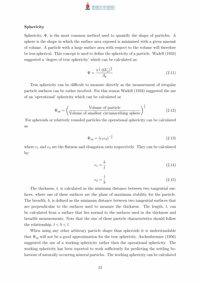
Sphericity
Sphericity, Ψ, is the most common method used to quantify the shape of particles. A
sphere is the shape in which the surface area exposed is minimised with a given amount
of volume. A particle with a large surface area with respect to the volume will therefore
be less spherical. This concept is used to define the sphericity of a particle. Wadell (1933)
suggested a ‘degree of true sphericity’ which can be calculated as:
Ψ =π
13 (6Vp)
23
Ap
(2.11)
True sphericity can be difficult to measure directly as the measurement of irregular
particle surfaces can be rather involved. For this reason Wadell (1933) suggested the use
of an ‘operational’ sphericity which can be calculated as
Ψop =
(Volume of particle
Volume of smallest circumscribing sphere
) 13
(2.12)
For spheroids or relatively rounded particles the operational sphericity can be calculated
as
Ψop = (e1e2)− 1
3 (2.13)
where e1 and e2 are the flatness and elongation ratio respectively. They can be calculated
by:
e1 =b
t(2.14)
e2 =l
b(2.15)
The thickness, t, is calculated as the minimum distance between two tangential sur-
faces, where one of these surfaces are the plane of maximum stability for the particle.
The breadth, b, is defined as the minimum distance between two tangential surfaces that
are perpendicular to the surfaces used to measure the thickness. The length, l, can
be calculated from a surface that lies normal to the surfaces used in the thickness and
breadth measurements. Note that the size of these particle characteristics should follow
the relationship, t < b < l.
When using any other arbitrary particle shape than spheroids it is understandable
that Ψop will not be a good approximation for the true sphericity. Aschenbrenner (1956)
suggested the use of a working sphericity rather then the operational sphericity. The
working sphericity has been reported to work sufficiently for predicting the settling be-
haviour of naturally occurring mineral particles. The working sphericity can be calculated
23

as
Ψw =12.8 (e1e2
2)13
1 + e2 (1 + e1) + 6√
1 + e22 (1 + e1
2)(2.16)
Although Wadell (1934) claimed that the sphericity can be used to correlate the drag
coefficient of a particle, Isaacs & Thodos (1967) reported that sphericity is inadequate
to describe drag flow even over smooth cylinders, not to mention irregular particles.
Sphericity has its uses such as to adjust for the particle diameter when working inside
a packed bed, or when a correlating parameter is necessary to describe creeping flow
past bodies that geometrically resemble spheres. But sphericity as a shape descriptor is
lacking when correlating particle drag for irregular particles (Thompson & Clark, 1991).
Despite the fact that the sphericity has these known drawbacks, it is a well known and
well understood shape descriptor, which would explain its popularity in elutriation rate
constant correlations.
Other particle shape descriptors
Circularity is for two dimensions what sphericity is for three dimensions. It is defined
as the ratio of the circumference of a sphere with the same cross-sectional area as the
particle cross section and the actual circumference of the particle cross section:
{ =πdeq
Particle circumference(2.17)
As can be seen from equation 2.17 the circularity of a particle should be calculated
from a two dimensional projection of a particle. This method is normally used in con-
junction with image processing, where a two dimensional photo of particles is obtained,
either with a camera or with a microscope, depending on the resolution required and the
size of the particles. The method with which the circularity of a particle is calculated
makes it a much easier method to use as a shape descriptor because it does not involve
the measurement of the entire surface area of the particle. Smolders & Bayens (1997)
used a circularity obtained from a microscope instead of a sphericity to calculate particle
terminal velocities.
A full review of the popular shape description techniques can be seen in appendix
A. These techniques include Heywood shape factors, Fourier descriptors, Fractal dimen-
sions, Polygonal harmonics, Piper’s angle and Delta analysis and Multi-scale roughness
descriptors. Of these techniques, the fractal dimensions, polygonal harmonics and Piper’s
angles, together with the circularity will be applied in this study to attempt to differen-
tiate between particle shapes.
In a study on liquid–solid fluidisation Flemmer et al. (1993) did a review on how
particle shape can influence the hydrodynamics of a single particle. It was found that
24

no well-accepted correlation exists that includes the effect of particle shape on hydrody-
namics for even single irregular particles, not to even mention mixtures of particles as
found in fluidised beds. In the study mentioned, Flemmer et al. (1993) went ahead to
study the modern techniques of particle shape description and how they might be used to
adjust for the effect of shape in fluidisation behaviour. The voidage during homogeneous
fluidisation was chosen as the parameter to test the effect of shape on. Although the
conclusions drawn can not be applied on a gas–solid fluidised bed, It does give a good
starting point for a study on the effect of particle shape on gas–solid fluidisation. Sookai
et al. (2005) did a study on different particle shapes, sizes and densities in gas–solid flu-
idisation. They found that particles with a high sphericity tend to entrain more readily
than particles with a low sphericity.
2.4 Modelling Entrainment and Elutriation
2.4.1 Entrainment flux
As stated previously, for particles to be transported into the freeboard and to be entrained
by the gas flowing out of the fluidised bed, they first have to be ejected into the freeboard
from the bed surface. The ejection of the particles into the freeboard is a complex process
(As all fluidised bed processes) of clusters, strands and single particles all accelerating,
decelerating, colliding with each other, separating from each other, etc. To be able to
describe this complex process, simplifying assumptions have been made to reduce the
process to three phases, or two entrainment flows. Both of these assumptions are reputed
to lead to similar results (Yang, 2003: p.124). But as the two phase description is easier
to understand, it will be explained here.
In short the entrainment flux flowing from the fluidised bed surface to the fluid outlet
can be divided into two streams – One stream of solids that are entrained and will flow
all the way to the fluid outlet to leave the bed and one stream of solids decreasing in
velocity until they fall back to the bed. This can be described as:
Eih = Ei∞ + Ei0 exp (−ai h) = xBiK∗
i∞ + Ei0 exp (−ai h) (2.18)
Therefore to calculate a value for the entrainment flux at a height between the bed
surface and the TDH, it is necessary to know the elutriation rate constant, K∗i∞, the
entrainment flux at the bed surface, Ei0, and the exponential decay coefficient, ai. Wen
& Chen (1982) stated that ai varies between 3.5 and 6.4m−1. A value of 4m−1 is recom-
mended in cases where little information is known about the system. Note that equation
2.18 reduces to elutriation rate constant at a height, h, equal to or higher than the TDH.
The entrainment flux at the bed surface can be calculated from having entrainment
25

fluxes at two different heights. Alternatively, one of the correlations in table 2.1 can be
used.
Table 2.1: Commonly used correlations to predict the entrainment flux at the fluidised bedsurface, E0
No Correlation Reference
1 E0 = 3.07× 10⁻⁹ Adb(U−Umf)0.25
ρ3.5g g0.5
µ2.5 Wen & Chen (1982)
2a Bubble nose model
E0 = 3dp(1−εmf)(U−Umf)
dbPemberton & Davidson (1986)
2b Bubble wake modelE0 = 0.1 ρs (1− εmf ) (U − Umf ) Pemberton & Davidson (1986)
3 E0 = 9.6 (U − Umf ) A db
(298Tb
)3.5
Choi et al. (1989)
2.4.2 Elutriation rate constant
The elutriation rate constant, K∗ih, is defined as the ratio of the instantaneous rate of
solid removal of the particle size, dpi, per unit cross sectional bed area, A, to the fraction
of the mass of bed material, XBi, with the particle size, dpi
(Yang, 2003: p.116). This
can be expressed mathematically as:
K∗ih =
Eih(t)
xBi(t)
(2.19)
with the entrainment flux, Eih, defined as:
Eih(t) =1
A
d
dt(xBi
(t)MB(t)) (2.20)
The elutriation rate constant is normally determined in batch experiments. To do
this the mass of solids captured over a time, t, have to be correlated with the elutriation
rate constant. This can be done by integrating equation 2.20. This will result in:
Mit = xBi0 MB
[1− exp
(−K∗
ih A
MB
)](2.21)
Note that the integration of equation 2.20 is only accurate when the mass of solids in
the bed, MB, does not change much with respect to time. The exponentially decreasing
26

concentration profile of solids in the freeboard is a well known occurrence (Kunii &
Levenspiel, 1991: p.177). Care should be taken therefore to know exactly what elutriation
is measured. If the elutriation is measured at a height below the Transport Disengagement
Height (TDH), it cannot be compared with the elutriation rate constant, K∗i∞ given by
most correlations.
The method by which elutriation is measured together with equation 2.18 explains
why the terms elutriation and entrainment are so often interchanged in literature. An
elutriation rate constant is used to predict an entrainment flux above the TDH. Therefore,
above the TDH, the elutriation rate and the entrainment flux is equal when doing a batch
experiment. This is because in a batch experiment all the entrained solids are removed
from the fluidised bed and can therefore be considered as elutriated solids. This fact
should be noted to ensure that one does not get confused by the interchangeability of
these terms in literature.
The elutriation rate constant is one of the parameters in fluidised beds that has the
most correlations to predict it, as it is so hard to determine from first principles due to
the complex and chaotic nature of the fluidised bed freeboard. A list of the most widely
used correlations can be seen in table 2.2. The earliest commonly used correlation is the
one determined by Zenz & Weil (1958). They considered the freeboard above the TDH
to behave like a pneumatic transport line at choking conditions. What this means is
that the freeboard above the TDH carries as much solids as is possible, before the solids
start to influence each other and start to increase the effective particle diameter. This
choking specification is commonly used in the description of pneumatic transport lines.
The entrainment flux above the TDH can therefore be calculated by dividing the bed
contents into a number of particle diameters, and calculating the choking load for each
of these diameters. The entrainment flux for each diameter can be calculated as:
Ei∞ = xBiGsi
(2.22)
With the entrainment flux for each particle diameter known, the total flux can be
calculated by adding all the fluxes together.
This method for calculating the total elutriation rate constant is most commonly used
in elutriation rate constant correlations, as can be seen in equations 2, 3, 4, 5, 6, 7, 10
and 11 in table 2.2. The biggest difference in the various correlations is the way in which
the choking loads and the particle size distributions are calculated (Yang, 2003).
27

Tab
le2.
2:C
omm
only
use
dco
rrel
atio
ns
for
the
Elu
tria
-
tion
rate
const
ant
K∗ i∞
No
Cor
rela
tion
U(m
/s)
D(m
)d
p(µ
m)
Ref
eren
ce
1K∗ i∞
gd2 pi
µ(U−U
t)2
=0.
0015
Re0
.6t
+0.
01R
e1.2
t0.
3-
1.0
0.07
-1.
010
0-
1600
Yag
i&
Aoch
i(1
955)
as
quot
edby
Lin
etal
.(1
980)
2K∗ i∞
ρf
U=
1.
26×
107
(U
2
gd
pi
ρ2 s
) 1.8
8
for
U2
gd
pi
ρ2 s
<3.
1
1.31×
104
(U
2
gd
pi
ρ2 s
) 1.1
8
for
U2
gd
pi
ρ2 s
>3.
10.
3-
0.7
0.05×
0.53
40-
200
Zen
z&
Wei
l(1
958)
3K∗ i∞
ρf(U−U
t i)
=1.
52×
10−5
( (U−U
t i)2
gd
pi
) 0.5
Re0
.725
0.6
-1.
00.
102
700
Wen
&H
ashin
ger
(196
0)
4K∗ i∞
ρf(U−U
t i)
=4.
6×
10−2
( (U−U
t i)2
gd
pi
) 0.5
Re0
.3( ρ
s−ρ
f
ρf
) 0.1
5
0.9
-2.
80.
031
-0.
067
700
-19
00Tan
aka
etal
.(1
972)
5K∗ i∞
ρf
U=
B+
130
exp
[ −10.
4( U
t i U
) 0.5
(U
mf
U−U
mf
) 0.2
5]
0.6
-2.
40.
91×
0.91
60-
1000
Mer
rick
&H
ighle
y(1
974)
wit
hB
=10−4
to10−3
6K∗ i∞
ρf
U=
23.7
exp
( −5.4
Ut i U
)0.
6-
3.0
0.07
660
-22
0G
eldar
tet
al.(1
979)
Con
tinued
onN
ext
Pag
e..
.
28

No
Cor
rela
tion
U(m
/s)
D(m
)d
p(µ
m)
Ref
eren
ce
7K∗ i∞
ρf
U=
9.43×
10−4
(U
2
gd
p
) 1.6
5
0.1
-0.
30.
61×
0.61
10-
125
Lin
etal
.(1
980)
58≤
(U
2
gd
p
)≤
1000
0<
dp
<74
µm
8K∗ i∞
=0.
011
ρs
( 1−
Ut i U
) 20.
9-
3.7
0.92×
0.92
300
-10
00C
olak
yan
&Lev
ensp
iel(1
984)
9K∗ i∞
=2.
8×
10−2
( U−U
t i
U
) 1.6
( ρs−ρ
f
ρs
) 0.5
4U
2.1
t iD
hK
ato
etal
.(1
985:
p.
134
-147
)as
quot
edby
Yan
g(2
003)
10K∗ i∞
ρf
U=
2.90
8(
U2
gd
p
) 3( ρ
f ρs
) 2( g
dp
gd
b
) 3Subbar
ao(1
986)
11K∗ i∞
ρf
U=
1.6(
U Ut i
) (1−
Ut i U
)Sci
azko
etal
.(1
991)
12K∗ i∞
=5.
4×
10−5
ρs
( U 0.2
) 3.4( 1−
Ut i U
) 20.
2-
0.7
30-
780
Bae
yens
etal
.(1
992)
for
dp≤
1.0
325×1
0−
2
ρ0.7
25
s
13K∗ i∞
=0.
35ρ
sU
A(1−
ε)H
0.1
-0.
60.
071
30-
200
Nak
agaw
aet
al.(1
994)
wit
h(1−
ε)H
=7.
41×
10−3
R1.8
7A
0.5
5H−0
.64
FB
0.08×
0.08
and
R=
Σx
i
( U−U
t i
Ut i
)fo
rU
t i<
U0.
15×
0.15
Con
tinued
onN
ext
Pag
e..
.
29

No
Cor
rela
tion
U(m
/s)
D(m
)d
p(µ
m)
Ref
eren
ce
14K∗ i∞
=
23
.7ρ
fU
2.5ex
p( −5
.4U
t i U
)fo
rR
e c<
3000
14.5
ρfU
2.5ex
p( −5
.4U
t i U
)fo
rR
e c>
3000
0.2
-0.
80.
076
and
0.15
217
-77
Tas
irin
&G
eldar
t(1
998)
15K∗ i∞
dp
µ=
Ga0
.5ex
p( 6.
92−
2.11
F0.3
03
g−
13.1
F0.9
02
d
)0.
3-
0.7
0.06
-1.
150
-10
00C
hoi
etal
.(1
999)
wit
hF
g=
gd
p(ρ
s−
ρf)
Fd
=C
dρ
fU
2
2
30

Another commonly used assumption is to calculate the flux of solids from the dense
bed into the freeboard by using bubble properties, such as size, velocity, etc. This method
has been used by Smolders & Bayens (1997) and George & Grace (1978) as quoted by
Yang (2003). The problem with this method is that it is assumed that the flux above
the TDH is only that of the particles with a terminal velocity less than the fluid velocity
in the freeboard. This is known to be inaccurate from experimental investigations, as
stated in section 2.2.2.
Most of the other correlations (Equations 1, 8, 9, 12, 13, 14 and 15 in table 2.2) for
the elutriation rate constant are empirically fitted models with little or no theoretical
basis.
When any of the correlations listed in table 2.2 are used, care should be taken so
that the correlation is chosen for a system similar to that on which the correlation was
developed, as these correlations can differ significantly. This significant difference can be
seen in figure 2.15. Note that most of the correlations predict values within a factor 100
of each other. But some of the correlations differ more than a factor 106.
0.7 0.8 0.9 1 1.110
−6
10−5
10−4
10−3
10−2
10−1
100
101
102
103
104
Linear velocity (m.s−1)
Elu
tria
tion
rate
con
stan
t (kg
.m−
2 .s−
1 )
Yagi & Aochi (1955)Zenz & Weil (1958)Wen & Hashinger (1960)Tanaka et al.Merrick & Highley (1972)Geldart et al. (1979)Lin et al. (1980)Colakyan & Levenspiel (1984)Kato et al. (1985)Subbarao (1986)Sciazko (1991)Bayens et al. (1992)Nakagawa et al. (1994)Tasirin & Geldart (1998)Choi et al. (1999)
Figure 2.15: Comparison between the different correlations for the elutriation rate constantK∗
i∞ (Numbers in legend refers to correlation number as used in table 2.2)
To better understand these correlations and when necessary, make small modification
to these correlations to better fit a specific system, the principles, or pseudo-principles
behind these equations has to be understood properly. Dimensionless groups are mostly
used as dimensional analysis makes it easier to develop empirical correlations. Even
though the dimensionless groups can be completely meaningless in some cases, most
of the time the groups have some physical representation which is associated with the
entrainment process. These groups are:
31

• K∗i∞/ρf U, used in all of the correlations based on the pneumatic transport line
method, is the ratio of the solids mass flux and the gas mass flux
• U2/gdp, also known as the Froude number (Fr), is the ratio between the inertial force
on the particles and the gravity force on the particle
• U −Uti can be used in place of the superficial velocity U . This is known as the slip
velocity which is a direct indication of how much higher the superficial velocity is
than the terminal velocity for a specific particle size. It is therefore a measure of
how quickly a particle can be removed from the freeboard. The problem with using
a slip velocity is that the slip velocity implies that only particles with a terminal
velocity below the superficial velocity of the gas in the freeboard are entrained,
which have been proved incorrect as mentioned in section 2.2.2
• Uti/U is another way to represent the slip velocity that allows for particles with a
terminal velocity higher than the freeboard superficial velocity to be entrained
• The Reynolds number (Rep) is also used in some correlations as an additional
velocity term together with the slip velocity and the Froude number
• ρf/ρs or ρs − ρf/ρf is a density ratio, which is used to adjust for the density effects
such as a denser gas, or heavier particles.
As figure 2.14 indicated, the terminal velocity of a particle is decreased when the
sphericity is reduced. This implies that less spherical particles should have a higher
entrainment rate if the hydrodynamics can be described by the behaviour of a single
particle. Figure 2.16 shows how some of the correlations in table 2.2 quantifies the effect
of particle shape on entrainment rate for similar sized particles. According to these
models, particle shape should therefore have an effect on the entrainment rate. However,
no study has been found in literature where all the particle properties, except for particle
shape, has been kept constant to verify whether any of the models are applicable to
include the effect of particle shape, and more importantly is it sufficient to only adjust
the coefficient of drag for a single particle with a sphericity to include the effect of particle
shape on entrainment.
2.5 Concluding remarks
Entrainment is a well known occurrence in fluidised beds and in many cases, entrainment
is considered to be problematic, as the loss of solids from the bed is responsible for ad-
ditional costs. The process of entrainment is still not very well understood and many of
the factors that influence entrainment are correlated empirically instead of phenomeno-
logically or fundamentally. Important factors are therefore lumped in empirical constants
32

0.1 0.2 0.3 0.4 0.5 0.6 0.7 0.8 0.9 10
0.1
0.2
0.3
0.4
0.5
0.6
0.7
0.8
0.9
1
Sphericity
Rat
io o
f ent
rain
men
t rat
es
Merrick & Highley (1972)Geldart et al. (1979)Choi et al. (1999)
Figure 2.16: The ratio of entrainment rates for different sphericities, where the ratio is definedas: Entrainment rate of particles with a sphericity of 1
Entrainment rate of particles with a sphericity of the value on the x-axis
from time to time, which would explain why there is such a large deviation in the values
predicted for the elutriation rate constants. One factor that is left out in most cases is
the shape of the solids. It is true that the shape of the solids is taken into consideration
when calculating the terminal velocity of the solids, but when studying the literature on
elutriation rate constant correlations, little information is given on how a sphericity, if
at all, was determined. The purpose of this study is to evaluate how shape can influence
the entrainment rate of solids and to see how different shape characterisation techniques
report different shape factors. This will be done by using two particle mixtures with
identical properties except for the particle shapes in entrainment tests. There is also a
shortage of information in literature on how heavier particles behave in fluidisation. This
study is aimed at helping to understand the entrainment behaviour in high tempera-
ture Fischer-Tropsch (HTFT) reactors better. These reactors use an iron based catalyst,
which is exactly the type of solid on which fluidisation behaviour is scarce.
33

CHAPTER 3
Experimental
3.1 Experimental Setup
3.1.1 Materials
The solid packing used in the fluidised bed was Ferrosilicon (FeSi) obtained from BHP-
Billiton. Two types of FeSi were used, atomised FeSi and milled FeSi. Both the atomised
and the milled FeSi are non-porous. A mixture of 50% atomised and 50% milled FeSi
by mass was also used. A description of these solids can be seen in table 3.1. A sample
Table 3.1: Properties of particle mixtures used inside fluidised bed reactor
Property Atomised FeSi Milled FeSi Mixture
Volume weightedmean particle 38.44µm 49.96 µm 41.78 µm
diameter
Solid density 6690 kg/m3 6589 kg/m3 6621 kg/m3
Solid packing density 3753 kg/m3 3490 kg/m3 3630 kg/m3
Geldart classification A-B A-B A-B
Particle shape Spherical Irregular Both irregular and spherical
of how the atomised and the milled FeSi differ in appearance can be seen in figure 3.1.
The FeSi was chosen as the solid to be fluidised since the FeSi is very similar in physical
34

(a) A scanning electron microscope image of theatomised FeSi
(b) A scanning electron microscope image of themilled FeSi
Figure 3.1: A comparison of the difference in appearance between the atomised and the milledFeSi
properties to the high temperature Fischer-Tropsch (HTFT) catalyst. Both the FeSi and
the HTFT catalyst lies on the Geldart A-B boundary, which causes the solids to have
both Geldart A and Geldart B behaviour.
The densities of the FeSi mixtures were determined by measuring the displacement
of water by a certain mass of solids. Care was taken to ensure that only the solids are
responsible for displacing the water and that no air bubbles were trapped along with
the solids. The packing densities of the mixtures were determined for a tightly packed
mixture, as this was the state in which the solids were found in the dipleg where the
entrainment measurements were made.
3.1.2 Equipment
All tests were done in a 140mm perspex column, with a height of 5.5m. A schematic
diagram of this experimental setup can be seen in figure 3.2. Air, supplied by a BSC15
Evolution Fini Compressor (SC-1 in the diagram), was used as the fluidising medium.
The flow rates to the fluidised bed and the cyclone were measured by the flow meters FT-
2 and FT-1 respectively, which were both HO11/4X11/4-20-CB-1MC3PA-NTP-X Hoffer
turbine flow meters. These flow meters are reported to have an accuracy of 0.25% and are
able to measure flow rates of 5 to 100 actual cubic meters per hour with a 1% linearity,
which means that a high level of precision can be expected. The pressure drop was
measured over various sections of the setup with Rosemount 3051 differential pressure
transmitters. The detail for each transmitter can be seen in table 3.2. All of the above
mentioned instrumentation has 4 - 20 mA analog output signals, which were recorded on
a Datataker DT500 series 3. The data of all the instrumentation could then be extracted
35

FB-1 : Fluidised bed DPT-4 : Differential pressure cellPC-1 : Plenum chamber PR-1 : Pressure regulator SC-1 : Compressor FT-1 : Turbine flow meterCC-1 : Cyclone FT-2 : Turbine flow meterBF-1 : Bag Filter BV-1 : Ball valveDL-1 : Dip leg for solids return BV-2 : Ball valveDPT-1 : Differential pressure cell BV-3 : Ball valveDPT-2 : Differential pressure cell NV-1 : Needle valveDPT-3 : Differential pressure cell
FT-2BV-3
BV-1NV-1BV-2
SC-1PR-1
BF-1
FT-1DPT-1DPT-2DPT-3
DPT-4
PC-1FB-1 DL-1
CC-1
Figure 3.2: A schematic of the experimental setup used for all the tests
from the Datataker into a spreadsheet.
A chiller was used to maintain the air temperature at 15 °C at all times, while the
pressure regulator, PR-1 as seen in figure 3.2, was used to maintain the fluidised bed
pressure at 15 kPag. With temperature and pressure constant, as well as all the other
factors verified, it is possible to measure only the effect of particle shape on entrainment
rate.
3.2 Method
The fluidised bed is a chaotic system and small disturbances can therefore cause a major
deviation in the operating point of the bed. It is therefore important to ensure that the
values are measured under the same conditions.
Prior to every set of experiments, the bed was packed with about 30 kg of FeSi. This
36

Table 3.2: Detail information of differential pressure drop transmitters
Label in figure 3.2 Range Accuracy Function
DPT-1 0 - 63 kPa 0.1% Measure gas distributor pressure drop
DPT-2 0 - 63 kPa 0.1% Measure dense bed pressure drop
DPT-3 0 - 63 kPa 0.1% Measure freeboard pressure drop
DPT-4 0 - 63 kPa 0.1% Measure cyclone pressure drop
was done to ensure that even at the highest entrainment rate, the loss of solids from the
bed will be less than 20% of the total bed mass, as suggested by Kunii & Levenspiel
(1991: p.176) for batch experiments.
3.2.1 Minimum fluidisation measurements
The minimum fluidisation velocity of a fluidised bed should give an indication of what
the morphology of the bed is like. How the particles pack together in a fluidised bed
will be affected by the shape of these particles. To measure the minimum fluidisation
velocity, the bed was first fluidised at a higher velocity after which the ball valve, BV-1,
was shut quickly to ensure that the bed is in a loosely packed state. All the excess gas
in the bed was then allowed to escape over a period of 10 minutes, so to ensure that
the true minimum fluidisation velocity is measured. BV-1 was opened again, after the
needle valve, NV-1, was closed completely. NV-1 was then opened a small fraction and
the pressure drop over the bed was recorded from the differential pressure transmitter,
DPT-2. After the pressure drop measured by DPT-2 stabilised to a constant value, NV-1
was opened a fraction more. This process was repeated until the bed started bubbling.
The pressure drop profile as a function of the linear velocity can then be used to calculate
the minimum fluidisation velocity. This techniques is a common method to measure the
minimum fluidisation velocity as can be seen in the work of Chitester et al. (1984) and
Adanez & Abanades (1991), where the minimum fluidisation velocity is read off at the
inflection point on the pressure drop profile.
3.2.2 Entrainment measurements
Entrainment rates were measured at five different flow rates. A list of the operating
conditions of the fluidised bed can be seen in table 3.3. The cooled down air naturally
has a low moisture content as a result of the cooling process. The low humidity together
37

Table 3.3: Operating conditions used for the fluidised bed
Flow rate 0.17 m/s 0.24 m/s 0.32 m/s 0.38 m/s 0.43 m/s
Condition
Pressure 102 kPaa 102 kPaa 102 kPaa 102 kPaa 102 kPaa
Temperature 15 °C 15 °C 15 °C 15 °C 15 °C
with the material used for the column, and the type of solids used resulted in a high
charge of static electricity forming on the column walls. To counter act this, a copper
wire was wound around the column, with special focus on the dipleg in which the solids
from the cyclone are returned to the dense bed. This resulted in the column being well
earthed which caused less solids sticking to the column side and less static shocks for
the masters student. The air to the fluidised bed was opened by opening ball valves,
BV-1 and BV-2. Then the needle valve, NV-1, was used to control the air flow rate
into the fluidised bed at the specified value. The fluidised bed was then left to reach a
steady state to ensure that only the entrainment rate was measured and not the fluidised
bed dynamics. Steady state is defined as the point where the solids level in the dip-leg
remains constant. When this state is reached, the ball-valve, BV-3, is closed to capture
the entrained solids – which under normal conditions are returned from the cyclone via
the dip-leg to the bed. The fluidised bed is operated with ball-valve BV-3 closed for a
set period of time, after which the air flow into the fluidised bed is stopped by closing
ball-valves BV-1 and BV-2. The dip-leg is then tapped to ensure that the packing of the
solids inside the dip-leg can always be considered to be in a ‘tightly packed’ state. This is
also the packing state for which the bulk densities of the FeSi was measured. The height
of the tightly packed solids above BV-3 is then measured to calculate the mass of solids
removed from the bed due to entrainment.
3.2.3 Repeatability
The chaotic nature of the fluidised bed have been mentioned and the effect of this on
experimental measurements should be obvious. It is therefore necessary to ensure that
the experimental setup has a sufficiently good repeatability. This was done by loading the
bed with a batch of solids and measuring the entrainment rate, after which the bed was
drained and the following type of solids was loaded and the entrainment was measured.
This was done for all three the solid mixtures. After all three solids were tested, the
process was repeated again. The repeatability of the experimental setup can be seen in
table 3.4. Note that the average values of the entrainment rate for the different particle
38

mixtures are used as the benchmark against which the measured values are checked, as
can be seen in equation 3.1.
AARE =n∑i
|Entrainment rateAverage − Entrainment rateMeasured|Entrainment rateAverage
1
n× 100 (3.1)
When studying these errors, it can be seen that size the experimental error is far from
Table 3.4: Relative errors in entrainment for different particle mixtures with respect to theaverage value of entrainment for the different particle mixtures
Solids mixture AARE Maximum
Atomised FeSi 14.28% 40.19%
Milled FeSi 18.72% 32.99%
FeSi Mixture 3.77% 20.12%
ideal, however, errors, of this size, in the few cases where errors are shown, are frequently
found in literature on entrainment data (Merrick & Highley, 1974; Geldart et al., 1979;
Lin et al., 1980).
3.2.4 Procedure verification
To ensure that particle shape is the only effect being studied, some tests had to be done
to verify that the other factors described in chapter 2 are kept constant for all three
particle mixtures used.
Particle size distribution
All the information on the size of the particles used was obtained with a Malvern Mas-
tersizer 2000. The Malvern uses laser diffraction to measure the particle size distribution
of a sample. The particle size measured by the Malvern is a volume mean diameter.
The particle size has a significant effect on the entrainment rate, as already mentioned
in section 2.3.3. For particles below the critical particle diameter, the entrainment rate
of that particle size can be assumed to be the same value as that of the critical particle
diameter. For FeSi, this critical diameter is ±17µm. A comparison of the particle size
distributions can be seen in figure 3.3. This figure gives a good indication that the all
the particle mixtures should behave similarly as a result of the particle diameter. All the
mixtures contains a significant fraction of fines, a comparison of the percentage of fines
39

100
101
102
103
0
0.05
0.1
0.15
0.2
0.25
Particle diameter (µm)
Fra
ctio
n of
tota
l sam
ple
Atomised FeSiMilled FeSiFeSi mixture
Figure 3.3: A comparison for the particle size distribution for all three mixtures used
in the different mixtures can be seen in table 3.5. Note that fines are defined as solids
with a particle size of less than 17 µm.
Table 3.5: Fines fraction of different particle mixtures
Particle mixture Percentage fines
Atomised FeSi 8.57%
Milled FeSi 1.78%
FeSi mixture 5.51%
Attrition
One of the negative influences of entrainment is that the particles tend to break up into
smaller particles inside the cyclone as a result of the high collision rate and high linear
velocities inside the cyclone as well as a lot of friction between the particles and the cyclone
(Yang, 2003: p.207). This attrition may create a large amount of fines which cannot be
removed by the cyclone and are lost inside the filters. To ensure that significant attrition
does not occur inside the experimental setup, a comparison has to be done between fresh
40

unused solids and spent solids after a long period of operation (More than a week of
experimental time, or 24 hours time on stream). This can be seen in figure 3.4. The
100
101
102
103
0
0.02
0.04
0.06
0.08
0.1
0.12
0.14
0.16
0.18
Particle diameter (µm)
Fra
ctio
n of
tota
l sam
ple
Fresh atomised FeSiSpent atomised FeSi
(a) The effect of attrition due to extensive en-trainment on atomised FeSi
100
101
102
103
0
0.05
0.1
0.15
0.2
0.25
Particle diameter (µm)
Fra
ctio
n of
tota
l sam
ple
Spent milled FeSiFresh milled FeSi
(b) The effect of attrition due to extensive en-trainment on milled FeSi
Figure 3.4: Indication of how the PSD’s of the FeSi mixtures change after an extended periodinside the fluidised bed
PSD’s inside the fluidised bed rapidly moved towards that of the spent FeSi profiles seen
in the figure. It was therefore assumed that the PSD’s in the fluidised bed at all times
were that of the spent FeSi profiles. The combination mixture is made up of atomised
and milled FeSi and for that reason the attrition effect was not tested on the combination
mixture, as no significant attrition was found in either the atomised or the milled FeSi.
Note that the mass of the filters were measured from time to time to know how much fines
were lost in the cyclone. Care was taken therefore that the amount of fines captured in
the filters were insignificant and that the entrainment measurements were not influenced.
Bed height
As noted in section 2.3.1, the height of the packed bed can influence the entrainment
rate. The term ‘deep bed’ is often used when speaking of Geldart A powders, where the
depth of the fluidised bed is sufficient so that a stable bubble size have been reached and
a further increase in bed height will not influence the bubble properties. To ensure that
a ‘deep bed’ is being used a batch of experiments were done with three different packed
bed heights, namely 0.4m, 0.6m and 0.8 m. Bed heights of double the normal packing
height, one and a half times the normal packing height and the normal packing height
(0.4m) were compared with each other. The results of these comparisons can be seen in
table 3.6. The absolute average relative difference was used to compare the entrainment
rates of the different bed heights and was calculated as:
41

AARD =n∑i
|Entrainment rate0.4m − Entrainment rateCompared height|Entrainment rate0.4m
1
n× 100
These relative differences associated with the difference in bed heights are rather small
Table 3.6: Relative difference in entrainment for different fixed bed heights with respect to theaverage value of entrainment at the normal fixed bed height
Solids mixture Error compared to average values1.5 × normal height 2 × normal heightAARD Maximum AARD Maximum
Atomised FeSi 23.47% 40.19% 8.62% 18.02%
Milled FeSi 14.94% 24.18% 20.79% 26.55%
FeSi Mixture 7.76% 15.6% 4.92% 7.58%
when compared with the repeatability results seen in table 3.4. Therefore it can be said
with confidence that the bed depth of 0.4 m is sufficient to consider the fluidised bed as
a deep bed.
3.3 Image Processing
Most shape characterisation techniques relies on the availability of an image of the par-
ticles so that the features used in shape characterisation can be measured. It is therefore
necessary to have an image with a high enough resolution of the particle in question
to be able to measure these features. The choice had to be made between using either
a scanning electron microscope (SEM), or a normal light microscope with an attached
camera. The light microscope is cheaper and easier to use but the depth of field that it
can focus on at any time is very shallow. This results in the problem that only a section
of the particle under investigation will be visible. The SEM is much more cumbersome to
use and expensive, but it has a much deeper depth of field in focus. A comparison of the
images that the two microscopes can take can be seen in figure 3.5. The light microscope
is able to show detail inside the perimeter of the particle but the area of interest for
image processing is the perimeter of the particle. The perimeter of the particles in the
light microscope images are rather smudged. The perimeters of the particles in the SEM
images are properly in focus. With the detail in these images, a true representation of
the particle perimeter can be obtained. The three dimensional nature of the particles
42

(a) Image of atomised FeSi particles as taken withlight microscope
(b) Image of milled FeSi particles as taken withlight microscope
(c) Image of atomised FeSi particles as taken withSEM
(d) Image of milled FeSi particles as taken withSEM
Figure 3.5: Comparison between the quality of the images taken with the two types of micro-scopes
can also be seen in the SEM images, although it cannot be quantified with normal image
processing techniques. With this extra ability, an additional, qualitative observation can
be made of the differences between the two mixtures. The atomised particles tend to
be mostly round, in other words all three dimensions are of a similar size. The milled
particles appear to be mostly flakes, which means that two of the three dimensions are
much larger than the third. This observation can not be made with a light microscope.
These images therefore show how the light microscope is insufficient for the type of im-
ages required for shape description by image processing. The SEM used to capture all
the images was a JEOL JSM-6300 Scanning Microscope.
To be able to do particle shape analysis with the images obtained from the SEM,
these images had to be processed and manipulated in such a way that the particles are all
available in Matlab as datasets which can then be processed further. The whole process
of obtaining the particle data from the images as well as the consequent processing to
43

analyse the particle shapes are explained in detail in appendix B.
44

CHAPTER 4
Results and discussion
4.1 Fluidisation characteristics
4.1.1 Minimum fluidisation
The minimum fluidisation velocity of a fixed bed can give a good indication of the internal
structure of the bed. The minimum fluidisation velocity was measured by measuring the
pressure drop over the fixed bed up to the point of fluidisation. The results of these
measurements can be seen in figure 4.1. These results show that a much larger drag on
0 1 2 3 4 5 6 70
5
10
15
Linear velocity (mm.s−1)
Pre
ssur
e dr
op o
ver
bed
(kP
a.m
−1 )
Umf
(a) Pressure drop profile over the fixed bed for theatomised FeSi (Umf = 6 mm/s )
0 2 4 6 8 10 12 140
5
10
15
20
25
Linear velocity (mm.s−1)
Pre
ssur
e dr
op (
kPa.
m−
1 )
Umf
(b) Pressure drop profile over the fixed bed forthe milled FeSi (Umf = 11 mm/s )
Figure 4.1: Results of the minimum fluidisation velocity measurements for both the atomisedand milled FeSi
the milled FeSi particles are required to overcome the gravitational and cohesive forces
between the particles and fluidise the bed. Since the densities of both the atomised and
the milled FeSi are the same, the reason for this higher energy requirement for fluidisation
45

has to be either the terminal velocity of the milled FeSi or the cohesive forces between
the milled FeSi particles, or a combination of these two effects. Note that the slightly
higher pressure drop for the atomised FeSi can be attributed to a lower voidage in the
bed, because as can be seen in table 3.1, the packing density of the milled FeSi is lower
than that of the atomised FeSi. The increased pressure drop can also be caused by more
frictional drag on the atomised FeSi compared to the milled FeSi, or the more likely
explanation, the more tortuous pores inside the atomised FeSi fixed bed result in longer
paths for the gas to flow through, which causes the higher pressure drop.
4.1.2 Solids entrainment
The results of the comparison between the entrainment rates for all the particle mixtures
can be seen in figure 4.2. It is quite obvious that the atomised FeSi has a significantly
0.15 0.2 0.25 0.3 0.35 0.4 0.4510
−2
10−1
100
Linear velocity (m.s−1)
Ent
rain
men
t rat
e (k
g.m
−2 .s
−1 )
Atomised FeSiMilled FeSiFeSi Mixture
Figure 4.2: Comparison of the entrainment rates for the different solid mixtures. Solid linesrepresent the average values for the individual mixtures
higher entrainment rate than the milled FeSi. To quantify this difference, on average the
entrainment rate for the atomised FeSi is about six times higher than that of the milled
FeSi.
The effect of the different fines concentrations
It is important to remember that this big difference in entrainment rates might be as
a result of the higher fines concentration in the atomised FeSi, as seen in table 3.5. In
attempt to disprove that the difference in fines concentration is only reason why the
entrainment rates of the mixtures differed, a third mixture of FeSi was made up. This
46

mixture contained 50% atomised and 50% milled FeSi by mass. If the increased entrain-
ment rate was caused only by the difference in particle size distribution, the mixture
should have an entrainment rate which is exactly halfway between the atomised and the
milled FeSi. Therefore, if a graph is constructed where the entrainment rate is plotted
as a function of the fraction atomised FeSi in the mixture, a straight line should be seen
between the milled FeSi (fraction atomised FeSi = 0) and the atomised FeSi (fraction
atomised FeSi = 1). To illustrate this better, theoretical mixtures of FeSi were made up
from the atomised and milled FeSi PSD’s ranging from an atomised FeSi fraction of 0.1
to an atomised FeSi fraction of 0.9. Together with the actual PSD’s of the milled and
the atomised FeSi, these theoretical mixtures were used to predict the elutriation rate
constant with the correlation developed by Geldart et al. (1979). The results of these
predictions can be seen in figure 4.3. A sphericity of 1 was used to calculate the terminal
0 0.1 0.2 0.3 0.4 0.5 0.6 0.7 0.8 0.9 10
0.02
0.04
0.06
0.08
0.1
0.12
0.14
0.16
0.18
Fraction of atomised FeSi
Pre
dict
ed e
ntra
inm
ent r
ate
(kg.
m−
2 .s−
1 )
U = 0.17 m.s−1
U = 0.24 m.s−1
U = 0.32 m.s−1
U = 0.38 m.s−1
U = 0.43 m.s−1
Figure 4.3: Prediction of how the entrainment rate should vary as the fraction of atomisedFeSi in a FeSi mixture changes according to Geldart et al. (1979).
velocities of the solids, therefore the results are not influenced by shape, but will only
predict the resultant effect of mixing two different mixtures with two different PSD’s on
entrainment rate. Assuming that the correlation of Geldart et al. (1979) is accurate, the
straight line relationship seen in figure 4.3 proves that if two mixtures of equal densities
but with different PSD’s are mixed, the entrainment rate is linearly dependent on the
fractions of the two mixtures. Therefore, if the higher entrainment rate of the atomised
FeSi compared to the milled FeSi as seen in figure 4.2 are caused by the difference in par-
ticle size only, a straight line relationship should be seen between the entrainment rates
of the three different experimental mixtures and the fraction of atomised FeSi present in
the mixtures. The measured relationship can be seen in figure 4.4. The results shown
47

0 0.2 0.4 0.6 0.8 10
0.2
0.4
0.6
0.8
1
1.2
1.4
1.6
1.8
Fraction of atomised FeSi
Ent
rain
men
t rat
e (k
g.m
−2 .s
−1 )
0.17 m.s−1
0.24 m.s−1
0.32 m.s−1
0.38 m.s−1
0.43 m.s−1
Figure 4.4: Experimental results of how entrainment rates vary as a function of the fractionof atomised FeSi in the solid mixture. Straight lines represent the theoreticalrelationships where the PSD is the only factor that influences the entrainmentrates.
are a good indication that the difference in the PSD’s for the atomised and the milled
FeSi are not solely responsible for the difference in entrainment rates, but that another
factor, namely particle shape, has to play a role.
4.2 Shape analysis results
From the SEM photos seen in section 3.3 there appears to be a very big difference in
particle shapes of the different mixtures. It is therefore necessary to see if it is possible
to quantify the difference in shape between the different solids. Most of the techniques
described in appendix A were used to quantify the difference in shape between the atom-
ised and the milled FeSi mixtures. The performance of the techniques can be seen in
table 4.1. Note that the absolute relative difference was calculated as:
ARD =|Value of shape descriptorAtomised − Value of shape descriptorMilled|
Value of shape descriptorAtomised
× 100 (4.1)
Of all the shape description techniques tested, only the circularity had the ability to
distinguish properly between shapes of the different particle mixtures. Therefore only
the circularity will be discussed in this section.
48

Table 4.1: Comparison between the performance of the different shape description techniques
Shape descriptor Absolute relativedifference
Circularity 9.08%
Fractal dimension 0.79%
Piper’s angle 0.33%
Persistence of 2nd harmonic 2.53%
Persistence of 3rd harmonic 3.96%
Persistence of 4th harmonic 0.10%
Persistence of 5th harmonic 0.39%
4.2.1 Circularity
Although sphericity for such small particles is difficult to measure with normal techniques
(Thompson & Clark, 1991), the circularity is a very easy parameter to measure if two
dimensional images of a particle is available. Circularity can be calculated by using the
surface areas of the particle projections as well as their perimeter length. The perimeter
of a circle with the same surface area as that of the particle under investigation can then
be calculated and compared to the known perimeter. A comparison of the circularity
for both mixtures can be seen in figure 4.5. It can be seen that both mixtures have
a relatively wide distribution in circularities, with the distribution of the atomised FeSi
shifted closer to a circularity of 1. Both mixtures have a large fraction of relatively circular
particles though, which can disqualify circularity as a good shape descriptor since it does
not distinguish between the different mixtures well enough. Note that most of the milled
FeSi particles are lying in their most stable position, which can make them appear more
spherical than they are.
4.2.2 Other techniques
The big overlap in circularities for the atomised and the milled FeSi indicated the need for
another shape characterisation technique that can distinguish better between the different
particle shapes. However, the performance of all the other techniques in appendix A
were shown in table 4.1 where it was indicated that circularity performed the best in the
49

0.4 0.5 0.6 0.7 0.8 0.9 10
0.01
0.02
0.03
0.04
0.05
0.06
Circularity
Nor
mal
ised
freq
uenc
y
AtomisedC
avg = 0.782
MilledC
avg = 0.711
Figure 4.5: The circularity of both the atomised and the milled FeSi as a frequency plot. {avg
for the atomised FeSi = 0.782 and {avg for the milled FeSi = 0.711
techniques tested. A more complete display of these results as well as a discussion of the
results for these other shape descriptors can be seen in appendix C. The problem with
most of the techniques in literature is that they characterise a particle shape based on a
two dimensional image. This can be accurate, but it can also mislead one into believing
that a particle is a sphere, when it is actually a thin disk. However, due to the lack of
anything better, the particle circularity will be used as the shape descriptor of choice in
this study. As is done in literature (Smolders & Bayens, 1997), the circularity will be
used in the same way as a sphericity. This means that in the drag coefficient correlation
(Equation 2.10), the sphericity will simply be replaced with the circularity. This has to
be done, as no other proper shape descriptor is available.
4.3 Understanding particle shape effects in entrain-
ment
The entrainment rate is definitely influenced by the shape of the particles that is fluidised,
as was shown in this chapter. How this occurs can possibly be explained by one or more
of the following ideas:
• The way the particle orientates itself as the gas flows over it can significantly affect
the terminal velocity of the particle
• The orientation of particles can influence the direction into which particles shoot
50

off after a collision between two particles.
• The Van der Waals forces between the particles are affected by the particle shape
Isaacs & Thodos (1967) reported that cylinders orientate themselves differently when
settling in water, depending on the ratio between the diameter and the length of the
cylinder. This behaviour have been attributed to the formation of vortexes around and
behind the cylinders which then induces secondary forces on the cylinders. This type
of behaviour is also possible in the fluidised bed. Particles like the milled FeSi, which
are flaky in nature, can orientate themselves in such a way that the coefficient of drag is
minimised and that they require a larger gas flow rate to keep them entrained. However,
this is hard to proof directly, as the particles are extremely small, and would therefore
require a special setup that includes a microscope to see how they orientate themselves
at different flow rates. However, the behaviour of a lot of particles together in a fluid
and a single particle in a fluid can hardly be assumed to be similar. The large amount
of collisions found inside the freeboard of a fluidised bed will in all likelihood cancel out
any effects that particle shape will have on the orientation of a particle in the freeboard.
When a sphere drifts in the fluidising air and another sphere collides with the sphere,
the direction into which the sphere shoots off is not influenced by the orientation of
the sphere. This happens because the centre of mass of a sphere is the same distance
from every point on the surface of that sphere. However, when a non spherical particle
is collided with, the direction into which the particle shoots off is a function of the
orientation of the particle. This means that when another particle collides with the
corner of a flake-like particle, the particle might veer off into a different direction since
the particle impact caused the particle to rotate around its centre of mass. What all of
this boils down to is that more spherical particles have a larger probability to have elastic
collisions while non-spherical particles tend to have less elastic collisions. However, this
is a lot of speculation and needs to be investigated further before any further statements
can be made.
Baeyens et al. (1992) as well as Ma & Kato (1998) noted that the Van der Waals forces
between a sphere and a plane is larger than the Van der Waals forces between two spheres.
This is as a result of the centres of mass of the two objects being able to move much closer
together. The shape of the milled FeSi, which is flaky, can therefore allow for much larger
Van der Waals forces between the particles. This will in turn result in a larger number
of clusters forming that will reduce the entrainment rate, as clusters tend to fall back to
the bed, while single particles are entrained and removed from the freeboard. If shape
affects the inter-particle forces, one would expect the more spherical particles to entrain
quicker and at lower velocities with the less spherical particles only getting entrained
at higher velocities where the momentum of the particles is sufficiently large enough to
overcome the Van der Waals forces. Proof of this theory is given in figure 4.6. This
51

0.15 0.2 0.25 0.3 0.35 0.4 0.450.66
0.68
0.7
0.72
0.74
0.76
0.78
0.8
0.82
0.84
Linear velocity (m.s−1)
Ave
rage
circ
ular
ity o
f en
trai
ned
solid
s sa
mpl
e
Atomised FeSiMilled FeSi
Figure 4.6: Illustration of how the average circularity of entrained solids change as the linearvelocity at which they were entrained increases
Par
ticle
circ
ular
ity
Particle diameter (µm)
0.95
0.9
0.85
0.8
0.75
0.7
0.65
0.6
0.55
0.50 7.67 15.34 23 30.67 38.34 46 53.67 61.34 69
0.005 0.01 0.015 0.02 0.025 0.03 0.035 0.04 0.045
Figure 4.7: An indication of how the particle circularity is distributed as a function of parti-cle diameter (Data from sample of atomised FeSi particles). Contours representnormalised frequencies. Note the high circularity of the small particles.
52

figure shows how the average circularity of the entrained particles changes as the velocity
with which the particles are removed from the bed increases. For the atomised FeSi, no
clear trend can be seen, as the difference in circularity is within experimental error. This
can be explained by the large amount of highly circular atomised FeSi particles of the
size fraction that gets entrained, as seen in figure 4.7. However, the milled FeSi shows
a clear trend. At low velocities the particles with high circularities, i.e. those that do
not form clusters as easily, are entrained and removed from the freeboard. As the gas
velocity increases, the momentum of the individual particles in the cluster are sufficiently
large enough to escape the clusters. The speed at which clusters collide with each other
and the reactor walls are also large enough to cause break-up of the clusters or ejection
of some of the particles in the clusters.
4.4 Predicting entrainment rates
In order to see which of the popular elutriation rate constants performs the best in
predicting the behaviour of the FeSi mixtures, all of the correlations were compared to
the experimental results. The ability of these models to include the effect of particle
shape should also be evaluated. As circularity is the shape descriptor with the best
performance in differentiating between the particle shapes of the different mixtures, it
will be used instead of a sphericity to adjust for the particle terminal velocity where
applicable. The performance of these correlations can be seen in table 4.2. Note that the
AARE is defined in this case as:
AARE =n∑i
|Entrainment rateMeasured − Entrainment ratePredicted|Entrainment rateMeasured
1
n× 100 (4.2)
The poor performance of all the different correlations in predicting the entrainment
rates for the mixtures once again shows the extreme importance in doing actual exper-
iments to see which model fits the data the best. In this case the model of Choi et al.
(1999) worked the best over the range of mixtures, with the model of Geldart et al. (1979)
having a similar accuracy in predicting the entrainment rates. However, the model of Gel-
dart et al. (1979) is preferable to that of Choi et al. (1999) as the shape of the model
approximates the shape of the experimental data better as can be seen in figure 4.8. In
this case, with a shape descriptor in the model i.e. the circularity, the model performs
better, as seen in the figure. However, this will not always be true. If a model is found
that has a relatively good error in predicting the experimental data, but the model sys-
tematically predicts higher entrainment rates than the experimental data, the model will
perform worse when using a sphericity when correcting for shape.
53

Table 4.2: Performance of different elutriation rate correlations in predicting the experimentalentrainment rates for the different solid mixtures
AARE between the prediction of the models and theModel measured entrainment rate of the various particle mixtures
Atomised FeSi Milled FeSi FeSi mixture
Yagi & Aochi (1955) 249% 1823% 553%
Zenz & Weil (1958) 601% 2217% 1262%
Wen & Hashinger (1960) 100% 100% 100%
Tanaka et al. (1972) 94.2% 90.1% 88.7%
Merrick & Highley (1974) 552% 1375% 1154%
Geldart et al. (1979) 87.5% 75.2% 74.4%
Lin et al. (1980) 495% 2051% 1084%
Colakyan & Levenspiel (1984) 99.4% 96.2% 98.8%
Subbarao (1986) 100% 100% 100%
Sciazko et al. (1991) 87.8% 78.1% 75.6
Baeyens et al. (1992) 163% 1431% 412%
Nakagawa et al. (1994) 57.7% 390% 96.7%
Tasirin & Geldart (1998) 95.6% 97.1% 97.1%
Choi et al. (1999) 84.1% 71.7% 62.1%
54

0.15 0.2 0.25 0.3 0.35 0.4 0.45
10−3
10−2
10−1
100
Linear velocity (m.s−1)
Ent
rain
men
t rat
e (k
g.m
−2 .s
−1 )
Atomised FeSi (Average experimental values)Geldart et al. (1979) with Ψ = 1Geldart et al. (1979) with Ψ = 0.782Choi et al. (1999) with Ψ = 1Choi et al. (1999) with Ψ = 0.782
(a) Entrainment rate for atomised FeSi
0.15 0.2 0.25 0.3 0.35 0.4 0.45
10−4
10−3
10−2
10−1
Linear velocity (m.s−1)
Ent
rain
men
t rat
e (k
g.m
−2 .s
−1 )
Milled FeSi (Average experimental values)Geldart et al. (1979) with Ψ = 1Geldart et al. (1979) with Ψ = 0.711Choi et al. (1999) with Ψ = 1Choi et al. (1999) with Ψ = 0.711
(b) Entrainment rate for milled FeSi
Figure 4.8: Entrainment rate as measured on the experimental setup together with the pre-dictions of the correlations by Geldart et al. (1979) and Choi et al. (1999)
It is possible to do an adjustment to the elutriation rate constant correlation of Geldart
et al. (1979) where the shape is taken into account more seriously, but the only shape
factor available at this point is the circularity. Circularity is flawed in that it does not
take three dimensional shape effects into account, which means that disks and spheres
would have the same circularity. It seems therefore rather pointless to adjust an existing
correlation with a less than perfect shape descriptor – this will be left for a further study.
55

CHAPTER 5
Conclusions and Recommendations
5.1 Conclusions
Particle shape effects on entrainment in gas–solid fluidisation and have been studied in
a 140mm perspex column using two different FeSi mixtures namely atomised FeSi and
milled FeSi. The atomised FeSi had a fines concentration of 8.6% while the milled FeSi
had a fines concentration of 1.8%, but the solid densities of both mixtures were identical.
The average particle diameter of the mixtures were 38 µm for the atomised FeSi and
50µm for the milled FeSi. The following conclusions were drawn in this work:
• It was found that the atomised FeSi had a minimum fluidisation velocity of 6 mm/s
while the milled FeSi needed a gas velocity of 11 mm/s to fluidise. This indicates that
the milled FeSi has higher cohesion forces between the particles and/or has higher
terminal velocities.
• The entrainment rate for the atomised FeSi was found to be in the order of six
times higher than the entrainment rate of the milled FeSi over the entire range of
the superficial velocities investigated.
• Although the higher concentration of fines in the atomised FeSi had an effect on
the entrainment rate, it was proved that this was not nearly enough to explain the
difference in the entrainment rates between the two particle types. It could therefore
be concluded that the particle shape plays a significant role in entrainment of solids
in a fluidised bed.
• Various different shape descriptor techniques were used in attempt to distinguish
between the shapes of the different particle mixtures. All of the techniques used
relies on a two dimensional projection of the particle, which is then further analysed.
56

All of these techniques, except for the circularity, failed to distinguish sufficiently
between the different particle shapes. The average circularity for atomised FeSi was
0.782 compared to 0.711 for milled FeSi.
• The circularity was used instead of a sphericity to calculate the terminal velocity
for the particle mixtures. The calculated terminal velocity was then used in the
correlations to adjust for the effect of particle shape. All of the popular correlations
had a poor prediction of the entrainment rates, with the correlations of Choi et al.
(1999) and Geldart et al. (1979) having the best performance. These correlations
had an AARE of 72.6% and 79% respectively for all of the mixtures used. These
results show that the single particle drag is not sufficient to quantify the effect of
particle shape on entrainment rate in fluidised beds.
• It is suggested that particle shape can cause a big difference in entrainment rates by
affecting the cohesive behaviour of the particles in the freeboard. More spherical
particles have a lower probability to form clusters than flake-like particles. This
occurs because, regardless of the particle orientation, the distance between the
centres of mass for two spherical particles are always relatively high, compared to
non-spherical particles which can orientate in such a way that the centres of mass
are relatively close to each other.
• Particle shape can also influence entrainment rate as a result of particle orientation.
Regardless of the orientation of particles with a high sphericity, the projected area
are always more or less the same, while the projected area of irregular particles are
significantly affected by the particle orientation. The projected area of particles and
consequently the terminal velocity of particles are influenced by particle orientation.
However, the terminal velocity is an unlikely reason for the difference in entrainment
rates. The way particles are deflected after collisions between each other can also
be influenced substantially by the orientation and this is a more likely explanation
of how particle orientation as a result of particle shape can influence entrainment
rates.
5.2 Recommendations
A few areas for further investigation was identified in this study:
• It is necessary to develop a method and/or model to predict ‘bulk drag coefficients’
and ‘bulk terminal velocities’ so that these properties instead of single particle
properties can be used in elutriation rate constant correlations.
57

• A three dimensional shape descriptor should be developed with emphasis on its
ability to adjust for shape effects on hydrodynamic behaviour. This method should
also be applicable to small particles where it is very difficult to obtain images at
various particle orientations for the same particles.
• The mechanism through which particle shape influences entrainment rate should
be studied. The contribution of particle shape to cohesive behaviour and cluster
formation can be done by studying the effect of particle shape on entrainment at
higher superficial velocities in the turbulent and the fast fluidisation regimes, as this
study was limited to the bubbling regime. The contribution of particle shape on
orientation and the consequent effect on entrainment should be studied by fluidising
similar sized particle combinations (as with the atomised and milled FeSi) but with
different shapes over a wide range of particle size distributions, as the effect of
particle shape on cohesive behaviour will become less significant as the particle size
increases.
58

BIBLIOGRAPHY
Adanez, J. and Abanades, J. (1991) “Minimum fluidization velocities of fluidized-bed
coal-combustion solids”, Powder Technology, 67, 113 – 119.
Aschenbrenner, B. C. (1956) “A new method of expressing particle sphericity”, Journal
of Sedimentary Petrology, 26 (1), 15 – 31.
Baeyens, J.; Geldart, J. and Wu, Y. (1992) “Elutriation of fines from gas fluidized beds
of Geldart A-type powders - Effect of adding superfines”, Powder Technology, 71, 71
– 80.
Baron, T.; Briens, C. L.; Galtier, P. and Bergougnou, M. A. (1990) “Effect of bed height
on particle entrainment from gas fluidized beds”, Powder Technology, 63, 149 – 156.
Cai, P.; Schiavetti, M.; De Michele, G.; Grazzini, G. C. and Miccio, M. (1994) “Quanti-
tative estimation of bubble size in PFBC”, Powder Technology, 80, 99 – 109.
Chan, H. and Knowlton, T. M. (1984) “The effect of system pressure on the transport
disengagement height (TDH) above bubbling gas-fluidized beds”, AIChE Symposium
Series, 80 (241), 24 – 33.
Chaplin, G.; Pugsley, T. and Winters, C. (2005) “The S-statistic as an early warning
of entrainment in a fluidized bed dryer containing pharmaceutical granule”, Powder
Technology, 149, 148 – 156.
Chitester, D. C.; Kornosky, R. M.; Fan, L. S. and Danko, J. P. (1984) “Characteristics
of fluidization at high pressure”, Chemical Engineering Science, 39 (2), 253 – 261.
Choi, J. H.; Chang, I. Y.; Shun, D. W.; Yi, C. K.; Son, J. E. and Kim, S. D. (1999)
“Correlation on the particle entrainment rate in gas fluidized beds”, Ind. Eng. Chem.
Res., 38, 2491 – 2496.
59

Choi, J. H.; Son, J. E. and Kim, S. D. (1989) “Solid entrainment in fluidized bed
combustors”, Journal of Chemical Engineering of Japan, 22 (6), 597 – 606.
Choi, J. H.; Song, J. E. and Kim, S. D. (1998) “Generalized model for bubble size and
frequency in gas-fluidized beds”, Ind. Eng. Chem. Res., 37, 2559 – 2564.
Clark, N. N. (1987) “A new scheme for particle shape characterization based on fractal
harmonics and fractal dimensions”, Powder Technology, 51, 243 – 249.
Clark, N. N.; Gabriele, P.; Shuker, S. and Turton, R. (1989) “Drag coefficient or irregular
particles in Newton’s settling regime”, Powder Technology, 59, 69 – 72.
Colakyan, M. and Levenspiel, O. (1984) “Elutriation from fluidized beds”, Powder
Technology, 38, 223 – 232.
Cutbill, J. L. (Ed.) (1971) Data processing in Biology and Geology, Academic Press,
London.
Drolon, H.; Druaux, F. and Faure, A. (2000) “Particles shape analysis and classification
using the wavelet transform”, Pattern Recognition Letters, 21, 473 – 482.
Drolon, H.; Hoyes, B.; Druaux, F. and Faure, A. (2003) “Multiscale roughness analysis
of particles: Application to the classification of detrital sediments”, Mathematical
Geology, 35 (7), 805 – 817.
Du, B.; Warsito, W. and Fan, L. S. (2005) “ECT studies of gas-solid fluidized beds of
different diameters”, Ind. Eng. Chem. Res., 44, 5020 – 5030.
Ergun, S. (1952) “Fluid flow through packed columns”, Chemical Engineering Progress,
48 (2), 89 – 94.
Flemmer, R. L. C.; Pickett, J. and Clark, N. N. (1993) “An experimental study on the
effect of particle shape on fluidization behaviour”, Powder Technology, 77, 123 – 133.
Fong, S. T.; Beddow, J. K. and Vetter, A. F. (1979) “A refined method of particle shape
representation”, Powder Technology, 22, 17 – 21.
Geldart, D. (1973) “Types of gas fluidization”, Powder Technology, 7, 285 – 292.
Geldart, D.; Cullinan, J.; Georghiades, S.; Gilvray, D. and Pope, D. J. (1979) “The effect
of fines on entrainment from gas fluidized beds”, Trans IChemE, 57, 269 – 275.
Geldart, D. and Pope, D. (1983) “Interaction of fine and coarse particles in the freeboard
of a fluidised bed”, Powder Technology, 34, 96 – 97.
60

George, S. E. and Grace, J. R. (1978) “Entrainment of particles from an aggregative
fluidized bed”, AIChE Symposium Series, 74, 67 – 74.
George, S. E. and Grace, J. R. (1981) “Entrainment of particles from a pilot scale fluidized
bed”, The Canadian Journal of Chemical Engineering, 59, 279 – 284.
Haider, A. and Levenspiel, O. (1989) “Drag coefficient and terminal velocity of spherical
and non-spherical particles”, Powder Technology, 58, 63 – 70.
Harrison, D.; Davidson, J. F. and Kock, J. W. D. (1961) “On the nature of aggregative
and particulate fluidization”, Trans. Inst. Chem. Eng., 39, 202 – 211.
Heywood, H. (1962) “Uniform and non-uniform motion of particles in fluids”, Interaction
between fluids & particles, pages 1 – 8.
Isaacs, J. L. and Thodos, G. (1967) “The free-settling of solid cylindrical particles in the
turbulent regime”, Canadian Journal of Chemical Engineering, 45, 150.
Kato, K.; Tajima, T.; Mao, M. and Iwamoto, H. (1985) Fluidization – ‘85, Elsevier,
Science and Technology Amsterdam.
Kunii, D. and Levenspiel, O. (1991) Fluidization Engineering, Butterworth – Heinemann,
Boston.
Levy, E. K.; Caram, H. S.; Dille, J. C. and Edelstein, S. (1983) “Mechanisms for solid
ejection from gas-fluidized beds”, AIChE Journal, 29 (3), 383 – 388.
Lin, L.; Sears, J. T. and Wen, C. Y. (1980) “Elutriation and attrition of char from a
large fluidized bed”, Powder Technology, 27, 105 – 115.
Ma, A. and Kato, K. (1998) “Effect of interparticle adhesion forces on elutriation of fine
powders from a fluidized bed of a binary particle mixture”, Powder Technology, 95,
93 – 101.
Mandelbrot, B. B. (1977) Fractals: Form, Change and dimension, Freeman, San Fran-
cisco.
Merrick, D. and Highley, J. (1974) “Particle size reduction and elutriation in a fluidized
bed process”, AIChE Symposium Series, 70 (137), 366 – 378.
Nakagawa, N.; Arita, S.; Uchida, H.; Takamura, N.; Takarda, T. and Kato, K. (1994)
“Particle hold-up and elutriation rate in the freeboard of fluid beds”, Journal of
Chemical Engineering of Japan, 27 (1), 79 – 84.
Newland, D. E. (1993) “Harmonic wavelet analysis”, Proceedings of the Royal Society of
London: A: Mathematical and Physical Sciences, 443 (1917), 203 – 205.
61

Pemberton, S. T. and Davidson, J. F. (1984) “Turbulence in the freeboard of a gas
fluidized bed”, Chemical Engineering Science, 39, 829 – 840.
Pemberton, S. T. and Davidson, J. F. (1986) “Elutriation from fluidized beds – I. Particle
ejection from the dense phase into the freeboard”, Chemical Engineering Science, 41
(2), 243 – 251.
Peters, M. H.; Fan, L. S. and Sweeney, T. L. (1983) “Study of particle ejections in
the freeboard region of a fluidized bed with an image carrying probe”, Chemical
Engineering Science, 38 (3), 481 – 485.
Pickett, J.; Clark, N. and Shuker, S. (1991) “A re-examination of Piper’s shape analysis
technique”, Partical and Partical System Characterization, 8, 110 – 115.
Rietema, K. (1984) “Powders, what are they ?”, Powder Technology, 37, 5 – 23.
Rowe, P. N. (1976) “Prediction of bubble size in a gas fluidised bed”, Chemical Engi-
neering Science, 31, 285 – 288.
Santana, D.; Rodrıguez, J. M. and Macıas-Machın, A. (1999) “Modelling fluidized bed
elutriation of fine particles”, Powder Technology, 106, 110 – 118.
Sciazko, M.; Brandrowski, J. and Raczek, J. (1991) “On the entrainment of solid particles
from a fluidized bed”, Powder Technology, 66, 33 – 39.
Smit, P. W.; Baloyi, S. and Shingles, T. “Cyclone performace in turbulent fluidized bed
synthol reactors”, Fluidization XI (2004).
Smolders, K. and Bayens, J. (1997) “Elutriation of fines from gas fluidized beds: Mech-
anisms of elutriation and effect of freeboard geometry”, Powder Technology, 92, 35 –
46.
Sookai, S.; Carsky, M. and Baloyi, S. “Results of fluidized-bed hydrodynamic and en-
trainment studies for powders varying in particle size, density and shape”, pages 211
– 221 Industrial Fluidization South Africa (2005).
Subbarao, D. (1986) “Cluster and lean-phase behaviour”, Powder Technology, 46, 101 –
107.
Tanaka, I.; Shinohara, H.; Hirose, H. and Tanaka, Y. (1972) “Elutriation of fines from
fluidized beds”, Journal of Chemical Engineering of Japan, 5 (1), 57 – 62.
Tasirin, S. M. and Geldart, D. (1998) “Entrainment of FCC from fluidized beds – A new
correlation for the elutriation rate constant K∗i∞”, Powder Technology, 95, 240 – 247.
62

Thompson, T. L. and Clark, N. N. (1991) “A holistic approach to particle drag predic-
tion”, Powder Technology, 67, 57 – 66.
Wadell, H. (1933) “Sphericity and roundness of rock particles”, The Journal of Geology,
41, 310 – 331.
Wadell, H. (1934) “The coefficient of resistance as a function of Reynolds number for
solids of various shapes”, Journal of the Franklin Institute, 217, 459 – 490.
Wen, C. Y. and Chen, L. H. (1982) “Fluidized bed freeboard phenomena: Entrainment
and elutriation”, AIChE Journal, 28 (1), 117 – 128.
Wen, C. Y. and Hashinger, R. F. (1960) “Elutriation of solid particles from a dense-phase
fluidized bed”, AIChE Journal, 6 (2), 220 – 226.
Yagi, S. and Aochi, T. “Paper presented”, Society of Chemical Engineers (Japan) Spring
(1955).
Yang, W. C. (Ed.) (2003) Handbook of Fluidization and Fluid-Particle Systems, Marcel
Dekker Inc, New York.
Yang, W. C. (2007) “Modification and re-interpretation of Geldart’s classification of
powders”, Powder Technology, 171, 69 – 74.
Yerushalmi, J. and Cankurt, N. T. (1979) “Further studies of the regimes of fluidization”,
Powder Technology, 24, 187 – 205.
Yorquez-Ramırez, M. I. and Duursma, G. R. (2000) “Study of the flow pattern above
an erupting bubble in an incipiently fluidised bed using image shifting”, Chemical
Engineering Science, 55, 2055 – 2064.
Yorquez-Ramırez, M. I. and Duursma, G. R. (2001) “Insights into the instantaneous
freeboard flow above a bubbling fluidised bed”, Powder Technology, 116, 76 – 84.
Zahn, C. T. and Roskies, R. Z. (1972) “Fourier descriptors for plane closed curves”, IEEE
Transactions On Computers, C-21, 269 – 281.
Zenz, F. A. and Weil, N. A. (1958) “A theoretical-emperical approach to the mechanism
of particle entrainment from fluidized beds”, AIChE Journal, 4 (4), 472 – 479.
63
APPENDIX A
Particle shape description
More often than not, the particles of interest are not spherical, but come in all kinds of
shapes. Various methods exist to describe this deviation from regular shapes, but these
methods normally rely on choosing two characteristic parameters from
• Volume of the particle
• Surface area of the particle
• Projected area of the particle
• Projected perimeter of the particle.
The problem with these correlations developed to describe the particle shape is that for
two seemingly very different particles, the shape descriptor can have similar values. It
is therefore important to understand how these descriptors are derived to be able to use
the correct descriptor for a certain application (Yang, 2003: p.3).
A.1 Classic techniques
The classic techniques used in shape description of particles mostly rely on simple and easy
to use methods. Where easy direct measurements are not possible, inferred measurements
are used. These techniques also rely heavily on tables filled with constants determined
for certain particles. These constants can then be used to estimate what the shape of an
other, completely unrelated, particle is.
In addition to the sphericity and circularity discussed in section 2.3.3 there is one
other additional classic shape description technique. This technique is the Heywood
shape factor.
64
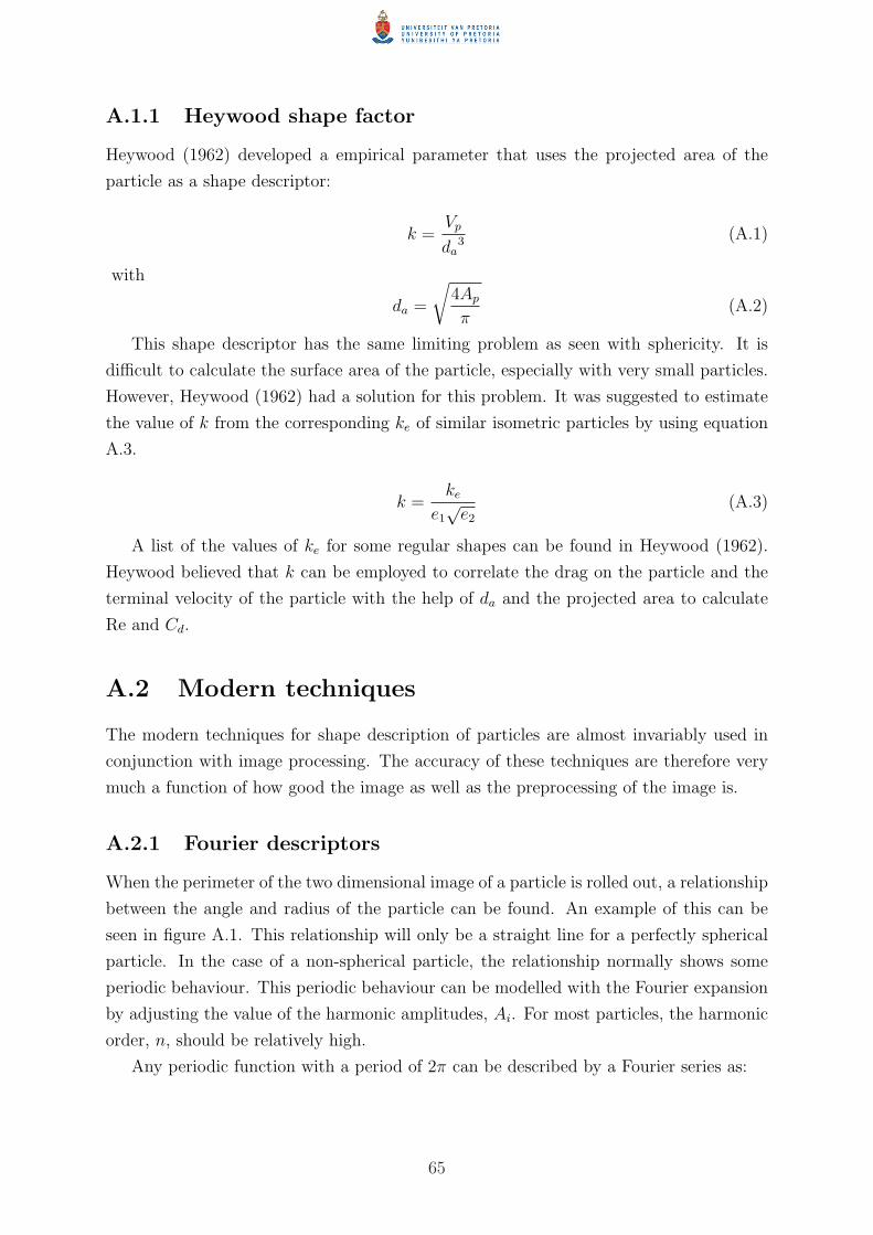
A.1.1 Heywood shape factor
Heywood (1962) developed a empirical parameter that uses the projected area of the
particle as a shape descriptor:
k =Vp
da3 (A.1)
with
da =
√4Ap
π(A.2)
This shape descriptor has the same limiting problem as seen with sphericity. It is
difficult to calculate the surface area of the particle, especially with very small particles.
However, Heywood (1962) had a solution for this problem. It was suggested to estimate
the value of k from the corresponding ke of similar isometric particles by using equation
A.3.
k =ke
e1√
e2
(A.3)
A list of the values of ke for some regular shapes can be found in Heywood (1962).
Heywood believed that k can be employed to correlate the drag on the particle and the
terminal velocity of the particle with the help of da and the projected area to calculate
Re and Cd.
A.2 Modern techniques
The modern techniques for shape description of particles are almost invariably used in
conjunction with image processing. The accuracy of these techniques are therefore very
much a function of how good the image as well as the preprocessing of the image is.
A.2.1 Fourier descriptors
When the perimeter of the two dimensional image of a particle is rolled out, a relationship
between the angle and radius of the particle can be found. An example of this can be
seen in figure A.1. This relationship will only be a straight line for a perfectly spherical
particle. In the case of a non-spherical particle, the relationship normally shows some
periodic behaviour. This periodic behaviour can be modelled with the Fourier expansion
by adjusting the value of the harmonic amplitudes, Ai. For most particles, the harmonic
order, n, should be relatively high.
Any periodic function with a period of 2π can be described by a Fourier series as:
65

5
10
15
20
25
30
210
60
240
90
270
120
300
150
330
180 0
(a) Particle with high sphericity
−5 −4 −3 −2 −1 0 1 20
2
4
6
8
10
12
14
16
18
20
Angle from starting point (Radians)
Par
ticle
rad
ius
(µm
)
(b) Rolled out perimeter of particle with highsphericity
5
10
15
30
210
60
240
90
270
120
300
150
330
180 0
(c) Particle with lower sphericity
−5 −4 −3 −2 −1 0 1 20
5
10
15
Angle from starting point (Radians
Par
ticle
rad
ius
(µm
)
(d) Rolled out perimeter of particle with lowersphericity
Figure A.1: Example of how the particle shape can affect the periodicity of the rolled outparticle perimeter
66

f(θ) = a0 +N∑
n=1
[an cos (nθ) + bn sin (nθ)] (A.4)
This Fourier series is used more commonly in shape description as:
f(θ) = A0 +N∑
n=1
[An cos (nθ + φn)] (A.5)
Fourier descriptors are good enough to describe particles that are close to spherical,
but as soon as the particle show re-entrant behaviour, the ability of the Fourier descriptors
to describe the particle shape breaks down (Clark, 1987). Re-entrant behaviour can be
classified as the event where one angle value has more than one radius value associated
with it. This problem can be circumvented by using the method developed by Zahn &
Roskies (1972). This method have been reported to handle re-entrant shapes very well
(Fong et al., 1979). The Zahn & Roskies method uses a specified length to walk around
the particle. The change in angle as a function of the length walked is then plotted.
The problem with Fourier descriptors is that as already stated, a fairly large amount of
coefficients are required to describe complex particle shapes. The comparison of these
coefficients can become very convoluted.
A.2.2 Fractal dimension
The idea of a fractal dimension was first used by Mandelbrot (1977) where the problem
of the length of the coast of Britain was discussed. The problem exists where the size of
the features taken into account affects the measured length of the coast. In other words,
if the coast is measure in increments of 1 km, small bays and capes will not be ‘seen’,
while if increments of 10 m is used, even large boulders will be ‘seen’. An example of this
is illustrated in figure A.2. With smaller features taken into account the length of the
coast will increase. This means that when atoms is taken into account, the length of the
coast is effectively infinite. The relationship between the features taken into account, or
step length (SL), and the measured length (ML) can be described as:
ML ∝ SLS (A.6)
The fractal dimension have been defined as:
Df = 1− S (A.7)
The fractal dimension is a measure of the ability of a line to fill the space in which it
exists. As the fractal dimension increase, the line has more kinks and micro structures.
The fractal dimension for a 1-dimensional line in a 2-dimensional surface is limited to a
67

−60 −50 −40 −30 −20 −10 0 10−80
−60
−40
−20
0
20
40
60
Actual feature edgeFigure edge as described by steps
(a) Arbitrary figure edge measured with a smallmeasurement length
−60 −50 −40 −30 −20 −10 0 10−80
−60
−40
−20
0
20
40
60
Actual figure edgeFigure edge as described by steps
(b) Arbitrary figure edge measured with a largemeasurement length
Figure A.2: Example of how the measurement length can affect the perimeter length of anarbitrary figure edge
value of between 1 and 2. A straight line has a fractal dimension of 1, while Brownian
motion (Completely random movement) has a fractal dimension of 2. The fractal dimen-
sion for a highly irregular particle should have a value of approximately 1.4 (Flemmer
et al., 1993).
The fractal dimension of a particle can be measured by ‘walking’ around the particle
perimeter with a specified step length and measuring the subsequent perimeter length.
The step length is then decreased and the ‘walk’ is repeated again. The procedure is
repeated up to the smallest step length experimentally measurable. The results of this
procedure is then plotted on a log-log graph where the perimeter length is plotted as a
function of the step length. The fractal dimension can be obtained directly from this
relationship.
The application of the different step sizes to measure the fractal dimension can be seen
in figure A.3. This example gives an good indication that for small step sizes the particle
perimeter is tracked relatively good, with most features included. At a much larger step
size, only the general shape of the particle is tracked. Small features are completely
ignored. As stated already the fractal dimension can be calculated directly from a log-log
plot of the perimeter length as a function of the step length. An example of such a plot
can be seen in figure A.4. The straight line relationship between the perimeter length
and the step length around the particle can clearly be observed on the log-log plot. The
specific particle investigated in figure A.4 has a fractal dimension of 1.012, which is an
indication of a relatively smooth particle with little or no protrusions and indentations.
A.2.3 Polygonal harmonics
The human eye is very good at distinguishing different shapes. It is easy for us to say
where a particle appears to be square, triangular or some other known shape, even though
68

20
40
60
80
30
210
60
240
90
270
120
300
150
330
180 0
(a) Step length of 2.16 µm
20
40
60
80
30
210
60
240
90
270
120
300
150
330
180 0
(b) Step length of 34.5 µm
Figure A.3: An illustration of how the step size around the particle affects the perimeterlength
100
101.806
101.808
101.81
101.812
101.814
101.816
Step length (µm)
Per
imet
er le
ngth
(µm
)
Figure A.4: A log-log plot used to calculate the fractal dimension
69

the particle is not exactly that shape. In theory it should be relatively hard to develop
a technique for an automated system, such as a computer, as computers are very exact.
This would force the technique to have a very long list of rules that do not interfere with
each other, which can be computationally intensive. One technique that gives a proper
indication of the macro shape of a particle is to calculate the polygonal or fractal harmonic
of a particle (Clark, 1987). The basis of polygonal harmonics are exactly the same as that
of fractal dimensions. A specified step size is used to walk around a particle perimeter,
however the process is not terminated once the perimeter has been circumvented but
continues for a specified amount of circumventions. In almost all the cases the path
walked will soon be repeated so that the walk will ‘follow in its own footsteps’. This
repeated walk or harmonic will form a regular polygon, where the steps taken will fall
along the edges of the polygon. With different step lengths used, different polygons will
be found. Normally the large step sizes are started with, therefore the first harmonic
found will be the second harmonic, where two points on opposite sides of the particle
edge are stepped between. The third harmonic will form a triangle inside the particle
perimeter and the fourth harmonic a rhombus. This process can continue as far as the
resolution of the particle edge allows for, but since polygonal harmonics are mostly used
as a macro shape descriptor (Clark, 1987), the highest harmonic of real interest should
be the fifth or sixth harmonic. An example of these harmonics can be seen in figure
A.5. A specific harmonic for an object can exist, and usually do, for more than one step
(a) Simple third harmonic for a particle (b) Simple fourth harmonic for a particle
Figure A.5: Illustration of third and fourth harmonics for a particle
length. The range of step lengths for which a certain harmonic can be found is called the
persistence of that harmonic and can be defined as shown in equation A.8.
Pn =SLnmax
SLnmin(A.8)
70

It has been found that the persistence of the third harmonic is high for triangular par-
ticles, while the persistence of the fourth harmonic is low for triangular particles (Clark,
1987). A list of harmonic persistences found for isometric can be seen in table A.1.
Flemmer et al. (1993) found the third harmonic, P3, to be a good shape descriptor to
Table A.1: Harmonic characteristics for isometric shapes (From Clark (1987))
Shape Persistence of harmonic2nd 3rd 4th
Perfect smooth circle 1 1 1
Equilateral triangle 1 2 1
Square 1.36 1 1.41
Scalene triangle ∼1.5 ∼1.6 1
distinguish between different shapes in correlating fluidised bed hydrodynamics. Clark
et al. (1989) used the second harmonic, P2, to find a correlation between the drag co-
efficient and particle shape. It would therefore seem that there is no ‘golden’ harmonic
to use for shape description, but one has to be found specific for a system. Polygonal
harmonics are however very powerful to describe macro particle shapes.
A.2.4 Piper’s angle and Delta analysis
Cutbill (1971: p.97) as quoted by Flemmer et al. (1993) and Pickett et al. (1991) devel-
oped a technique to take a measure of the surface roughness of a particle. An illustration
of how this technique works can be seen in figure A.6. This technique use an approxi-
mation of the particle silhouette with lines of equal length. These lines can be classified
as leading and following vectors. The angle between the extension of the leading vector
and the following vector can be measured for all of these lines. Note that a following
vector become a leading vector if the next angle needs to be measured. A Piper’s angle
of 0◦ would therefore indicate a straight line. Note that the way Piper’s angle is defined,
the Piper’s angle will always lie between 0◦ and 180◦. A frequency plot of the angles
between the lines are used to indicate the surface roughness of the particle. As a result
of the constant step size used approximate the particle silhouette, the size of the steps
will influence the features taken into account. Pickett et al. (1991) developed a new way
to present the Piper’s angles by plotting the average angle as a function of the step size.
This method of representation allows one to see at which scale the particle is the most
rugged and how rugged the particle is at this scale. A problem associated with Piper’s
71

Leading vector
Following vector
Piper angle
Particle edge
Figure A.6: Illustration of how Piper’s angles are measured
angle is that two different features with a similar Piper’s angle can have completely dif-
ferent hydrodynamic consequences. An example of this can be seen in figure A.7. In
Angle 2
Angle 1
Figure A.7: An illustration of how Piper’s angle can be lacking as a shape descriptor
this example, the protruding feature marked by angle 2 and the receding feature marked
by angle 1 have more or less the same Piper’s angle, but these features will result in
completely different hydrodynamic behaviour for a particle. A modification that can be
used to correct for this short coming in the Piper’s angle is to use the angle between the
lines, either on the inside of the particle or on the outside of the particle. The inside of
the particle refers to the angle between the lines closest to the centroid of the particle,
where outside of the particle refers to the angle furthest from the centroid. When this
modification is used, the Piper’s angle will not lie between 0◦ and 180◦, but between 0◦
and 360◦.
72

A.2.5 Multi-scale roughness descriptor
All of the previously noted techniques either focus on the macro shape (Sphericity, Cir-
cularity and Polygonal harmonics), or micro structure (Heywood shape factor, Fourier
coefficients, Fractal dimension and Piper’s angles) of the particle under investigation. The
problem associated with these techniques are that at least two descriptors are necessary
to properly describe a particle shape. Drolon et al. (2000) developed a technique called
the multi-scale roughness descriptor which is very useful for particle shape description.
This technique utilise the harmonic wavelet transform (HWT) to classify the particle. By
using the HWT as a classifier, it is possible to form a concept on all scales of what the
particle looks like. The wavelet coefficients are calculated at different levels and these
coefficients can then give an indication of the roughness at each of these levels. The lower
levels give an indication of the macro shape of the particle, for example how elongated
it is. Whereas the lower coefficients give an indication of how rough the surface of the
particle is. The mathematics involved in the calculation of the multi-scale roughness
descriptors are rather complex, and since this method will not be used in this study, the
method will not be described in detail here. However, if interested, refer to Newland
(1993) and Drolon et al. (2000) and Drolon et al. (2003).
73

APPENDIX B
Particle data extraction and manipulation
To process the shape information of the particles, the particle’s shape will have to be
available in a data set that can be processed mathematically. The simplest way to do
this is to have the particle’s perimeter represented as a data set of the distance from the
centroid of the particle, r, and the swept angle from the starting position, θ. The starting
position can be chosen arbitrarily. This data set will henceforth be referred to as the r-θ
data. In figure B.1(a) an illustration can be seen of what is meant by r and θ.
rθ
(a) Full colour image of the particles obtainedfrom the microscope with r and θ indicated
(b) Example of grayscale image after manipula-tion of the full colour image
Figure B.1: Manipulation of image obtained from microscope from full colour image (a) to agreyscale image (b)
Note that both the light microscope and the SEM produces JPEG images. The process
to extract the data from an image of either sources is therefore the same.
74

B.1 Image manipulation
JPEG images are full colour, high resolution photos, as can be seen in figure B.1(a). To
be able to obtain the r-θ data with Matlab, a black and white image is required. The
black and white image can be obtained by thresholding a grayscale image, which in turn
is found by processing the full colour image. These steps have to be done for each image
taken of the particles.
B.1.1 Grayscale image
The grayscale image is a matrix where each cell in the matrix has a value of between
0 and 255, where 0 represents black and 255 represents white. The difference between
the grayscale and the full colour image is that the full colour image has 3 matrices
superimposed on each other. These matrices contain the intensity of the red, blue and
green channels in the cells, with 0 being none of the specific colour and 255 being the full
intensity of the specific colour.
To find a grayscale image that contains the most available information about the
particles, the colour channel has to be chosen with the highest amount of sharp contours
in intensity. This can mathematically be seen as the channel with the highest sum of
derivatives.
The resultant grayscale image obtained from figure B.1(a) after choosing the best
channel can be seen in figure B.1(b).
B.1.2 Black and White Image
The greyscale image in figure B.1(b) has two main features. These features are the
background and the particles. Because of dirt on the microscope lens, rough features,
etc, it is expected that noise will be present in both these features. This means that
a Gaussian distribution of intensity can be expected for each feature. This bimodal
Gaussian distribution can be seen in figure B.2. With this information known, the best
value to threshold the grayscale image at, is the intensity level at which the two Gaussian
distributions intersect.
With the threshold value for the image known, the black and white image can be
displayed. Therefore all the cells in the matrix of the greyscale image with a intensity
value below the threshold value will be displayed. This can be seen in figure B.3(a).
However this figure still shows some noise and holes within the particles. Since it is
known that all the particles are solid, these holes can be filled and the noise in the image
can be cleaned. The resultant, cleaner image can be seen in figure B.3(b). The edge
of the particle in a black and white image can be used to calculate the radius of the
particle all along the edge, as well as the angle between the radius line and the radius
75

40 60 80 100 120 140 160 180 200 220 2400
2
4
6
8
10
12
14
16
18x 10
4
Intensity Value
Figure B.2: Bimodal Gaussian distribution for the range of intensities in figure B.1(b)
(a) Black and white image obtained after thresh-olding the grayscale image in figure B.1(b)
(b) Cleaned black and white image ready for par-ticle shape extraction
Figure B.3: Noisy black and white image (a) obtained after thresholding and cleaned blackand white image (b)
76

line of the starting position. A plot of one of the particles, in terms of the radius and the
angle can be seen in figure B.4. This is the required r-θ data from which further shape
characterisation is possible.
20
40
60
80
30
210
60
240
90
270
120
300
150
330
180 0
Figure B.4: Extracted particle border of one of the particles in figure B.3. Note that thedimension of the radius is µm
B.2 Particle shape characterisation
With the 2-dimensional data available for each of the particles, processing of the data can
be done to characterise the shapes with the 2-dimensional shape characterisation methods
discussed in appendix A. The sphericity of the particle cannot be properly calculated with
2-dimensional methods. However, the circularity can be calculated with ease by using
equation 2.17 and can be used in the same way that the sphericity of a particle is used.
For all the modern shape classification techniques, it is necessary to approximate the
particle edge with an array of lines that has the same length. The algorithm that approx-
imates the edge starts off at a specified data point. The distance between the starting
point and the next data point are then measured using the cosine rule in trigonometry.
The distance is then compared with the specified step length (The length that each of the
lines in the array of lines approximating the particle edge should have). If the distance
between the data points are less than the specified step length, the distance between
the starting point and the next data point is calculated. This process is continued until
either the distance is exactly equal to the specified step length, or the distance exceeds
the specified step length. In the case where the distance is equal to the specified step
77

- Centroid- Pixels representing particle perimeter- Additional inserted perimeter pixels- Steps depicting perimeter- Radius lines to perimeter pixels
Figure B.5: A schematic illustration of how the particle perimeter is approximated with aseries of lines of equal length
length, the data point to which this distance was measured is made the starting point
and the process is repeated. However, if the distance exceeds the specified step length,
a new data point is created by means of interpolation to which the distance is exactly
the specified step length. This newly created data point is then made the starting point
and the process is repeated. A schematic that shows this process graphically can be seen
in figure B.5. This stepping around the particle perimeter is repeated until the particle
perimeter is circumvented fully. The last line in the array are sometimes not of the same
length as the other steps in the array, however, this is not a problem as the contribution
of the last step to the total result is insignificant.
78

APPENDIX C
Particle shape analysis results
C.1 Modern techniques
C.1.1 Fractal dimension
The fractal dimension should, as stated in section A.2.2 give an indication on how rugged
the surface of the particles are. To be able to use the fractal dimension to calculate the
surface roughness of a particle, care have to be taken to ensure that the perimeter of
the particle is in a sufficiently good enough resolution. The fractal dimensions for the
mixtures can be seen in figure C.1. The results obtained in this figure is the opposite
of what can be expected after looking at figure 3.5. It is expected that the fractal
dimension of the milled FeSi should be much higher than that of the atomised FeSi.
The explanation for this lack of compatibility with what one would expect is that the
resolution of the images are simply just not high enough. To be able to quantify the
roughness of a particle surface, the perimeter of one particle should fill the entire image.
However, the time required to take a sufficient amount of images of individual particles on
the SEM so that a statistically meaningful average is obtained is impractical. A further
problem associated with the fractal dimension is that small artifacts on the perimeter of
the particle can severely affect the calculated fractal dimension.
C.1.2 Piper’s angle
Piper’s angle is another technique that measures the surface roughness of a particle with
the aid of image processing as described in section A.2.4. The Piper’s angles are a
function of the step size of the approximation of the particle edge. The same technique
was used as described by Pickett et al. (1991), but instead of using the average Piper’s
angle for the batch of particles, the standard deviation of the Piper’s angles for the batch
79

Figure C.1: The fractal dimensions for both the atomised and milled FeSi expressed in afrequency plot. Dfavg for milled FeSi = 1.056 and Dfavg for atomised FeSi = 1.065
of particles was used. The optimum step size was found to be 0.1×deq of the particles.
The frequency plot for the atomised and milled FeSi can be seen in figure C.2. As with
the fractal dimension, the Piper’s angle has severe inadequacies when trying differentiate
between the atomised and milled FeSi. This is as a result of the resolution in the images of
the particles. If a higher detail image can be taken of the particles, these techniques which
measure particle shape based on micro structure of the particles can be used, however,
with the available photos, the only techniques that should work properly to differentiate
between the particles are those that measure macro shape.
C.1.3 Polygonal harmonics
Since all the shape description techniques which are based on the classification of the
micro structure of the particle perimeter seems to be inefficient in differentiating between
the two solid types, further investigation in shape description techniques which are based
on the macro shape of the particle should be done. The persistence of polygonal harmonics
has a good reputation for differentiating between different particle shapes. The results of
the polygonal harmonics can be seen in figures C.3, C.4, C.5 and C.6.
The higher persistence of the second polygonal harmonic in the atomised particles
is an indication that these particles are more elongated than the milled particles. This
is in agreement with the process in which the atomised particles are made. The milled
particles tend to be in their most stable position, which orientates the breadth and width
80
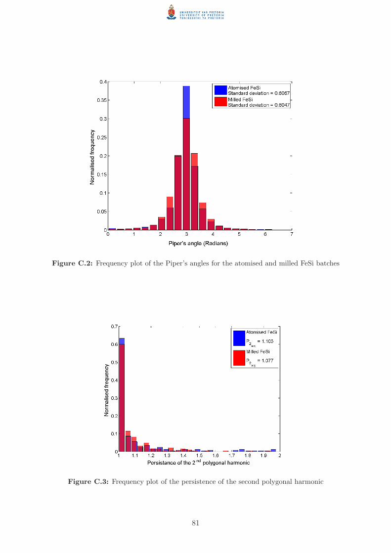
Figure C.2: Frequency plot of the Piper’s angles for the atomised and milled FeSi batches
Figure C.3: Frequency plot of the persistence of the second polygonal harmonic
81

Figure C.4: Frequency plot of the persistence of the third polygonal harmonic
Figure C.5: Frequency plot of the persistence of the fourth polygonal harmonic
82

Figure C.6: Frequency plot of the persistence of the fifth polygonal harmonic
of the particles perpendicular to the direction of the electron beam from the SEM. This
would explain why the milled particles have a low persistence for the second polygonal
harmonic.
The third harmonic clearly indicates that the atomised particles have a mostly square
shape, which would explain why persistence of the third harmonic is so low. The milled
particles have a much wider distribution in the persistence of the polygonal harmonics,
which indicates that a fair amount of triangularly shaped particles exists in the batch of
particles.
The fourth harmonic confirms the square nature of the atomised particles, as seen with
the third harmonic. This can also be explained by the method in which the atomised
particles are produced, where the particles that do not separate into proper droplets form
elongated globules so that they have rectangular shapes. The persistence for the milled
particles are slightly higher, however, it is much lower than one would expect. With the
plethora of irregular shapes found in the milled particles, it can only be expected that
some are squarish, but the persistence of the fourth harmonic is much lower than that of
the third harmonic. This means that the predominant shape among the milled particles
are the slightly triangular ones.
The higher persistence in the fifth harmonic for the atomised particles can also be
confirmed by the technique in which the atomised particles are formed. Even though the
particles are mostly spherical in nature, quite a few of them get slightly elongated in the
formation process.
The polygonal harmonics gives a good qualitative idea of how the morphology of the
batches of particles differ, however, because such a large fraction of the particles have a
83

persistence of 1 for most of the harmonics, it is not possible to get a quantitative idea of
the particle shapes.
84