The Effect of Foreign Aid on Income Inequality: Evidence from Panel Cointegration

by Dierk Herzer Peter Nunnenkamp

No. 1762 | March 2012

Kiel Institute for the World Economy, Hindenburgufer 66, 24105 Kiel, Germany

Kiel Working Paper No. 1762 | March 2012

The Effect of Foreign Aid on Income Inequality: Evidence from Panel Cointegration

Dierk Herzer and Peter Nunnenkamp

Abstract: This paper examines the long-run effect of foreign aid on income inequality for 21 recipient countries using panel cointegration techniques to control for omitted variable and endogeneity bias. We find that aid exerts an inequality increasing effect on income distribution.

Keywords: Inequality, foreign aid, panel data, cointegration.

JEL classification: D31, F35, C23 Dierck Herzer Helmut-Schmidt-University Hamburg Holstenhofweg 85 D-22043 Hamburg, Germany phone: +49-40-6541-2775 Fax: +49-40-6541-2118 E-mail: herzer@hsu-hh.de

Peter Nunnenkamp Kiel Institute for the World Economy Hindenburgufer 66 D-24105 Kiel, Germany phone: +49-431-8814-209 Fax: +49-431-8814-500 E-mail: peter.nunnenkamp@ifw-kiel.de

____________________________________ The responsibility for the contents of the working papers rests with the author, not the Institute. Since working papers are of a preliminary nature, it may be useful to contact the author of a particular working paper about results or caveats before referring to, or quoting, a paper. Any comments on working papers should be sent directly to the author. Coverphoto: uni_com on photocase.com

1. Introduction

Taking donor strategies at face value, the urgent need for foreign aid of poor and

disadvantaged people living in developing countries represents the overarching motive of official

development assistance (ODA). The donor community committed itself in 2000 to achieving the

Millennium Development Goals which would mainly benefit the poorest population segments and,

thereby, reduce inequality in the recipient countries. Apart from halving absolute poverty by 2015,

particularly relevant targets include the provision of universal primary education and universal

access to reproductive health. Donors also agreed at the G8 summit in Gleneagles in 2005 that ODA

has to be scaled up substantially to finance these important dimensions of pro-poor growth.

According to Sachs and McArthur (2005: 347), ODA is a critical constraint to finance “what is

crushingly expensive for the poorest of the poor.” Increases in ODA, if properly directed, could thus

improve the poverty reducing impact of a given rate of economic growth. Pro-poor growth, in turn,

could enhance political stability and social cohesion which tend to be undermined by increasing

inequality (OECD, 2006).1

It is open to debate, however, whether ODA effectively supports pro-poor growth. Recent

surveys on the growth impact of aid come to sharply opposing verdicts. Doucouliagos and Paldam

(2009: 433) conclude that “after 40 years of development aid, the preponderance of the evidence

indicates that aid has not been effective.” By contrast, McGillivray et al. (2006: 1031) summarize

that more recent research “agrees with its general finding that aid works to the extent that in its

absence, growth would be lower.” Yet, even this positive assessment does not resolve the question

of whether it is primarily the poor whose income prospects improve through ODA.2 Anecdotal

evidence rather suggests that mainly the political elite benefits from aid. It is estimated that the

former president of Zaire, Mobutu Sese Seko, looted the treasury of at least $5 billion (an amount 1 Bourguignon et al. (2009: 9) argue that if the high level of global income inequality “were to exist within a single country, that country would probably experience substantial social strive.” 2 On the other hand, the negative verdict of Doucouliagos and Paldam (2009) does not necessarily preclude favorable effects on the distribution of income as aid may alleviate poverty without having discernible average growth effects (Arvin and Barillas, 2002; Chong et al., 2009).

1

equal to the country’s entire external debt at the time he was ousted in 1997). The funds allegedly

embezzled by the former presidents of Indonesia and the Philippines, Mohamed Suharto and

Ferdinand Marcos, are still higher (Svensson, 2005).

In contrast to the fairly large literature on growth effects, the distributional effects of ODA

have received scant attention in previous empirical research. It is important to fill this gap in order

to improve the allocation of aid and its effectiveness. Theoretical considerations show that aid may

induce self-interested recipients to engage in rent-seeking activities aimed at appropriating resource

windfalls (Svensson, 2000; Hodler, 2007; Economides et al., 2008). Moreover, donors may allocate

aid in a way that deviates from the pro-poor growth rhetoric. As discussed in more detail in Section

2, several channels exist through which aid may result in more pronounced income inequality. The

few existing empirical findings are mixed. Chong et al. (2009), using cross-section and system

GMM panel techniques, find that aid has no robust effect on inequality. The random effects panel

analysis by Bjørnskov (2010) reveals that the interaction of foreign aid and democracy in the

recipient country is robustly and positively associated with income inequality. Shafiullah (2011)

estimates fixed and random effects models and concludes that aid reduces income inequality.3

Against the backdrop of scarce and ambiguous findings, we re-assess the question of the

distributional effects of foreign aid. Specifically, we contribute to the empirical literature by

employing panel cointegration techniques to examine the long-run effect of aid on income

inequality. Panel cointegration estimators are most appropriate in the present context. We argue in

Section 3 that they are robust under cointegration to a variety of estimation problems that often

plague empirical work, including omitted variables, slope heterogeneity, and endogenous

regressors. To anticipate the results, we find that aid exerts an inequality increasing effect on the

distribution of income.

3 Bourguignon et al. (2009: 1) find that aid has a weak equality enhancing effect on the international distribution of income. But these authors abstract from “the admittedly critical element of within country inequality.”

2

The remainder of this paper is composed of four sections. In Section 2, we discuss the

related literature. Section 3 sets out the basic empirical model and describes the empirical

methodology. The data and the estimation results are presented in Section 4, and Section 5

concludes.

2. Related literature

Two critical conditions would have to be met for ODA to be effective in reducing income

inequality in recipient countries.4 Donors would have to allocate aid in line with their rhetoric on

pro-poor growth, by targeting the most needy and deserving. At the same time, the authorities in the

recipient countries would have to ensure that aid actually reaches the poor. The following

arguments suggest that both conditions tend to be violated once it is taken into account that foreign

donors are not purely altruistic and local authorities have incentives to divert aid funds for personal

benefit.

From the literature on aid allocation across recipient countries it is well known that donors

have both altruistic and egoistic motives (e.g., Berthélemy, 2006). Specifically, this literature

reveals that ODA is partly motivated by commercial and political self-interest. According to

Alesina and Dollar (2000: 33), there is “considerable evidence that the direction of foreign aid is

dictated as much by political and strategic considerations, as by the economic needs and policy

performance of the recipients.”5 Alesina and Weder (2002) find that ODA is distributed

indiscriminately between countries with honest and corrupt governments. Admittedly, the cross-

country evidence does not allow any direct inference as to the distributional effects of ODA within

recipient countries. Little is known about the distribution of aid within countries, either

geographically or between segments of the population. Yet selfish donor motives are likely to

4 For a similar line of reasoning, see Drazen (2007: 669), according to whom the ineffectiveness of aid may be “due to the actions of aid agencies (e.g., giving aid repeatedly, no matter what performance has been) and/ or recipients (e.g., misuse of aid).” 5 More recently, Fleck and Kilby (2010) find that the emphasis placed on need has weakened for core recipients of US aid during the War on Terror.

3

compromise the needs- and merit-based allocation of aid within countries, too. For instance,

commercial donor interests may have as a consequence that ODA, e.g., in the area of physical

infrastructure, is concentrated in industrial clusters rather than remote areas where the poorest

people are living. Likewise, using aid as a means to buy political support by the local elite implies

that it favors the rich rather than the poor within a particular country.6

Even if donor countries did not use aid to foster commercial or political self-interest, the

incentives of aid agencies might work against inequality reducing effects of ODA. As noted by

Drazen (2007), agencies have strong incentives to continue disbursing aid independent of whether it

is effective. The incentive to “push money out the door” (Drazen, 2007: 672) also implies that

agencies favor large-scale operations rather than small projects reflecting indigenous creativity

(Easterly, 2006), even though the latter may be better suited to reduce inequality. Information

asymmetries create additional incentive problems working against inequality reducing effects of

aid. On the one hand, taxpayers in the donor countries usually do not have the information required

to assess the success or failure of specific aid interventions. On the other hand, political authorities

are interested in proving the case for ODA. As a result, aid agencies might be inclined to ‘plant their

flag’ and engage in highly visible projects in order to secure future funding. This may explain why

Thiele et al. (2007) find that various donors prefer granting aid for higher levels of education, but

spend very little on primary education even though the MDGs require donors to concentrate on

universal access to basic education as a pre-condition for pro-poor growth. Moreover, agencies that

have to demonstrate success to political authorities can be expected to minimize the risk of project

failure which weakens their incentive to operate in remote regions where aid may be needed most.7

In other words, the poverty orientation of aid agencies could be affected by pressure from their

6 In a similar vein, Shafiullah (2011: 91) argues that aid tends to strengthen the political, social and economic influence of local elites that serve the donors’ political and commercial interests. 7 This line of reasoning is closely related to the principal-agent model of Fruttero and Gauri (2005). These authors argue that financial dependence of NGOs (the agents) on external funding (notably from official principals) drives a wedge between organizational imperatives related to future funding and charitable objectives in locations where NGOs are active.

4

principals to demonstrate project-related impact in the short run. Immediate and visible results are

easier to achieve when addressing less entrenched forms of poverty. However, inequality reducing

effects of ODA become less likely if agencies are reluctant to work in ‘difficult environments.’

Furthermore, aid recipients are typically subjected to conditionality through which donors

may affect the effectiveness of aid (Dalgaard, 2008). Specifically, aid in the past often took the

form of structural adjustment lending which required the recipients to undertake policy reforms that

donors deemed necessary for aid to be effective. However, critics of conditional aid blamed

structural adjustment programs for having negative distributional effects, e.g., by involving cuts in

local government spending on poverty relevant items such as basic education and health.8 Negative

distributional effects may also result from aid-related Dutch disease. Aid inflows may impair a

country’s competitiveness through real exchange rate appreciation (Doucouliagos and Paldam,

2008; Rajan and Subramanian, 2011). Poorer population segments may be affected most seriously,

either because real incomes earned in the informal sector are not protected against higher inflation

or because of lay-offs in low-skilled labor intensive production for exports (Bjørnskov, 2010).

Turning to the authorities in the recipient countries, it is widely acknowledged in the

literature that local incentive problems stand in the way of ODA reaching the poor.9 Svensson’s

(2000) seminal contribution departs from the puzzle that the macroeconomic effects of ODA are

ambiguous even though it represents an important source of revenue in various recipient countries.

Svensson explains this puzzle by developing a game theoretic rent-seeking model in which social

groups within the recipient country compete over common-pool resources. Foreign aid may be used

to provide public goods, or it may be appropriated for private benefit. The latter may happen “either

by means of direct appropriation (e.g., seizure of power) or manipulation of bureaucrats and

politicians to implement favorable transfers, regulations or other redistributive policies” (Svensson,

8 See Easterly (2003) for a critical discussion. 9 See Drazen (2000, section 12.9) for an overview.

5

2000: 438). From the model, it can be derived theoretically that an increase in aid may even reduce

the supply of public goods. It follows that aid does not necessarily lead to increased welfare.

The effects of aid on rent seeking and corruption in the recipient countries figure

prominently in more recent papers, too. However the focus is typically on adverse growth

implications (e.g., Hodler, 2007; Economides et al., 2008; Angeles and Neanidis, 2009).10 In the

present context, it is important to note that local elites and rich population segments tend to get the

upper hand in aid-induced rent-seeking contests. Almost by definition, local elites are endowed with

a disproportionate share of the country’s economic and political power (Angeles and Neanidis,

2009). At the same time, the transfer that a group receives tends to be proportional to its

expenditures on rent seeking as a fraction of total expenditures on rent seeking by all groups

(Drazen, 2000: 606). Taken together, aid-induced rent seeking tends to favor the rich.11 For

instance, aid may exacerbate inequality by aggravating unequal access to education (Shafiullah,

2011). Indeed, Reinikka and Svensson (2004) find that the extent to which school grants in Uganda

actually reached the ultimate beneficiaries depends on the bargaining power of local communities.

Schools in better-off communities received a higher share of their entitlements.

In sum, there are various channels – involving agents on the side of both donors and

recipients – through which aid may affect the distribution of income within aid-dependent countries.

Importantly, the subsequent panel cointegration analysis does not attempt to isolate the effects of

ODA on income distribution working through specific transmission channels. To the contrary, our

objective is to capture overall effects; this provides a major argument in favor of the bivariate

approach and against controlling for factors such as exchange rates and local institutions through

10 As mentioned in the Introduction, few empirical studies focus on the distribution of income within recipient countries, notably Chong et al. (2009), Bjørnskov (2010), and Shafiullah (2011). Boone (1996: 293) uses infant mortality as the dependent variable which “can be considered a flash indicator of improvements in economic conditions of the poor.” 11 Boone (1996) raises the hypothesis that democratic and liberal political regimes use aid differently from ‘elitist’ regimes. However, Boone’s empirical findings reveal that all political regimes direct aid to wealthy elites.

6

which aid may affect the distribution of income. Thereby, we also avoid serious measurement

problems, e.g., with respect to rent-seeking activity (Economides et al., 2008).

3. Model and empirical methodology

The analysis will examine the long-run relationship between foreign aid and income

inequality. In this section, we present the basic empirical model, discuss some econometric issues,

and describe the empirical methodology.

3.1. Model

Following common practice in (panel) cointegration studies (see, e.g., Herzer, 2008;

Pedroni, 2007; Chintrakarn, et al., 2012), we estimate a bivariate model of the form

ititiit AidaInequality εβ ++= , (1)

where Inequalityit stands for the estimated household income inequality (EHII) in Gini format

(measured on a 0 to 100 scale) of country i in year t and Aidit represents net aid transfers (NAT) to i

in t (as a percentage of GDP). The coefficient β in Eq. (1) can be interpreted as the long-run

elasticity of inequality with respect to aid, measuring the change in the EHII Gini index in response

to a one percentage point change in the share of aid in GDP. Moreover, we include country-specific

fixed effects, , to control for any country-specific omitted factors that are relatively stable over

time.

ia

Eq. (1) assumes that there is a long-run bivariate relationship between aid and inequality and

that therefore no other variables are required to produce unbiased estimates of the long-run effect of

aid on inequality. An attractive feature of Eq. (1), and the reason why we use it, is thus its

parsimonious structure. However, a necessary condition for Eq. (1) to be a correct description of the

data is that both the individual time series for the EHII Gini coefficient and the individual time

series for aid (relative to GDP) are nonstationary or, more specifically, integrated of the same order

and that Inequalityit and Aidit form a cointegrated pair.

7

A regression consisting of two cointegrated variables has a stationary error term, itε , in turn

implying that no relevant integrated variables are omitted; any omitted nonstationary variable that is

part of the cointegrating relationship would enter the error term, thereby producing nonstationary

residuals and thus leading to a failure to detect cointegration. Eq. (1) would in this case represent a

spurious regression in the sense of Granger and Newbold (1974) (if the variables are nonstationary

and not cointegrated). If, on the other hand, a cointegrating relationship exists among a set of

nonstationary variables, the same cointegrating relationship also exists in extended variable space

(Johansen, 2000). Thus, an important implication of finding cointegration is that no relevant

integrated variables are omitted in the cointegrating regression. Cointegration estimators are

therefore robust to the omission of non-stationary variables that do not form part of the

cointegrating relationship (Pedroni, 2007).

Of course, there are several factors (such as economic growth, trade, foreign investment, and

redistribution policies) that affect inequality. Adding further variables may therefore result in

further cointegrating relationships. Since the cointegration property is invariant to extensions of the

information set, the estimates will not be significantly affected by the presence (or absence) of

additional variables (Juselius, 2006). This justifies considering small subsystems, such as Eq. (1) (if

the variables are cointegrated), while the inclusion of additional variables would unnecessarily

increase the number of cointegrating equations that would have to be identified and estimated.

Another assumption underlying Eq. (1) is that income inequality is endogenous in the sense

that, in the long run, changes in aid flows over time cause changes in income distribution over time.

However, although cointegration implies the existence of long-run causality in at least one direction

(Granger, 1988), income distribution may also act as a determinant of aid flows. For example, it

may be that donors reward more equal countries with increased aid for successful poverty reduction

or that aid goes to countries with higher inequality because these countries have higher poverty

8

rates. The empirical implication is that it is important not only to examine the data for unit roots and

cointegration, but also to account for this potential endogeneity.

Another important issue is the potential cross-country heterogeneity in the relationship

between aid and inequality. Countries differ in terms of per capita income, economic, political, and

social structures (and other characteristics). The implicit assumption of traditional, homogeneous

panel estimators that the coefficients on the variables of interest are the same across all countries

can therefore be unduly restrictive. The problem is that homogeneous (within-dimension) estimators

may produce inconsistent and potentially misleading estimates in the presence of slope

heterogeneity (Pesaran and Smith, 1995). For this reason, we use heterogeneous (between-

dimension) panel estimators based on the mean group approach and thus allow the coefficients to

vary across countries.12

A final econometric issue is the potential cross-sectional dependence among the variables

through common time effects. Cross-sectional dependence may be the result of global business

cycles and other common factors. Examples of such common factors that affect aid flows in several

countries at the same time might include global natural disasters, regional wars and famines, and

international donor coordination. Inequality is likely to be affected by common factors such as

technological progress and the globalization of trade and investment. Given that standard panel unit

root and cointegration tests may be biased in the presence of such cross-sectional dependence, we

also use recent advances in panel data econometrics to account for this issue.

3.2. Empirical methodology

As the above discussion implies, the first step in the analysis is to examine the time series

properties of the data. To this end, we use the panel unit root test of Im, Pesaran, and Shin (2003)

(IPS), which is based on the augmented Dickey-Fuller (ADF) regression for the ith cross-section

unit: 12 Group-mean estimators are based on the between dimension of the panel, while the pooled estimators are based on the within dimension of the panel (Pedroni, 2000).

9

it

k

jjitijitiitit

i

xxzx εϕργ +∑ Δ++=Δ=

−−1

1' , (2)

where ki is the lag order and zit represents deterministic terms (such as a constant and a trend). The

unit root null hypothesis, 0:0 =iH ρ , i∀ =1, 2, …, N, is tested against the alternative of (trend)

stationary, 0:1 <iH ρ , i = 1, 2, …, ; 1N 0=iρ , 11 += Ni , 21 +N , …, N, using the standardized t-bar

statistic

[ ]v

tN NTt

μ−=Γ , (3)

where NTt is the average of the N cross-sectional ADF t-statistics, and μ and ν are, respectively, the

mean and variance of the average of the individual t-statistics, tabulated by Im et al. (2003).

However, the standard IPS test can lead to spurious inferences if the errors, εit, are not

independent across i (for example, due to common shocks). Therefore, we also employ the cross-

sectionally augmented IPS test proposed by Pesaran (2007), which is designed to filter out the

cross-section dependence by augmenting the ADF regression with the cross-section averages of

lagged levels and first-differences of the individual series. Accordingly, the cross-sectionally

augmented ADF (CADF) regression is given by

it

k

jjtijti

k

jjitijitiitit vxxxxzx

ii

+Δ++Δ++=Δ ∑∑=

−−=

−−0

11

1' ηαϕργ , (4)

where tx is the cross-section mean of xit, tx = . The cross-sectionally augmented IPS

statistic is the simple average of the individual CADF statistics and is defined as

∑=− N

i itxN1

1

CIPS = t-bar = , (5) ∑=

−iN

iitN

1

1

where is the OLS t-ratio of it iρ in Eq. (4) Critical values are tabulated by Pesaran (2007).

Another potential problem is that standard unit-root tests are biased towards a non-rejection

of the null hypothesis of a unit root in the presence of structural breaks. Therefore, as an additional

10

test, we apply the structural break unit-root test of Perron (1997) to each individual series of the

panel. This test has that advantage that the potential break points are determined endogenously from

the data. We estimate two models:

tt

k

iitttt excxaTBDtbDUx 11

111111111 )( +Δ+++++= −

=− ∑δθμ , (6)

tt

k

iitt

ttt

excxax

xDTtbx

211

212

2222

ˆˆ

ˆ

+Δ+=

+++=

−=

− ∑)

δμ, (7)

where 1μ and 2μ , respectively, are constants, t is a deterministic trend, TB ∈ T (1 ≤ t ≤ T) denotes

the time at which the break in the trend function occurs and DUt = 1(t > TB), D(TB)t =1(t = TB + 1),

DTt = 1(t > TB)(t –TB) are indicator dummy variables for the break at time TB.

Eq. (6) allows for a change in the intercept of the trend function, while Eq. (7) allows for a

change in the slope of the trend function. TB is selected as the value which minimizes the t-statistic

for testing a1 = 1 and a2 = 1, respectively:

),,()( ˆ* kTBitMinit aTBa = , (8)

where is the t-statistic for testing a = 1 under model i = 1, 2 [Eq. (6) and (7)]. If

exceeds (in absolute value) the critical value reported by Perron (1997), the null

hypothesis of a unit root is rejected in favor of (broken) trend stationarity.

),,(ˆ kTBita

),,(ˆ kTBitMin aTB

If, as expected, the variables are nonstationary (because of the presence of a unit root), the

next step is to test for cointegration. We use the standard tests of Pedroni (1999) and Kao (1999) for

this purpose. It is well known, however, that these tests may suffer from severe size distortions in

the presence of cross-sectional dependence.

To also test for cointegration in the presence of possible cross-sectional dependence, we use

a two-step residual-based procedure in the style of Holly et al. (2010). Specifically, we employ the

common correlated effects (CCE) estimation procedure of Pesaran (2006) in the first step. Like the

cross-sectionally augmented IPS test, the CCE estimator allows for cross-sectional dependencies

11

that potentially arise from multiple unobserved common factors and permits the individual

responses to these factors to differ across countries. It augments the cointegrating regression (Eq.

(1)) with the cross-sectional averages of the dependent variable and the observed regressors as

proxies for the unobserved factors. Accordingly, the cross-sectionally augmented cointegrating

regression for the ith cross-section is given by

ittitiitiiit AidgInequalitygAidaInequality ξβ ++++= 21 , (9)

where tInequality and tAid are the cross-section averages of Inequalityit and Aidit in year t. In the

second step, we compute the residuals, itμ̂ , of the individual CCE long-run relations (estimated

using Eq. (9)), , and apply the CADF test to the computed residuals,

including an intercept. This allows us to account for unobserved common factors that could be

correlated with the observed regressors in both steps.

ititiit AidInequality μβ ˆˆ +=

If there is evidence of cointegration between Inequalityit and Aidit, the long-run effect of aid

on income inequality is estimated using the group-mean fully modified ordinary least squares

(FMOLS) and dynamic ordinary least squares (DOLS) estimators suggested by Pedroni (2001).

Pedroni (2000, 2001) emphasizes several advantages of between-dimension group-mean-based

estimators over the within-dimension approach. For example, the between-dimension approach

allows for greater flexibility in the presence of heterogeneous cointegrating vectors, whereas under

the within-dimension approach, the cointegrating vectors are constrained to be the same for each

country (as noted above). Another advantage of the between-dimension estimators is that the point

estimates provide a more useful interpretation in the case of heterogeneous cointegrating vectors,

since they can be interpreted as the mean value of the cointegrating vectors, which does not apply to

the within estimators. And finally, the group-mean estimators suffer from a much lower level of

small-sample-size distortions than is the case with the within-dimension estimators.

In general, group-mean estimators involve estimating separate regressions for each country

and averaging the slope coefficients:

12

. (10) ∑=−=

N

i iN1

1 ˆˆ ββ

The t-statistic is the sum of the individual t-statistics divided by the root of the number of cross-

sectional units:

Ntt N

i i/

1 ˆˆ ∑==

ββ. (11)

The basic idea behind both the FMOLS estimator and the DOLS estimator is to account for

possible serial correlation and endogeneity of the regressor(s). Thus, an important feature of these

estimators is that they generate unbiased estimates for variables that cointegrate, even with

endogenous regressors. Clearly, this is an important advantage for applications such as the present

one since one cannot exclude the possibility that inequality is also a determinant of aid flows (as

discussed above). In addition, the estimators are superconsistent under cointegration, and they are

also robust to the omission of variables that do not form part of the cointegrating relationship.

The FMOLS estimator employs a non-parametric correction to eliminate the endogeneity

bias using εit and ΔAidit, whereas the DOLS estimator employs a parametric correction for the

potential endogeneity by augmenting Eq. (1) with leads, lags, and contemporaneous values of the

differenced aid variable:

it

k

kjjitjitiiit

i

i

AidAidaInequality νβ +∑ ΔΦ++=−=

− . (12)

A potential disadvantage of the DOLS procedure in comparison to the FMOLS method is that the

estimates may be sensitive to the choice of the lead and lag structure.

However, both the FMOLS estimator and the DOLS estimator may be biased in the presence

of cross-sectional dependence. Therefore, we check the robustness of our results by using the CCE

mean group (CCEMG) estimator of Pesaran (2006). This estimator is the simple average of the

individual CCE estimators given by Eq. (9).

13

4. Data and empirical results

4.1. Data

Several studies have used the Gini data set constructed by Deininger and Squire (1996).

However, it is well known at least since the work of Atkinson and Brandolini (2001) that the

Deininger-Squire data suffer from deficiencies such as sparse coverage, problematic measurements,

and the combination of diverse data types into a single dataset, thus limiting the comparability, not

only across countries but also over time. Therefore, many studies rely on Gini data from the

Luxembourg Income Study (LIS) database or the UNU-WIDER World Income Inequality Database

(WIID). The major deficiency of all these sources is the lack of continuous and consistent inequality

data over time (Galbraith, 2009).

In this paper, we use the estimated household income inequality (EHII) data set developed

by the University of Texas Inequality Project (UTIP, 2008). These data are fully comparable across

space and time (Galbraith and Kum, 2005). Another advantage is that the EHII data are available

for a reasonably large number of countries over a sufficiently long and continuous time period.

The EHII index is in Gini format (measured on a 0 to 100 scale) and is constructed by

combining information from the Deininger-Squire data set with information from the UTIP-UNIDO

dataset. The latter is a set of measures of manufacturing wage inequality, using the between-groups

component of a Theil index, measured across industrial categories in the manufacturing sector

based on the Industrial Statistics database of the United Nations Industrial Development

Organization (UNIDO). Specifically, the EHII index is computed by regressing the Deininger-

Squire Gini indices on the UTIP-UNIDO Theil inequality measures (and on several control

variables), and then using the predicted values as (estimated) Gini coefficients. The intention of this

procedure is to separate the useful from the doubtful information in the Deininger-Squire data set

(Galbraith and Kum, 2005).

14

Many of the more recent income inequality studies use the EHII Gini coefficient (Meschi

and Vivarelli, 2009; Gimet and Lagoarde-Segot, 2011; Herzer and Vollmer, 2012). The inherent

limitation of this index is that it is estimated, and estimates may be biased (for several reasons).

Therefore, we will check the robustness of our results by using the Gini coefficient (based on net

income) from the Standardized World Income Inequality Database (SWIID, 2011) developed by

Solt (2009). The SWIID combines information from LIS and UNU-WIDER data to create an

improved dataset with greater coverage than the LIS data and greater comparability than the UNU-

WIDER data. A problem with the SWIID data is that they are estimated (like the EHII data) and

that, furthermore, missing values are imputed. Therefore, and also because the SWIID data are not

widely used in economic studies, the EHII Gini is our preferred measure of income inequality.

For our aid variable, we use Net Aid Transfers (NAT), as suggested by Nowak et al. (2012).

Following common practice (see, e.g., Burnside and Dollar, 2000; Dalgaard et al. 2004; Herzer and

Grimm, 2012), aid is expressed as a share of GDP (in percent). Data on GDP (in current prices) are

from the World Development Indicators of the World Bank (2011). NAT data (in current prices) are

from the Center for Global Development and have been calculated by Roodman (2011). The NAT

variable alters two aspects of the standard net official development assistance (ODA) measure that

can be problematic for aid research. First, net ODA is net only of principal payments received on

ODA loans, not of interest received on such loans, while NAT is net of both. Second, NAT omits

debt relief. Particularly the writing off of old non-aid loans (in the form of export credits or loans

with excessively high interest rates) artificially boosts net ODA in the year of debt relief; therefore

it is removed in NAT (Roodman, 2006).

In our main analysis, we will focus on the cointegrating relationship between the EHII Gini

coefficient and NAT as a share of GDP. The identification and estimation of cointegrating

relationships requires the use of continuous data over a sufficiently long period of time. Since panel

cointegration methods can be implemented with shorter data spans than their time-series

15

counterparts (due to exploitation of both the time-series and cross-sectional dimensions of the data),

a period of about 25 observations should be more than sufficient for our purpose. We include all

countries for which continuous data are available over a sufficiently long period of time, resulting in

a balanced panel of 546 observations on 21 countries over the period 1970-1995 (26 years).

[Table 1 about here]

The countries along with the average values for Inequalityit and Aidit over the period of

observation are listed in Table 1. There are considerable differences in the values of these variables

across countries. Egypt had the highest NAT-to-GDP ratio, while the share of aid in GDP was

lowest in Kuwait. Kuwait was the country with the highest inequality, while Malta ranked at the

bottom of the inequality scale.

4.2. Empirical results

We begin this section by first examining the basic time-series properties of the data. Then,

we test for the existence of a long-run or cointegrating relationship between Inequalityit and Aidit.

Finally, we provide estimates of this relationship and test the robustness of our results.

Accordingly, the first step in the analysis is to investigate the time-series properties of the

variables. We use the IPS test of Im et al. (2003) and the cross-sectionally augmented IPS test of

Pesaran (2007) for this purpose. The results of these tests are presented in Table 2. Both the IPS and

the cross-sectionally augmented IPS tests are unable to reject the null hypothesis that Inequalityit

and Aidit have a unit root in levels. Since the null hypothesis of a unit root in first differences is

rejected, it can be concluded that all series are integrated of the same order (one), I(1),—the

necessary condition for cointegration in a bivariate context.

[Table 2 about here]

16

In the presence of a structural break, standard unit root tests are however biased towards the

non-rejection of a unit root. We therefore need to make sure that the non-rejection of the unit root

hypothesis for the variables in levels is not due to structural breaks. To this end, we apply the

endogenous break unit root tests proposed by Perron (1997) to each individual series. The results of

these tests are reported in Table 3. They show that even when potential structural breaks are taken

into account, the unit root null hypothesis cannot be rejected for all level series.

[Table 3 about here]

Having established that the variables display all the characteristics of I(1) variables, we next

turn to testing Eq. (1) for cointegration. To this end, we use the standard panel cointegration tests of

Pedroni (1999) and Kao (1999). A potential problem with these tests is that they do not allow for

cross-sectional dependence. Therefore, we also test for cointegration in the presence of possible

cross-sectional dependence by using the Holly et al. (2010) approach. The results of the tests, which

are presented in Table 4, show that there exists a cointegrating relationship between Aidit and

Inequalityit, as assumed as assumed in Eq. (1).

[Table 4 about here]

To estimate the relationship, we use the group-mean FMOLS and DOLS estimators

suggested by Pedroni (2001). These estimators have the advantage that they produce unbiased

estimates even with endogenous regressors and that they allow the coefficients to differ across

countries. The estimation results are presented in Table 5. They show that the effect of aid on

income inequality is statistically significant and positive. The DOLS estimate is somewhat higher

than its FMOLS counterpart, which could be due to the loss of degrees of freedom as a result of

adding a lag and lead of each explanatory variable. We therefore prefer the FMOLS result,

according to which an increase in the share of aid in GDP by one percentage point leads to an

increase in the EHII Gini coefficient by 4.21 units. This effect is not only statistically significant but

17

also quantitatively important. The average NAT/GDP ratio for our 21 sample countries is slightly

above two percent. Taken at face value, scaling up aid by about half that ratio would widen income

inequality to the degree of almost one quarter of the difference in the EHII Gini coefficients

between the two extreme values reported for Malta and Kuwait in Table 1. Recalling the discussion

of possible transmission channels in Section 2, it has to be stressed that this is an overall effect

which cannot be attributed to any particular channel. Specifically, in contrast to public opinion in

donor countries, it is not only corruption and rent seeking in the recipient countries to blame. The

behavior of donors, too, may bear major responsibility for the inequality increasing effects of aid.

[Table 5 about here]

We now perform several robustness tests. First, because the estimated effect of aid may be

biased by the presence of potential cross-sectional dependencies, we report in the first column of

Table 6 the result of the CCEMG estimator of Pesaran (2006). As can be seen, the CCEMG

estimator and the group-mean FMOLS estimator produce similar results, suggesting that cross-

sectional dependence is not a serious problem. However, the CCEMG estimator is intended for the

case in which the regressors are exogenous, so that we lose the ability to account for the likely

endogeneity of aid. We therefore continue our robustness analysis with the FMOLS estimator.

[Table 6 about here]

Next, we test whether the estimated β-coefficient is biased due to potentially unmodeled

structural breaks in the individual FMOLS regressions. To this end, each individual FMOLS

regression is re-estimated using step dummy variables for each possible break date in the period of

observation. Following Ahmed and Rogers (1995), the significance of these dummies is assessed by

a sequential Wald test, which is χ2(1) distributed. If any of the sequentially computed Wald statistics

are larger than the conventional five-percent critical value of χ2(1), the null hypothesis of no

structural break is rejected. Accordingly, the dates of the potential structural breaks are identified

18

endogenously (as with the structural break unit root test of Perron (1997)). We include dummy

variables for each break point detected by this procedure, although the sequential Wald test might

tend to reject the null of no structural break too often at the (nominal) five-percent significance

level, in particular when the sample period is short. Consequently, the individual coefficient

estimates may be biased by falsely included dummy variables. Given, however, that the biases

might be randomly and equally distributed across the countries, we can construct the group-mean

panel FMOLS estimator for β from the sample average of the individual FMOLS estimators. The

result of this estimation procedure is reported in the second column of Table 6. Again, the

coefficient is positive.

We also examine whether our results are robust to the use of alternative inequality data.

Specifically, we employ the Gini coefficients from the SWIID and include all countries for which

continuous data are available over a 26-year period from 1980 to 2005, yielding a sample of 30

countries.13 The results are presented in the third column of Table 6. The coefficient on the aid

variable is positive and highly significant. Because we use a different sample and time period in this

estimation, it can be concluded that our results are not only robust to different data sets, but also to

different samples and time periods.

Finally, given the small number of countries in our sample, we need to ensure that the

positive average effect of aid on inequality is not due to outliers. To this end, we re-estimate the

FMOLS regression, excluding one country at a time from the sample. The sequentially estimated

coefficients and their t-statistics are presented in Fig. 1. They fluctuate between 2.32 (due to the

exclusion of Kuwait) and 5.00 (due to the exclusion of Turkey) and are always significant at least at

the 5% level, suggesting that the positive effect of aid on income inequality is not the result of

outliers.

[Figure 1 about here] 13 These countries are: Argentina, Bangladesh, Brazil, Chile, China, Colombia, Costa Rica, Egypt, El Salvador, Guatemala, India, Indonesia, Jordan, Kenya, Madagascar, Malawi, Malaysia, Mauritius, Mexico, Morocco, Pakistan, Panama, Philippines, Sierra Leone, Trinidad and Tobago, Tunisia, Turkey, Uruguay, Venezuela, and Zambia.

19

5. Conclusion

In this paper, we examined the nature of the effect of foreign aid on income inequality using

panel cointegration techniques. Employing data for 21 countries over the period 1970-1995, we

found that aid exerts an inequality increasing effect on income distribution—an effect that is robust

to different estimation methods, potential structural breaks, different inequality data sets, and

possible outliers. This finding adds an important dimension to the aid effectiveness literature by

complementing the long-lasting and still controversial debate on the growth impact of aid. In

particular, our results contradict the optimistic view that aid might be effective in alleviating

poverty in recipient countries even if it had no discernible average growth effects.

It has to be stressed that our analysis captured overall effects that cannot be attributed to any

particular transmission mechanism. This has important implications. Previous literature focuses

almost exclusively on inequality increasing effects through rent seeking by local elites in the

recipient countries and the diversion of foreign aid for personal benefit. This invites calls for donors

to strengthen the conditionality of aid (e.g., Boone 1996), to focus on countries with institutions that

restrict rent seeking (e.g., Hodler, 2007), to prevent leakage by better monitoring the flow of aid

resources within recipient countries (e.g., Bjørnskov, 2010), and to initiate and support “country-

level processes that are formal, transparent and take account of the interests of the poor” (OECD,

2006: 12).

While these recommendations may help prevent inequality increasing effects of aid, they are

not sufficient once other transmission channels are taken into account. Better accountability is

required on both sides, recipients as well as donors. Donors do not necessarily allocate aid in line

with their rhetoric on pro-poor growth, by targeting the most needy and deserving. The temptation

of aid agencies to put all the blame on rent seeking in recipient countries tends to ignore that their

own incentive problems may prevent aid from reducing inequality. Public outrage in the North

about corruption in the South abstracts from the selfish aid motives that may lead donors to favor

20

rich local elites. Overcoming selfish behavior and agency problems on the part of donors is unlikely

to be easier than overcoming rent seeking and leakage on the part of recipients.

Isolating the impact of specific transmission mechanisms clearly warrants further research.

This could help clarify the responsibility of donors and recipient countries for the distributional

effects of foreign aid. Apart from more direct tests of specific transmission mechanisms, another

approach may lend itself more easily to the panel cointegration methods employed in this paper. For

instance, deeper insights may be gained by differentiating aid from different types of donors, using

classifications of particularly selfish and more altruistic donors available from the aid allocation

literature (e.g., Berthélemy, 2006). In a similar vein, it could be analyzed whether the distributional

effects vary between major forms of aid such as project-specific and general budget support.

21

References

Ahmed, S. Rogers, J.H., 1995. Government budget deficits and trade deficits. Are present value constraints satisfied in

long-term data? Journal of Monetary Economics 36, 351-374.

Alesina, A., Dollar, D., 2000. Who gives foreign aid to whom and why? Journal of Economic Growth 5, 33-63.

Alesina, A., Weder, B., 2002. Do corrupt governments receive less foreign aid? American Economic Review 92, 1126-

1137.

Angeles, L., Neanidis, K.C., 2009. Aid effectiveness: The role of the local elite. Journal of Development Economics 90,

120-134.

Arvin, B.M., Barillas, F., 2002. Foreign aid, poverty reduction, and democracy. Applied Economics 34, 2151-2156.

Atkinson, A.B., Brandolini, A., 2001. Promise and pitfalls in the use of ‘Secondary’ data-sets: Income inequality in

OECD countries as a case study. Journal of Economic Literature 39, 771-799.

Berthélemy, J.-C., 2006. Bilateral donors’ interest vs. recipients’ development motives in aid allocation: Do all donors

behave the same? Review of Development Economics 10, 179-194.

Bjørnskov, C., 2010. Do elites benefit from democracy and foreign aid in developing countries? Journal of

Development Economics 92, 115-124.

Boone, P., 1996. Politics and the effectiveness of foreign aid. European Economic Review 40, 289-329.

Bourguignon, F., Levin, V., Rosenblatt, D., 2009. International redistribution of income. World Development 37, 1-10.

Burnside, C., Dollar, D., 2000. Aid, policies, and growth. American Economic Review 90, 847-868.

Chintrakarn, P., Herzer, D., Nunnenkamp, P., 2012. FDI and income inequality: Evidence from a panel of US states.

Economic Inquiry, forthcoming.

Chong, A., Gradstein, M., Calderon, C., 2009. Can foreign aid reduce income inequality and poverty? Public Choice

140, 59-84.

Dalgaard, C.-J., 2008. Donor policy rules and aid effectiveness. Journal of Economic Dynamics and Control 32, 1895-

1920.

Dalgaard, C.-J., Hansen, H., Tarp, F., 2004. On the empirics of foreign aid and growth. Economic Journal 114, F191–

F216.

Deininger, K., Squire, L., 1996. A new data set measuring income inequality. The World Bank Economic Review 10,

565-591.

Doucouliagos, H., Paldam, M., 2009. The aid effectiveness literature: The sad results of 40 years of research. Journal of

Economic Surveys 23, 433-461.

22

Drazen, A., 2000. Political Economy in Macroeconomics. Princeton, Princeton University Press.

Drazen, A., 2007. Discussion of “Are aid agencies improving?” by William Easterly. Economic Policy, 668-673.

Easterly, W., 2003. IMF and World Bank structural adjustment programs and poverty. In: M.P. Dooley and J.A. Frankel

(eds.), Managing Currency Crises in Emerging Markets. Chicago and London, University of Chicago Press,

361-382.

Easterly, W., 2006. The White Man’s Burden. Why the West’s Efforts to Aid the Rest Have Done So Much Ill and So

Little Good. New York, Penguin Press.

Economides, G., Kalyvitis, S., Phillippopoulos, A., 2008. Does foreign aid distort incentives and hurt growth? Theory

and evidence from 75 aid-recipient countries. Public Choice 134, 463-488.

Fleck, R.K., Kilby, C., 2010. Changing aid regimes? U.S. foreign aid from the Cold War to the War on Terror. Journal

of Development Economics 91, 185-197.

Fruttero, A., Gauri, V., 2005. The strategic choices of NGOs: Location decisions in rural Bangladesh. Journal of

Development Studies 41, 759-787.

Galbraith, J.K., 2009. Inequality, unemployment and growth: New measures for old controversies. Journal of Economic

Inequality 7, 189-206.

Galbraith, J.K., Kum, H., 2005. Estimating the inequality of household incomes: A statistical approach to the creation of

a dense and consistent global data set. Review of Income and Wealth 51, 115-143.

Gimet, C., Lagoarde-Segot, T., 2011. A closer look at financial development and income distribution. Journal of

Banking and Finance 35, 1698-1713.

Granger, C.W.J., Newbold, P., 1974. Spurious regressions in econometrics. Journal of Econometrics 2, 111-120.

Granger, C.W.J., 1988. Some recent developments in a concept of causality. Journal of Econometrics 39, 199-211.

Herzer, D., 2008. The long-run relationship between outward FDI and domestic output: Evidence from panel data.

Economics Letters 100, 146-149.

Herzer, D., Grimm, M., 2012. Does foreign aid increase private investment? Evidence from panel cointegration.

Applied Economics 44, 2537-2550.

Herzer, D., Vollmer, S., 2012. Inequality and growth: Evidence from panel cointegration. Journal of Economic

Inequality, forthcoming.

Hodler, R., 2007. Rent seeking and aid effectiveness. International Tax and Public Finance 14, 525-541.

Holly, S., Pesaran, M.H., Yamagata., T, 2010. A spatio-temporal model of house prices in the USA. Journal of

Econometrics 158, 160-173.

23

Im, K.S., M.H. Pesaran, and Y. Shin, 2003. Testing for unit roots in heterogeneous panels. Journal of Econometrics

115, 53-74.

Johansen, S., 2000. Modelling of cointegration in the vector autoregressive model. Economic Modelling 17, 359-373.

Juselius, K., 2006. The cointegrated VAR model: Methodology and applications. Oxford University Press: Oxford.

Kao, C., 1999. Spurious regression and residual-based tests for cointegration in panel data. Journal of Econometrics 90,

1-44.

McGillivray, M., Feeny, S., Hermes, N., Lensink, R., 2006. Controversies over the impact of development aid: It works;

it doesn’t; it can, but that depends. Journal of International Development 18, 1031-1050.

Meschi, E., Vivarelli, M., 2009. Trade and income inequality in developing countries. World Development 37, 287-302.

Nowak-Lehmann D., F., Dreher, A., Herzer, D., Klasen, S., Martínez-Zarzoso, I., 2012. Does foreign aid really raise

per-capita income? A time series perspective. Canadian Journal of Economics 45, 288-313.

OECD, 2006. Promoting Pro-poor Growth. Key Policy Messages. Paris, Organisation for Economic Co-operation and

Development.

Pedroni, P., 1999. Critical values for cointegration tests in heterogeneous panels with multiple regressors. Oxford

Bulletin of Economics and Statistics 61, 653-670.

Pedroni, P., 2000. Fully modified OLS for heterogeneous cointegrated panels. Advances in Econometrics 15, 93-130.

Pedroni, P., 2001. Purchasing power parity tests in cointegrated panels. The Review of Economics and Statistics 83,

727-731.

Pedroni, P., 2007. Social capital, barriers to production and capital shares: Implications for the importance of parameter

heterogeneity from a nonstationary panel approach. Journal of Applied Econometrics 22, 429-451.

Perron, P., 1997. Further evidence on breaking trend functions in macroeconomic variables. Journal of Econometrics

80, 355-385.

Pesaran, M.H., 2006. Estimation and inference in large heterogeneous panels with a multifactor error structure.

Econometrica 74, 967-1012.

Pesaran, M.H., 2007. A simple panel unit root test in the presence of cross-section dependence. Journal of Applied

Econometrics 22, 265-312.

Pesaran, M.H., Smith, R., 1995. Estimating long–run relationships from dynamic heterogeneous panels. Journal of

Econometrics 68, 79-113.

Rajan, R.G., Subramanian, A., 2011. Aid, Dutch disease, and manufacturing growth. Journal of Development

Economics 94, 106-118.

24

Reinikka, R., Svensson, J., 2004. Local capture: Evidence from a central government transfer program in Uganda.

Quarterly Journal of Economics 119, 679-705.

Roodman, D., 2006. An index of donor performance. Center for Global Development Working Paper No. 67,

Washington, DC: Center for Global Development.

Roodman, D., 2011. Net aid transfers data set 1960–2009,

http://www.cgdev.org/content/publications/detail/5492;Washington, DC: Center for Global Development.

Sachs, J.D., McArthur, J.W., 2005. The Millennium Project: A plan for meeting the Millennium Development Goals.

Lancet 365, 347-353.

Shafiullah, M., 2011. Foreign aid and its impact on income inequality. International Review of Business Research

Papers 7, 91-105.

Solt, F., 2009. Standardizing the world income inequality database. Social Science Quarterly 90, 231-242.

Svensson, J., 2000. Foreign aid and rent-seeking. Journal of International Economics 51, 437-461.

Svensson, J., 2005. Eight questions about corruption. Journal of Economic Perspectives 19, 19-42.

SWIID, 2011. The Standardized World Income Inequality Database, Version 3.1, December 2011.

http://dvn.iq.harvard.edu/dvn/dv/fsolt/faces/study/StudyPage.xhtml?studyId=36908&tab=files.

Thiele, R., Nunnenkamp, P., Dreher, A., 2007. Do donors target aid in line with the Millennium Development Goals?

A sector perspective of aid allocation. Review of World Economics 143, 596-630.

UTIP, 2008. Estimated household income inequality data set, 2008. University of Texas Inequality Project.

http://utip.gov.utexas.edu/data.html.

World Bank, 2011. World Development Indicators – WDI online. http://databank.worldbank.org/ddp/home.do.

25

Table 1

Countries and country summary statistics

Country Inequalityit (EHII Gini)

Aidit (NAT/GDP)

Country Inequalityit (EHII Gini)

Aidit (NAT/GDP)

Barbados 43.61 0.84 Kuwait 51.93 0.02

Bolivia 45.32 5.03 Malaysia 40.59 0.47

Chile 44.01 0.16 Malta 33.98 3.24

Colombia 42.68 0.40 Mexico 40.55 0.07

Ecuador 42.71 1.14 Philippines 45.43 0.69

Egypt 40.16 7.06 Singapore 38.80 0.26

India 43.23 0.79 Syria 42.93 5.89

Indonesia 44.51 4.09 Turkey 43.00 0.31

Israel 40.52 3.40 Venezuela 42.33 0.04

Kenya 47.25 6.44 Zimbabwe 43.64 2.83

Korea (Republic) 38.80 0.54 Source: Own calculations. Table 2 Panel unit root tests

Variables Deterministic terms IPS statistics CIPS statistics

Levels

Inequalityit constant, trend 0.53 -2.00

Aidit constant, trend -1.15 -2.23

First differences

Δlog(Inequalityit) constant -3.43** -2.66**

Δlog(Aidit) constant -5.60** -2.79**

Δlog(Inequalityit) constant, trend -1.90* -2.53**

Δlog(Aidit) constant, trend -3.72** -2.72** Source: Author's estimates. Note: Four lags were selected to adjust for autocorrelation. The relevant 1% (5%) critical value for the CIPS statistics is -2.92 (-2.73) with an intercept and a linear trend, and -2.40 (-2.21) with an intercept. ** (*) denote significance at the 1% (5%) level.

26

Table 3 Structural break unit root tests Country Series Test statistic (tâ)

Model 6 Test statistic( tâ)

Model 7 Country Series Test statistic (tâ)

Model 6 Test statistic (tâ)

Model 7

Barbados Inequalityt -1.88 -3.99 Kuwait Inequalityt -2.23 -1.89 Aidt -2.29 -4.12 Aidt -4.11 -4.32

Bolivia Inequalityt -3.33 -1.21 Malaysia Inequalityt -1.11 -0.91 Aidt -4.33 -2.23 Aidt -2.24 -2.17

Chile Inequalityt -1.23 -2.89 Malta Inequalityt -2.45 -3.22 Aidt -4.01 -2.45 Aidt -4.23 -4.11

Colombia Inequalityt -2.23 -3.15 Mexico Inequalityt -3.99 -3.26 Aidt -3.44 -2.01 Aidt -4.82 -4.00

Ecuador Inequalityt -2.78 -3.81 Philippines Inequalityt -2.67 -1.69 Aidt -1.55 -2.23 Aidt -3.54 -2.12

Egypt Inequalityt -1.76 -1.73 Singapore Inequalityt -3.67 -2.37 Aidt -4.12 -3.45 Aidt -4.15 -2.10

India Inequalityt -3.98 -3.78 Syria Inequalityt -2.34 -1.85 Aidt -4.82 -3.16 Aidt -3.23 -3.21

Indonesia Inequalityt -1.99 -2.45 Turkey Inequalityt -3.55 -4.20 Aidt -4.99 -3.56 Aidt -2.19 -3.01

Israel Inequalityt -3.34 -3.44 Venezuela Inequalityt -3.41 -2.57 Aidt -2.65 -3.14 Aidt -3.33 -3.69

Kenya Inequalityt -4.32 -4.21 Zimbabwe Inequalityt -1.76 -2.09 Aidt -3.01 -2.06 Aidt -2.89 -2.16

Korea (Rep.) Inequalityt -2.77 -2.45 Aidt -4.21 -3.98

Source: Author's estimates. Note: The number of lags was determined by the Schwarz criterion with a maximum number of four lags. The relevant 5% critical value for Model 6 (Model 7) is -5.23 (-4.83) (see Perron, 1997, Table 1, p. 362).

27

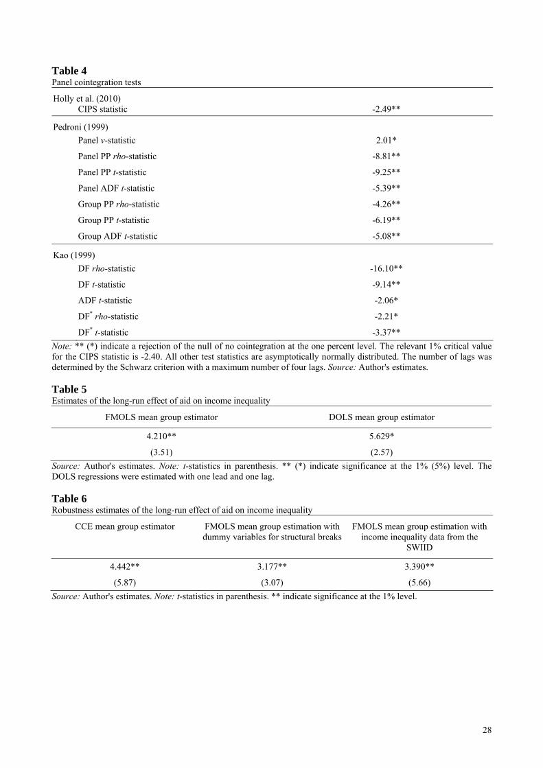
Table 4 Panel cointegration tests

Holly et al. (2010) CIPS statistic -2.49**

Pedroni (1999) Panel ν-statistic 2.01*

Panel PP rho-statistic -8.81**

Panel PP t-statistic -9.25**

Panel ADF t-statistic -5.39**

Group PP rho-statistic -4.26**

Group PP t-statistic -6.19**

Group ADF t-statistic -5.08**

Kao (1999) DF rho-statistic -16.10**

DF t-statistic -9.14**

ADF t-statistic -2.06*

DF* rho-statistic -2.21*

DF* t-statistic -3.37** Note: ** (*) indicate a rejection of the null of no cointegration at the one percent level. The relevant 1% critical value for the CIPS statistic is -2.40. All other test statistics are asymptotically normally distributed. The number of lags was determined by the Schwarz criterion with a maximum number of four lags. Source: Author's estimates. Table 5 Estimates of the long-run effect of aid on income inequality

FMOLS mean group estimator DOLS mean group estimator

4.210**

(3.51)

5.629*

(2.57) Source: Author's estimates. Note: t-statistics in parenthesis. ** (*) indicate significance at the 1% (5%) level. The DOLS regressions were estimated with one lead and one lag. Table 6 Robustness estimates of the long-run effect of aid on income inequality

CCE mean group estimator FMOLS mean group estimation with dummy variables for structural breaks

FMOLS mean group estimation with income inequality data from the

SWIID

4.442**

(5.87)

3.177**

(3.07)

3.390**

(5.66) Source: Author's estimates. Note: t-statistics in parenthesis. ** indicate significance at the 1% level.

28

Figure 1 FMOLS estimation with single country excluded from the sample

Coefficients on Aidit

2.0

2.5

3.0

3.5

4.0

4.5

5.0

5.5

2 4 6 8 10 12 14 16 18 20 No. of omitted country t-statistics of the coefficients

2.0

2.4

2.8

3.2

3.6

4.0

4.4

4.8

2 4 6 8 10 12 14 16 18 20 No. of omitted country

29