the education-innovation gap
TRANSCRIPT

The Education-Innovation Gap*
Barbara Biasi† Song Ma‡
November 14, 2021
Please click here for the most updated version
Abstract
This paper examines whether college and university courses teach frontier knowledge. Compar-ing the text of 1.7 million course syllabi with the abstract of 20 million articles in top scientificjournals at various points in time, we construct the “education-innovation gap,” aimed at cap-turing the distance between each course and frontier knowledge and defined as the averagesimilarity with older articles divided by the average similarity with newer articles. We then doc-ument how the gap varies across and within schools. We find that the gap is lower in schoolsthat spend more, are more selective, and serve fewer disadvantaged and minority students. Thegap is also strongly associated to instructors: it decreases after the instructor of a course changesand it is lower for courses taught by research-active faculty. Lastly, the gap is correlated withstudents’ graduation rates and incomes after graduation. These findings are robust to the use ofalternative measures of course novelty.
JEL Classification: I23, I24, I26, J24, O33
Keywords: Education, Innovation, Syllabi, Instructors, Text Analysis, Inequality
*We thank Jaime Arellano-Bover, David Deming, David Robinson, Kevin Stange, Sarah Turner, and seminar andconference participants at Yale, Duke, Erasmus, Maastricht, Queens, Stockholm School of Economics, NBER (Education;Entrepreneurship; Innovation), AEA, CEPR/Bank of Italy, Junior Entrepreneurial Finance and Innovation Workshop,SOLE, Stanford (Hoover), UCL, IZA TOM and Economics of Education Conferences, and CESifo Economics of EducationConference for helpful comments. Xugan Chen provided excellent research assistance. We thank the Yale Tobin Centerfor Economic Policy, Yale Center for Research Computing, Yale University Library, and Yale International Center forFinance for research support. All errors are our own.
†EIEF, Yale School of Management and NBER, [email protected], +1 (203) 432-7868;‡Yale School of Management and NBER, [email protected], +1 (203) 436-4687.

1 Introduction
In a knowledge-based economy, new ideas and knowledge – non-rival goods with increasing re-
turns – spur technological innovation and are essential to economic growth (Romer, 1990). It is
therefore crucial to understand how ideas and knowledge are produced and disseminated. Educa-
tion systems (particularly higher education ones) play a crucial role as knowledge providers (Biasi
et al., 2020). Given the upward trend in the “burden of knowledge” required to innovate (Jones,
2009), the importance of these programs is likely to grow.
Not all higher education programs, however, are created equal. Just like there is heterogeneity
in the economic returns they produce (Hoxby, 1998; Altonji et al., 2012; Chetty et al., 2019, among
others), there might be differences in the extent to which programs equip students with frontier
knowledge. The goal of this paper is to quantify these differences by examining the content of
higher education instruction. Specifically, we want to measure the distance between the knowledge
content of each course – as described in its syllabus – and the knowledge frontier, represented by
top academic articles recently published in the course’s field.
To quantify this distance, we develop a new metric: the education-innovation gap, designed to cap-
ture the similarity of the content of a course with older knowledge (contained in articles published
decades ago) relative to new, frontier knowledge (contained in recently published articles). For ex-
ample, a Computer Science course that teaches Visual Basic (an obsolete programming language) in
2018 would have a larger gap than a course that teaches Julia (a recent and updated programming
language), because Visual Basic is more frequently covered by old academic articles and Julia is more
frequently covered by recent articles.1
We construct this measure using a “text as data” approach (Gentzkow et al., 2019). Specifi-
cally, we compare the raw text of 1.7 million college and university syllabi, covering about 540,000
courses in 69 different fields taught at nearly 800 US institutions between 1998 and 2018, with the
title, abstract, and keywords of over 20 million academic publications that appeared in top journals
since each journal’s creation. We first represent each document as a binary vector, whose elements
correspond to words of a dictionary and equal one if the document contains the corresponding dic-
1First released by Microsoft in 1991, Visual Basic is still supported by Microsoft in recent software frame-works. However, the company announced in 2020 that the language would not be further evolved(https://visualstudiomagazine.com/articles/2020/03/12/vb-in-net-5.aspx, retrieved September 30th, 2020). Julia is ageneral-purpose language initially developed in 2009. Constantly updated, it is among the best languages for numericalanalyses and computational science. As of July 2021 it was used at 1,500 universities, with over 29 million downloadsand a 87 percent increase in a single year (https://juliacomputing.com/blog/2021/08/newsletter-august/, retrievedSeptember 30, 2021).
1

tionary word (we use set of all words ever listed on Wikipedia as a dictionary). To account for the
importance of a word in the document, its popularity in research at a given point in time, and its use
in the English language we weigh each vector element by the ratio between the word’s frequency
in the document and its frequency in all documents published in previous years (similar to Kelly
et al., 2018).
Using these weighted word vectors, we compute the cosine similarity (a measure of vectorial
proximity) between each syllabus and each article. We then construct the education-innovation gap
of a syllabus as the ratio between the average cosine similarity of a syllabus with articles published
15 years prior and the average similarity with articles published one year prior. By construction, the
gap is higher for syllabi that are more similar to older, rather than newer, knowledge. Importantly,
by virtue of being constructed as a ratio of cosine similarities, the gap is not affected by idiosyncratic
attributes of each syllabus such as length, structure, or writing style.
A few empirical regularities confirm the ability of the education-innovation gap to capture a
course’s distance from the knowledge frontier. First, the gap is strongly correlated with the average
“age” of articles and books listed in the syllabus as required or recommended readings. Second,
graduate-level courses have the smallest gap on average; advanced undergraduate courses have
the second smallest gap, and basic courses – more likely to teach the fundaments of the discipline,
rather than (or in addition to) the latest research – have the largest gap. Third, gradually replacing
“older” knowledge words with “newer” ones, as we do in a simulation exercise, progressively
reduces the gap.
Examining how the education-innovation gap differs across and within schools is helpful to
better understand how the content of higher education is shaped. Multiplying it by 100 for simplic-
ity, the gap is equal to 95 on average: This indicates that courses tend to be more similar to newer
than to older research. However, a significant amount of variation exists across syllabi. Manually
changing the content of each syllabus indicates that, in order to move a syllabus from the 25th per-
centile (92) to the 75th percentile (99) of the distribution, we would have to replace approximately
48 percent of its content with “newer” knowledge, i.e., words that are most frequently found in re-
cent publications. A variance decomposition exercise indicates that differences across schools and
instructors explain 3 and 25 percent of the total variation, highlighting an important role for these
two factors, which we analyze next.
First, we explore whether schools with different characteristics and serving different popula-
tions of students also offer courses with different gaps. Our data indicate that schools with a
2

stronger focus on research, as well as those with higher endowment and expenditures on instruction
and research, have significantly lower gaps. In addition, more selective schools (such as Ivy-Plus,
Chetty et al., 2019) have a lower gap compared to non-selective schools. This difference is such
that, in order to make the average syllabus in non-selective schools comparable to the average for
Ivy-Plus and Elite schools, we would have to replace 8 percent of its content with newer knowledge.
Cross-school differences in the education-innovation gap also imply that access to up-to-date
knowledge is highly unequal among students enrolled in different institutions. In particular, we
find that the gap is negatively related to the economic background of the students at each school,
as measured by median parental income and the share of students whose parental income is in
the top percentile. For example, a one-percent increase in parental median income is associated
with a 0.56 lower gap, which corresponds approximately to a 5 percent difference in the average
syllabus. Similarly, the gap is positively related to the share of students who are Black or Hispanic.
These results indicate that students with a socio-economic advantage, on average, are exposed to
educational content that is closer to the knowledge frontier.
The decomposition exercise also reveals that a larger portion (33 percent) of the total variation
in the gap occurs across, rather than within courses. This implies substantial persistence in the
material that is taught in a given course over time. In line with this, we find that the average gap
of a course is quite stable over time, but it declines substantially when the person who teaches the
course changes, suggesting that instructors who take over a course from someone else update its
content more than instructors who have been teaching the same course for years.
Not all instructors, however, are created equal. The gap declines significantly more when the
new instructor has higher research productivity, measured with academic publications and citations
in the previous five years. Data on public school instructors, for whom we observe job titles and
salaries, further indicate that assistant professors tend to teach courses with the lowest gap, com-
pared to tenured faculty and non-ladder faculty. Regardless of job title, a lower gap is correlated
with a higher instructor salary.
Research-active instructors might be better updated about the frontier of research and more
likely to cover this type of content in their courses, which might result in a lower gap. In line
with this hypothesis, we find that the gap is lower when the instructor’s own interests are closer to
the topic of the course. We also find a negative relationship between the gap and research inputs
available to the instructor, such as the number and size of government grants. These results indicate
that the assignment of instructors to courses can be a powerful tool to expose students to frontier
3

knowledge. They also suggest that public investments in research can generate additional returns
in the form of more updated instruction.
Our results so far indicate significant across- and within-school differences in the extent to which
courses are up-to-date with respect to the knowledge frontiers. Do these differences matter for stu-
dent outcomes? To answer this question, the ideal experiment would randomly allocate students
to courses with different gaps. In the absence of this random variation, we set on the more modest
goal of characterizing the empirical relationship between the education-innovation gap and stu-
dent outcomes, such as graduation rates, incomes after graduation, and intergenerational mobility.
In an attempt to account for endogenous differences across schools, we control for a large set of
school observables such as institutional characteristics, various types of expenditure, instructional
characteristics, enrollment by demographic groups and by major, selectivity, and parental back-
ground. We find that the gap is negatively related to graduation rates and students’ incomes, with
economically meaningful magnitudes. The relationship with intergenerational mobility is instead
indistinguishable from zero.
In the final part of the paper, we probe the robustness of our results to the use of additional mea-
sures of novelty of a course’ content. We consider three measures: the share of all “new” knowledge
contained in a syllabus (designed not to penalize a syllabus that contains old and new knowledge
compared with one that only contains new knowledge); a measure of “tail” knowledge, aimed at
capturing the presence of the most recent content; the education-innovation gap, estimated using
patents as a measure of frontier knowledge instead of academic publications; and a measure of soft
skills, devised to capture the non-academic novelty of a course. All these measures are significantly
correlated with the education-innovation gap, and our main results are qualitatively unchanged
when we use these measures.
This paper contributes to several strands of the literature. First, we characterize heterogeneity
in the production of human capital by proposing a novel approach to measure the content of higher
education. This allows us to relate this content to the characteristics of schools, instructors, and
students, as well as to students’ outcomes. Earlier works have highlighted the role of educational
attainment (Hanushek and Woessmann, 2012), majors and curricula (Altonji et al., 2012), college
selectivity (Hoxby, 1998; Dale and Krueger, 2011), social learning ad interactions (Lucas Jr, 2015;
Lucas Jr and Moll, 2014; Akcigit et al., 2018) and skills (Deming and Kahn, 2018) for labor market
outcomes, innovation, and economic growth. Our analysis focuses instead on the specific concepts
and topics covered in higher education courses, and aims at measuring the extent to which these
4

are up-do-date with respect to the frontier of knowledge.
Second, this paper relates to the literature on the “production” of knowledge. Earlier works
(Nelson and Phelps, 1966; Benhabib and Spiegel, 2005) have highlighted an important role for hu-
man capital and education in the diffusion of ideas and technological advancements. Certain fields,
such as STEM, have been shown to be particularly important for innovation (Baumol, 2005; Toiva-
nen and Vaananen, 2016; Bianchi and Giorcelli, 2019).2 Instead of just looking at differences across
fields, here we take a more “micro” approach, and we quantify differences across courses in the
provision of frontier knowledge, which might be particularly important for growth.
Next, our findings contribute to recent studies on the “democratization” (or lack thereof) of
access to valuable knowledge. For example, Bell et al. (2019) have shown that US inventors (i.e.,
people with at least one patent) come from a small set of top US schools, which admit very few low-
income students. We confirm that these schools provide the most up-to-date educational content,
which in turn suggests that access to this type of knowledge is not equally distributed across the
population.
Lastly, we use of the text of course syllabi as information to characterize the content of higher-
education instruction, relating it to the frontier of knowledge. Similarly to Kelly et al. (2018), who
calculate cosine similarities between the text of patent documents to measure patent quality, and
Gentzkow and Shapiro (2010), who characterize the language of newspaper articles to measure
media slant, we use text analysis techniques to characterize the content of each course and to link it
to frontier technologies. Our approach is similar to Angrist and Pischke (2017), who use hand-coded
syllabi information to study the evolution of undergraduate econometrics classes.
2 Data
Our empirical analysis combines data from multiple sources. These include the text of course syl-
labi; the abstracts of academic publications; salaries, job titles, publications, and grants of each
instructor; information on US higher education institutions; and labor market outcomes for the stu-
dents at these institutions. More detail on the construction of our final data set can be found in the
Online Appendix.
2The literature on the effects of education on innovation encompasses studies of the effects of the land grant collegesystem (Kantor and Whalley, 2019; Andrews, 2017) and, more generally, of the establishment of research universities(Valero and Van Reenen, 2019) on patenting and economic activity.
5

2.1 College and University Course Syllabi
We obtained the raw text of a large sample of college and university syllabi from Open Syllabus
(OS), a non-profit organization which collects these data by crawling publicly-accessible university
and faculty websites.3 The initial sample contains more than seven million English-language syllabi
of courses taught in over 80 countries, dating back to the 1990s until 2019.
Most syllabi share a standard structure. Basic details of the course (such as title, code, and
the name of the instructor) are followed by a description of the content and a list of the required
and recommended readings for each class session. Syllabi also contain information on evaluation
criteria (such as assignments and exams) and general policies regarding grading, absences, lateness,
and misconduct. We extract four pieces of information from the text of each syllabus: (i) basic
course details, (ii) the course’s content, (iii) the list of required and recommended readings, and (iv)
a description of evaluation methods.
Basic course details These include the name of the institution, the title and code of the course,
the name of the instructor, as well as the quarter or semester and the academic year in which the
course is taught (e.g., Fall 2020). Course titles and codes allow us to classify each syllabus into
one of three course levels: basic undergraduate, advanced undergraduate, or graduate. OS assigns
each syllabus to one of 69 detailed fields (examples include English Literature, History, Computer
Science, Economics, and Mathematics; see the Online Data Appendix for the full list of fields).4 We
use this classification throughout the paper. For some tests, we further aggregate fields into four
macro-fields: STEM, Humanities, Social Sciences, and Business.5
Course content We identified the portion of a syllabus that contains a description of the course’s
content by searching for section titles such as “Summary,” “Description,” and “Content.”6 Typically,
this portion describes the basic structure of the course, the key concepts that are covered, and (in
3The Open Syllabus Project was founded at the American Assembly of Columbia University but has been indepen-dent since 2019. The main purpose of the Project is to support educational research and novel teaching and learningapplications.
4The field taxonomy used by OP draws extensively from the 2010 Classification of Instructional Programs of theIntegrated Postsecondary Education Data System, available at https://nces.ed.gov/ipeds/cipcode/default.aspx?y=55.
5Appendix Table AI shows the correspondence between fields and macro-fields.6The full list of section titles used to identify the course description is: “Syllabi”, “Syllabus”, “Title”, “Description”,
“Method”, “Instruction”, “Content”, “Characteristics”, “Overview”, “Tutorial”, “Introduction”, “Abstract”, “Method-ologies”, “Summary”, “Conclusion”, “Appendix”, “Guide”, “Document”, “Module”, “Apporach”, “Lab”, “Back-ground”, “Requirement”, “Applicability”, “Objective”, “Archivement”, “Outcome”, “Motivation”, “Purpose”, “State-ment”, “Skill”, “Competency”, “Performance”, “Goal”, “Outline”, “Schedule”, “Timeline”, “Calendar”, “Guideline”,“Material”, “Resource”, and “Recommend”.
6

many cases) a timeline of the content and the materials for each lecture.
List of readings We compiled a list of bibliographic information for the required and recom-
mended readings of each course by collecting all other in-text citations such as “Biasi and Ma
(2021).” We were able to compile a list of references for 71 percent of all syllabi. We then collected
bibliographic information on each reference from Elsevier’s SCOPUS database (described in more
detail in Section 2.2); this includes title, abstract, journal, keywords (where available), and textbook
edition (for textbooks).
Methods of evaluation To gather information on the methods used to evaluate students and the
set of skills trained by the course, we used information on exams and other assignments. We identi-
fied and extracted the related portion of each syllabus by searching for section titles such as “Exam,”
“Assignment,” “Homework,” “Evaluation,” and “Group.”7 Using the text of these sections, we dis-
tinguished between hard skills (assessed through exams, homework, assignments, and problem
sets) and soft skills (assessed through presentations, group projects, and teamwork). We were able
to identify this information for 99.9 percent of all syllabi.
Sample restrictions and description To maximize consistency over time, we focus our attention
on syllabi taught between 1998 and 2018 in four-year US institutions with at least one hundred
syllabi in our sample.8 We excluded 35,917 syllabi (1.9 percent) with less than 20 words or more
than 10,000 words (the top and bottom 1 percent of the length distribution).
Our final sample, described in panel (a) of Table 1, contains about 1.7 million syllabi of 542,251
courses at 767 institutions. Thirdy-one percent of all syllabi cover STEM courses, 11 percent cover
Business, 30 percent cover Humanities, and 26 percent cover Social Science. Basic courses represent
39 percent of all syllabi and graduate courses represent 33 percent. A syllabus contains an average of
2,226 words in total, with a median of 1,068. Our textual analysis focuses on “knowledge” words,”
i.e., words that belong to a dictionary (see Section 3 for details). The average syllabus contains 420
unique knowledge words.
7The full list of section titles used to identify the skills is as follows: “Exam”, “Quiz”, “Test”, “Examination”, “Final”,“Examing”, “Midterm”, “Team”, “Group”, “Practice”, “Exercise”, “Assignment”, “Homework”, “Evaluation”, “Presen-tation”, “Project”, “Plan”, “Task”, “Program”, “Proposal”, “Research”, “Paper”, “Essay”, “Report”, “Drafting”, “Sur-vey”.
8For consistency, we removed 129,429 syllabi from one online-only university, the University of Maryland GlobalCampus.
7

2.2 Academic Publications
To construct the research frontier in each field and year, we use information from Elsevier’s SCOPUS
database and compile the list of all peer-reviewed articles that appeared in the top academic journals
of each field since the journal’s foundation.9 We define top journals as those ranked among the
top 10 by Impact Factor (IF) in each field at least once since 1975 (or the journal’s creation if it
happened after 1975).10 Our final list of publications includes 20 million articles in the same fields as
our syllabi, corresponding to approximately 100,000 articles per year.11 We capture the knowledge
content of each article with its title, abstract, and keywords.
Alternative measure of knowledge: Patents An alternative way to measure the knowledge fron-
tier is to use the text of patents, rather than academic publications. To this purpose we collected
data on the text of more than six million patents issued since 1976 from the USPTO website.12 We
capture the content of each patent with its abstract.
2.3 Instructors: Research Productivity, Funding, Job Title, and Salary,
Nearly all course syllabi report the name of the course instructor. Using this information, we col-
lected data on instructors’ research productivity (publications and citations) and the receipt of pub-
lic research funding. For a subset of instructors, we also collected information on job titles and
annual salary.
Research Productivity Publications and citations data come from Microsoft Academic (MA), a
search engine that lists publications, working papers, other manuscripts, and patents for each listed
researcher, together with the counts of citations to these documents. We searched MA for the name
of each syllabus instructor and their institution; when the search was successful, we linked the syl-
labus to the corresponding MA record. We are able to successfully find 33 percent of all instructors,
and we assume that the instructors we could not find never published any article (Table 1, panel
(b)).9We access the SCOPUS data through the official API in April-August 2019.
10Even if a journal appeared only once in the top 10, we collect all articles published since its foundation.11SCOPUS classifies articles into 191 fields. To map each of these to the 69 syllabi fields, we calculate the cosine
similarity (see Section 3) between each syllabus and each article. We then map each syllabi field with the SCOPUSfield with the highest average similarity. Details on the mapping of fields between the syllabi and SCOPUS articles arecontained in the Data Appendix.
12Our web crawler collected the text content of all patents (in HTML format) from http://patft.uspto.gov/netahtml/PTO/srchnum.htm, with patent numbers ranging from 3850000 to 10279999).
8

Using data from MA, we measure each instructor’s research quantity and quality with the num-
ber of publications and the number of citations received in the previous five years.13 On average,
instructors published 5.5 articles in the previous five years, with a total of 125 citations (Table 1,
panel (b)). The distributions of citation and publication counts are highly skewed: The median
instructor in our sample only published one article in the previous five years and received no cita-
tions.
Funding We complement publications data from MA with information on government grants
received by each researcher. Beyond research productivity, this information allows us to measure
public investment in academic research. We focus on two among the main funding agencies of
the U.S. government: the National Science Foundation (NSF) and the National Institute of Health
(NIH).14 Our grant data include 480,633 NSF grants active between 1960 and 2022 (with an average
size of $582K in 2019 dollars, Table 1, panel (b)) and 2,566,358 NIH grants active between 1978 and
2021 (with an average size of $504K). We link grants to syllabi via a fuzzy matching between the
names of the grant investigators (PIs and co-PIs) and the name of the instructors (more detail can
be found in the Data Appendix). Eleven percent of all syllabi instructors are linked to at least one
grant; among these, the average instructor receives 14 grants with an average size of $5,224K.
Job Title and Salary In many U.S. states, salaries of public college and university employees are
public information, to comply with state regulations on transparency and accountability. These
records are usually disclosed online, together with each employee’s name and job title. We were
able to collect information on salaries and job titles for 35,178 instructors in our syllabi sample
(10.6 percent of all instructors and 14.3 percent of public-sector instructors), employed in 490 public
institutions in 16 states. We observe an average of two years’ worth of salary for each employee (the
modal year is 2017). We detail the coverage of the salary data in the Online Appendix.
Among all syllabi instructors for which we have job title information, 42 percent are ladder fac-
ulty (including 11 percent of assistant professors, 13 percent of associate professors, and 18 percent
of full professors; Appendix Figure AI, panel (a)). Instructors earn $80,388 on average, although
large variation in pay exists between job titles. Conditional on field, course level, and year, ad-
junct professors and lecturers earn $63,396; clinical and practice professors earn $119,685; assistant,
13Using citations and publications in the previous five years helps address issues related to the life cycle of publica-tions and citations, with older instructors having a higher number of citations and publications per year even if theirproductivity declines with time.
14These data are published by each agency, at https://www.nsf.gov/awardsearch/download.jsp and https://exporter.nih.gov/ExPORTER_Catalog.aspx. We accessed these data on May 25, 2021.
9

associate, and full professors earn $85,261, $97,766, and $128,589 (Appendix Figure AI, panel (b)).15
2.4 Information on US Higher Education Institutions
The last component of our dataset includes information on all US colleges and universities of the
syllabi in our data. Our primary source is the the Integrated Postsecondary Education Data Sys-
tem (IPEDS), maintained by the National Center for Education Statistics (NCES).16 For each school,
IPEDS reports a set of institutional characteristics (such as name and address, control, affiliation,
and Carnegie classification); the types of degrees and programs offered; expenditure and endow-
ment; characteristics of the student population, such as the distribution of SAT and ACT scores of
all admitted students, enrollment figures for different demographic groups, completion rates, and
graduation rates; and faculty composition (ladder and non-ladder).We link each syllabus to the cor-
responding IPEDS record via a fuzzy matching algorithm based on school names. We are able to
successfully link all syllabi in our sample.
We complement data from IPEDS with information on schools and students from two additional
sources. The first one is the dataset assembled and used by Chetty et al. (2019), which includes a
school’s selectivity tier (defined using Barron’s scale), the incomes of students and parents, and
measures of intergenerational mobility (such as the share of students with parental income in the
bottom quintile who have incomes in the top quintile as adults, calculated using data on US tax
records). The second is the College Scorecard Database of the US Department of Education, an
online tool designed to help users compare costs and returns of attending various colleges and
universities in the US. This database reports the incomes of graduates ten years after the start of the
program. We use these variables, available for the academic years 1997-98 to 2007-08, to measure
student outcomes for each school.
Panel (c) of Table 1 summarizes the sample of colleges and universities for which we have syllabi
data. The median parental income at these schools is $97,917 on average. Across all schools, 3
percent of all students have parents with incomes in the top percentile. The share of minority
students is equal to 0.22, with a standard deviation of 0.17. Graduation rates average 61.4 percent in
2018, whereas students’ incomes ten years after school entry, for the 2003–04 and 2004–05 cohorts,
are equal to $45,035. Students’ intergenerational mobility, defined as the probability that students
15Panel (b) of Appendix Figure AI displays point estimates and confidence intervals of indicators for job titles in anOLS regression of salaries (expressed in $1,000), controlling for field-by-course level-by-year fixed effects. We clusterstandard errors at the instructor level).
16IPEDS includes responses to surveys from all postsecondary institutions since 1993. Completing these surveys ismandatory for all institutions that participate, or apply to participate, in any federal financial assistance programs.
10

from the bottom quintile of parental income reach the top income quintile during adulthood, is
equal to 0.29 on average.
2.5 Data Coverage and Sample Selection
Our syllabi sample corresponds to only a small fraction of all courses taught in US schools between
1998 and 2018. The number of syllabi increases over time, from 17,479 in 2000 to 68,792 in 2010 and
190,874 in 2018 (Appendix Figure AII).
To more accurately interpret our empirical results, it is crucial to establish patterns of selection
into the syllabi sample. To do so, we compiled the full list of courses offered between 2010 and 2019
in a subsample of 161 US institutions (representative of all institutions included in IPEDS) using the
course catalogs in the archives of each school.17 This allows us to compare our syllabi sample to the
population of all courses for these schools and years.
First, we show that the share of catalog courses covered by the syllabi sample remained stable
over time, at 5 percent (Appendix Figure AV). This suggest that, at least among the schools with
catalog information, the increase in the number of syllabi over time is driven by an increase in the
number of courses that are offered, rather than an increase in sample coverage.
Second, we show that our syllabi sample does not disproportionally cover courses in certain
fields or levels. In 2018, STEM courses represent 32 percent of syllabi in our sample and 24 percent of
courses in the catalog; Humanities represent 25 and 31 percent, and Social Sciences represent 21 and
19 percent, respectively (Appendix Figure AIII). Similarly, basic undergraduate courses represent 40
percent of syllabi in our sample and 31 percent of courses in the catalog; advanced undergraduate
courses represent 26 and 30 percent, and graduate courses represent 33 and 38 percent (Appendix
Figure AIV). These shares are fairly stable over time.
Lastly, we show that a school’s portion of the catalog that is included in our sample and the
change in this portion over time are not systematically related to school observables. In Panel (a)
of Table 2 (column 1) we regress a school’s share of courses included in our sample in 2018 on the
following variables, one at the time and also measured in 2018: financial attributes (such as ex-
penditure on instruction, endowment per capita, sticker price, and average salary of all faculty),
enrollment, the share of students in different demographic categories (Black, Hispanic, alien), and
the share of students graduating in Arts and Humanities, STEM, and the Social Sciences. We also17We begin by randomly selecting 200 schools among all 4-year IPEDS institutions. Among these, we were able to
compile course catalogs for 161 institutions, listed in Appendix Table AII. These look very similar in terms of observablesto all schools in our sample (Appendix Table AIII). We focus our attention on years from 2010 to maximize our coverage.For an example of a course catalogue, see https://registrar.yale.edu/course-catalogs.
11

estimate the joint significance of all these variables together. This exercise indicates that these vari-
ables are individually and jointly uncorrelated with the share of courses in the syllabi sample, with
an F-statistic smaller than one. In column 2 we repeat the same exercise, using the 2015-2018 change
in the share of courses included in the syllabi as the dependent variable. Our conclusions are un-
changed.
The only dimension in which our syllabi sample appears selected is school selectivity. Relative
to non-selective institutions (for whom the share of courses in the sample is less than 0.1 percent),
Ivy-Plus and Elite schools have a 0.9 percentage point higher share of courses included in the syllabi
sample, and selective public schools have a staggering 4.5 percent higher share.
Taken together, these tests indicate that our syllabi sample does not appear to be selected on the
basis of observable characteristics of schools and fields, although it does over-represent Ivy-Plus
and Elite and selective public schools. By construction, though, we cannot test for selection based
on unobservables. Our results should therefore be interpreted with this caveat in mind.
3 Measuring the Education-Innovation Gap
To construct the education-innovation gap we combine information on the content of each course,
captured by its syllabus, with information on frontier knowledge, captured by academic publica-
tions. We now describe the various steps for the construction of this measure, provide the intuition
behind it, and perform validation checks.
Step 1: Measuring Similarities in Text
To construct the gap, we begin by computing textual similarities between each syllabus and each
academic publication. To this purpose, we represent each document d (a syllabus or an article) in the
form of a vector Vd of length |W |, whereW is the set of unique words in a given language dictionary
(we define dictionaries in the next paragraph). Each element w of Vd equals one if document d
contains word w ∈ W . To measure the textual proximity of two documents d and k we use the
cosine similarity between the corresponding vectors Vd and Vk:
ρdk =Vd
‖Vd‖· Vk
‖Vk‖
In words, ρdk measures the proximity of d and k in the space of words W . To better capture the
distance between the knowledge content of each document (rather than simply the list of words),
12

we make a series of adjustments to this simple measure, which we describe below.
Accounting for term frequency and relevance Since our goal is to measure the knowledge con-
tent of each document, we assign more weight to terms that best capture this type of content rel-
ative to terms that are used frequently in the language (and, as such, might appear often in the
document) but do not necessarily capture content. To this purpose, we use the “term-frequency-
inverse-document-frequency (TFIDF)” transformation of word counts, a standard approach in the
text analysis literature (Kelly et al., 2018). This approach consists in comparing the frequency of each
term in the English language and in the body of all documents of a given type (e.g., syllabi or arti-
cles), assigning more weight to terms that appear more frequently in a given document than they
do across all documents. For example, “genome editing” is used rarely in the English language,
but often in some Biology syllabi; “assignment” is instead common across all syllabi. Because of
this, “genome editing” is more informative of the content of a given syllabus and should therefore
receive more weight than “assignment”.
The TFIDF weight of a term w in document d is:
TFIDFwd = TFwd × IDFw
where cwd counts the number of times term w appears in d, TFwd ≡ cwd∑k∈W ckd
is the frequency of
word w in document d, and
IDFw ≡ log
(|D|∑
n∈D 1(w ∈ Vd)
)
is the inverse document frequency of term w in the set D of all documents of the same type as d.
Intuitively, the weight will be higher the more frequently w is used in document d (high TFwd),
and the less frequently it is used across all documents (low IDFd). In words, words that are more
distinctive of the knowledge content of a given document will receive more weight.
To maximize our ability to capture the knowledge content of each document, in our analysis
we focus exclusively on words related to knowledge concepts and skills, excluding words such as
pronouns or adverbs. We do this by appropriately choosing our “dictionaries,” lists of all relevant
words (or sets of words) that are included in the document vectors. Our primary dictionary is the
list of all unique terms ever used as keywords in academic publications from the beginning of our
publication sample until 2019. As an alternative, we have also used the list of all terms that have an
English Wikipedia webpage as of 2019; our results are robust to this choice.
13

Accounting for changes in term relevance over time The weighting approach described so far
calculates the frequency of each term by pooling together documents published in different years.
This is not ideal for our analysis, because the resulting measures of similarity between syllabi and
publications would ignore the temporal ordering of these documents. Instead, we are interested
in the novelty of the content of a syllabus d relative to research published in the years prior to d,
without taking into account the content of future research. To see this consider, for example, course
CS229 at Stanford University, taught by Andrew Ng in the early 2000 and one of the first entirely
focused on Machine Learning. Pooling together documents from different years would result in a
very low TFIDFwd for the term “machine learning” in the course’s syllabus: Since the term has
been used very widely in the last years, its frequency across all documents would be very high and
its IDF very low. Not accounting for changes in the frequency of this term over time would then
lead us to misleadingly underestimate the course’s path-breaking content.
To overcome this issue, we modify the traditional TFIDF approach and construct a retrospec-
tive or “point-in-time” version of IDF , meant to capture the inverse frequency of a word among all
articles published up to a given date. We call this measure “backward-IDF ,” or BIDF , and define it
as
BIDFwt ≡ log
( ∑d 1(t(d) < t)∑
d 1(t(d) < t)× 1(w ∈ Vd)
)
where t(d) is the publication year of document d. Unlike IDF , BIDF varies over time to capture
changes in the frequency of a term among documents of a given type. This allows us to give the term
its temporally appropriate weight. Using the BIDF we can now calculate a “backward” version of
TFIDF , substituting BIDF to IDF :
TFBIDFwd = TFwd ×BIDFwt(d)
Building the weighted cosine similarity Having calculated weights TFBIDFwd for each term w
and document d, we can obtain a weighted version of our initial vector Vd, denoted as Vd, multi-
plying each term w ∈ Vd by TFBIDFwd. We can then re-define the cosine similarity between two
documents d and k, accounting for term relevance, as
ρdk =Vd‖Vd‖
· Vk‖Vk‖
.
Since TFBIDFwd is non-negative, ρdk lies in the interval [0, 1]. If d and k are two documents of
14

the same type that use the exact same set of terms with the same frequency, ρdk = 1; if instead they
have no terms in common, ρdk = 0.
3.1 Calculating the Education-Innovation Gap
To construct the education-innovation gap, we proceed in 3 steps.
Step 1: We calculate ρdk between each syllabus d and article k.
Step 2: For each syllabus d, we define the average similarity of a syllabus with all the articles
published in a given three-year time period τ :
Sτd =∑
k∈Ωτ (d)
ρdk
where ρdk is the cosine similarity between syllabus d and a article k (defined in equation (3)) and
Ωτ (d) is the set of all articles published in the three-year time interval [t(d)− τ − 2, t(d)− τ ].18
Step 3: We construct the education-innovation gap as the ratio between the average similarity of a
syllabus with older technologies (published in τ ) and the similarity with more recent ones (τ ′ < τ ):
Gapd ≡(SτdSτ′d
)(1)
It follows that a syllabus published in t has a lower education-innovation gap if its text is more
similar to more recent research than older research. In our analysis, we set τ = 13 and τ ′ = 1, and
we scale the measure by a factor of 100 for readability.
It is worth emphasizing the advantage of a ratio measure over a simple measure of similarity
(S1d). In particular, the latter could be sensitive to idiosyncratic differences in the “style” of language
across syllabi in different fields, or even within the same field. A ratio of similarity measures for the
same syllabus is instead free of any time-invariant, syllabus-specific attributes.
3.2 Validation and Interpretation of Magnitudes
To gauge the extent to which the education-innovation gap is able to capture the “novelty” of a
course’s content, we perform a series of checks. First, we show that the relationship between the
gap and the average age of its reference list (defined as the difference between the year of each
syllabus and the publication year of each reference) is quite strong and almost linear (Figure 1,
panel (a)).
18For our main analysis we use three-years intervals; our results are robust to the use of one-year or two-years intervals.
15

Second, we show that more advanced and graduate courses have a lower gap compared with
basic undergraduate courses. Controlling for field-by-year effects, the latter have a gap of 95.7;
more advanced undergraduate courses have a gap of 95.3, and graduate courses have a gap of 94.7
(Appendix Figure 1, panel (b)). This suggests that more advanced courses cover content that is
closer to frontier research.
Third, we simulate how changing the content of a course translates into changes in the education-
innovation gap. Specifically, we progressively replace “old” words with “new” words in a ran-
domly selected subsample of 100,000 syllabi and re-calculate the gap for each syllabus as we replace
more words. New words as those in the top 5 percent in terms of frequency in the new publication
corpus between t-3 and t-1 or in the new publication corpus between t-3 and t-1 but not in the old
publication corpus between t-15 and t-13; old words are those in the top 5 percent in terms of fre-
quency in the old publication corpus between t-15 and t-13 or in the old publication corpus between
t-15 and t-12 but not in the new publication corpus between t-3 and t-1. This exercise shows that
the gap monotonically decreases as we replace old words with new ones (Figure 1, panel (c)). This
simulation is also useful to gauge the economic magnitude of changes in the gap. In particular, a
unit change in the gap requires replacing 10 percent of a syllabus’s old words (or 34 old words,
compared with 331 words for the median syllabus).
Lastly, we demonstrate that our measure performs well in capturing the extent to which a syl-
labus contains old and new knowledge. We do so by constructing a set of 1.7 million fictitious
syllabi as sets of knowledge words, each with a given ratio of old to new words, and calculating the
education-innovation gap for each of them. The gap is strongly related with the ratio of old to new
words, with a correlation of 0.96 (Figure 1, panel (d)).19
3.3 The Education-Innovation Gap: Variation and Variance Decomposition
The average course has a gap of 95.3, with a standard deviation of 5.8, a 25th percentile of 91.6, and
a 75th percentile of 98.8; the distribution is shown in Appendix Figure AVI. To give an economic
meaning to this variation, we make use of the relationship illustrated in panel (c) of Figure 1. In
order to move a syllabus from the 75th to the 25th percentile of the distribution (a change in the gap
of 7.2) we would have to replace approximately 200 of its words, or 48 percent of the content of the
average syllabus (which contains 420 words).
To better understand whether the variation in the gap occurs across schools, within schools and
19This simulation is described in greater detail in the Online Data Appendix.
16

across courses, or rather within courses over time, we perform an analysis of the variance using the
Shapley-Owen decomposition, and decompose the total variation in the gap into a set of factors.
For each factor j, we calculate the partial R2 as
R2j =
∑k 6=j
R2 −R2(−j)K!/j!(K − j − 1)!
where R2(−j) is the R2 of a regression that excludes factor j. We consider five factors: year, field,
school, course, and instructor, and we use adjusted R2 throughout to account for the large number
of fixed effects in the model.
Partial R2s, shown in Table 3 (column 1), indicate that fields explain 4 percent of the total vari-
ation in the gap, while schools explain 2 percent. Courses explain a large 33 percent, indicating
a great deal of persistence in the content of a course over time. Importantly, instructors explain a
large 25 percent. In column 2, we obtain similar exercises when substituting courses with course
levels. In the remainder of the paper, we focus more in depth on two of these factors: institutions
and instructors. Specifically, we study how the gap varies across different types of schools serving
different populations of students, and we explore how it relates to the research productivity and
focus of the person who teaches the course.
4 The Education-Innovation Gap Across Schools
The decomposition exercise indicates that differences across schools explain approximately 2 per-
cent of the total variation in the gap. Albeit small, cross-school differences might reflect disparities
in access to frontier knowledge among students with different backgrounds, if schools with differ-
ent gaps also serve different student populations. To assess this, we explore whether the education-
innovation gap is related to the characteristics of each school and the students they serve.
4.1 School Characteristics
We begin by testing how the education-innovation-gap relates to three sets of school attributes: (i)
institutional, such as the sector (public or private), the research intensity (distinguishing between
schools classified as R1 – “Very High Research Intensity” – according to the Carnegie classifica-
tion, and all other schools) and the emphasis on liberal arts and sciences relative to other subjects
(distinguishing between Liberal Arts Colleges (LAC) and all other schools); (ii) financial, such as
endowment and spending on instruction, faculty salaries, and research; (iii) and faculty, such as
17

the share of non-ladder faculty, the share of tenure-track (non-tenured) faculty, and the number of
academic publications per faculty.
We estimate pairwise correlations between the gap and these attributes accounting for field,
course level, and year of the syllabus using the following specification:
Gapi = Xiβ + φf(i)l(i)t(i) + εi,
where Gapi measures the education-innovation gap of syllabus i, taught in school s(i) in year t(i);
the variable Xi is the institutional characteristic of interest; and field-by-level-by-year fixed effects
φflt control for systematic, time-variant differences in the gap that are common to all syllabi in the
same field and course level. We cluster standard errors at the institution level.
Estimates of β for each school characteristic, shown in Figure 2, indicate that public schools have
a slightly higher gap compared with non-public schools, but this difference is indistinguishable
from zero. No differences appear between LACs and other schools; R1 schools have instead a 0.2
lower gap compared with schools with a lower research intensity.
In order to quantify the economic magnitude of the difference in gaps between R1 and other
schools, we can again use the simulation results in Figure 1 (panel c). In order to close the difference
in the gap between R1 and other schools, we would have to replace approximately 2 percent of
the knowledge content of the average syllabus (7 terms). The difference between R1 and other
institutions, although significant, is therefore quite small.
A statistically and economically significant relationship exists between the gap and financial
characteristics, such as endowment and spending on instruction, faculty salary, and research. For
example, a 10-percent increase in instructional spending is associated with a 3.5 lower gap, or a 35
percent change in the syllabus; a 10-percent increase in research spending is associated with a unit
lower gap or a 10 percent change in the syllabus.
4.2 Selectivity
Next, we test whether the gap is related to the average ability of across schools that admit different
shares of their applicants. Following Chetty et al. (2019), we bin schools in four “tiers” according
to their selectivity in admissions, as measured by Barron’s 2009 ranking. “Ivy Plus” include Ivy
League universities and the University of Chicago, Stanford, MIT, and Duke. “Elite” schools are all
the other schools classified as tier 1 in Barron’s ranking. “Highly selective” schools include those
in tiers 2 and 3, while “Selective” schools are those in tiers 4 and 5. Lastly, “Non-selective” schools
18

include those in Barron’s tier 9 and all four-year institutions not included in Barron’s classification.20
To compare the gap across different school tiers, we use the following equation:
Gapi = S′iβ + φf(i)l(i)t(i) + εi,
where the vector S′i contains indicators for selectivity tiers (we omit non-selective schools), and
everything is as before.
Point estimates of the coefficients vector β in equation (2), shown as diamonds in Figure 2,
capture the difference in the gap between schools in each tier and non-selective schools. These
estimates indicate that Ivy Plus and Elite schools have the smallest gap, -0.84 smaller than non-
selective schools (corresponding to an 8 percent difference in the average syllabus). Highly selective
schools have a -0.67 smaller gap (6 percent) compared with non-selective schools, and selective
schools have a -0.51 percent smaller gap (5 percent).
These estimates indicate that more selective schools, who enroll students with higher ability,
offer content that is closer to the research frontier. A possible interpretation for these differences is
that more selective schools offer higher-quality education. However, if higher-ability students are
better able to absorb newer content, an alternative interpretation is that schools tailor instruction to
the abilities of their students. We attempt to test this hypothesis in Section 6, where we relate the
education-innovation gap to student outcomes.
4.3 Students’ Characteristics
Schools with different characteristics serve different populations of students; for example, Ivy-Plus
and Elite schools are disproportionately more likely to enroll students from wealthier backgrounds
(Chetty et al., 2019). Cross-school differences might therefore translate into significant disparities
in access to up-to-date knowledge among students with different backgrounds. Here, we focus on
two dimensions of socio-economic backgrounds: parental income and race and ethnicity.
Parental income To establish a relationship between the education-innovation gap and parental
income of students enrolled at each school, we re-estimate equation (2) using two measures of
income as the explanatory variable: Median parental income and the share of parents with incomes
in the top percentile of the national distribution, constructed using tax returns for the years 1996 to
2004 (Chetty et al., 2019). These estimates, shown as the full triangles in the bottom panel of Figure 2,
20For comparability, we exclude two-year institutions.
19

indicate that schools serving more economically disadvantaged students offer courses with a lower
gap. Specifically, a one-percent increase in parental median income is associated with a 0.56 lower
gap, which corresponds approximately to a 5 percent difference in the average syllabus. Similarly,
an increase in the share of students with parental income in the top percentile from 0.01 to 0.10 is
associated with a 0.42 lower gap, or a 4 percent difference in the average syllabus syllabus.
Importantly, these relationships are not driven by students’ ability. Controlling for the average
SAT score of students admitted at each school yields estimates (shown as the hollow triangles in the
bottom panel of Figure 2) which are only slightly smaller than the baseline.
Students’ race and ethnicity Schools that enroll a higher share of minority students (defined as
those who are either Black or Hispanic) also tend to have a higher gap. Using the share of minority
students as the explanatory variable in equation (2) reveals that a one-percentage point increase in
the share of minority students at each school is associated with a 0.58 higher gap, equivalent to a 6
percent change in the average syllabus. As before, this relationship holds if we control for average
student ability.
In line with existing evidence on disparities in access to selective schools among more and less
advantaged students, our results document a new dimension of inequality: That in access to educa-
tional content that is close to the research frontier. Importantly, this inequality cannot be explained
by differences in ability.
5 Evolution of Syllabi Content Over Time and The Role of Instructors
Our decomposition indicates that courses and instructors explain most of the variation in the gap.
This in turn suggests that (i) there is a lot of persistence in a course’s material over time and (ii)
instructors play a significant role in shaping the content of the courses that they teach. We now
explore these two results more in depth. First, we document how the content of a course changes
over time and, in particular, how it changes after an instructor change. Second, we relate the aver-
age education-innovation gap of a course with instructor characteristics such as job title, research
productivity, and fit with the course topic. We end by relating the gap to instructors’ pay.
5.1 The Education-Innovation Gap When The Instructor Changes
We begin by studying how the content of an existing course changes when a new instructor takes
over. We estimate an event study of the gap in a 8-years window around the time of the instructor
20

change:
Gapi =
4∑k=−4
δk1(t(i)− Tc(i) = k) + φc(i) + φf(i)t(i) + εi, (2)
where i, c, f , and t denote a syllabus, course, field, and year respectively, and the variable Tc repre-
sents the first year in our sample in which the instructor of course c changed.21 To minimize error,
we restrict our attention to courses taught by a maximum of two instructors in each year and we
set t(i)− Tc = 0 for all courses without an instructor change, which serve as the comparison group.
We cluster our standard errors at the course level. In this equation, the parameters δk capture the
differences between the gap k years after an instructor change relative to the year preceding the
change.
OLS estimates of δk, shown in Figure 3, indicate that a change in a course’s instructor is associ-
ated with a sudden decline in the education-innovation gap. Estimates are indistinguishable from
zero and on a flat trend in the years leading to an instructor change; the year of the change, the gap
declines by 0.1. This decline is equivalent to replacing 2 percent of the content of a syllabus, or 8
knowledge words.
In Table 4 (panel a) we re-estimate equation (2) for different subsamples of syllabi, pooling to-
gether years preceding and following an instructor change. After a change, the gap declines for
all fields and course levels by about 0.1 on average (8 additional words or 2 percent of a course’s
content, column 1, significant at 1 percent). The decline is largest for Humanities (-0.12) and STEM
courses (-0.1; columns 3 and 4, respectively), as well as for and graduate courses (-0.11, column 8).
These results confirm that instructors play a crucial role in shaping the content of the courses
they teach. They also suggest that, while instructors who teach the same course over multiple years
tend to leave the content unchanged, those who take over an existing course from someone else
significantly update the material, bringing it closer to the knowledge frontier.
5.2 The Education-Innovation Gap and Instructors’ Characteristics
The decline in the gap that follows an instructor change could mask substantial differences across
instructors. For example, the decline could be larger for instructors who are more research-active,
and thus better informed about frontier knowledge. Similarly, it could be larger if the new instructor
is an expert on the topics covered by the course, i.e., if their research interests are in line with the
course. We now explore these possibilities.
21Our results are robust to using the median or last year of the instructor change.
21

Ladder vs non-ladder faculty Ladder (i.e., tenure-track or tenured) faculty are generally more
focused on research compared with non-ladder faculty, whose primary job isto teach. If research
activity matters for the content of a course, we might see differences among ladder and non-ladder
faculty. Averages of the education-innovation gap by job title, controlling by field-by-course level-
by-year effects, indicate that non-ladder faculty – and specifically adjunct professors – have the
largest gap, at 95.8 (Figure 4). Tenure-track assistant professors, on the other hand, have the lowest
gap at 95. The difference between assistant and adjunct professors is equivalent to 30 words, or 7
percent of a syllabus’s content.
Notably, the gap is almost as high for full (tenured) professors as it is for adjuncts, at 95.6.
Associate professors have a slightly smaller gap than full at 95.5, but still significantly higher than
assistant professors. Younger faculty on the tenure track thus appear to teach the courses with the
most updated content.
Research productivity One possible explanation for these results is that assistant professors are
more active in research, and thus more informed on the knowledge frontier. We test this hypothesis
directly by exploring the relationship between a course’s gap and the research productivity of the
instructor, measured using individual counts of citations and publications in the previous five years.
Panels (a) and (b) of Figure 5 show a binned scatterplot of the gap and either citations (panel a)
or publications (panel c) in the prior 5 years, controlling for field effects.22 The relationship between
the gap and instructors’ productivity is significantly negative for both measures of productivity.
This negative relationship is confirmed by the estimates in Table 5 (column 1), where we express
the education-innovation gap (measured at the course-year level) as a function of within-field quar-
tiles of instructor publications (panel a) and citations (panel b); the omitted category are courses
whose instructors do not have any publications or citations. In these specifications we control for
course and field-by-year fixed effects, to account for unobserved determinants of the gap that are
specific to a course in a given field and year. These estimates are thus obtained off of changes in
instructors for the same course over time. The gap progressively declines as the number of instruc-
tor publications and citations grows. In particular, a switch from an instructor without publications
and one with a number of publications in the top quartile of the field distribution is associated with
a 0.11 decline in gap (equivalent to changing 8 words or 2 percent of a course’s syllabus; Table 5,
panel (a), column 1, significant at 1 percent). Similarly, a switch from an instructor without citations
22In this figure, the horizontal axis corresponds to quantiles of each productivity measures; the vertical axis shows theaverage gap in each quantiles.
22

to one with citations in the top quartile is associated with a 0.06 lower gap (panel b, column 1, sig-
nificant at 5 percent). These relationships are stronger for Social Science courses (column 5) and for
courses at the graduate level (column 8).
Fit between the instructor and the course These findings indicate that instructors who produce
more and better cited research teach courses with a lower gap. A possible explanation for this
finding is that research-active instructors are better informed about the research frontier. If this is
the case, we should expect this relationship to be stronger for courses that are closer in terms of
topics to the instructor’s own research.
To test for this possibility, we construct a measure of “fit” between the course and the instruc-
tor’s research, defined as the cosine similarity between the set of all syllabi from the same course
across schools and the instructor’s research in the previous 5 years.23 One attractive property of this
measure is that it is does not uniquely reflect the content of the syllabus itself, which is of course
directly shaped by the instructor; rather, it aims at capturing the content of all courses on the same
topic. We then correlate this measure with the education-innovation gap, controlling for course
and field-by-year fixed effects. Estimates of this relationship indicate that a one-standard deviation
increase in instructor-course fit is associated with a 0.09 decline in the gap (Table 8, significant at
5 percent). This relationship is particularly strong for STEM and Social Science (column 4) and for
courses at the advanced undergraduate level (column 6).
Research funding Our results so far indicate a positive relationship between research output and
the education-innovation gap. We now test whether the same relationship holds for research inputs,
such as government grants. Data on the number of NSF and NIH grants received by each instructor
reveals a negative relationship between the gap and these two measures of research inputs (Figure 5,
panel d).
This relationship is confirmed by the estimates in Table 7. Controlling for course and field-by-
year effects, a switch from an instructor who never received a grant to one with at least one grant
is associated with a 0.05 reduction in the gap (column 1, significant at 5 percent). This suggest that
public investments in academic research can yield additional private and social returns in the form
of more up-to-date instruction.
23Constructing this measure requires obtaining a unique identifier for courses on the same field or topic (e.g. MachineLearning) across schools. The Online Appendix details the procedure we use to perform this.
23

Salaries Lastly, we investigate whether instructors who teach more updated content are compen-
sated for it in the form of higher salaries. We estimate the following specification:
Gapi = γ lnwk(it)t + φf(i)l(i)t(i) + εi
where wkt is the salary of instructor k in year t. Estimates of γ indicate that a 10-percent higher
salary is associated with a -0.5 lower gap, equivalent to a change in the syllabus of X (column 1,
significant at 1 percent). This estimate remains robust when we control for school fixed effects.
When we control for job title, however, the estimate of γ becomes smaller and insignificant from
zero (column 3). This indicates that the relationship between pay and the gap is largely driven by
adjunct faculty having the lowest salary and the highest gap.
Taken together, the findings in this section outline an important role for instructors in shaping
the content of the course they teach. Research-active instructors are particularly likely to cover
frontier knowledge in their courses. This suggests that a well-thought assignment of instructors to
courses can be a valuable tool to ensure students are exposed to up-to-date content.
6 The Education-Innovation Gap and Students’ Outcomes
We have shown that significant differences in access to up-to-date knowledge across schools serving
different types of students and across courses within the same school. We now study whether
these differences are related to students’ outcomes. We focus on three outcomes: graduation rates,
income, and intergenerational mobility. Graduation rates are from IPEDS and cover the years 1998
to 2018. Data on students’ incomes ten years after graduation are from the College Scorecard, and
cover students who graduated between 1998 and 2008. We complement this information with cross-
sectional data on average and median incomes and the odds of reaching top income percentiles of
all students who graduated from each school between 2002 and 2004, calculated by Chetty et al.
(2019) using data from tax records. Chetty et al. (2019) also provide a measure of intergenerational
mobility, defined as the probability that students with parental incomes in the bottom quintile of
the distribution reach the top quintile during adulthood.
All these outcomes are measured at the school level, whereas the education-innovation gap is at
the syllabus level. To construct a school-level measure we follow the school value-added literature
(see Deming, 2014, for example) and estimate the school component of the gap using the following
model:
24

Gapi = θs(i) + φf(i)l(i)t(i) + εi. (3)
In this equation, the quantity θs captures the average education-innovation gap of school s, ac-
counting flexible time trends that are specific to the level l and the field f of the course. Because
outcome measures refer to students who complete undergraduate programs at each school, we con-
struct θs using only undergraduate syllabi; our results are robust to the use of all syllabi. Appendix
Figure AIX shows the distribution of θs; the standard deviation is 0.85, corresponding to a 5 percent
change in the average syllabus.
In the remainder of this section, we present estimates of the parameter δ in the following equa-
tion:
Yst = δθzs +Xstγ + τt + εst (4)
where Yst is the outcome for students who graduated from school s in year t, θzs the school fixed
effect in equation (3) standardized to have mean zero and variance one, Xst is a vector of school
observables, and τt are year fixed effects. We calculate bootstrapped standard errors, clustered at
the level of the school, to account for the fact that θzs is an estimated quantity.
The possible existence of unobservable attributes of schools and students, related to both the
content of a school’s courses and student outcomes, prevents us from interpreting the parameter δ
as the causal effect of the gap on these outcomes. Nevertheless, we attempt to get as close as possible
to a causal effect by accounting for a rich set of school observables from IPEDS, and we show how
our estimates change when we control for them. We include seven groups of controls, including in-
stitutional characteristics (control, selectivity tiers, and an interaction between selectivity tiers and
an indicator for R1 institutions according to the Carnegie classification); instructional characteristics
(student-to-faculty ratio and the share of ladder faculty); financials (total expenditure, research ex-
penditure, instructional expenditure, and salary instructional expenditure per student); enrollment
(share of undergraduate and graduate enrollment, share of white and minority students); selectiv-
ity (indicator for institutions with admission share equal to 100, median SAT and ACT scores of
admitted students in 2006, indicators for schools not using either SAT or ACT in admission); ma-
jor composition (share of students with majors in Arts and Humanities, Business, Health, Public
and Social Service, Social Sciences, STEM, and multi-disciplinary fields); and family background,
measured as the natural logarithm of parental income. Panel a of Table 9 shows the unconditional
correlations between each outcome and the school-level education-innovation gap (i.e., estimates of
25

δ in equation (4)); panel b shows the same correlations controlling for these school characteristics.
6.1 Graduation Rates
Column 1 of Table 9 shows the relationship between the gap (measured in standard deviations)
and graduation rates. An estimate of -0.05 in panel a, significant at 1 percent, indicates that a
one-standard deviation decline in the gap (or a 10 percent change in the content of a syllabus) is
associated with a 5 percentage point higher graduation rates. Compared with an average of 0.61,
this corresponds to a 8 percent increase in graduation rates.
The estimate of δ declines as we control for observable school characteristics, indicating that
part of this correlation can be explained by other differences across schools. However, it remains
negative and significant at -0.007, indicating that that a one-standard deviation reduction in the
gap is associated to a 1.1 percent increase in graduation rates (panel b, column 1, significant at 5
percent).
6.2 Students’ Incomes
Graduation rates are a strictly academic measure of student success; however, they are also likely
to affect students’ long-run economic trajectories. To directly examine the relationship between the
education-innovation gap and students’ economic success after they leave college, in columns 2-8
of Table 9 we study the relationship between the gap and various income statistics.
Column 2 shows estimates on the natural logarithm of mean student income from the College
Scorecard. While imprecise, this estimate indicates that a one-standard deviation in the gap is as-
sociated with a 0.7 percent increase in income controlling for the full set of observables (panel b,
p-value equal to 0.17). The College Scorecard also reports mean incomes for students with parental
incomes in the bottom tercile of the distribution; for these students, the relationship is slightly larger
at 0.8 percent (column 3, significant at 10 percent). Estimates are largely unchanged when we use
median instead of mean income (column 4).
Information on mean student incomes at the school level is also reported by Chetty et al. (2019),
calculated using tax records for a cross section of students. Unconditional estimates (which omit
year effects due to the cross-sectional structure of the data) indicate that a one-standard deviation
in the gap is associated with a 7 percent increase in students’ mean income (panel a, column 5,
significant at 1 percent). This estimate is smaller, at 1.4 percent, when controlling for institutional
characteristics (panel b, column 5, significant at 1 percent).
26

Lastly, in columns 6 through 8 of Table 9 we investigate the relationship between the gap and
the probability that students’ incomes reach the top echelons of the income distribution. Estimates
with the full set of controls indicate that a one-standard deviation decline in the gap is associated
with a 0.84 percentage-point increase in the probability of reaching the top 20 percent (2.2 percent,
panel b, column 6, significant at 1 percent), a 0.53 percentage-point increase in the probability of
reaching the top 10 percent (2.5 percent, column 7, significant at 5 percent), and a 0.31 percentage-
point increase in the probability of reaching the top 5 percent (2.7 percent, column 8, significant at
10 percent). Taken together, these results indicate a positive relationship between the school-level
education-innovation gap and students’ average and top incomes.
6.3 Intergenerational Mobility
Using data from Chetty et al. (2019), in column 9 of Table 9 we also study the association between
the gap and intergenerational mobility, defined as the probability that students born in families in
the top income quintile reach the top quintile when they enter the labor market. The unconditional
correlation between these two variables is equal to -0.0293, indicating that a one-standard devia-
tion lower gap is associated with a 2.9 percentage-points increase in intergenerational mobility (9.9
percent, panel a, column 9, significant at 1 percent). This correlation, however, becomes smaller
and indistinguishable from zero when we control for school observables, reaching -0.0047 when we
include the full set of controls (column 9, panel b, p-value equal to 0.15).
6.4 Summary
Our analyses of student outcomes indicate that a lower education-innovation gap at the school level
is associated with improved academic and economic outcomes of the students at each school, such
as graduation rates and incomes after graduation. The lack of experimental variation in the gap
across schools prevents us from pinning down a causal relationship with certainty. Nevertheless,
our results are robust to the inclusion of controls for a large set of school and student characteristics,
indicating that these correlations are unlikely to be driven by cross-school differences in spending,
selectivity, major composition, or parental background. Thee findings point to a potentially impor-
tant role for up-to-date instruction on the outcomes of students as they exit college and enter the
labor market.
27

7 Novelty in Teaching Styles: Soft Skills Intensity
By definition, the education-innovation gap focuses on the novelty of a syllabus with respect to its
academic content, and it largely abstracts from the way this content is taught. It is possible, however,
that courses with a similar gap might feature very different teaching styles; some might be taught in
a way that emphasizes abstract content and assesses students with midterms and exams, whereas
others might place more focus on teamwork. To examine heterogeneity across syllabi in teaching
styles, we focus here on an alternative dimension of “novelty:” soft skills, defined as non-cognitive
abilities that define how a person interacts with their colleagues and peers, and identified by recent
literature as increasingly demanded in the labor market (Deming, 2017).
To assess the soft-skills intensity of a syllabus, we focus on the course’s evaluation scheme.
Specifically, we consider a course to be more soft-skills intensive if the assignments portion of the
syllabus has a higher share of words such as “group”, “team”, “presentation”, “essay”, “proposal”,
“report”, “drafting”, and “survey”. In the average syllabus, 33 percent of the words in the assign-
ment portion of the syllabus refers to soft skills (Table 1, panel a).
The measure of soft-skills intensity is negatively correlated with the education-innovation gap
(with a correlation of -0.14, Figure 6, panel a). Cross-school differences in the skill intensity of
the courses display the same patterns we found for the education-innovation gap: The prevalence
of soft skills is higher in schools with higher expenditure on instruction and salaries, increases
with school selectivity, and it is larger for schools where the median parental income is in the top
portion of the distribution and those enrolling a higher share of minority students (Figure AVII,
panel a). Soft skills are also more prevalent among courses taught by the most research-productive
instructors (Figure AVIII, panel a).
In closing, we examine the relationship between courses’ soft-skills intensity and student out-
comes. Controlling for the full set of school observables used in Table 9, a one-standard deviation
increase in the soft-skills intensity of a school’s courses is associated to a 1.2 percentage-point in-
crease in graduation rates (2 percent, Table AIV, panel h, column 1, significant at 1 percent); a 1.7
percent higher mean income (column 2, significant at 1 percent); and a 1.2 percent higher chances
of reaching the top income quintile for students with parental income in the bottom quintile (18
percent, column 9, significant at 1 percent).
Taken together, these findings indicate that the variation across and within schools in the extent
to which courses are up-to-date, and its relationship with student outcomes, are not unique to
28

academic “novelty.” They also hold when we capture novelty with the skills that students are most
likely to acquire during a course, which in turn depend on the teaching and evaluation methods.
We interpret this as additional evidence for the importance of accounting for differences in content
across courses when considering the heterogeneity of educational experiences of students across
different schools and their consequences for short- and long-run outcomes.
8 Alternative Measures of Course Novelty
In spite of its desirable properties, our measure of the education-innovation gap has some limita-
tions. For example, the gap penalizes courses that include old and new content, relative to courses
that include exactly the same new content but no old content. Being devised to measure the “av-
erage” age of content, the gap is also unable to distinguish courses with extremely novel content
among those with the same gap. Lastly, the gap only captures the similarity of syllabi with aca-
demic content. Especially in some fields, a course with relatively old academic content could still
be novel in other dimensions, for example if it teaches recent technological innovations described
in patents. teaching skills in high demand in the labor market.
In this section, we probe the robustness of our results using alternative measures for the novelty
of a course’s content, aimed at (i) capturing the presence of new content regardless of older one;
(ii) capturing the presence of extremely new content; and (iii) using patents (rather than academic
publications) to define the frontier of knowledge. We briefly describe the results here; more detail
can be found in the Online Appendix.
8.1 Presence of New Content
The education-innovation gap measures the presence, in a syllabus, of new content relative to older
one. Consider two syllabi which both cover the same frontier research in a given field; the first
syllabus is shorter and only contains this new content, while the second one is longer also contains
older one. Our measure would assign a lower gap to the first syllabus compared to the second,
even if both do an equal job in terms of covering frontier knowledge. To address this limitation of
the education-innovation gap, we construct an alternative metric which measures the share of old
knowledge of each syllabus, defined as one minus the ratio between the number of “new words” in
each syllabus (defined as knowledge words that are (a) in the top 5 percent of the word frequency
among articles published between t−3 and t−1, or (b) used in articles published between t−3 and
t − 1 but not in those published between t − 15 and t − 13) and the number of all new words. The
29

correlation between the share of old knowledge and the education-innovation gap is 0.22 (Figure
6, panel b), and our main results carry through if we use the former as an alternative measure
of novelty of a syllabus’s content (see panel b of Figure AVII for the correlation with school-level
characteristics; panel b of Figure AVIII for the correlation with instructors’ research productivity;
and panels a and b of Table AIV for the relationship with student outcomes).
8.2 Right Tail of Academic Novelty
Our education-innovation gap captures the “average” novelty of a syllabus. It is possible for two
syllabi to have the same gap when one of them only covers content from five years prior while the
other covers mostly material from fifteen years prior, but also a small amount of material from the
previous year. To construct a measure that captures the presence of “extremely” new material in
a syllabus, we proceed as follows. First, we draw 100 “sub-syllabi” from each syllabus, defined as
subsets of 20 percent of the syllabus’s words, and calculate the corresponding education-innovation
gap. We then recalculate the average gap among all sub-syllabi in the bottom 5 percent of the gap
distribution of a given syllabus.24 We refer to this as a “tail measure” of novelty.
The tail measure is positively correlated with the education-innovation gap, with a correlation
of 0.67. All our results hold when using the tail measure as a metric for syllabus novelty (see panel
c of Figure AVII, for the correlation with school-level characteristics; panel c of Figure AVIII for
the correlation with instructors’ research productivity; and panels c and d of Table AIV for the
relationship with student outcomes).
8.3 Gap with Patents
The education-innovation gap is defined using new academic publications as the frontier of knowl-
edge. It is possible for some courses, especially in scientific and technical fields, to rely less on
academic content (including new) and more on technological and applied material, including the
latest inventions. Our main approach could classify the course as having a large gap, in spite of
it including innovative (albeit applied) content. To address this limitation, we construct a version
of the education-innovation gap that uses patents in lieu of academic publications. This measure
is positively correlated with the gap (Figure 6, panel d). In addition, our main results carry over
when using the patent-based gap, indicating that they are not uniquely dependent on defining fron-
tier knowledge using academic publications (see panel d of Figure AVII, for the correlation with
24Our results are robust to the use of the top 10 and one percent.
30

school-level characteristics; panel d of Figure AVIII for the correlation with instructors’ research
productivity; and panels e and f of Table AIV for the relationship with student outcomes).
Taken together, the results of this section indicate that our main conclusions on the content of
higher-education courses across schools and its relationship with instructors’ characteristics and
student outcomes are not uniquely driven by the way we define and construct the education-
innovation gap. Rather, they remain robust using a battery of alternative ways to describe a course’s
content.
9 Conclusion
This paper has studied the diffusion of frontier knowledge through higher education with an in-
depth analysis of the content of college and university courses. Our approach centers around a
new measure, the “education-innovation gap,” defined as the textual similarity between syllabi
of courses taught in colleges and universities and the frontier knowledge published in academic
journals. Using text analysis techniques, we estimate this measure comparing the text of 1.7 million
course syllabi with that of 20 million academic publications.
Using our measure, we document a set of new findings about the dissemination of new knowl-
edge in US higher-education institutions. First, a significant amount of variation exists in the extent
to which this knowledge is offered, both across and within schools. Second, more selective schools,
schools serving students from wealthier backgrounds, and schools serving a smaller proportion of
minority students offer courses with a smaller gap. Third, instructors play a large role in shaping
the content they teach, and more research-active instructors are more likely to teach courses with
a lower gap. Fourth, the gap is correlated with students’ outcomes such as graduation rates and
incomes after graduation. Taken together, our results suggest that the education-innovation gap
can be an important measure to study how frontier knowledge is produced and disseminated.
31

References
Akcigit, Ufuk, Santiago Caicedo, Ernest Miguelez, Stefanie Stantcheva, and Valerio Sterzi, 2018,
Dancing with the stars: Innovation through interactions, Technical report, National Bureau of
Economic Research.
Altonji, Joseph G, Erica Blom, and Costas Meghir, 2012, Heterogeneity in human capital invest-
ments: High school curriculum, college major, and careers, Annu. Rev. Econ. 4, 185–223.
Andrews, Michael, 2017, The role of universities in local invention: evidence from the establish-
ment of us colleges, Job Market Paper .
Angrist, Joshua D, and Jorn-Steffen Pischke, 2017, Undergraduate econometrics instruction:
through our classes, darkly, Journal of Economic Perspectives 31, 125–44.
Baumol, William J, 2005, Education for innovation: Entrepreneurial breakthroughs versus corpo-
rate incremental improvements, Innovation policy and the economy 5, 33–56.
Bell, Alex, Raj Chetty, Xavier Jaravel, Neviana Petkova, and John Van Reenen, 2019, Who becomes
an inventor in america? the importance of exposure to innovation, The Quarterly Journal of Eco-
nomics 134, 647–713.
Benhabib, Jess, and Mark M Spiegel, 2005, Human capital and technology diffusion, Handbook of
economic growth 1, 935–966.
Bianchi, Nicola, and Michela Giorcelli, 2019, Scientific education and innovation: from technical
diplomas to university stem degrees, Journal of the European Economic Association .
Biasi, Barbara, David J Deming, and Petra Moser, 2020, Education and innovation, in The Role of
Innovation and Entrepreneurship in Economic Growth (University of Chicago Press).
Bloom, Nicholas, Charles I Jones, John Van Reenen, and Michael Webb, 2020, Are ideas getting
harder to find?, American Economic Review 110, 1104–44.
Chetty, Raj, John N Friedman, and Jonah E Rockoff, 2014, Measuring the impacts of teachers i:
Evaluating bias in teacher value-added estimates, American Economic Review 104, 2593–2632.
32

Chetty, Raj, John N Friedman, Emmanuel Saez, Nicholas Turner, and Danny Yagan, 2019, Income
segregation and intergenerational mobility across colleges in the united states, NBER Working
Paper .
Dale, Stacy, and Alan B Krueger, 2011, Estimating the return to college selectivity over the career
using administrative earnings data, NBER Working Paper .
Deming, David, and Lisa B Kahn, 2018, Skill requirements across firms and labor markets: Evi-
dence from job postings for professionals, Journal of Labor Economics 36, S337–S369.
Deming, David J, 2014, Using school choice lotteries to test measures of school effectiveness, Amer-
ican Economic Review 104, 406–11.
Deming, David J, 2017, The growing importance of social skills in the labor market, The Quarterly
Journal of Economics 132, 1593–1640.
Gentzkow, Matthew, Bryan Kelly, and Matt Taddy, 2019, Text as data, Journal of Economic Literature
57, 535–74.
Gentzkow, Matthew, and Jesse M Shapiro, 2010, What drives media slant? evidence from us daily
newspapers, Econometrica 78, 35–71.
Hanushek, Eric A, and Ludger Woessmann, 2012, Do better schools lead to more growth? cogni-
tive skills, economic outcomes, and causation, Journal of economic growth 17, 267–321.
Hoxby, Caroline M, 1998, The return to attending a more selective college: 1960 to the present,
Unpublished manuscript, Department of Economics, Harvard University, Cambridge, MA .
Jones, Benjamin F, 2009, The burden of knowledge and the death of the renaissance man: is inno-
vation getting harder?, Review of Economic Studies 76, 283–317.
Jones, Benjamin F, 2010, Age and great invention, The Review of Economics and Statistics 92, 1–14.
Jones, Benjamin F, and Bruce A Weinberg, 2011, Age dynamics in scientific creativity, Proceedings
of the National Academy of Sciences 108, 18910–18914.
Kantor, Shawn, and Alexander Whalley, 2019, Research proximity and productivity: long-term
evidence from agriculture, Journal of Political Economy 127, 819–854.
33

Kelly, Bryan, Dimitris Papanikolaou, Amit Seru, and Matt Taddy, 2018, Measuring technological
innovation over the long run, NBER Working Paper .
Lucas Jr, Robert E, 2015, Human capital and growth, American Economic Review 105, 85–88.
Lucas Jr, Robert E, and Benjamin Moll, 2014, Knowledge growth and the allocation of time, Journal
of Political Economy 122, 1–51.
Nelson, Richard R, and Edmund S Phelps, 1966, Investment in humans, technological diffusion,
and economic growth, American Economic Review 56, 69–75.
Rivkin, Steven G, Eric A Hanushek, and John F Kain, 2005, Teachers, schools, and academic
achievement, Econometrica 73, 417–458.
Rockoff, Jonah E, 2004, The impact of individual teachers on student achievement: Evidence from
panel data, American Economic Review 94, 247–252.
Romer, Paul M, 1990, Endogenous technological change, Journal of Political Economy 98, S71–S102.
Toivanen, Otto, and Lotta Vaananen, 2016, Education and invention, Review of Economics and Statis-
tics 98, 382–396.
Valero, Anna, and John Van Reenen, 2019, The economic impact of universities: Evidence from
across the globe, Economics of Education Review 68, 53–67.
34
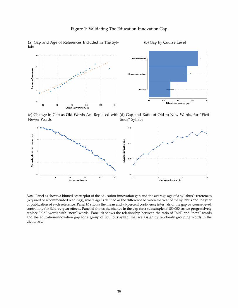
Figure 1: Validating The Education-Innovation Gap
(a) Gap and Age of References Included in The Syl-labi
(b) Gap by Course Level
(c) Change in Gap as Old Words Are Replaced withNewer Words
(d) Gap and Ratio of Old to New Words, for “Ficti-tious” Syllabi
Note: Panel a) shows a binned scatterplot of the education-innovation gap and the average age of a syllabus’s references(required or recommended readings), where age is defined as the difference between the year of the syllabus and the yearof publication of each reference. Panel b) shows the mean and 95-percent confidence intervals of the gap by course level,controlling for field-by-year effects. Panel c) shows the change in the gap for a subsample of 100,000, as we progressivelyreplace “old” words with “new” words. Panel d) shows the relationship between the ratio of “old” and “new” wordsand the education-innovation gap for a group of fictitious syllabi that we assign by randomly grouping words in thedictionary.
35

Figure 2: The Education-Innovation Gap and School Characteristics
Notes: Point estimates and 95-percent confidence intervals of coefficient β in equation (2), i.e., the slope of the relationshipbetween each reported variable and the education-innovation gap controlling for field-by course level-by-year fixedeffects. Each coefficient is estimated from a separate regression, with the exception of selectivity tiers (Ivy Plus/Elite,Highly Selective, Selective) which are jointly estimated. Endowment, expenditure, and share minority information refersto the year 2018 and is taken from IPEDS. Estimates are obtained pooling syllabi data for the years 1998 to 2018. Standarderrors are clustered at the school level.
36

Figure 3: Event Study: The Education-Innovation Gap when The Course Instructor Changes
Notes: Estimates and confidence intervals of the parameters δk in equation (2), representing an event study of theeducation-innovation gap around an instructor change episode and controlling for course and field-by-year effects. Ob-servations are at the course-by-year level; we focus on courses with at most two episodes of instructor changes. toStandard errors clustered at the course level.
37

Figure 4: Gap by Job Titles
Notes: Mean education-innovation gap by job title, along with 95-percent confidence intervals. Means are obtained asOLS coefficients from a regression of the gap on indicators for the job title of the instructor, as well as field-by-courselevel-by-year fixed effects. Estimates are obtained pooling data for multiple years. Standard errors are clustered at theschool level.
38

Figure 5: Instructors’ Research Productivity, Funding, and Fit with The Course The Education-Innovation Gap
(a) Publications, Last 5 Years (b) Citations, Last 5 Years
(c) Total #Grants (d) Fit Between Course Topic and Instructor’s Re-search
Notes: Binned scatterplot of the gap (vertical axis) and measures of research productivity, funding, and fit between thecourse topic and the research of the instructor. These measures are the number of publications in the last 5 years (panela); the number of citations in the last 5 years (panel b); the total number of NSF and NIH grants ever received (panel c);and the fit between the instructor’s research agenda and the course content, calculated as the cosine similarity betweenthe instructor’s publications and the syllabus of the course with the lowest gap among all courses on a given topic (forexample, Advanced Microeconomics) across schools in each year (panel d). All graphs control for field fixed effects.
39

Figure 6: The Education-Innovation Gap and Alternative Measures of Novelty: Binned Scatterplots
(a) Soft-skills intensity (b) Share of new knowledge
(c) Tail measure (d) Gap with patents
Notes: Binned scatterplots of the education-innovation gap and four alternative measures of novelty of each syllabus: ameasure of soft skills intensity, defined as the share of words in the assignment portion of a syllabus which refer to softskills (panel a); a measure of new knowledge, defined as the share of all new words contained by each syllabus (wherenew words are knowledge words that are (a) in the top 5 percent of the word frequency among articles published betweent−3 and t−1, or (b) used in articles published between t−3 and t−1 but not in those published between t−15 and t−13,panel b); a “tail measure,” calculated for each syllabus by (a) randomly selecting 100 subsamples containing 20 percent ofthe syllabus’s words, (b) calculating the gap for each subsample, and (c) selecting the 5th percentile of the correspondingdistribution (panel c); and the education-innovation gap calculated using the text of all patents as a benchmark, insteadof academic articles (panel d).
40

Table 1: Summary Statistics: Courses, Instructors, and Schools
Panel (a): Syllabus (Course) Characteristics
count mean std 25% 50% 75%
# Words 1,706,319 2226 1987 1068 1778 2796# Knowledge words 1,706,319 1011 1112 349 656 1236# Unique knowledge word 1,706,319 420 327 203 330 535Soft skills 1,703,863 33.4 22.9 14.0 30.5 50.0STEM 1,706,319 0.307 0.461 0 0 1Business 1,706,319 0.109 0.312 0 0 0Humanities 1,706,319 0.296 0.456 0 0 1Social science 1,706,319 0.257 0.437 0 0 0Basic 1,706,319 0.393 0.488 0 0 1Advanced 1,706,319 0.275 0.446 0 0 1Graduate 1,706,319 0.332 0.471 0 0 1
Panel (b): Instructor (Professor) Research Productivity
count mean std 25% 50% 75%
Ever Published? 727,165 0.36 0.48 0 0 1# Publications per year 262,344 1.64 2.06 1 1 1.70# Publications, last 5 years 262,344 6.47 15.22 0 1 6# Citations per year 262,344 35.34 108.23 0 4 26.94# Citations, last 5 years 262,344 175.37 840.61 0 0 61Ever Grant? 727,165 0.13 0.34 0 0 0# Grants 97,618 13.91 25.37 3 6 14Grant amount ($1,000) 97.62 5,332 21,100 489.89 1,621 4,672Salary ($) 63,632 80,388 62,364 34,798 73,027 110,831
Panel (c): Students’ Characteristics and Outcomes at University Level
count mean std 25% 50% 75%
Median parental income ($1,000) 767 97,917 31,054 78,000 93,500 109,900Share parents w/income in top 1% 767 0.030 0.041 0.006 0.013 0.033Share minority students 760 0.221 0.166 0.116 0.166 0.267Graduation rates (2012–13 cohort) 758 0.614 0.188 0.473 0.616 0.765Income (2003–04, 2004–05 cohorts) 762 45,035 10,235 38,200 43,300 49,800Intergenerational mobility 767 0.294 0.138 0.182 0.280 0.375Admission rate 715 0.642 0.218 0.533 0.683 0.800SAT score 684 1104.4 130.5 1011.5 1079.5 1182.0
Note: Summary statistics of main variables.
41

Table 2: Patterns of Sample Selection: Share of Syllabi Included in the Sample andInstitution-Level Characteristics
Panel (a): Share and ∆ Share, By School Tier
Share in OSP ∆Share in OSP, 2010-13
Corr. SE Corr. SEln Expenditure on instruction (2013) 0.002 (0.005) 0.015 (0.010)ln Endowment per capita (2000) -0.001 (0.002) -0.001 (0.002)ln Sticker price (2013) 0.003 (0.007) 0.007 (0.010)ln Avg faculty salary (2013) 0.016 (0.020) 0.049 (0.024)ln Enrollment (2013) 0.018 (0.009) 0.019 (0.011)Share Black students (2000) -0.030 (0.038) 0.035 (0.060)Share Hispanic students (2000) 0.171 (0.145) 0.161 (0.115)Share Asian students (2000) 0.186 (0.214) 0.324 (0.239)Share grad in Arts & Humanities (2000) 0.159 (0.168) 0.189 (0.179)Share grad in STEM (2000) -0.001 (0.028) 0.064 (0.056)Share grad in Social Sciences (2000) 0.014 (0.024) 0.104 (0.056)Share grad in Business (2000) 0.037 (0.065) 0.116 (0.065)F-stat 1.015 (.) 1.376 (.)
Panel (b): Share and ∆ Share, Correlation w/ School Characteristics
Share in OSP ∆Share in OSP, 2010-13
Mean SE Mean SEIvy Plus/Elite 0.009 (0.003) 0.022 (0.009)Highly Selective 0.004 (0.003) 0.006 (0.004)Selective Private 0.034 (0.026) 0.001 (0.029)Selective Public 0.045 (0.019) 0.009 (0.029)F-stat 4.076 (.) 1.806 (.)
Note: The top panel shows OLS coefficients (“means”) and robust standard errors (“SE”) of univariateregressions of each listed dependent variable on the corresponding independent variable. The bottompanel shows OLS coefficients (“means”) and syllabus-clustered standard errors (“SE”) of a regressionof each dependent variable on indicators for school tiers. The dependent variables are the school-levelshare of syllabi contained in the OSP sample in 2018 (columns 1-2) and the change in this share between2008 and 2018 columns (3-4). The F-statistics refer to multivariate regressions that include all the listedindependent variables, and test for the joint significance of these variables.
42

Table 3: Decomposing the Gap: Contribution of Institutions, Years, Fields, Courses, and Instructors
Variable Partial R2
Year 0.169 0.180Field 0.039 0.056School 0.021 0.028Course level . 0.008Course 0.330 .Instructor 0.248 0.346Total 0.161 0.124
Note: The table shows a decomposition of the R2 of a regression of the education-innovation gap on all sets oflisted fixed effects into the contribution of each set of fixed effects. This is done using the Shapley-Owen decompo-sition method, which calculates the partial R2 of each set of variables j as R2
j =∑k 6=j
R2−R2(−j)K!/j!(K−j−1)!
where R2(−j)is the R2 of a regression that excludes variables j. Column 1 inlcudes course fixed effects; column 2 only in-cludes course level fixed effects. We use adjusted R2 in lieu of R2 to account for the large number of fixed effects.
43

Tabl
e4:
The
Educ
atio
n-In
nova
tion
Gap
Whe
nth
eIn
stru
ctor
Cha
nges
:Eve
ntSt
udy
All
Fiel
dsBu
sine
ssH
uman
itie
sST
EMSo
cial
Scie
nce
Basi
cA
dvan
ced
Gra
duat
eIn
stru
ctor
chan
ge(1
)(2
)(3
)(4
)(5
)(6
)(7
)(8
)
Aft
erch
ange
-0.0
956*
**-0
.099
3-0
.121
1**
-0.0
958*
*-0
.022
5-0
.080
2*-0
.074
3*-0
.114
5***
(0.0
244)
(0.0
698)
(0.0
481)
(0.0
438)
(0.0
418)
(0.0
456)
(0.0
450)
(0.0
375)
N(C
ours
ex
year
)37
9459
3559
897
380
1340
7094
574
1254
6911
2174
1377
55#
Cou
rses
1263
5211
558
3320
940
129
3158
943
533
3538
646
226
Cou
rse
FEYe
sYe
sYe
sYe
sYe
sYe
sYe
sYe
sFi
eld
xYe
arFE
Yes
Yes
Yes
Yes
Yes
Yes
Yes
Yes
Not
e:O
LSes
tim
ates
,one
obse
rvat
ion
isa
cour
se.T
hede
pend
entv
aria
ble
isth
eed
ucat
ion-
inno
vati
onga
p.Th
eva
riab
leA
fterc
hang
eis
anin
dica
tor
for
year
sfo
llow
ing
anin
stru
ctor
chan
ge,f
orco
urse
sw
ith
only
one
inst
ruct
oran
dat
mos
ttw
oin
stru
ctor
chan
ges
over
the
obse
rved
tim
epe
riod
.All
spec
ifica
tion
sco
ntro
lfor
cour
sean
dfie
ld-b
y-ye
arfix
edef
fect
s.St
anda
rder
rors
inpa
rent
hese
sar
ecl
uste
red
atth
eco
urse
leve
l.∗≤
0.1
,∗∗≤
0.05
,∗∗∗≤
0.01
.
44

Tabl
e5:
The
Educ
atio
n-In
nova
tion
Gap
and
Inst
ruct
orR
esea
rch
Prod
ucti
vity
:Pub
licat
ions
and
Cit
atio
ns
All
Fiel
dsBu
sine
ssH
uman
itie
sST
EMSo
cial
Scie
nce
Basi
cA
dvan
ced
Gra
duat
ePa
nela
):#p
ubli
cati
ons
(1)
(2)
(3)
(4)
(5)
(6)
(7)
(8)
1stq
uart
ile-0
.026
00.
0527
-0.0
834*
*0.
0432
-0.0
692*
*-0
.014
4-0
.025
3-0
.038
0(0
.018
6)(0
.047
9)(0
.033
8)(0
.039
3)(0
.029
3)(0
.031
1)(0
.033
3)(0
.031
8)
2nd
quar
tile
0.00
760.
0300
0.07
89-0
.048
80.
0012
0.03
06-0
.002
3(0
.032
1)(0
.074
2)(0
.054
7)(0
.042
8)(0
.057
4)(0
.059
0)(0
.050
3)
3rd
quar
tile
-0.0
102
0.07
88-0
.048
00.
0983
-0.1
085*
*0.
0274
0.00
05-0
.051
3(0
.031
1)(0
.072
9)(0
.070
7)(0
.059
8)(0
.046
1)(0
.058
8)(0
.055
5)(0
.047
9)
4th
quar
tile
-0.1
086*
**0.
0475
-0.1
065
-0.0
637
-0.1
773*
**-0
.033
7-0
.094
7-0
.173
1***
(0.0
386)
(0.0
912)
(0.0
811)
(0.0
735)
(0.0
626)
(0.0
758)
(0.0
715)
(0.0
571)
Pane
lb):
#cit
atio
ns(1
)(2
)(3
)(4
)(5
)(6
)(7
)(8
)
1stq
uart
ile0.
0305
0.00
260.
0478
0.13
08**
*-0
.052
20.
0465
0.06
69-0
.009
2(0
.025
9)(0
.067
6)(0
.065
0)(0
.047
3)(0
.036
3)(0
.044
0)(0
.046
8)(0
.043
3)
2nd
quar
tile
0.01
950.
0135
-0.0
315
0.11
16**
-0.0
424
0.02
820.
0128
0.01
87(0
.029
2)(0
.068
9)(0
.068
2)(0
.053
9)(0
.043
4)(0
.052
1)(0
.052
3)(0
.047
2)
3rd
quar
tile
-0.0
802*
*-0
.025
4-0
.069
8-0
.061
1-0
.117
1**
0.00
81-0
.111
5*-0
.124
9**
(0.0
334)
(0.0
788)
(0.0
809)
(0.0
621)
(0.0
494)
(0.0
638)
(0.0
619)
(0.0
497)
4th
quar
tile
-0.0
624
0.07
74-0
.095
4-0
.011
9-0
.125
7*-0
.014
4-0
.034
5-0
.134
5**
(0.0
426)
(0.0
963)
(0.1
083)
(0.0
768)
(0.0
662)
(0.0
826)
(0.0
796)
(0.0
625)
N(C
ours
ex
year
)57
1449
5976
814
4945
1688
6614
9578
2073
6016
8992
1948
29#
Cou
rses
1515
8714
889
3975
644
848
3887
255
041
4293
653
539
Cou
rse
FEYe
sYe
sYe
sYe
sYe
sYe
sYe
sYe
sFi
eld
xYe
arFE
Yes
Yes
Yes
Yes
Yes
Yes
Yes
Yes
Not
e:O
LSes
tim
ates
,one
obse
rvat
ion
isa
cour
se.
The
depe
nden
tva
riab
leis
the
educ
atio
n-in
nova
tion
gap;
the
inde
pend
ent
vari
able
sar
ein
dica
tors
for
quar
tile
sof
the
num
ber
ofpu
blic
atio
ns(p
anel
(a))
and
cita
tion
s(p
anel
(b))
ofa
cour
se’s
inst
ruct
ors
inth
epr
evio
usfiv
eye
ars.
The
omit
ted
cate
gory
are
cour
ses
wit
hin
stru
ctor
sw
ith
nopu
blic
atio
nsor
cita
tion
s.Fo
rco
urse
sw
ith
mor
eth
anon
ein
stru
ctor
,we
cons
ider
the
mea
nnu
mbe
rof
publ
icat
ions
and
cita
tion
sac
ross
alli
nstr
ucto
rs.
All
spec
ifica
tion
sco
ntro
lfor
cour
sean
dfie
ld-b
y-ye
arfix
edef
fect
s.St
anda
rder
rors
inpa
rent
hese
sar
ecl
uste
red
atth
eco
urse
leve
l.∗≤
0.1
,∗∗≤
0.05
,∗∗∗≤
0.01
.
45

Tabl
e6:
The
Educ
atio
n-In
nova
tion
Gap
,Ins
truc
tor
Cha
nges
,and
FitB
etw
een
Inst
ruct
ors’
Res
earc
han
dC
ours
eC
onte
nt
All
Fiel
dsBu
sine
ssH
uman
itie
sST
EMSo
cial
Scie
nce
Basi
cA
dvan
ced
Gra
duat
e(1
)(2
)(3
)(4
)(5
)(6
)(7
)(8
)
Fitw
/top
cour
se(s
d)-0
.087
7**
0.14
800.
0017
-0.0
836
-0.0
849
-0.0
637
-0.1
428*
-0.0
611
(0.0
398)
(0.1
001)
(0.1
723)
(0.0
608)
(0.0
656)
(0.0
832)
(0.0
790)
(0.0
558)
N(C
ours
ex
year
)54
591
3199
2218
3311
912
587
1674
316
224
2113
9#
Cou
rses
1707
710
1176
110
267
3909
5208
4833
6883
Cou
rse
FEYe
sYe
sYe
sYe
sYe
sYe
sYe
sYe
sFi
eld
xYe
arFE
Yes
Yes
Yes
Yes
Yes
Yes
Yes
Yes
Not
e:O
LSes
tim
ates
,one
obse
rvat
ion
isa
cour
se.
The
depe
nden
tva
riab
leis
the
educ
atio
n-in
nova
tion
gap.
The
vari
able
Fit
w/t
opco
urse
isa
mea
sure
offit
betw
een
the
inst
ruct
or’s
rese
arch
and
the
cont
ento
fthe
cour
se,d
efine
das
the
cosi
nesi
mila
rity
betw
een
the
inst
ruct
or’s
rese
arch
inth
epr
evio
us5
year
san
dth
eco
nten
toft
heco
urse
wit
hth
esm
alle
sted
ucat
ion-
inno
vati
onac
ross
scho
ols
inth
esa
me
topi
c.A
llsp
ecifi
cati
ons
cont
rolf
orco
urse
and
field
-by-
year
fixed
effe
cts.
Stan
dard
erro
rsin
pare
nthe
ses
are
clus
tere
dat
the
cour
sele
vel.∗≤
0.1
,∗∗≤
0.05
,∗∗∗≤
0.01
.
46

Tabl
e7:
The
Educ
atio
n-In
nova
tion
Gap
and
Inst
ruct
orR
esea
rch
Res
ourc
es:G
rant
num
bers
and
amou
nt
All
Fiel
dsBu
sine
ssH
uman
itie
sST
EMSo
cial
Scie
nce
Basi
cA
dvan
ced
Gra
duat
e(1
)(2
)(3
)(4
)(5
)(6
)(7
)(8
)
Atl
east
one
gran
t-0
.054
4**
-0.0
244
-0.0
666
-0.0
639
-0.0
785*
*-0
.043
6-0
.061
4-0
.060
1(0
.022
0)(0
.066
4)(0
.046
6)(0
.039
4)(0
.037
5)(0
.036
0)(0
.041
3)(0
.037
2)
N(C
ours
ex
year
)58
1995
5976
814
4945
1688
6614
9578
2101
2117
1867
1997
35#
Cou
rses
1538
0914
889
3975
644
848
3887
255
594
4347
454
663
Cou
rse
FEYe
sYe
sYe
sYe
sYe
sYe
sYe
sYe
sFi
eld
xYe
arFE
Yes
Yes
Yes
Yes
Yes
Yes
Yes
Yes
Not
e:O
LSes
tim
ates
,one
obse
rvat
ion
isa
cour
se.
The
depe
nden
tva
riab
leis
the
educ
atio
n-in
nova
tion
gap.
The
vari
able
At
leas
ton
egr
ant
equa
lson
eif
the
cour
se’s
inst
ruct
or(o
rat
leas
tone
ofth
eco
urse
’sin
stru
ctor
sin
case
ofm
ulti
ple
inst
ruct
ors)
has
rece
ived
atle
asto
neN
SFor
NIH
gran
t.A
llsp
ecifi
cati
ons
cont
rolf
orco
urse
and
field
-by-
year
fixed
effe
cts.
Stan
dard
erro
rsin
pare
nthe
ses
are
clus
tere
dat
the
cour
sele
vel.∗≤
0.1
,∗∗≤
0.05
,∗∗∗≤
0.01
.
47

Table 8: The Education-Innovation Gap and Instructor Salaries
(1) (2) (3) (4) (5)
ln(salary) -0.051*** -0.050*** -0.029(0.019) (0.019) (0.031)
Field x level x year FE Yes Yes Yes
School FE No Yes Yes
Job title FE No No Yes
Observations 139516 139446 99669
Note: OLS estimates. The dependent variable is the education-innovation gap. The variable ln(salary) is the natural loga-rithm of total instructor pay, for a subset of public-sector instructors. All specifications control forfield-by-course level-byyear fixed effects; columns 2 and 5 controls for age fixed effects, columns 3 and 5 control for school fixed effects, andcolumns 4 and 5 control for job title fixed effects. Age is defined as the difference between the year of the syllabus andthe year of first publication of the instructor. Standard errors in parentheses are clustered at the course level. ∗ ≤ 0.1,∗∗ ≤ 0.05, ∗∗∗ ≤ 0.01.
48

Tabl
e9:
The
Educ
atio
n-In
nova
tion
Gap
and
Stud
entO
utco
mes
Inco
me
(Col
lege
Scor
ecar
d)In
com
e(C
hett
yet
al.,
2019
)
Gra
dra
teM
ean
P y≤
33pc
tile
Med
ian
Mea
nP(
top
20%
)P(
top
10%
)P(
top
5%)
P(to
p20
%|P
y≤
20pc
tile
)Pa
nel(
a):n
oco
ntro
ls(1
)(2
)(3
)(4
)(5
)(6
)(7
)(8
)(9
)
Gap
(sd)
-0.0
513*
**-0
.055
5***
-0.0
645*
**-0
.051
2***
-0.0
722*
**-0
.033
3***
-0.0
265*
**-0
.018
7***
-0.0
293*
**(0
.006
8)(0
.010
4)(0
.010
6)(0
.008
8)(0
.012
4)(0
.005
7)(0
.004
6)(0
.003
6)(0
.005
3)
Mea
nde
p.va
r.0.
5692
0.36
940.
2082
0.11
430.
2945
N15
683
3793
3566
3793
763
763
763
763
763
#sc
hool
s76
176
073
476
0
Pane
l(b)
:wit
hco
ntro
ls(1
)(2
)(3
)(4
)(5
)(6
)(7
)(8
)(9
)
Gap
(sd)
-0.0
073*
*-0
.006
7-0
.008
3*-0
.009
0**
-0.0
137*
**-0
.008
4***
-0.0
053*
*-0
.003
1**
-0.0
047*
(0.0
030)
(0.0
041)
(0.0
050)
(0.0
045)
(0.0
048)
(0.0
025)
(0.0
021)
(0.0
015)
(0.0
028)
Mea
nde
p.va
r.0.
5816
10.8
281
10.7
605
10.7
096
0.37
100.
2100
0.11
590.
2957
N11
471
1996
1843
1996
718
718
718
718
718
#sc
hool
s73
372
770
172
7
Not
e:O
LSes
tim
ates
ofth
eco
effic
ientδ
ineq
uati
on(4
).Th
eva
riab
leG
ap(s
d)is
asc
hool
-lev
eled
ucat
ion-
inno
vati
onga
p(e
stim
ated
asθ s
(i)
ineq
uati
on(3
)),s
tand
ard-
ized
toha
vem
ean
zero
and
vari
ance
one.
The
depe
nden
tvar
iabl
ear
egr
adua
tion
rate
s(f
rom
IPED
S,ye
ars
1998
-201
8,co
lum
n1)
;the
log
ofm
ean
stud
enti
ncom
esfr
omth
eC
olle
geSc
orec
ard,
for
alls
tude
nts
(col
umn
2)an
dfo
rst
uden
tsw
ith
pare
ntal
inco
me
inth
ebo
ttom
terc
ile(c
olum
n3)
;the
log
ofm
edia
nin
com
efr
omth
eC
olle
geSc
orec
ard
(col
umn
4);t
helo
gof
mea
nin
com
efo
rst
uden
tsw
hogr
adua
ted
betw
een
2002
and
2004
(fro
mC
hett
yet
al.(
2019
),co
lum
n5)
;the
prob
abili
tyth
atst
uden
tsha
vein
com
esin
the
top
20,1
0,an
d5
perc
ent
ofth
ena
tion
aldi
stri
buti
on(f
rom
Che
tty
etal
.(20
19),
colu
mns
6-8)
;and
the
prob
abili
tyth
atst
uden
tsw
ith
pare
ntal
in-
com
ein
the
bott
omqu
inti
lere
ach
the
top
quin
tile
duri
ngad
ulth
ood
(col
umn
9).C
olum
ns1-
4in
pane
lsa
and
bco
ntro
lfor
year
effe
cts.
All
colu
mns
inpa
nelb
cont
rol
for
cont
rol(
priv
ate
orpu
blic
),se
lect
ivit
yti
ers,
and
anin
tera
ctio
nbe
twee
nse
lect
ivit
yti
ers
and
anin
dica
tor
for
R1
inst
itut
ions
acco
rdin
gto
the
Car
negi
ecl
assi
ficat
ion;
stud
ent-
to-f
acul
tyra
tio
and
the
shar
eof
ladd
erfa
cult
y;to
tale
xpen
ditu
re,r
esea
rch
expe
ndit
ure,
inst
ruct
iona
lexp
endi
ture
,and
sala
ryin
stru
ctio
nale
xpen
ditu
repe
rst
uden
t;th
esh
are
ofun
derg
radu
ate
and
grad
uate
enro
llmen
tand
the
shar
eof
whi
tean
dm
inor
ity
stud
ents
;an
indi
cato
rfo
rin
stit
utio
nsw
ith
adm
issi
onsh
are
equa
lto
100,
med
ian
SAT
and
AC
Tsc
ores
ofad
mit
ted
stud
ents
in20
06,a
ndin
dica
tors
for
scho
ols
not
usin
gei
ther
SAT
orA
CT
inad
mis
sion
;the
shar
eof
stud
ents
wit
hm
ajor
sin
Art
san
dH
uman
itie
s,Bu
sine
ss,H
ealt
h,Pu
blic
and
Soci
alSe
rvic
e,So
cial
Scie
nces
,STE
M,a
ndm
ulti
-dis
cipl
inar
yfie
lds;
and
the
natu
rall
ogar
ithm
ofpa
rent
alin
com
e.Bo
otst
rapp
edst
anda
rder
rors
inpa
rent
hese
sar
ecl
uste
red
atth
esc
hool
leve
l.∗≤
0.1
,∗∗≤
0.05
,∗∗∗≤
0.01
.
49

AppendixFor online publication only
A1

Additional Tables and Figures
A2

Figure AI: Distribution of Instructor Job Titles and Average Salary
(a) Job Title Distribution
(b) Average Salary and 95-percent Confidence Intervals
Note: Panel (a): share of syllabi instructors by job title. Panel (b): Average salary and 95-percent confidence intervals by jobtitle. The same is restricted to 35,178 instructors in public institutions for whom title information is available.
A3

Figure AII: Number of Syllabi In The Sample, By Year
Note: Number of syllabi included in final sample, by year.
A4

Figure AIII: Macro-Field Coverage, Course Catalogs and Syllabi Sample
(a) Course Catalog (b) Syllabi Sample
Note: Composition across macro fields, for all courses included in a sample of school catalogs (panel (a)) and for coursesincluded in the syllabi sample (panel (b)).
Figure AIV: Course Level Coverage, Course Catalogs and Syllabi Sample
(a) Course Catalog (b) Syllabi Sample
Note: Composition across course levels, for all courses included in a sample of school catalogs (panel (a)) and for coursesincluded in the syllabi sample (panel (b)).
A5

Figure AV: Share of Catalog Courses in the Syllabi Sample
Note: Share of courses from full course catalogs whose syllabi are included in the syllabi sample.
A6

Figure AVI: Education-Innovation Gap: Variation
Notes: Distribution of the gap. The solid line shows the raw data; the other series show the residuals of regressions as weprogressively control for additional sets of fixed effects.
A7

Figu
reA
VII
:Sch
oolC
hara
cter
isti
csan
dA
lter
nati
veM
easu
res
ofC
ours
eN
ovel
ty
(a)S
ofts
kills
inte
nsit
y(b
)Sha
reof
old
know
ledg
e
(c)T
ailm
easu
re(d
)Gap
w/p
aten
ts
Not
es:P
oint
esti
mat
esan
d95
-per
cent
confi
denc
ein
terv
als
ofco
effic
ientβ
ineq
uati
on(2
),us
ing
alte
rnat
ive
mea
sure
sof
cour
seno
velt
y:a
mea
sure
ofso
ftsk
ills
inte
nsit
y,de
fined
asth
esh
are
ofw
ords
inth
eas
sign
men
tpor
tion
ofa
sylla
bus
whi
chre
fer
toso
ftsk
ills
(pan
eld)
.am
easu
reof
new
know
ledg
e,de
fined
asth
esh
are
ofal
lnew
wor
dsco
ntai
ned
byea
chsy
llabu
s(w
here
new
wor
dsar
ekn
owle
dge
wor
dsth
atar
e(a
)in
the
top
5pe
rcen
toft
hew
ord
freq
uenc
yam
ong
arti
cles
publ
ishe
dbe
twee
nt−
3an
dt−
1,o
r(b
)us
edin
arti
cles
publ
ishe
dbe
twee
nt−
3an
dt−
1bu
tnot
inth
ose
publ
ishe
dbe
twee
nt−
15
andt−
13
,pan
elb)
;a“t
ailm
easu
re,”
calc
ulat
edfo
rea
chsy
llabu
sby
(a)r
ando
mly
sele
ctin
g10
0su
bsam
ples
cont
aini
ng20
perc
ento
fthe
sylla
bus’
sw
ords
,(b)
calc
ulat
ing
the
gap
for
each
subs
ampl
e,an
d(c
)sel
ecti
ngth
e5t
hpe
rcen
tile
ofth
eco
rres
pond
ing
dist
ribu
tion
(pan
elc)
;an
dth
eed
ucat
ion-
inno
vati
onga
pca
lcul
ated
usin
gth
ete
xtof
all
pate
nts
asa
benc
hmar
k,in
stea
dof
acad
emic
arti
cles
(pan
eld)
.Ea
chco
effic
ient
ises
tim
ated
from
ase
para
tere
gres
sion
,wit
hth
eex
cept
ion
ofse
lect
ivit
yti
ers
(Ivy
Plus
/Elit
e,H
ighl
ySe
lect
ive,
Sele
ctiv
e)w
hich
are
join
tly
esti
mat
ed.E
ndow
men
t,ex
pend
itur
e,an
dsh
are
min
orit
yin
form
atio
nre
fers
toth
eye
ar20
18an
dis
take
nfr
omIP
EDS.
Esti
mat
esar
eob
tain
edpo
olin
gsy
llabi
data
for
the
year
s19
98to
2018
.Sta
ndar
der
rors
are
clus
tere
dat
the
scho
olle
vel.
A8

Figu
reA
VII
I:In
stru
ctor
Prod
ucti
vity
(#Pu
blic
atio
ns)a
ndA
lter
nati
veM
easu
res
ofC
ours
eN
ovel
ty
(a)S
ofts
kills
inte
nsit
y(b
)Sha
reof
new
know
ledg
e
(c)T
ailm
easu
re(d
)Gap
w/p
aten
ts
Not
es:
Binn
edsc
atte
rplo
tsof
am
easu
reof
inst
ruct
orpr
oduc
tivi
ty(t
henu
mbe
rof
cita
tion
sin
the
prio
r5
year
s)an
dfo
ural
tern
ativ
em
easu
res
ofco
urse
nove
lty:
am
easu
reof
soft
skill
sin
tens
ity,
defin
edas
the
shar
eof
wor
dsin
the
assi
gnm
entp
orti
onof
asy
llabu
sw
hich
refe
rto
soft
skill
s(p
anel
a),a
mea
sure
ofne
wkn
owle
dge,
defin
edas
the
shar
eof
alln
eww
ords
cont
aine
dby
each
sylla
bus
(whe
rene
ww
ords
are
know
ledg
ew
ords
that
are
(a)i
nth
eto
p5
perc
ento
fthe
wor
dfr
eque
ncy
amon
gar
ticl
espu
blis
hed
betw
eent−
3an
dt−
1,o
r(b
)use
din
arti
cles
publ
ishe
dbe
twee
nt−
3an
dt−
1bu
tnot
inth
ose
publ
ishe
dbe
twee
nt−
15
andt−
13
,pan
elb)
;a“t
ailm
easu
re,”
calc
ulat
edfo
rea
chsy
llabu
sby
(a)
rand
omly
sele
ctin
g10
0su
bsam
ples
cont
aini
ng20
perc
ent
ofth
esy
llabu
s’s
wor
ds,(
b)ca
lcul
atin
gth
ega
pfo
rea
chsu
bsam
ple,
and
(c)s
elec
ting
the
5th
perc
enti
leof
the
corr
espo
ndin
gdi
stri
buti
on(p
anel
c);a
ndth
eed
ucat
ion-
inno
vati
onga
pca
lcul
ated
usin
gth
ete
xtof
allp
aten
tsas
abe
nchm
ark,
inst
ead
ofac
adem
icar
ticl
es(p
anel
d).R
elat
ions
hips
are
plot
ted
cont
rolli
ngfo
rfie
ldef
fect
s.
A9

Figure AIX: Distribution of School-Level Gap
Note: Distribution of φs, the school-level component of the gap, corresponding to θs(i) in equation (3).
A10

Table AI: Categorization of Course (Macro-)Fields
Macro-field Fields
Business Business, Accounting, Marketing
Humanities English Literature, Media / CommunicationsPhilosophy, Theology, Criminal JusticeLibrary Science, Classics, Women’s StudiesJournalism, Religion, Sign LanguageMusic, Theatre Arts, Fine Arts, HistoryFilm and Photography, Dance, Anthropology
STEM Mathematics, Computer Science, BiologyEngineering, Chemistry, PhysicsArchitecture, Agriculture, Earth SciencesBasic Computer Skills, Astronomy, TransportationAtmospheric Sciences
Social Sciences Psychology, Political Science, EconomicsLaw, Social Work, GeographyLinguistics, Sociology Education
Vocational Fitness and Leisure, Basic SkillsMechanic / Repair Tech, CosmetologyCulinary Arts, Health Technician, Public Safety
Note: Mapping between the “macro-fields” used in our analysis and syllabi’s “fields”as reported in the OSP dataset.
A11

Table AII: List of Institutions in the Catalog Data
Institution Institution
Aiken Technical College Minnesota State University MoorheadAlabama Agricultural and Mechanical University Mississippi CollegeAlabama State University Mississippi Community College BoardAlexandria Technical and Community College Missouri State UniversityArkansas Tech University Mitchell Technical InstituteAsnuntuck Community College Montgomery CollegeBay Path University Morehead State UniversityBenedictine University Mountain Empire Community CollegeBentley University Mountwest Community and Technical CollegeBluegrass Community and Technical College Mt. San Antonio CollegeBriar Cliff University New Mexico State University AlamogordoBrown University Niagara UniversityBryan College Nichols CollegeCalifornia Baptist University North Carolina State UniversityCalifornia Lutheran University North Florida Community CollegeCalifornia Polytechnic State University Northwest Arkansas Community CollegeCamden County College Oakwood UniversityCampbell University Oral Roberts UniversityCardinal Stritch University Orangeburg-Calhoun Technical CollegeCarlow University Oregon State UniversityCatawba College Oxnard CollegeCecil College Penn State New KensingtonCedarville University Plymouth State UniversityCenter for Creative Studies Princeton UniversityCerritos College Richland Community CollegeCoe College Robeson Community CollegeCollege of Alameda Rocky Mountain CollegeCollege of Southern Nevada SUNY College at Old WestburyCollege of the Siskiyous SUNY OneontaColumbia University SUNY OrangeConcordia University Texas San Diego Mesa CollegeCopiah-Lincoln Community College San Diego Miramar CollegeCounty College of Morris San Diego State UniversityDartmouth College South Arkansas Community CollegeDaytona State College Southern University at New OrleansDominican University Spring Arbor UniversityDuke University Spring Hill CollegeEastern Nazarene College Stanford UniversityENMU-Ruidoso Branch Community College State University of New York at PotsdamElmhurst College Suffolk County Community CollegeFlorida Gulf Coast University Texas Lutheran UniversityFlorida Institute of Technology The University of Texas Rio Grande ValleyFresno Pacific University Three Rivers Community CollegeFrostburg State University Trevecca Nazarene University
(Continued)
A12

Table AII. Continued
Institution Institution
George Mason University Trocaire CollegeGeorgia State University University of AkronGlendale Community College University of Central OklahomaGrays Harbor College University of ChicagoGreen River Community College University of Colorado DenverGrossmont College University of EvansvilleHelena College University of Montana University of LouisvilleHerkimer County Community College University of Maine at Presque IsleHibbing Community College University of Missouri-St. LouisHood College University of MontanaHudson County Community College University of North Carolina at Chapel HillIndiana University Northwest University of North DakotaIowa Central Community College University of North TexasJackson State Community College University of Notre DameJefferson State Community College University of PennsylvaniaKankakee Community College University of PittsburghKellogg Community College University of South Carolina AikenKettering University University of South Florida Sarasota-ManateeKeystone College University of Wisconsin-River FallsKing’s College - Pennsylvania Upper Iowa UniversityKutztown University Vanderbilt UniversityLake Forest College Virginia Highlands Community CollegeLas Positas College Wayne State CollegeLassen Community College Weber State UniversityLeeward Community College Webster UniversityLincoln University - Missouri Wenatchee Valley CollegeLong Beach City College Wentworth Institute of TechnologyLos Medanos College Wesleyan UniversityLouisiana State University in Shreveport Western Dakota Technical InstituteMacmurray College Western State Colorado UniversityMarian University - Indiana William Jewell CollegeMarian University - Wisconsin William Woods UniversityMarietta College Yale UniversityMartin Luther College Youngstown State UniversityMartin Methodist College Yuba CollegeMillsaps College
Note: List of schools for which we collected course catalog data.
A13

Tabl
eA
III:
Scho
olC
hara
cter
isti
csof
Scho
ols
Inan
dO
utof
Cat
alog
Dat
a
Mea
nfo
rIn
stit
utio
nsIn
the
Sam
ple
Mea
nfo
rIn
stit
utio
nsO
utof
the
Sam
ple
t-st
atis
tics
p-v
alue
s#
Inst
itut
ions
=15
8#
Inst
itut
ions
=1,
956
lnEx
pend
itur
eon
inst
ruct
ion
(201
3)8.
693
8.60
1-1
.725
0.08
5ln
Endo
wm
entp
erca
pita
(200
0)6.
857
6.48
3-1
.304
0.19
3ln
Stic
ker
pric
e(2
013)
9.19
79.
153
-0.5
200.
603
lnA
vgfa
cult
ysa
lary
(201
3)8.
890
8.85
0-1
.897
0.05
8ln
Enro
llmen
t(20
13)
8.70
88.
634
-0.6
850.
494
Shar
eBl
ack
stud
ents
(200
0)0.
109
0.11
20.
153
0.87
9Sh
are
His
pani
cst
uden
ts(2
000)
0.06
30.
065
0.18
30.
855
Shar
eal
ien
stud
ents
(200
0)0.
025
0.02
2-1
.030
0.30
3Sh
are
grad
inA
rts
&H
uman
itie
s(2
000)
7.58
17.
958
0.38
20.
703
Shar
egr
adin
STEM
(200
0)14
.861
14.0
50-0
.772
0.44
0Sh
are
grad
inSo
cial
Scie
nces
(200
0)21
.068
19.2
02-1
.342
0.18
0
Not
e:Ba
lanc
ete
stof
univ
ersi
ties
inan
dou
toft
heca
talo
gsa
mpl
e.
A14

Tabl
eA
IV:A
lter
nati
veM
easu
res
ofN
ovel
tyan
dSt
uden
tOut
com
es
Inco
me
(Col
lege
Scor
ecar
d)In
com
e(C
hett
yet
al.,
2019
)
Gra
dra
teM
ean
P y≤
33pc
tile
Med
ian
Mea
nP(
top
20%
)P(
top
10%
)P(
top
5%)
P(to
p20
%|P
y≤
20pc
tile
)(1
)(2
)(3
)(4
)(5
)(6
)(7
)(8
)(9
)Pa
nel(
a):S
hare
new
know
ledg
e,no
cont
rols
Gap
(sd)
0.04
24**
*0.
0594
***
0.06
78**
*0.
0499
***
0.07
55**
*0.
0338
***
0.03
03**
*0.
0226
***
0.03
10**
*(0
.008
1)(0
.010
3)(0
.012
1)(0
.010
1)(0
.013
7)(0
.006
6)(0
.005
3)(0
.004
0)(0
.006
2)
Mea
nde
p.va
r.0.
5692
0.36
940.
2082
0.11
430.
2945
N15
683
3793
3566
3793
763
763
763
763
763
#sc
hool
s76
176
073
476
0
Pane
l(b)
:Sha
rene
wkn
owle
dge,
wit
hco
ntro
ls
Gap
(sd)
0.00
400.
0034
0.00
270.
0018
0.01
09**
0.00
480.
0041
*0.
0032
*0.
0004
(0.0
036)
(0.0
049)
(0.0
057)
(0.0
051)
(0.0
045)
(0.0
032)
(0.0
021)
(0.0
017)
(0.0
032)
Mea
nde
p.va
r.0.
5816
10.8
281
10.7
605
10.7
096
0.37
100.
2100
0.11
590.
2957
N11
471
1996
1843
1996
718
718
718
718
718
#sc
hool
s73
372
770
172
7
Pane
l(c)
:Tai
lmea
sure
,no
cont
rols
Gap
(sd)
-0.0
503*
**-0
.064
3***
-0.0
714*
**-0
.058
0***
-0.0
882*
**-0
.039
3***
-0.0
336*
**-0
.024
5***
-0.0
385*
**(0
.009
0)(0
.010
5)(0
.011
9)(0
.010
1)(0
.012
5)(0
.005
6)(0
.005
0)(0
.003
6)(0
.005
6)
Mea
nde
p.va
r.0.
5692
0.36
940.
2082
0.11
430.
2945
N15
683
3793
3566
3793
763
763
763
763
763
#sc
hool
s76
176
073
476
0
Pane
l(d)
:Tai
lmea
sure
,wit
hco
ntro
ls
Gap
(sd)
-0.0
023
-0.0
123*
**-0
.016
6***
-0.0
137*
**-0
.019
4***
-0.0
113*
**-0
.008
9***
-0.0
057*
**-0
.012
1***
(0.0
034)
(0.0
043)
(0.0
047)
(0.0
049)
(0.0
048)
(0.0
027)
(0.0
023)
(0.0
016)
(0.0
030)
Mea
nde
p.va
r.0.
5816
10.8
281
10.7
605
10.7
096
0.37
100.
2100
0.11
590.
2957
N11
471
1996
1843
1996
718
718
718
718
718
#sc
hool
s73
372
770
172
7
Pane
l(e)
:Gap
w/p
aten
ts,n
oco
ntro
ls
Gap
(sd)
-0.0
232*
**-0
.032
3***
-0.0
434*
**-0
.028
2***
-0.0
404*
**-0
.014
4**
-0.0
140*
*-0
.012
0***
-0.0
146*
*(0
.006
8)(0
.011
6)(0
.012
2)(0
.009
9)(0
.013
8)(0
.006
7)(0
.005
9)(0
.004
2)(0
.006
4)
Mea
nde
p.va
r.0.
5692
0.36
940.
2082
0.11
430.
2945
N15
683
3793
3566
3793
763
763
763
763
763
#sc
hool
s76
176
073
476
0
(Con
tinu
ed)
A15

Tabl
eA
IV.C
onti
nued
Gra
dra
teM
ean
P y≤
33pc
tile
Med
ian
Mea
nP(
top
20%
)P(
top
10%
)P(
top
5%)
P(to
p20
%|P
y≤
20pc
tile
)
Pane
l(f)
:Gap
w/p
aten
ts,w
ith
cont
rols
Gap
(sd)
-0.0
049
-0.0
003
-0.0
023
-0.0
007
-0.0
039
0.00
04-0
.001
5-0
.002
3*-0
.001
4(0
.003
2)(0
.003
8)(0
.004
4)(0
.004
2)(0
.004
6)(0
.002
5)(0
.002
0)(0
.001
2)(0
.002
9)
Mea
nde
p.va
r.0.
5816
10.8
281
10.7
605
10.7
096
0.37
100.
2100
0.11
590.
2957
N11
471
1996
1843
1996
718
718
718
718
718
#sc
hool
s73
372
770
172
7
Pane
l(g)
:Sof
tski
lls
inte
nsit
y,no
cont
rols
Gap
(sd)
0.09
82**
*0.
0935
***
0.09
66**
*0.
0818
***
0.11
25**
*0.
0497
***
0.03
94**
*0.
0293
***
0.05
21**
*(0
.006
5)(0
.009
1)(0
.011
3)(0
.008
5)(0
.011
5)(0
.005
2)(0
.004
4)(0
.003
5)(0
.005
3)
Mea
nde
p.va
r.0.
5692
0.36
940.
2082
0.11
430.
2945
N15
683
3793
3566
3793
763
763
763
763
763
#sc
hool
s76
176
073
476
0
Pane
l(h)
:Sof
tski
lls
inte
nsit
y,w
ith
cont
rols
Gap
(sd)
0.01
16**
*0.
0172
***
0.00
960.
0209
***
0.01
25**
0.01
03**
*0.
0028
0.00
070.
0119
***
(0.0
034)
(0.0
052)
(0.0
068)
(0.0
058)
(0.0
057)
(0.0
031)
(0.0
027)
(0.0
020)
(0.0
038)
Mea
nde
p.va
r.0.
5816
10.8
281
10.7
605
10.7
096
0.37
100.
2100
0.11
590.
2957
N11
471
1996
1843
1996
718
718
718
718
718
#sc
hool
s73
372
770
172
7
Not
e:O
LSes
tim
ates
ofth
eco
effic
ientδ
ineq
uati
on(4
).Th
eva
riab
leG
ap(s
d)is
asc
hool
-lev
eled
ucat
ion-
inno
vati
onga
p(e
stim
ated
asθ s
(i)
ineq
uati
on(3
)),
stan
dard
ized
toha
vem
ean
zero
and
vari
ance
one.
The
depe
nden
tvar
iabl
ear
egr
adua
tion
rate
s(f
rom
IPED
S,ye
ars
1998
-201
8,co
lum
n1)
;the
log
ofm
ean
stud
ent
inco
mes
from
the
Col
lege
Scor
ecar
d,fo
ral
lstu
dent
s(c
olum
n2)
and
for
stud
ents
wit
hpa
rent
alin
com
ein
the
bott
omte
rcile
(col
umn
3);t
helo
gof
med
ian
inco
me
from
the
Col
lege
Scor
ecar
d(c
olum
n4)
;the
log
ofm
ean
inco
me
for
stud
ents
who
grad
uate
dbe
twee
n20
02an
d20
04(f
rom
Che
tty
etal
.(2
019)
,col
umn
5);t
hepr
obab
ility
that
stud
ents
have
inco
mes
inth
eto
p20
,10,
and
5pe
rcen
toft
hena
tion
aldi
stri
buti
on(f
rom
Che
tty
etal
.(20
19),
colu
mns
6-8)
;and
the
prob
abili
tyth
atst
uden
tsw
ith
pare
ntal
inco
me
inth
ebo
ttom
quin
tile
reac
hth
eto
pqu
inti
ledu
ring
adul
thoo
d(c
olum
n9)
.Col
umns
1-4
inpa
n-el
sa
and
bco
ntro
lfor
year
effe
cts.
All
colu
mns
inpa
nelb
cont
rolf
orco
ntro
l(pr
ivat
eor
publ
ic),
sele
ctiv
ity
tier
s,an
dan
inte
ract
ion
betw
een
sele
ctiv
ity
tier
san
dan
indi
cato
rfo
rR
1in
stit
utio
nsac
cord
ing
toth
eC
arne
gie
clas
sific
atio
n;st
uden
t-to
-fac
ulty
rati
oan
dth
esh
are
ofla
dder
facu
lty;
tota
lexp
endi
ture
,re-
sear
chex
pend
itur
e,in
stru
ctio
nale
xpen
ditu
re,a
ndsa
lary
inst
ruct
iona
lexp
endi
ture
per
stud
ent;
the
shar
eof
unde
rgra
duat
ean
dgr
adua
teen
rollm
enta
ndth
esh
are
ofw
hite
and
min
orit
yst
uden
ts;a
nin
dica
tor
for
inst
itut
ions
wit
had
mis
sion
shar
eeq
ualt
o10
0,m
edia
nSA
Tan
dA
CT
scor
esof
adm
itte
dst
uden
tsin
2006
,and
indi
cato
rsfo
rsc
hool
sno
tusi
ngei
ther
SAT
orA
CT
inad
mis
sion
;the
shar
eof
stud
ents
wit
hm
ajor
sin
Art
san
dH
uman
itie
s,Bu
sine
ss,H
ealt
h,Pu
blic
and
Soci
alSe
rvic
e,So
cial
Scie
nces
,STE
M,a
ndm
ulti
-dis
cipl
inar
yfie
lds;
and
the
natu
rall
ogar
ithm
ofpa
rent
alin
com
e.Bo
otst
rapp
edst
anda
rder
rors
inpa
rent
hese
sar
ecl
uste
red
atth
esc
hool
leve
l.∗≤
0.1
,∗∗≤
0.05
,∗∗∗≤
0.01
.
A16