The Ecology of the Plankton Communities of Two Desert Reservoirs

by

Tyler R Sawyer

A Thesis Presented in Partial Fulfillment of the Requirements for the Degree

Master of Science

Approved July 2011 by the Graduate Supervisory Committee:

Susanne Neuer, Chair

Daniel L. Childers Milton Sommerfeld

ARIZONA STATE UNIVERSITY

August 2011

ABSTRACT

In 2010, a monthly sampling regimen was established to examine

ecological differences in Saguaro Lake and Lake Pleasant, two Central Arizona

reservoirs. Lake Pleasant is relatively deep and clear, while Saguaro Lake is

relatively shallow and turbid. Preliminary results indicated that phytoplankton

biomass was greater by an order of magnitude in Saguaro Lake, and that

community structure differed. The purpose of this investigation was to determine

why the reservoirs are different, and focused on physical characteristics of the

water column, nutrient concentration, community structure of phytoplankton and

zooplankton, and trophic cascades induced by fish populations.

I formulated the following hypotheses:

1) Top-down control varies between the two reservoirs. The presence of

piscivore fish in Lake Pleasant results in high grazer and low primary producer

biomass through trophic cascades. Conversely, Saguaro Lake is controlled from

the bottom-up. This hypothesis was tested through monthly analysis of

zooplankton and phytoplankton communities in each reservoir. Analyses of the

nutritional value of phytoplankton and DNA based molecular prey preference of

zooplankton provided insight on trophic interactions between phytoplankton and

zooplankton. Data from the Arizona Game and Fish Department (AZGFD)

provided information on the fish communities of the two reservoirs. 2) Nutrient

loads differ for each reservoir. Greater nutrient concentrations yield greater

primary producer biomass; I hypothesize that Saguaro Lake is more eutrophic,

while Lake Pleasant is more oligotrophic.

Lake Pleasant had a larger zooplankton abundance and biomass, a

larger piscivore fish community, and smaller phytoplankton abundance compared

i

to Saguaro Lake. Thus, I conclude that Lake Pleasant was controlled top-down

by the large piscivore fish population and Saguaro Lake was controlled from the

bottom-up by the nutrient load in the reservoir. Hypothesis 2 stated that Saguaro

Lake contains more nutrients than Lake Pleasant. However, Lake Pleasant had

higher concentrations of dissolved nitrogen and phosphorus than Saguaro Lake.

Additionally, an extended period of low dissolved N:P ratios in Saguaro Lake

indicated N limitation, favoring dominance of N-fixing filamentous cyanobacteria

in the phytoplankton community in that reservoir.

ii

ACKNOWLEDGEMENTS

Funding for this project came in the form of The Research and Training Initiatives

Office Facilities Initiative Grant for Grads (RTI FIGG) and from the Arizona State

University School of Life Sciences as funding and support as a research and

teaching assistant. Field sampling and laboratory assistance was contributed by

Jessica Amacher, Charles Baysinger, and Aaron Robinson. Alissa Rickborn

carried out the DNA analysis of the zooplankton guts. Natasha Zolotova provided

assistance with the preparation and analysis of particulate nutrient samples in the

W.M. Keck Laboratory. Analysis of dissolved nutrient samples was handled by

Bill Clinton at the University of California Santa Barbara Marine Science Institute

Analytical Lab. The staff of Scorpion Bay Marina at Lake Pleasant provided

helpful information on reservoir levels, weather, and other extraneous data in

addition to un-equaled enthusiasm about the project. Finally, I express gratitude

and respect for my advisor, Susanne Neuer, and to my supervisory committee for

their insight and consideration.

iii

TABLE OF CONTENTS

Page

LIST OF TABLES…………………………………………………………….…………vi

LIST OF FIGURES………………………………………………………………….…vii

INTRODUCTION………………………………….............................………….…….1

Field Data Collection Sites………………………………………………….…2

Previous Work…………………………………………………………….…….4

Hypotheses…………………………………………………………………...…8

METHODS…………………………………………………..………………………….10

Conductivity, Temperature, and Dissolved Oxygen……………………….10

Water Collection……………………………………………………………....11

Dissolved Constituents…………………………………………………….…12

Particulate Constituents……………………………..……………………….12

Secchi Depth………………………………………………………………..…13

Reservoir Depth………………………...……………………………………..14

Chlorophyll a…………………………………………………………………..14

Phytoplankton Abundance……………...……………………………………14

Zooplankton Abundance………………………..……………………………15

Zooplankton Biomass……………………………….………………………..16

Rotifer Abundance…………………………………………………………….16

DNA Based Water Column and Gut Content Examination……………….16

RESULTS…………………..…………………………………………………………..19

Temperature, Dissolved Oxygen, and Conductivity….……………………19

Saguaro Lake……………..…………………………………………..19

Lake Pleasant…………………………………………………………21

Secchi Depth……………..……………………………………………………24

Page

Dissolved Inorganic Nutrients………………………………………………..25

Particulate Constituents………………………………………………………29

Chlorophyll a…………………………………….…………………………….33

Phytoplankton Community….………………………………………………..36

Zooplankton Abundance…………………………………..…………………38

Zooplankton Biomass……………...…………………………………………43

Rotifer Abundance…………………………………….………………………44

Lake Pleasant Fish Community (AZGFD 2005 and 2008)……………….45

Saguaro Lake Fish Community…………………………………...…………46

DNA based molecular Gut Analyses……………………..…………………46

Saguaro Lake………………..………………………………………..47

Lake Pleasant…………………………………………………………52

DISCUSSION…………………………………………..………………………………58

1. Hydrographical Context………………………………………………….58

2. Seasonal Zooplankton Variability in the Reservoirs in Relation to

Phytoplankton Variability……………………..….…………………..61

3. Food Webs in the Reservoirs Derived from Gut Analyses and

Literature………………..……………………………………………..64

4. Controls of Community Structure………………….……………………67

5. Hypothesis Evaluation………………………………….………………..68

6. Future Work…………………………………...…………………………..70

REFERENCES………………………………………………..……………………….71

APPENDIX……………………………………………………………………………..76

DNA Based Molecular Prey Preference Results………..……………..76-91

LIST OF TABLES

Page

1. 2010 sampling schedule…………………………………..………………………12

2. Dissolved inorganic nutrient concentrations in Lake Pleasant and

Saguaro Lake……….…………………………………………………………25

3. POC/PON/POP in Lake Pleasant and Saguaro Lake……….…………………29

4. Qualitative examination of phytoplankton communities in Lake Pleasant and

Saguaro Lake………………………………………………………………….36

5. Eukaryotic organisms found via DNA based molecular analysis of the water

column in

Saguaro Lake………………………………………….………………………47

6. Eukaryotic organisms found via molecular analysis of the water column in

Lake Pleasant………..………………………………………………………..52

vi

LIST OF FIGURES

Page

1. Surface map of Saguaro Lake………………………………….………………….3

2. Surface map of Lake Pleasant…………………………..…………………………4

3. Phytoplankton community structure of Lake Pleasant and Saguaro Lake in

2009………..…………………………………………………………………….7

4. Chlorophyll a data from Saguaro Lake (2007-2009) and Lake Pleasant

(2008-2009)…………………...……………………………………………...…8

5. Temperature, dissolved oxygen, and conductivity of Saguaro Lake in

2010……………...…………………………………………………………19-20

6. Temperature, dissolved oxygen, and conductivity of Saguaro Lake in

2010……………………………………………………………………...…21-22

7. Secchi depth and estimated euphotic zone depth in Lake Pleasant and

Saguaro Lake………………………………………………………………….24

8. Dissolved inorganic nutrient concentrations determined in the surface of

Lake Pleasant and Saguaro Lake……………………………..………..25-26

9. Molar nitrogen and phosphorus ratios plotted with the 16:1 Redfield Ratio…27

10. Particulate P, N, and C values from the surface of Lake Pleasant and

Saguaro Lake……………………………………………….…………………30

11. Particulate ratios of surface Carbon and Nitrogen……………...…………….31

12. Chlorophyll values for Saguaro Lake and Lake Pleasant...………...……33-34

13. Abundance of zooplankton in the upper 5m of Lake Pleasant during 2010..38

14. Copepodite and adult copepod populations from Lake Pleasant……………39

15. Abundance of zooplankton in the upper 5m of Saguaro Lake during 2010..40

vii

Page

16. Comparison of abundance estimates derived from casts of different depth

intervals from Lake Pleasant and Saguaro Lake in November……....41-42

17. Zooplankton biomass in Lake Pleasant and Saguaro Lake………………….43

18. Rotifer abundance in Saguaro Lake from June to November of 2010……...44

19. Relative distribution of cyclopoid prey organisms in Saguaro Lake obtained

from DNA based molecular gut analysis……….…………………..………48

20. Nauplii (cyclopoid) prey organisms in Saguaro Lake………..……………49-50

21. Daphnia prey organisms in Saguaro Lake……………………………….……51

22. Cyclopoid prey organisms in Lake Pleasant from DNA based molecular gut

analysis……………………………………………………………………..53-54

23. Calanoid prey organisms in Lake Pleasant from DNA based molecular gut

analysis……………………………………….………………………………..55

24. Nauplii (cyclopoid and calanoid) prey organisms in Lake Pleasant from DNA based

molecular gut analysis…………………………………………...……………………56

25. Bosmina prey organisms in Lake Pleasant from DNA based molecular gut

analysis…………………………………………………………………………57

26. Covariation of temperature, chlorophyll, and nitrogen in Lake Pleasant and

Saguaro Lake……………………………….…………………………………59

27. Hypothesized and inferred food web of Lake Pleasant…………………...….64

28. Hypothesized and inferred food web of Saguaro Lake…………………….…66

iix

Introduction

A community is defined as “the sum of all of the interacting populations in

a habitat” (Lampert and Sommer, 2007). In aquatic ecosystems, the community

consists of primary producers (phytoplankton), grazers (herbivorous

zooplankton), second order consumers (carnivorous zooplankton and planktivore

fish), and third order consumers (piscivorous fish) (Kormondy, 1996). The

assemblage and interaction of the organisms forms a food web.

A food web is defined as community organization “in which species are

linked together through complex feeding relationships” (Primack, 2006 and

Yodzis, 2001). Food webs contain relationships that are more complex than a

linear food chain. These relationships depict the flow of energy through the

community, on the basis of predator/prey schemes. In aquatic communities, two

distinct food webs can be found: the two-dimensional, and the three-dimensional.

Benthic communities on the lake bottom are considered two-dimensional as the

community occupies a single horizontal plane. Pelagic communities are

considered to be three-dimensional, as the community occupies the horizontal

plane as well as the vertical plane. Typically, three-dimensional food webs are

more complex than two-dimensional ones (Kormondy, 1996).

Man made reservoirs differ ecologically from natural lakes. Establishment

of community structure through succession in reservoirs spans time measured in

human lifetimes, while succession in natural lakes spans time measured

evolutionarily or geologically (Dumont, 1999). Reservoir community structure is

also determined by the natural biota that inhabited the river system prior to

damming. The organisms found in reservoirs commonly possess the ability to

1

tolerate a broad range of physiological conditions, due to frequent, abrupt

perturbations in the ecosystem(Agostinho et al., 1999).

In 1958, A.C. Redfield reported a ratio of 106:16:1 that described the

molar ratio of carbon, nitrogen, and phosphorus (C:N:P) in the biomass of marine

phytoplankton. This ratio was also reflected in the nutrient ratio of the sea water.

The Redfield Ratio is important as it can indicate nutrient limitations for primary

productivity. When nutrient ratios are above the Redfield Ratio (for example: N:P

> 16), this indicates that primary production in the ecosystem is limited by

phosphorus availability. In contrast, ratios below the Redfield Ratio ( N:P <16)

indicate nitrogen limitation. Nitrogen limitation is particularly favorable for many

filamentous cyanobacteria as they are able to readily fix nitrogen from the

atmosphere, giving them an ecological advantage (Wiedner et al., 2007). In a

book on ecological stoichiometery published in 2002, Sterner and Elser, reported

that most freshwater phytoplankton exhibited N:P ratios of 30:1, thus deviating

from the Redfield Ratio. Elser et al. (2000) also found that freshwater

zooplankton herbivores had N:P ratios of 22:1. Additionally, while nitrogen

concentrations remained somewhat constant across different groups of

zooplankton, phosphorus concentrations varied up to a factor of five. The

cladoceran grazer Daphnia was found to be particularly phosphorus rich, with a

C:P ratio of 80:1 (Elser et al., 2000)

Field Data Collection Sites

Data and samples were collected at Saguaro Lake and Lake Pleasant in

Central Arizona. Both reservoirs are drinking water and municipal use reservoirs

for the metropolitan Phoenix area. Additionally, both reservoirs produce

hydroelectric power by releasing water from the dams.

2

Saguaro Lake is located at approximately 33.57º N by 111.52º W. The

reservoir, created in 1930 by damming the Salt River with Stewart Mountain

Dam, is approximately 33 meters deep (Salt River Project, 2011), with a central

deep channel running east to west, and wide shallower shoals on either side

(Figure 1).

Figure 1: Surface Map of Saguaro Lake (Google Earth, 2011)

Lake Pleasant (Figure 2) is located at approximately 33.86º N by 112.26º

W. The reservoir was initially created in 1895 by the construction of the Camp

Dyer Diversion Dam (Beardsley Dam) on the Agua Fria River. The reservoir

subsequently increased in size in 1926 and 1992 when the Waddell and New

Waddell Dams, respectively, were completed (Bureau of Reclamation, 2009).

The reservoir has a maximum depth of approximately 86m (CAP, 2011), while

the maximum observed depth at the sampling site was approximately 55m.

During the 2010 time series, the recorded reservoir water depth (recorded via

3

sonar each month) changed frequently, from a high during December of 69m, to

a low during August of 49m at the sampling site.

Figure 2: Surface Map of Lake Pleasant (Google Earth, 2011)

Previous Work

Previous work in Saguaro Lake and Lake Pleasant was carried out by

local government agencies (AZGFD and DEQ) in addition to the Neuer,

Sommerfeld, and Westerhoff Laboratories at Arizona State University. Existing

data from the Neuer Lab initially inspired the current investigation.

4

In the late 1970’s, a study was conducted on Canyon Lake (upstream

from Saguaro Lake) to determine the effect of back-pumping on the clutch size of

copepods (McNatt, 1977). This study focused on the calanoid copepod

Diaptomus. In addition, data were also collected on water parameters

(temperature, dissolved oxygen) and the zooplankton community. Zooplankton

were specifically identified taxonomically and quantified to identify which species

were present in the reservoir. Spatial distributions of zooplankton were also

examined, utilizing several reservoir transects.

Work by the Department of Environmental Quality focused on parameters

of temperature, conductivity, dissolved oxygen, pH, concentrations of

nitrogen/phosphorus, coliform bacteria, and metals (Darren Sversvold, ADEQ,

personal communication). The Arizona Fish and Game Department has

examined water parameters in addition to community analysis with a focus on

management for recreational usage (Stewart et al., 2008)

The Westerhoff Lab at Arizona State University has been continually

monitoring Saguaro Lake and Lake Pleasant during the last decade. The

laboratory focuses on research pertaining to drinking water quality, with specific

interest in the algae in the reservoirs that are responsible for taste and odor

(T&O) issues in drinking water. Parameters that have been measured include

dissolved organic carbon, conductivity, temperature, dissolved oxygen, total

nitrogen, total phosphorus, MIB (2-Methylisoborneol, responsible for musty smell

in drinking water), Geosmin (responsible for earthy taste in drinking water),

among other contaminants (Westerhoff et al., 2010). The Sommerfeld lab has

also investigated the algal populations in these lakes over many years,

particularly in context with water quality issues in the Central Arizona reservoirs

5

(Westerhoff and Sommerfeld, 2005). A relationship of declining cyanobacterial

blooms in fall and the occurrence of T&O compounds was found by Tarrant et al.

(2009).

Tarrant et al. (2010) investigated the use of MERIS (MEdium Resolution

Imaging Spectrometer) and MODIS (Moderate-resolution Imaging

Spectroradiometer) satellite sensors to infer the amount of total suspended

matter in Lake Pleasant, Saguaro Lake, Bartlett Lake (an impoundment of the

Verde River), and Roosevelt (the most-upstream impoundment of the Salt River).

The Tarrant et al. investigation was part of a larger ecological investigation of the

reservoirs carried out by the Neuer Lab, beginning in 2007.

Data from Saguaro Lake and Roosevelt Lake were collected by the Neuer

lab from 2007 to 2009. Data from Lake Pleasant and Bartlett Lake on

phytoplankton abundance, chlorophyll a,, nutrient composition, and hydrology

were available from 2008-2009. During that time period, the data indicate that

phytoplankton community composition differed between Saguaro Lake and Lake

Pleasant. Saguaro Lake was dominated by filamentous cyanobacteria in the

summer, while Lake Pleasant was dominated by the cocci-shaped

Synechococcus in the spring and prymnesiophytes (Class: Prymnesiophyceae)

in the summer. Although the two reservoirs were dominated by different types of

cyanobacteria, occurance of pyrmnesiophytes and diatoms was consistent

between the two (Figure 3). Additionally, phytoplankton biomass was greater in

Saguaro Lake than Lake Pleasant by an order of magnitude, using chlorophyll a

concentrations as a proxy for biomasss (Figure 4).

6

Figure 3: Phytoplankton community structure of Lake Pleasant and Saguaro Lake in 2009. Data are depicted for the summer (June through October) and spring (February through May), showing seasonal shifts in community composition as well as differences between both reservoirs

(Neuer et al., unpublished).

7

Figure 4: Chlorophyll a data from Saguaro Lake and Lake Pleasant (2008-2009).

Hypotheses

The objective in this thesis was to answer the central research question

Why do the phytoplankton communities of Lake Pleasant and Saguaro Lake

differ? With each hypothesis, I list the planned test, and the results which are

most consistent with the respective hypothesis.

1) Top-down control varied between the two reservoirs. The presence of a

piscivore in a reservoir determines the amount of grazer and primary

producer biomass through trophic cascades.

• This hypothesis was tested by measuring the abundance and

composition of zooplankton, and phytoplankton biomass as

chlorophyll a. DNA based molecular gut analyses of the zooplankton

indicated prey preference, while particulate elemental concentrations

determined the nutritional value of phytoplankton in each reservoir.

8

Data from AZGFD provided information on the fish communities of

Lake Pleasant and Saguaro Lake. It was expected that high amounts

of zooplankton would indicate top-down control mechanisms. Top-

down control mechanisms would also be indicated by high biomass of

upper level consumers. This high biomass of upper level consumers

(piscivores) would prey heavily upon the next trophic level

(planktivores), reducing their numbers. Reduced biomass of

planktivores would allow zooplankton to flourish, placing increased

grazing pressure on the primary producers (phytoplankton).

Subsequently, phytoplankton biomass would be reduced due to the

grazing pressure from the large zooplankton population. I

hypothesized that Lake Pleasant was controlled from the top-down as

there was a low amount of phytoplankton biomass indicated in

previous work (Figure 4b). Additionally, I hypothesized that Saguaro

Lake was controlled from the bottom-up as there was a high amount

of phytoplankton biomass indicated in previous work

(Figure 4a). DNA based molecular gut analyses of the zooplankton

indicated prey preference, while particulate elemental concentrations

determined the nutritional value of phytoplankton in each reservoir.

Data from AZGFD (Arizona Game and Fish Department) provided

information on the fish communities of Lake Pleasant and Saguaro

Lake.

2) Nutrient loads differ for each reservoir. Greater nutrient concentrations yield

greater primary producer biomass.

9

• This hypothesis was tested by measurement of inorganic dissolved

nutrient data. I hypothesize that nutrient concentrations in Saguaro

Lake were greater than those in Lake Pleasant, indicated by the

greater biomass of primary producers in Saguaro Lake. Additionally, I

hypothesize that nutrient ratios (N:P) were lower (N limiting) in

Saguaro Lake than in Lake Pleasant. This was expected given the

past phytoplankton community structure of Saguaro Lake (Figure 3)

which was dominated by filamentous cyanobacteria able to thrive

during N-limited conditions because of their ability to fix nitrogen.

Methods

Conductivity, Temperature, and Dissolved Oxygen

Conductivity determines the ability of a solution to conduct an electrical

current as a function of dissolved ions, and is measured in micro-Siemens (YSI,

2009). All measurements were taken with a YSI 85 hand-held sensor. The

conductivity readings were taken in-situ to a depth of 25 meters. The

measurement range of the instrument was 0-4999µS, with an accuracy of 0.5%,

and a resolution of 1µS (YSI, 2011). Calibration was performed using a solution

of known conductivity, 1413µS.

Dissolved oxygen is a function of temperature, depth, primary production,

respiration, and turbulence (Hach, 2006). Measurement of [DO] was carried out

with a YSI 85 hand-held sensor. Readings were taken to a depth of 25 meters.

All dissolved oxygen values were converted to percent saturation, through the

use of an online calculator provided by the Aquaculture Network Information

Center in collaboration with the Marine Fisheries Institute and NOAA. The

measurement range was 0-20mg/L, with an accuracy of 0.3mg/L, and a

10

resolution of 0.01mg/L (YSI, 2011). Calibration took place using the factory-

provided calibration sponge in the side of the instrument housing. The probe

was placed into the side of the instrument housing with a wet calibration sponge

for 15 minutes to reset the calibration for a specific altitude (1680 feet for Lake

Pleasant and 1509 feet for Saguaro Lake). Waiting for 15 minutes to elapse

allows the probe in the chamber in the side of the instrument to reach 100%

saturation of dissolved oxygen. Temperature was also measured with the [DO]

probe. The range of the instrument was -5 to 65°C, with an accuracy of 0.1°C,

and a resolution of 0.1°C (YSI, 2011).

Water Collection

Water samples were collected in 1 gallon plastic bottles each month

(Table 1). Surface samples were directly collected with the 1 gallon bottles.

Deep samples were collected with a 3.6L acrylic Van Dorn alpha bottle

(commercially available from Wildco) and transported to the laboratory in 1 gallon

bottles. Samples were collected at four depths: surface, 3m (continuation of the

existing time series), estimated bottom of the euphotic zone (see Secchi Depth,

below), and below the thermocline. If any two depths were similar, for example

the 3m and estimated maximum euphotic zone depth in Saguaro Lake, another

depth deeper in the hypolimnion was chosen for collection. Collected water

samples were analyzed for dissolved inorganic and particulate organic

nitrogen/phosphorus/carbon, chlorophyll a, and phytoplankton composition. Only

surface samples were analyzed for nutrients and particulate constituents.

Samples for chlorophyll a and microscopy of phytoplankton were taken from

every depth.

11

Table 1: 2010 sampling schedule. Lake Pleasant was sampled the first week of every month, while Saguaro Lake was sampled in the second

week.

Dissolved Constituents

Dissolved constituents (nitrogen and phosphorus) were analyzed at the

University of California, Santa Barbara Marine Science Institute Analytical Lab.

Water samples were filtered through Whatman GF/F filters, and

kept frozen at -20 C in 50mL plastic centrifuge tubes prior to shipment. At UCSB,

each sample was analyzed with a Flow Injection Analyzer from Zellweger

Analytics Inc. Results were reported in concentrations of micro-moles per liter.

Plastic is known to absorb phosphorus from water samples (UCSB MSI, 2011).

In the future, it would be better suited to use glass containers for the handling

and analysis of nutrient samples.

Particulate Constituents

Particulate constituents (Carbon, Nitrogen, and Phosphorus) were

measured at the Arizona State University Campus. CHN samples were

measured in the W.M. Keck Foundation Laboratory for Environmental

12

Biogeochemistry as part of a Research and Training Initiative grant. CHN

samples were filtered onto pre-combusted Whatman GF/F filters to collect all

particulate matter from the water column. Filters were dried, weighed, split,

packed into tin capsules, and combusted in a Costech Instruments Elemental

Analyzer. Combustion produced CO2 from Carbon and NxOy from Nitrogen.

These gasses were separated and collected, for processing through the Thermal

Conductivity Detector (W.M. Keck Foundation Laboratory, 2007). Since the

filters were split (in halves) in order to fit in the tin capsules, a total of two sample

runs were required to ascertain the total amount of Carbon and Nitrogen on each

filter.

Particulate Phosphorus (P from Phosphate) was determined by digestion

and subsequent titration, modified after the total phosphorus protocol from the

Standard Methods for the Examination of Waste Water (Franson, 1998). This

titration measured P by creating a reaction that yielded a blue aqueous

compound of Phosphate and Molybdenum which was then read by a

spectrophotometer at 880nm. Modifications of the protocol included adjustment

of standards to provide an optimal range for the expected P levels, and

modification for using glass fiber filters. The use of glass fiber filters required

pulverization by glass beads to remove all phosphate from the filter and

centrifugation before reading by the spectrophotometer. This method was not

sensitive enough to measure the small amount of P in either reservoir. In the

future, it would be better to measure total P and dissolved P, then calculate POP.

Secchi Depth

Secchi depth was determined using a 15cm diameter solid white oceanic

disc (Wildco). The Secchi depth was taken in the shade of the boat by lowering

13

the disc until it was no longer visible, raising the disc until visible again, and then

taking an average of the two depths (Steel and Neuhausser, 2002). The Secchi

depth was used to estimate the depth of the euphotic zone by doubling the

recorded Secchi depth (Koenings and Edmundson, 1991).

Reservoir Depth

Reservoir depth was measured with commercially available vessel-

mounted sonar units. For Lake Pleasant, a Lowrance X-4 was used (measurable

depth 1-185m). For Saguaro Lake, a Lowrance Mark-5x was used (measurable

depth 1-250m).

Chlorophyll a

50-250mL of water was filtered through 25mm Whatman GF/F filters in

replicate, and extracted in 10mL of 90% acetone. After extraction, the acetone

and extracted chlorophyll a was read on a Turner Designs TD-700 fluorometer.

After accounting for extraction and filtration volumes, chlorophyll a was

expressed in micro-grams per liter. Calibration took place with four calibration

solutions of chlorophyll a. Solution concentrations were diluted to 1, 5, 10, and

100µg/L to establish a standard curve.

Phytoplankton Abundance

Volumes from 5 to 20mL were filtered onto 0.22µm black polycarbonate

filters. Each volume was preserved with 0.1-0.2mL of 50% Gluteraldhyde and

stained with 0.1mL of a solution of DAPI (4′,6-Diamidino-2-phenylindole

dihydrochloride, 1 mg/100ml) (Neuer and Cowles (1994). The filters were fixed

on a glass slide, sandwiched between drops of immersion oil and covered by a

cover slip. Phytoplankton were examined via epifluoresence microscopy using

blue and UV light excitation with a Carl Zeiss Imager.A1 compound microscope

14

at 1000x total magnification. Selected slides were examined based on peaks in

chlorophyll and events observed in the zooplankton community, such as peaks or

a rapid decline in abundance.

Zooplankton Abundance

Samples were collected with vertical net casts of a 15cm diameter

towable net (75µm mesh size). Each vertical net cast (5m and 10m regularly,

20m and 30m on occasion) represented a filtered reservoir water volume of

353.25L (5m) or 706.5L (10m), respectively. Total filtered volumes were

determined with a General Oceanics flow meter that was attached to the mouth

of the net. All samples were preserved with a 2% final volume formalin solution.

Samples collected from February-December contained a 6% sucrose (by weight)

formalin solution. Addition of sucrose buffered the zooplankton against formalin

corrosion (Haney and Hall, 1973). Samples collected from August-December

were first anesthetized with CO2 prior to fixation. Anesthesia via carbonated

water prevents the expulsion of zooplankton guts and eggs when the animals

undergo fixation (Gannon and Gannon, 1975). Monthly samples were quantified

using a Carl Zeiss Discovery.V12 dissection microscope and a 6mL modified

Bogorov tray. A total of five, 5mL subsamples were counted for each reservoir,

each depth, and averaged. All data were converted to abundance per cubic

meter of water. Identification of zooplankton was determined using the U.S.

Geological Survey “Great Lakes Copepod Key” (2010) along with printed texts of

Fresh-Water Invertebrates of the United States (Pennak, 1989) and Ecology and

Classification of North American Freshwater Invertebrates (Thorp and Covich,

1991).

15

Zooplankton Biomass

Biomass estimates were made from an additional replicate count of each

month using an Olypmus IMT-2 inverted microscope. Individual zooplankters

were measured (and in the case of copepods examined for copepodite/adult

morphology) to produce an average length of the monthly population, by group.

Average lengths were compared against linear regression equations to convert

length to biomass in units of micro-grams. Equations were derived from data

produced by Dumont et al. (1975) of cyclopoids (copepodite and adult),

calanoids, Daphnia, and Bosmina.

Rotifer Abundance

As per Chick et al. (2010), rotifers were collected from June to November

in Saguaro Lake at two depths (surface and lower euphotic zone) via a discrete

2L van Dorn Alpha Bottle. Samples were filtered through a 25µm mesh, rinsed

into 250mL bottles, and fixed with formalin (2% final concentration by volume).

Monthly samples were quantified using a Zeiss Discovery.V12 dissection

microscope and a 6mL modified Bogorov tray. A total of five, 5mL subsamples

were counted for each reservoir, each depth, and averaged. All data were

converted to abundance per cubic meter of water.

DNA Based Water Column and Gut Content Examination

For DNA based molecular analysis (organism identification and gut

contents), zooplankton were collected by either a 100m or 200m horizontal net

tow. Collected animals were anesthetized with carbonated water (commercially

available seltzer water) to prevent expulsion of the guts due to stress or death

(Gannon and Gannon, 1975). Animals were selected and divided into the

following appropriate groupings: Cyclopoids, calanoids, Daphnia, Bosmina,

16

nauplii, and rotifers. An animal was picked from the environmental sample with

forceps, washed three times in fresh double-distilled water, and placed in a

micro-centrifuge tube containing 180µL of ATL buffer (proprietary buffer solution

from Qiagen). After soaking for twenty minutes, 20µL of protinease-K was added

to each tube to digest and lyse the cells. Samples were then stored (stable, after

protinease-K digestion) up to two months, awaiting further extraction.

DNA based molecular analyses also took place on water column

samples, filtered onto Whatman GF/F glass fiber filters. 200mL of reservoir

water was filtered each month, and submersed in 600µL of lysis buffer. Samples

were frozen and stored, awaiting further extraction. Water column samples were

collected in order to compare occurrence of organisms in the water column to

those found in zooplankton guts.

After storage, each sample (animal groupings, per reservoir, per month

and water column samples) was then purified using the Qiagen DNeasy Mini

Procedure by utilizing silica spin columns to bind, wash, and elute the DNA prior

to PCR amplification (Qiagen, 2006). DNA was amplified using primers for a

section of the eukaryotic 18S rRNA gene (Euk1A, Euk516r-GC) and

cyanobacterial 16S rRNA gene (CYA359f-GC, CYA781r) (Diez et al., 2001;

Medlin et al., 1988), however amplification from gut samples was not successful

using cyanobacterial primers. Amplification took place in either a BioRad iCycler

or Techne TC-312 Thermocycler according to the following Neuer Lab protocol:

Each reaction contained 5 µL of 10X Takara Ex Taq buffer, 4 µL 200 µM dNTP, 1

µL 10% BSA (bovine serum albumin), 0.3 µL of appropriate 0.3 µM primer, 38.15

µL water, and 0.25 µL of Takara Ex Taq Polymerase plus template. The

eukaryotic reaction underwent denaturation at 94°C/130s, 30 cycles at 94°C/30s

17

and 56°C/45s, 72°C/130s, and a final extension at 72°C/7min. The

cyanobacterial reaction underwent denaturation at 94°C/5min, 30 cycles at

94°C/1min and 60°C/1min, 72°C/1min, and a final extension at 72°C/9min.

Amplicons were separated on a DGGE gel (Denaturing Gradient Gel

Electrophoresis) in a BioRad DCode DGGE machine. The acrylamide DGGE

allows separation of DNA by sequence. After staining each DGGE gel was

imaged using a BioRad Fluor-S imager. The bands that could be most clearly

visualized were then cut from each gel, and were re-amplified prior to

sequencing.

18

Results

Temperature, Dissolved Oxygen, and Conductivity

Saguaro Lake

19

a

b

Figure 5 (a-c): Temperature (a), dissolved oxygen (b), and conductivity (c) of Saguaro Lake in 2010. Contour lines for dissolved oxygen (b) are

positioned in 25 percent intervals of saturation. Red colors indicate a greater value, while blue or pink values indicate a lesser value.

In 2010, temperature data in Saguaro Lake indicated that the water was

well mixed in the months of January, and October through December. The

reservoir was strongly stratified in the months of April through September (Figure

5a). The warmest surface temperature was recorded at 30.9ºC in July, while the

coolest surface temperature was 12.8ºC in January. Overall, the two warmest

months of the year were July and August.

Dissolved oxygen saturation values depict super-saturation in the surface

water in the months of March through July (Figure 5b). This layer of oxygen

super-saturation was measured to a depth of approximately 7 meters until the

month of June. In July, the super-saturation of oxygen shoaled to depths of 4

meters or less. A large column of depleted oxygen water or anoxic water was

found from July to October at depths greater than 7 meters.

20

c

Conductivity data show periods of fresh water intrusion in the spring (the

month of April, notably), with higher conductivity levels later in the year (Figure

5c). Additionally, different vertical horizons of conductivity values were not

measured in the reservoir.

Lake Pleasant

21

a

22

b

c

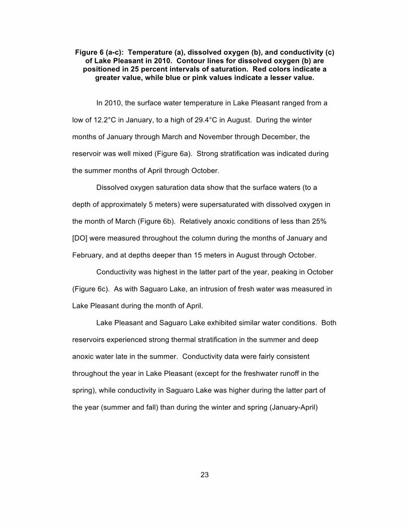
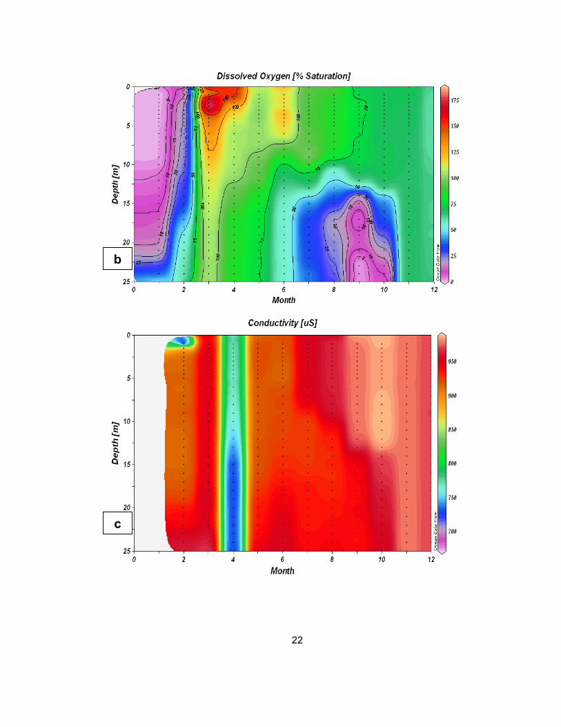
Figure 6 (a-c): Temperature (a), dissolved oxygen (b), and conductivity (c) of Lake Pleasant in 2010. Contour lines for dissolved oxygen (b) are

positioned in 25 percent intervals of saturation. Red colors indicate a greater value, while blue or pink values indicate a lesser value.

In 2010, the surface water temperature in Lake Pleasant ranged from a

low of 12.2°C in January, to a high of 29.4°C in August. During the winter

months of January through March and November through December, the

reservoir was well mixed (Figure 6a). Strong stratification was indicated during

the summer months of April through October.

Dissolved oxygen saturation data show that the surface waters (to a

depth of approximately 5 meters) were supersaturated with dissolved oxygen in

the month of March (Figure 6b). Relatively anoxic conditions of less than 25%

[DO] were measured throughout the column during the months of January and

February, and at depths deeper than 15 meters in August through October.

Conductivity was highest in the latter part of the year, peaking in October

(Figure 6c). As with Saguaro Lake, an intrusion of fresh water was measured in

Lake Pleasant during the month of April.

Lake Pleasant and Saguaro Lake exhibited similar water conditions. Both

reservoirs experienced strong thermal stratification in the summer and deep

anoxic water late in the summer. Conductivity data were fairly consistent

throughout the year in Lake Pleasant (except for the freshwater runoff in the

spring), while conductivity in Saguaro Lake was higher during the latter part of

the year (summer and fall) than during the winter and spring (January-April)

23

Secchi Depth

Figure 7: Secchi depth and estimated euphotic zone depth in Lake Pleasant and Saguaro Lake.

Recorded Secchi depth was consistently deeper in Lake Pleasant than

Saguaro Lake (Figure 7). The deepest Secchi depth recorded in Saguaro Lake

was 3m, the shallowest was 1.25, and the yearly average was 2.06m ± 0.64. In

Lake Pleasant, the deepest recorded Secchi depth was 12m, the shallowest was

2.75m, and the yearly average was 6.125m ± 2.68.

24

0  

5  

10  

15  

20  

25  

1   2   3   4   5   6   7   8   9   10   11   12  Dep

th  (m

)  Month  Secchi  Depth  

Saguaro  Lake  Secchi  

Saguaro  Lake  Eupho:c  Zone  

Lake  Pleasant  Secchi  

Lake  Pleasant  Eupho:c  Zone  

Dissolved Inorganic Nutrients

Table 2: Dissolved inorganic nutrient concentrations Lake Pleasant and Saguaro Lake

25

0.0  

5.0  

10.0  

15.0  

20.0  

25.0  

30.0  

35.0  

40.0  

0.00  

0.20  

0.40  

0.60  

0.80  

1.00  

1.20  

1   2   3   4   5   6   7   8   9   10   11   12  

Nitrogen  (NO3  +  NO2)  (u

mol)  

Phosph

orus  (P

O4)  (u

mol/L)  

Month  

Lake  Pleasant  

Phosphorus  

Nitrogen  

a

Figure 8 (a, b): Dissolved inorganic nutrient concentrations determined in the surface of Lake Pleasant (a), and Saguaro Lake (b). Concentrations are

depicted in micro-moles. Note: Phosphorus and Nitrogen are plotted on separate axes.

26

0.00  

5.00  

10.00  

15.00  

20.00  

25.00  

30.00  

35.00  

40.00  

0.00  

0.05  

0.10  

0.15  

0.20  

0.25  

0.30  

1   2   3   4   5   6   7   8   9   10   11   12  

Nitrogen  (NO3  +  NO2)  (u

mol)  

Phosph

orus  (P

O4)  (u

mol/L)  

Month  

Saguaro  Lake  

Phosphorus  

Nitrogen  

b

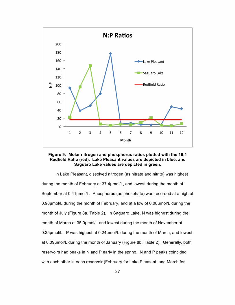
Figure 9: Molar nitrogen and phosphorus ratios plotted with the 16:1 Redfield Ratio (red). Lake Pleasant values are depicted in blue, and

Saguaro Lake values are depicted in green.

In Lake Pleasant, dissolved nitrogen (as nitrate and nitrite) was highest

during the month of February at 37.4µmol/L, and lowest during the month of

September at 0.41µmol/L. Phosphorus (as phosphate) was recorded at a high of

0.98µmol/L during the month of February, and at a low of 0.08µmol/L during the

month of July (Figure 8a, Table 2). In Saguaro Lake, N was highest during the

month of March at 35.0µmol/L and lowest during the month of November at

0.35µmol/L. P was highest at 0.24µmol/L during the month of March, and lowest

at 0.09µmol/L during the month of January (Figure 8b, Table 2). Generally, both

reservoirs had peaks in N and P early in the spring. N and P peaks coincided

with each other in each reservoir (February for Lake Pleasant, and March for

27

0  

20  

40  

60  

80  

100  

120  

140  

160  

180  

200  

1   2   3   4   5   6   7   8   9   10   11   12  

N:P  

Month  

N:P  RaBos  

Lake  Pleasant  

Saguaro  Lake  

Redfield  Ra:o  

Saguaro Lake). N and P concentration peaks in Lake Pleasant declined

throughout the months of March through May, and remained low throughout the

remainder of most of the year. A small peak in N and P was measured at the

very end of the year, during December. N concentrations in Saguaro Lake

declined immediately after the peak during March, and remained low for the

remainder of the year. P concentrations in Saguaro Lake fluctuated throughout

the year, with two additional minor peaks measured during August and

November.

Dissolved nitrogen and phosphorus ratios in Saguaro Lake were above

the Redfield Ratio (Redfield, 1958) during the months of January through March

and the month of September. Subsequently, N:P ratios were below the Redfield

Ratio during the months of April through August and October through December.

N:P ratios in Lake Pleasant were above the Redfield Ratio during the months of

January through May and the months of November/December. N:P ratios were

below the Redfield Ratio in the months of June through October (Figure 9). N:P

ratios above the Redfield Ratio indicate P limitation, while those below the

Redfield Ratio indicate N limitation.

28

Particulate Constituents

Table 3: POC/PON/POP in Lake Pleasant and Saguaro Lake. BDL: Below Detection Limit.

29

Figure 10 (a, b): Particulate P, N, and C values from the surface of Lake Pleasant (a) and Saguaro Lake (b).

30

0  

10  

20  

30  

40  

50  

60  

70  

0  0.2  0.4  0.6  0.8  1  

1.2  1.4  1.6  1.8  2  

1   2   3   4   5   6   7   8   9   10   11   12  

Nitrogen  an

d  Ca

rbon

 (umol)  

Phosph

orus  (u

mol/L)  

Month  

Lake  Pleasant  

Phosphorus  

Nitrogen  

Carbon  

0  20  40  60  80  100  120  140  160  180  200  

0.00  

2.00  

4.00  

6.00  

8.00  

10.00  

12.00  

14.00  

1   2   3   4   5   6   7   8   9   10   11   12  

Carbon

 (umol)  

Phosph

orus  and

 Nitrogen  (umol/L)  

Month  

Saguaro  Lake  

Phosphorus  

Nitrogen  

Carbon  

a

b

Figure 11: Ratios of particulate organic C and N. Lake Pleasant is depicted in blue, Saguaro Lake is depicted in green, and the Redfield Ratio is

depicted in red.

In Lake Pleasant, particulate carbon was recorded at a high of

64.05µmol/L during the month of June, and a low of 8.35µmol/L during the month

of December. Nitrogen was highest during the month of May at 14.60µmol/L,

and a low of 1.67µmol/L during the month of June. Phosphorus was only

recorded above the background during the month of May, at 1.83µmol/L (Figure

10a, Table 3). POC and PON ratios typically were measured above the Redfield

Ratio of 6.6:1, indicating C richness. However, in the months of January,

February, April, and July, POC/PON ratios were measured below Redfield,

indicating N richness. Large spikes in the ratio were measured in the months of

May and August (Figure 11). I could only calculate

31

5  

6  

7  

8  

9  

10  

11  

12  

13  

1   2   3   4   5   6   7   8   9   10   11   12  

C:N  RaB

o  

Month  

C:N  RaBos  

Saguaro  Lake  

Lake  Pleasant  

Redfield  

PON/POP ratios for the month of May, because POP was below detection limit

for all the other months. During the month of May, the PON/POP ratio was 8:1,

below both the Redfield (16:1) and “Elser” (30:1) ratios indicating relatively P rich

particulate matter, which would be more nutritious for Daphnia (who require

greater P, as they are P rich themselves).

In Saguaro Lake, POC was highest during the month of June at

171.43µmol/L and lowest during the month of November at 19.65µmol/L. PON

was recorded at a high of 13.23µmol/L during the month of November, and a low

of 1.27µmol/L during the month of August. POP was only recorded above the

background during the month of November, at 0.24µmol/L (Figure 10b, Table 3).

POC/PON ratios were above the Redfield Ratio for six months of the year:

January, April, June through August, and October. The largest spike was

measured in the month of June (Figure 11). PON/POP ratios could only be

calculated for the month of November, due to the reason stated above. During

the month of November, the PON/POP ratio was 54.8:1, above the Redfield and

“Elser” ratios, indicating relatively N rich particulate matter.

32

Chlorophyll a

33

0  

10  

20  

30  

40  

50  

1   2   3   4   5   6   7   8   9   10   11   12  

Chloroph

yll  (ug

/L)  

Month  

Saguaro  Lake,  Surface  

0  1  2  3  4  5  6  7  

1   2   3   4   5   6   7   8   9   10   11   12  

Chloroph

yll  (ug

/L)  

Month  

Lake  Pleasant,  Surface  

a

b

c

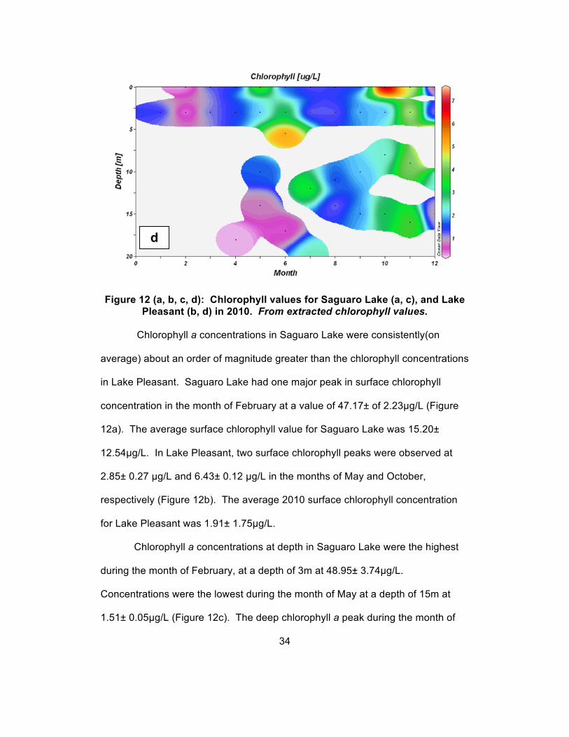
Figure 12 (a, b, c, d): Chlorophyll values for Saguaro Lake (a, c), and Lake Pleasant (b, d) in 2010. From extracted chlorophyll values.

Chlorophyll a concentrations in Saguaro Lake were consistently(on

average) about an order of magnitude greater than the chlorophyll concentrations

in Lake Pleasant. Saguaro Lake had one major peak in surface chlorophyll

concentration in the month of February at a value of 47.17± of 2.23µg/L (Figure

12a). The average surface chlorophyll value for Saguaro Lake was 15.20±

12.54µg/L. In Lake Pleasant, two surface chlorophyll peaks were observed at

2.85± 0.27 µg/L and 6.43± 0.12 µg/L in the months of May and October,

respectively (Figure 12b). The average 2010 surface chlorophyll concentration

for Lake Pleasant was 1.91± 1.75µg/L.

Chlorophyll a concentrations at depth in Saguaro Lake were the highest

during the month of February, at a depth of 3m at 48.95± 3.74µg/L.

Concentrations were the lowest during the month of May at a depth of 15m at

1.51± 0.05µg/L (Figure 12c). The deep chlorophyll a peak during the month of

34

d

February coincides with the surface peak of chlorophyll a concentration. The

deep minor peak during the month of July also coincides with a minor peak in

surface concentrations during the same month. In Lake Pleasant, chlorophyll a

concentrations at depth were the highest during the month of June at a depth of

5.5m at 3.69± 0.11µg/L. Concentrations were the lowest during the month of

April at a depth of 18m at 0.16± 0.004µg/L (Figure 12d). The deep chlorophyll a

peak during the month of June coincides with the estimated euphotic zone depth.

35

Phytoplankton Community

Table 4: Qualitative examination of phytoplankton communities in Lake Pleasant and Saguaro Lake. Specific months were selected due to

coinciding events in zooplankton abundance and peaks in chlorophyll a.

In Lake Pleasant (Table 4), Synechococcus was relatively abundant in six

of the seven months and was the most abundant phytoplankton during three of

the months that it was present (May, August, and November). In May, the

36

cyanobacteria formed large aggregates. In August and November, the

cyanobacteria occurred as individual cocci. Prymnesiophytes were present in

five of the seven months (May through September, and November).

Prymnesiophytes were the most abundant phytoplankton during the month of

July, which experienced the greatest recorded decline of zooplankton abundance

in 2010. Other abundant organisms included pennate diatoms, centric diatoms,

cryptophytes, and chlorophytes. In the months of May and October, large

bundles of wood fibers were found amongst the phytoplankton.

In Saguaro Lake (Table 4), prymnesiophytes were found in every month,

but were never the most abundant phytoplankton. The community was varied

throughout the year, also consisting of centric diatoms, euglenoids, cryptophytes,

and filamentous cyanobacteria. The appearance of the potentially toxic

filamentous cyanobacteria Cylindrospermopsis during the month of July

coincided with a decrease in abundance of all zooplankton. Cylindrospermopsis

remained abundant throughout the rest of the year, and zooplankton population

abundance remained low as well.

37

Zooplankton Abundance

Figure 13: Abundance of zooplankton in the upper 5m of Lake Pleasant during 2010. Values depicted are of individuals per cubic meter.

In Lake Pleasant, zooplankton populations fluctuated over the year of 2010

(Figure 13). All populations experienced a decline in abundance in the month of

July. Observed peaks varied by group. Peaks were measured for copepod

nauplii (cyclopoids and calanoids) during March (3.4x104 ± 2116 m-3), August

(3.06x104 ± 4245 m-3), and November (3.31x104 ± 3012 m-3). Calanoid copepod

peaks occurred in February (1.20x104 ±1324 m-3), May (2.39x104 ± 4407 m-3),

and November (1.79x104 ± 1982 m-3). Cyclopoid copepod peaks were measured

in June (1.08x104 ± 1997 m-3) and November (1.51x104 ± 1579 m-3). Abundance

38

0  

5000  

10000  

15000  

20000  

25000  

30000  

35000  

40000  

1   2   3   4   5   6   7   8   9   10   11   12  

Abu

ndan

ce  (p

er  m

3)  

Month  

Lake  Pleasant  Calanoid  

Cyclopoid  

Nauplii  

Daphnia  

Bosmina  

Diaphanosoma  

of the Cladoceran Daphnia peaked in April (1.33x104 ± 1330 m-3). The

cladoceran Bosmina peaked in April (2.35x103 ± 668 m-3) and August (4.24x103 ±

793 m-3). The cladoceran Diaphanosoma peaked in October (1.79x104 ± 2588).

Nauplii were the greatest in abundance in the zooplankton community, with an

approximate population of 3.3,x104 m-3 in the months of March and November.

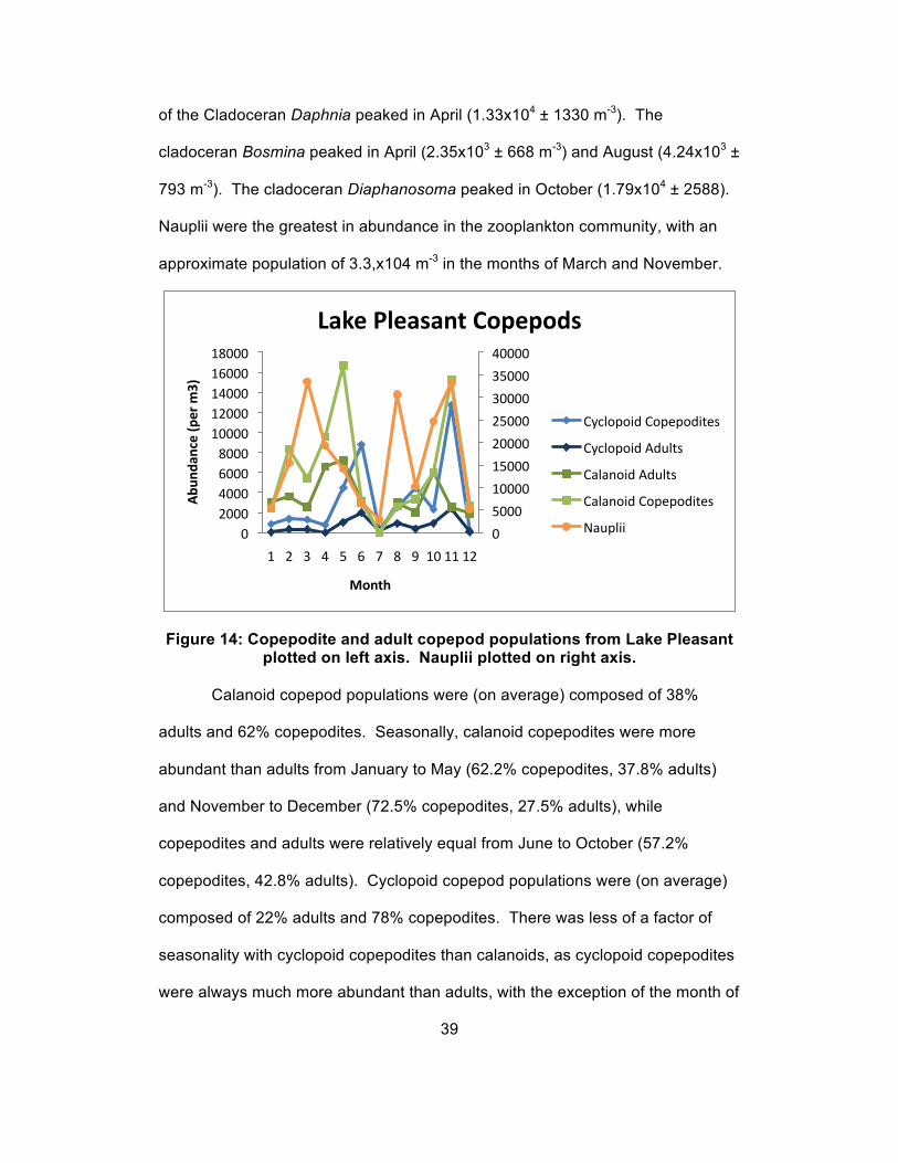
Figure 14: Copepodite and adult copepod populations from Lake Pleasant plotted on left axis. Nauplii plotted on right axis.

Calanoid copepod populations were (on average) composed of 38%

adults and 62% copepodites. Seasonally, calanoid copepodites were more

abundant than adults from January to May (62.2% copepodites, 37.8% adults)

and November to December (72.5% copepodites, 27.5% adults), while

copepodites and adults were relatively equal from June to October (57.2%

copepodites, 42.8% adults). Cyclopoid copepod populations were (on average)

composed of 22% adults and 78% copepodites. There was less of a factor of

seasonality with cyclopoid copepodites than calanoids, as cyclopoid copepodites

were always much more abundant than adults, with the exception of the month of

39

0  

5000  

10000  

15000  

20000  

25000  

30000  

35000  

40000  

0  2000  4000  6000  8000  

10000  12000  14000  16000  18000  

1   2   3   4   5   6   7   8   9   10  11  12  

Abu

ndan

ce  (p

er  m

3)  

Month  

Lake  Pleasant  Copepods  

Cyclopoid  Copepodites  

Cyclopoid  Adults  

Calanoid  Adults  

Calanoid  Copepodites  

Nauplii  

December, when the population was composed of 34% copepodites and 66%

adults. Nauplii were not distinguished as either calanoids or cyclopoids due to

difficulties in identifying the two groups. As a whole (averaged) nauplii made up

55% of the total copepod community throughout the year. Nauplii populations

generally peaked during months of low abundance of other copepod copepodites

and adults (March and August), with the exception of November, when nauplii

abundance peaked along with both cyclopoid and calanoid copepodites (Figure

14).

Figure 15: Abundance of zooplankton in the upper 5m of Saguaro Lake during 2010. Values depicted are of individuals per cubic meter. Note: Cyclopoids/Daphnia, nauplii, and Bosmina are plotted on different axes.

Saguaro Lake (Figure 15) had a less abundant copepod and Daphnia

community than Lake Pleasant (Figure 13). However, nauplii and Bosmina in

Saguaro Lake were more abundant (at their peak) than in Lake Pleasant.

Saguaro Lake zooplankton populations were more abundant in the first half of

the year (winter and spring), and began to decline steadily during the summer.

Populations of cyclopoid copepodites (9.78x103 m-3 ±1 798), nauplii

40

(2.16x105 m-3 ± 7759), and the cladoceran Bosmina (4.72x104 m-3 ± 3965)

peaked in the months of March and April. The cladoceran Daphnia (1.13x104 m-3

± 119) peaked in the month of July.

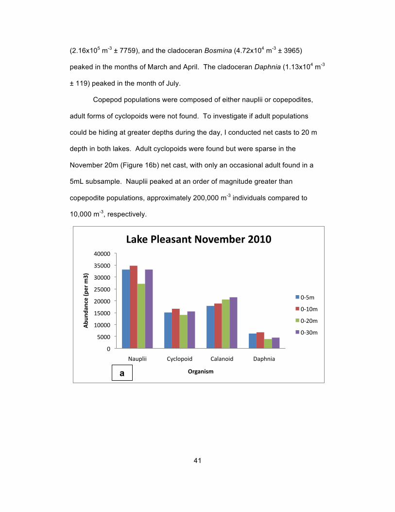
Copepod populations were composed of either nauplii or copepodites,

adult forms of cyclopoids were not found. To investigate if adult populations

could be hiding at greater depths during the day, I conducted net casts to 20 m

depth in both lakes. Adult cyclopoids were found but were sparse in the

November 20m (Figure 16b) net cast, with only an occasional adult found in a

5mL subsample. Nauplii peaked at an order of magnitude greater than

copepodite populations, approximately 200,000 m-3 individuals compared to

10,000 m-3, respectively.

41

0  

5000  

10000  

15000  

20000  

25000  

30000  

35000  

40000  

Nauplii   Cyclopoid   Calanoid   Daphnia  

Abu

ndan

ce  (p

er  m

3)  

Organism  

Lake  Pleasant  November  2010  

0-­‐5m  

0-­‐10m  

0-­‐20m  

0-­‐30m  

a

Figure 16 (a, b): Comparison of abundance estimates derived from casts of different depth intervals from Lake Pleasant and Saguaro Lake in

November. Nested columns represent different organisms while each color represents a different depth interval. Copepod data represents combined

adults and copepodites.

In Lake Pleasant (Figure 16a), abundance of nauplii was similar from 0-

5m, 0-10m, and 0-30m. Nauplii from 0-20m were less abundant than the other

three depths. Cyclopoid copepods were relatively well distributed throughout the

water column. Calanoid copepods became more abundant as depth increased

down to the maximum sample depth of the 30m net cast. The cladoceran

Daphnia was most abundant from 0-5m and 0-10m, while less abundant from 0-

20m and 0-30m. The cladoceran Bosmina was not present in significant

numbers at any depth in the month of November.

In Saguaro Lake (Figure 16b) the nauplii population was distributed

relatively equally in the upper 20m. Cyclopoid copepod abundance increased

steadily with increasing depth, indicating that populations were more abundant in

deeper depths. Cladocerans Bosmina and Daphnia both declined as sampling

42

b

reached deeper depths, indicating that they were more concentrated in the upper

5m of the water column.

Zooplankton Biomass

Figure 17 (a, b): Zooplankton biomass in Lake Pleasant and Saguaro Lake. Saguaro Lake Bosmina plotted on right axis (b).

43

0  20  40  60  80  

100  120  140  160  180  200  

1   2   3   4   5   6   7   8   9   10   11   12  

Biom

ass  (m

g/m3)  

Month  

Lake  Pleasant   Calanoid  

Cyclopoid  

Daphnia  

Bosmina  

Diaphanosoma  

0  

10  

20  

30  

40  

50  

60  

0  1  2  3  4  5  6  7  8  9  10  

1   2   3   4   5   6   7   8   9   10   11   12  

Biom

ass  (m

g/m3)  

Month  

Saguaro  Lake  

Cyclopoid  

Daphnia  

Bosmina  

b

a

Biomass of zooplankton in Lake Pleasant (Figure 17a) and Saguaro Lake

(Figure 17) followed patterns similar to abundance figures (Figures 13 and 15).

Two exceptions are the Daphnia populations in either reservoir. In Lake

Pleasant, there was more Daphnia biomass than calanoid biomass during the

month of April despite greater calanoid abundance. Daphnia in Lake Pleasant

were very large throughout the year (body length average of 1200µm ± 112). In

Saguaro Lake, Daphnia biomass also deviates from the pattern of abundance

during the month of July. This is due to the small size of Daphnia during July

with an average body length of 550µm ± 213 compared to the average body

length during all other months of 900µm ± 239. In addition to the small size of

Daphnia in Saguaro Lake, the helmets and tails of individuals formed elongated

spikes, along with the spines on the carapace. The Daphnia of Lake Pleasant

did not have any of these features.

Rotifer Abundance

Figure 18: Rotifer abundance in Saguaro Lake from June to November of 2010.

44

0  

50000  

100000  

150000  

200000  

250000  

6   7   8   9   10   11  

Abu

ndan

ce  (p

er  m

3)  

Month  

Saguaro  Lake  

Ro:fers  

Rotifer abundance of Saguaro Lake (Figure 18) was determined only

during the months of June through November in the euphotic zone (Figure 7).

They were the most abundant during the month of June (2.34x105 m-3 ±

3.32x104), and least abundant during the month of July (3 m-3 ± 2.82). The

average abundance of rotifers was 8.24 x 104 m-3 ± 8.28x104 for the study period.

The average from August through November was 5.27x 104 m-3 ± 3.91x104.

Lake Pleasant Fish Community (AZGFD 2005 and 2008)

From data in two separate studies, the fish community of Lake Pleasant

was composed of the following fish: Striped Bass (Morone saxatilis), White Bass

(Morone chrysops), Largemouth Bass (Micropterus salmoides), Green Sunfish

(Lepomis cyanellus), Bluegill (Lepomis macrochirus), Redear Sunfish

(Lepomis microlophus), Sunfish Hybrid (Lepomis sp.), White Crappie (Pomoxis

annularis), Black Crappie (Pomoxis nigromaculatus), Channel Catfish (Ictalurus

punctatus), Flathead Catfish (Pylodictis olivaris), Tilapia (Tilapia sp.), Common

Carp (Cyprinus carpio), Goldfish (Carassius auratus), Threadfin Shad (Dorosoma

petenense), Golden Shiner (Notemigonus crysoleucas), Red Shiner (Cyprinella

lutrensis), Mosquitofish (Gambusia affinis), Yellow Bullhead (Ameiurus natalis),

and Sonora Sucker (Catostomus insignis) (Bryan, 2005; Stewart et al., 2008).

From 2000 to 2003, Arizona Game and Fish found that the average

individual mass of Striped Bass decreased. From 2000 to 2006, average

individual mass of Striped Bass (large piscivore), while the average individual

mass of Threadfin Shad (planktivore) increased (Bryan, 2005) (Stewart et al.,

2008).

Populations of Striped Bass individuals had the greatest mass in 2004 of

1334g (August specifically), and the lowest mass in 2005 of 333g (August

45

specifically). Populations of Threadfin Shad individuals had the greatest mass in

2006 (70g), and the lowest mass in 2000 (9g). The decreasing mass of

individual Striped bass indicates that overall population abundance increased

over time, due to intra-specific competition and stunted growth of the fish

(Amundsen et al., 2007).

Saguaro Lake Fish Community

AZGFD (2011c) reports the following fish in Saguaro Lake: Rainbow

Trout (Oncorhynchus mykiss), Largemouth Bass (Micropterus salmoides),

Smallmouth Bass (Micropterus dolomieu), Yellow Bass (Morone

mississippiensis), Crappie (Pomoxis sp.), Sunfish (Lepomis sp.), Channel Catfish

(Ictalurus punctatus), Tilapia (Tilapia sp.), and Yellow Perch (Perca flavescens).

Saguaro Lake receives period stockings of the

planktivore/insectivore/piscivore Rainbow Trout throughout the winter months.

However, in 2010, stockings were scaled back (AZGFD 2011d). The large

piscivores Largemouth and Smallmouth Bass are not stocked in Saguaro Lake,

and are not found in the density of Striped Bass in Lake Pleasant. Furthermore,

these piscivores are benthic and not pelagic, and occur mainly in the shallow

parts of the reservoirs closer to the shore.

DNA Based Molecular Gut Analyses

Molecular examination yielded results from the gut content of

selected animals and the water column. Results were quantified by the density

of DGGE bands (denser bands indicate a higher concentration of DNA). Results

labeled “Other” belong to DGGE bands that were not sequenced and do not have

an equivalent band on the specific DGGE gel. The “Other” bands may be the

46

DNA of the animal itself, or unidentified prey bands. Cyanobacterial sequences

were not obtained, due to insufficient extraction using the Qiagen kit.

Saguaro Lake

In Saguaro Lake, results were obtained from successfully amplified

cyclopoid copepodite, cyclopoid nauplii and Daphnia guts. No DNA sequences

were successfully amplified from Bosmina guts.

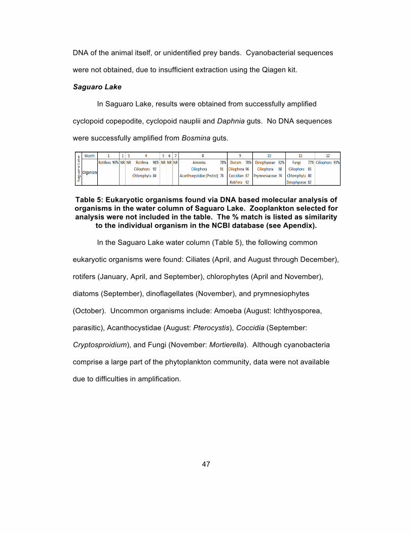
Table 5: Eukaryotic organisms found via DNA based molecular analysis of organisms in the water column of Saguaro Lake. Zooplankton selected for analysis were not included in the table. The % match is listed as similarity

to the individual organism in the NCBI database (see Apendix).

In the Saguaro Lake water column (Table 5), the following common

eukaryotic organisms were found: Ciliates (April, and August through December),

rotifers (January, April, and September), chlorophytes (April and November),

diatoms (September), dinoflagellates (November), and prymnesiophytes

(October). Uncommon organisms include: Amoeba (August: Ichthyosporea,

parasitic), Acanthocystidae (August: Pterocystis), Coccidia (September:

Cryptosproidium), and Fungi (November: Mortierella). Although cyanobacteria

comprise a large part of the phytoplankton community, data were not available

due to difficulties in amplification.

47

Figure 19 (a-c): Relative distribution of cyclopoid prey organisms in Saguaro Lake obtained from molecular gut analysis. Data were

successfully obtained from samples collected in May (a), June (b), and December (c). Percentages represent DNA density.

Cyclopoid gut sequences were successfully amplified for three months:

May, June, and December (Figure 19 a-c). In all three months ciliates were

present in the gut data, comprising 6% to 25% of DNA density. In May and June,

dinoflagellate sequences were found at approximately 13% (averaged). In June

48

25%  

9%  

11%  

55%  

May  Cilliate   Chlorophyte  

Dinoflagellate   Other  

6%  

36%  

20%  

15%  

23%  

June  Cilliate   Ro:fer  

Calanoid   Dinoflagellate  

Other  11%  

11%  

78%  

December  Cilliate     Calanoid   Other  

a

b c

and December, calanoid sequences represented 20% and 11% of DNA density,

respectively. Chlorophytes were only found in the gut data in May (9%), while

rotifers were only found in June (36%).

49

17%  

9%  

7%  67%  

May  Cilliate   Ro:fer  

Chlorophtye   Other  

20%  

16%  64%  

June  Cilliate  

Dinoflagellate  

Other  

20%  

48%  

32%  

August  Cilliate   Other   Ro:fer  

a

b c

Figure 20 (a-g): Nauplii (Cyclopoid) prey organisms in Saguaro Lake. Data obtained from molecular gut analysis. Data were successfully obtained from samples collected in May (a), June (b), August (c), September (d),

October (e), November (f), and December (g). Percentages represent DNA density.

Nauplii gut sequences were successfully amplified for the months of May,

June, August, September, October, November, and December (Figure 20 a-g).

In the later months of 2010 rotifer sequences were abundant in the guts,

and in September, 78% of all amplified DNA were rotifer sequences. Ciliate

50

78%  

9%  

13%  

September  Ro:fer   Cilliate   Other  

44%  

56%  

October  Ro:fer   Other  

12%  

39%  

49%  

November  Pro:st   Ro:fer   Other  

10%  

28%  

62%  

December  Pro:sts   Ro:fer   Other  

d e

f g

sequences were found in four out of the seven months, no ciliate sequences

were successfully amplified in October, November, or December. Chlorophyte

sequences were found in May, while dinoflagellate sequences were found in

June. Various other protists were found in November and December.

Figure 21: Daphnia prey organisms in Saguaro Lake. Data obtained from molecular gut analysis. Data were only successfully obtained from

samples collected in May. Percentages represent DNA density.

Sequences from Daphnia guts were only successfully amplified in the

month of May (Figure 21). Ciliates comprised of the majority of known

sequences. Chlorophytes and rotifers were also found.

51

17%  

7%  

9%  

67%  

May  Daphnia  Cilliate   Chlorophyte   Ro:fer   Other  

Lake Pleasant

In Lake Pleasant animals selected for examination were: Cyclopoids,

calanoids, nauplii, Daphnia, Diaphanosoma, and Bosmina. Gut DNA was

successfully amplified from cyclopoids, calanoids, nauplii, and Bosmina.

Amplification of guts was not successful for Daphnia or Diaphanosoma.

Table 6: Eukaryotic organisms found via DNA based molecular analysis of the organisms in the water column of Lake Pleasant. Zooplankton selected

for analysis are not included here. The % match is listed as similarity to the individual organism in the NCBI database (see Apendix).

In the Lake Pleasant water column (Table 6), the following common

eukaryotic organisms were found: Chlorophytes (February), ciliates (February,

April, and August through December), dinoflagellates (April, August, and

September), rotifers (August), and diatoms (October). Uncommon eukaryotic

organisms include: Apicocomplexa (February and September: parasitic phyla),

Coccidia (February: Cryptosporidium), Kinetoplastida (July), Spizellomycetales

(July: fungi), Spermatophyta (July: seed plants), Rhizidiomycetaceae (August:

Chromista), Bicosoecidae (August), Codonosigidae/Choanoflagellida

(August/December), stramenopiles (October and November: oomycetes),

Rhizaria (November: Cercomonadida), and fungi (November: Candida).

Although cyanobacteria comprise a large part of the phytoplankton community,

data were not available due to difficulties in amplification.

52

53

27%  

17%  39%  

17%  

June  Cilliate   Ro:fer  

Calanoid   Other  

45%  

46%  

9%  

July  Cilliate   Calanoid   Other  

35%  

27%  

38%  

August  Pro:st   Ro:fer   Other  

88%  

12%  

November  Calanoid   Other  

a b

c d

Figure 22 (a-e): Cyclopoid prey organisms in Lake Pleasant from molecular gut analysis. Data were successfully obtained from samples collected in

June (a), July (b), August (c), November (d), and December (e). Percentages represent DNA density.

Cyclopoid gut data were amplified successfully for five months (Figure 22

a-e). In June, July, and November calanoid sequences made up the majority of

sequences, indicating that the cyclopoids which are known carnivores, preyed

either on pieces of adult or entire nauplii of the calanoids.. Ciliate sequences

were found in June, July, and December. Rotifers were found in June and

August, while various protists were found in August and December.

54

22%  

13%  65%  

December  Cilliate     Pro:st   Other  

e

Figure 23: Calanoid prey organisms in Lake Pleasant from DNA based molecular gut analysis. Data were only successfully obtained from

samples collected in June. Percentages represent DNA density.

Calanoid sequences only amplified in June (Figure 23). In June, ciliates

made up 48% of the amplified DNA, with choanoflagellates making up 28%, and

unknown (eukaryotic) DNA comprising the remaining 24% of the DNA density.

55

28%  

48%  

24%  

June  Choanoflagellate  

Cillate  

Other  

Figure 24 (a, b): Nauplii (Cyclopoid and Calanoid) prey organisms in Lake Pleasant from DNA based molecular gut analysis. Data were successfully obtained from samples collected in July (a), and August (b). Percentages

represent DNA density.

Nauplii sequences were only successfully amplified in the months of July

and August (Figure 24 a, b). In July, ciliates made up the majority of amplified

DNA, while rotifers dominated in August.

56

19%  

45%  

36%  

July  Proporata   Cilliate   Other  

59%  

41%  

August  Ro:fer   Other  

a b

Figure 25 (a, b): Bosmina prey organisms in Lake Pleasant from DNA based molecular gut analysis. Data were successfully obtained from samples collected in August (a), and September (b). Percentages represent DNA

density.

In Lake Pleasant, only Bosmina gut sequences were successfully

amplified (Figure 25 a, b), there were no data for Daphnia guts. In Bosmina,

rotifers were found in the month of August, while calanoids were found in August

and September.

57

24%  

10%  66%  

August  Bosmina  Ro:fer   Calanoid   Other  

51%  49%  

September  Bosmina    Calanoid   Other  

a b

Discussion

Lake Pleasant and Saguaro Lake differed in the following four ways: 1)

Lake Pleasant had a dissolved inorganic P concentration an order of magnitude

greater than Saguaro Lake. Dissolved inorganic N concentration peaks were

similar between the two reservoirs, but Lake Pleasant had high N concentrations

after the initial peak for three months longer than Saguaro Lake. 2) Chlorophyll a

concentrations (surface) in Saguaro Lake were approximately nine times greater

than those in Lake Pleasant, and as a consequence, Saguaro Lake was more

turbid than Lake Pleasant. Light is estimated to penetrate approximately five

times deeper in

Lake Pleasant than Saguaro Lake. 3) Zooplankton abundance and biomass in

Lake Pleasant was much greater than in Saguaro Lake. There are also a greater

number of zooplankton groups in Lake Pleasant than Saguaro Lake. 4) Lake

Pleasant contains the large pelagic piscivore Striped Bass. This species is not

present in Saguaro Lake. The following discussion is split into six sections: 1)

Hydrographical context. 2) Seasonal zooplankton variability in the reservoirs in

relation to phytoplankton variability. 3) Food webs of the reservoirs derived from

gut analyses and literature. 4) Controls of community structure. 5) Hypothesis

evaluation. 6) Future work.

1. Hydrographical Context

In the Winter and early Spring of 2010 (January through March), Central

Arizona experienced approximately 330mm (13 inches) of precipitation (NWS,

2011). This period of precipitation coincides with increased dissolved nitrogen

levels and decreased conductivity in both reservoirs, possibly due to the influx of

runoff of freshwater (as seen in the decreased conductivity, Figures 5c and 6c).

58

In the months of February and March chlorophyll a values in Saguaro Lake

increased by an order of magnitude, coinciding with the increase in dissolved

inorganic nitrogen. However, both reservoirs experienced turnover at this time,

so the increased nitrogen may be due to mixing of nutrient-rich deep waters as

well. Lake Pleasant did not see a simultaneous response in chlorophyll values

coinciding with increased nitrogen or the increased runoff of winter and early

spring.

In the spring and early summer of 2010 (March through May) incomplete

stratification coincided with deep penetration of dissolved oxygen in Saguaro

Lake and Lake Pleasant (Figures 5b and 6b).

In the summer and early fall of 2010 (June through October) strong

thermal stratification prevented mixing of the water column with respect to

dissolved oxygen. As a result, a large area of depleted oxygen or anoxic water

developed at depth in the water column. In Lake Pleasant specifically, this area

of anoxic water was found much deeper, due to the increased clarity of the water

and penetration of solar radiation fueling primary production. The anoxic area

was shallower by comparison in Saguaro Lake due to the inability of solar

radiation to penetrate deep into the reservoir.

In the fall and early winter of 2010 (November and December) Lake

Pleasant (Figure 26a) and Saguaro Lake (Figure 26b) turned over and became

well-mixed. The mixing of nutrient-rich (both N and P) deep water at the surface

did not lead to increases in chlorophyll in Lake Pleasant. In Saguaro Lake,

however, the deep water mixing coincided with minor peaks in P concentration,

and subsequent increases in chlorophyll a, with minor peaks during November

and December. Chlorophyll values in Lake Pleasant began to decrease from the

59

peak measured in the month of October. During this November decrease in

chlorophyll, the dissolved N:P ratio increased above the Redfield Ratio, indicative

of phosphorus limitation. Phosphorus limitation limits primary production.

Figure 26 (a, b): Covariation of temperature, chlorophyll, and nitrogen in Lake Pleasant (a) and Saguaro Lake (b).

60

a

b

2. Seasonal Zooplankton Variability in the Reservoirs in Relation to

Phytoplankton Variability

The zooplankton community in Lake Pleasant was more diverse than the

community in Saguaro Lake, two additional groups of zooplankton (calanoid

copepods and the cladoceran Diaphanosoma) were found in Lake Pleasant.

Additionally, zooplankton biomass was higher in Lake Pleasant than in Saguaro

Lake. Populations of zooplankton were found in abundance throughout 2010 in

Lake Pleasant, while Saguaro Lake experienced a decline in the second half of

2010 (Figure 13 and 15).

In the month of July, all populations of zooplankton in Lake Pleasant

decreased sharply. This might have been correlated with a seasonal variation in

the phytoplankton population: 1) There was a prymnesiophyte bloom in July.

The toxin produced by certain prymnesiophytes (Prymnesium, for example) may

render them inedible or poisonous. This is consistent with results found by

Remmel et al. (2011), reporting that populations of Daphnia began to decline

after ten days of exposure to toxic prymnesiophytes. 2) The cyanobacteria

Synechococcus was not forming aggregates, but was found in small clumps

(three or four cells) or individually. When not in aggregate, the individual cells

may be too small to consume.

The following might also contribute to the decrease of abundance

observed in July in Lake Pleasant: 1) Predation on zooplankton by planktivorous

fish such as the Threadfin Shad may have temporarily increased. DeVries et al.

(1991) found that when Threadfin Shad populations peaked in Stonelick Lake,

Ohio, zooplankton populations experienced massive declines. 2) Populations of

zooplankton were possibly at a deeper depth than the deepest (10m) vertical tow

61

performed at the time of collection. Diel migration of the populations were not

studied extensively; only one significantly deep tow (30m) was performed during

the month of November. From the November deep results (20m and 30m), we

see that large populations of zooplankton do occupy the water column well under

the estimated euphotic zone (Figures 7 and 16a) in Saguaro Lake. Mcnatt

(1977) found large diel migrations of zooplankton in Canyon Lake and Apache

Lake of the Salt River chain.

After the month of April, all zooplankton populations in Saguaro Lake

decreased from a peak in abundance in the month of March. From the months of

July through December, all populations were very low in abundance. This might

have been correlated with the following changes observed in the phytoplankton:

Prymnesiophytes were found in greater abundance in the months of July through

November. The effects of prymnesiophytes on zooplankton would be the same

as listed above, for Lake Pleasant. Also in the time period of July through

November, filamentous cyanobacteria (Cylindrospermopsis, Aphanizomenon)

were abundant in the phytoplankton community. Existing literature indicates that

these filamentous cyanobacteria release toxins to inhibit competition amongst

phytoplankton and to inhibit grazing by zooplankton (DeMott and Moxter, 1991).

Variable N:P ratios of phytoplankton can have significant effects on a food

web, as low phosphorus phytoplankton are considered to be of low nutritional

quality for zooplankton- especially for the cladoceran Daphnia which has a high

requirement for phosphorus (Elser et al, 2000). The difference in nutrient load

and stoichiometric ratios of dissolved inorganic nitrogen to phosphorus (N:P)

should influence the stoichiometric ratios (PON:POP) of phytoplankton and would

constitute a form of bottom-up control of the plankton community. High dissolved

62

inorganic N:P ratios during the month of May in Lake Pleasant indicate P

limitation. However, during the month of May, the ratio of PON:POP was 8:1

(Table 2), indicating P-rich phytoplankton. These P-rich phytoplankton would be

excellent nutrition for Daphnia populations, but during the month of May, Daphnia

abundance was only average (Figure 13). This may be evidence for bottom-up

control or possibly an effect of competition, as there was also a peak in the

population of calanoid copepods during the month of May. During the month of

November in Saguaro Lake, the PON:POP ratio was 55:1, higher than the

Redfield and “Elser” ratios, indicating N-rich phytoplankton. Dissolved inorganic

N:P for November in Saguaro Lake was below the Redfield ratio indicating N

limitation, which coincides with the presence of filamentous cyanobacteria

(Table 2). This may be further evidence for bottom-up control of the community

in Saguaro Lake. To further describe phytoplankton nutritional value, a more

complete particulate P data set would be required.

63

3. Food Webs in the Reservoirs Derived from Gut Analyses and Literature

Figure 27: Hypothesized and inferred food web of Lake Pleasant. Black boxes and directional arrows depict relationships hypothesized from

literature. Blue boxes depict taxonomic groups selected for DNA based molecular gut analyses. Red boxes depict prey organism groups found

through DNA based molecular gut analyses. Red directional arrows represent inferred energy pathways, from DNA based molecular gut analyses. Larger groupings such as Zooplankton, Crustaceans, and

Phytoplankton are presented based on descriptions of trophic interactions from literature.

In Lake Pleasant, five distinct trophic levels were identified (Figure 27).

The lowest of these is made up of primary producer phytoplankton and bacteria.

The first consumer level is made up of grazer zooplankton (first order

consumers) and carnivore zooplankton (second order consumers). This second

tier feed upon the first tier of producers (DeMott, 1982; Kagami et al., 2002; von

Elert et al., 2003; Maly and Maly, 1974; Hansen and Hairston, 1998), and

amongst itself in the case of carnivorous cycloploids and omnivorous calanoids

64

(DeMott, 1982; Kerfoot, 1987; Maly and Maly, 1974; Elser et al., 1995; Hansen

and Hairston, 1998). This tier of zooplankton is more diverse in Lake Pleasant

than in Saguaro Lake, with six (including nauplli, not pictured in Figure 27)

groups of crustacean zooplankton. Saguaro Lake only possesses four (three

pictured in Figure 28, nauplii are not pictured) groups of zooplankton. Note: all

inferred trophic linkages (in red, from DNA based molecular analyses) are

contained within the second tier of Figure 27. The third tier is comprised of

planktivores (either second order consumers or third order consumers, based on

the path of energy transfer through the tiers). The juvenile gamefish and

Threadfin Shad feed upon the zooplankton of the second tier (Prophet, 1988),

while the Tilapia feed on a mix of zooplankton and phytoplankton (Gu et al.,

1997; Gido, 2001; Michewicz et al., 1972). The fourth tier is composed of large

piscivore fish (Elser et al., 1995), the Largemouth Bass and Striped Bass.

Currently, Striped Bass are very abundant in Lake Pleasant, to the point of out-

competing the Largemouth Bass (Stewart et al., 2008) and drawing the attention

of the Arizona Game and Fish Department. AZGFD has currently (as of 2011)

lifted any sort of harvest limit on Striped Bass in an effort to manage their

numbers (AZGFD, 2011b). The apex of the food web is occupied by piscivore

raptors, the Osprey and Bald Eagle (Haywood and Ohmart, 1986) as well as

humans.

65

Figure 28: Hypothesized and inferred food web of Saguaro Lake. Black boxes and directional arrows depict relationships hypothesized from

literature. Blue boxes depict taxonomic groups selected for DNA based molecular gut analyses. Red boxes depict prey organism groups found

through DNA based molecular gut analyses. Red directional arrows represent inferred energy pathways, from DNA based molecular gut analyses. Larger groupings such as Zooplankton, Crustaceans, and

Phytoplankton are presented based on descriptions of trophic interactions from literature.

In Saguaro Lake, five trophic levels were also identified (Figure 28). The

first tier of primary producers differs from Lake Pleasant as filamentous

cyanobacteria are found in Saguaro Lake. The second tier is less diverse than

Lake Pleasant, lacking the omnivorous calanoids and cladoceran grazer

Diaphanosoma. The third tier differs as Tilapia were not present in Saguaro

Lake (as of 2011, AZGFD indicates only “occasional” reports of Tilapia). The

fourth tier of large fish differs as Striped Bass are not found in Saguaro Lake.

66

However, the cold-water species Rainbow Trout is heavily stocked throughout

the winter. The Rainbow Trout is a piscivore and planktivore. Similar to Lake

Pleasant, piscivore raptors (Bald Eagles and the Osprey) and humans are the

top carnivores in the Saguaro Lake food web.

It should be noted that differences existed between the food webs for

each reservoir. The pelagic community of Saguaro Lake was less diverse than

the pelagic community of Lake Pleasant. The greatest difference was the

occurrence of the large pelagic piscivore, the striped bass, in Lake Pleasant.

This large piscivore biomass near the top level of the food web exerted pressure

on lower trophic levels resulting in a trophic cascade that affected all other

organism groups (see below). The occurrence of omnivorous calanoid copepods

and the herbivorous cladoceran Diaphanosoma in Lake Pleasant represented

new, third and forth, large crustacean grazer groups in the food web, when

compared to Saguaro Lake. These additional populations of grazers also

exerted pressure on lower trophic levels, further strengthening any associated

trophic cascades.

4. Controls of Community Structure

Trophic cascades were described by Carpenter et al. (1985) as the

following: Large stocks of piscivores place enough pressure on planktivores to

reduce biomass of the planktivores. The decrease in planktivore biomass allows

herbivore biomass to increase. The increase in herbivore biomass leads to a

decrease in phytoplankton biomass.

Lake Pleasant has a large population of picivorous striped bass

positioned near the top of the trophic levels. This large amount of biomass in the

upper trophic levels is evidence for a top-down control scheme. The large

67

abundance of striped bass (piscivore) (AZGFD: Bryan, 2005; Stewart et al. 2008)

reduces the abundance of threadfin shad (planktivore). The reduction in

threadfin shad allows the Daphnia, Diaphanosoma, and Calanoid (all herbivores)

to increase. The large amount of herbivore biomass reduces the amount of

phytoplankton (primary producer).

Saguaro Lake has a large biomass of primary producers which is

evidence for a bottom-up control scheme and little top-down control. The smaller

numbers of largemouth and yellow bass (piscivore) allows a relatively greater

threadfin shad (planktivore) abundance. The large amount of threadfin shad

reduces the biomass of Daphnia and Bosmina (herbivores). With reduced

herbivore biomass, there is a large amount of phytoplankton (primary producer)

biomass. The high predation on Daphnia by the Threadfin Shad also explains the

small size of the Daphnia in Saguaro Lake (compared to Lake Pleasant), and the

appearance of large helmet, tail, and carapace spines as predator deterrent..

High turbidity in each reservoir was partly due to blooms of

phytoplankton. Reservoirs such as Lake Pleasant, with abundant large

piscivores and the resulting trophic cascade (described above), had lesser

amounts of phytoplankton biomass than reservoirs with trophic cascades similar

to Saguaro Lake. The smaller amount of phytoplankton biomass correlates with

lesser turbidity than reservoirs that contain greater amounts of phytoplankton

biomass.

5. Hypothesis Evaluation

1) Top-down control varied between the two reservoirs. The presence of a

piscivore in a reservoir determines the amount of grazer and primary producer

biomass through trophic cascades. The data support this hypothesis. According

68

to the principles outlined by Carpenter (1985), Lake Pleasant is a good example

of a community that is controlled from the top-down. This was evident by the

high abundance of piscivore fish. The resulting trophic cascade would indicate a

large zooplankton population (Figure 13) and a small amount of biomass of

primary producers, as was inferred by chlorophyll a values in Figure 12 (b, d).

Conversely, Saguaro Lake was controlled from the bottom-up by the nutrients of

the reservoir. With the large amount of biomass at the primary producer level

(chlorophyll a values, Figure 12a, c), the resulting cascade indicated a small

grazer population (Figure 15) and a small piscivore fish population (evident by

intensive AZGFD stocking of Rainbow Trout, which is not decimated by

piscivores). DNA based molecular data from omnivorous calanoid copepods in

(Figure 23) indicated predation on other zooplankton, a possible result of

competition with cladoceran grazers Daphnia and Bosmina over scarce

phytoplankton (Figure 27). Instead, the cyclopoid copepods in Saguaro Lake

were found to be omnivores, grazing on phytoplankton and preying on other

zooplankton (Figures 28 and 19)

2) Nutrient loads differ for each reservoir. Greater nutrient concentrations yield

greater primary producer biomass. My data lead me to reject this hypothesis.

Saguaro Lake was not more eutrophic compared to Lake Pleasant as originally

expected. Dissolved inorganic phosphorus concentrations in Lake Pleasant were

an order of magnitude greater than those in Saguaro Lake. Additionally, high

levels of dissolved inorganic nitrogen were found for three months after the

winter/spring peak in Lake Pleasant, where there was only a winter/spring peak

of N in Saguaro Lake (Figure 8). The unused stock of nutrients in Lake Pleasant

provides further support for top-down control (see above). According to the

69

Redfield Ratio (16:1 N:P), Saguaro Lake was N limited for 8 months of the year,

while Lake Pleasant was N limited for 5 months. According to the “Elser” ratio

(30:1 N:P), Saguaro Lake was N limited 10 months out of the year while Lake

Pleasant remained N limited for 5 months. The N limitation in Saguaro Lake

allowed the filamentous cyanobacteria (as was seen in previous investigations,

Figure 3) to gain an ecological edge over eukaryotic algae, and dominate the

phytoplankton community. This was not seen in Lake Pleasant as N limitation

does not benefit the dominant cyanobacteria, Synechococcus, as it cannot

readily fix nitrogen. Particulate P data would (if the data were available) indicate

the nutritional value of phytoplankton for Daphnia. The small size and biomass

of Daphnia in Saguaro Lake could be an effect of bottom-up control due to low

particulate P content in the phytoplankton. For the two individual months where

data do exist for particulate P, P in Saguaro Lake was approximately seven times

lower (N:P 55:1) than Lake Pleasant (N:P 8:1) (Table 3).

6. Future Work

Lake Pleasant and Saguaro Lake experience differential amounts of

recreational usage. In the summer, Saguaro Lake access is commonly restricted

due to the large number of recreational boaters using the reservoir. The high

recreational use of Saguaro Lake may have some anthropogenic effect on the

nutrient loads in the reservoir. A possible future study could examine the effect

of urea and other anthropogenic nutrient influxes on the two reservoirs.

Although consistent zooplankton data were produced for the 5m depth, it

would be worthwhile to investigate diel migration. In the future, consistent deep

casts in addition to night casts would generate more data to better understand

zooplankton population distributions.

70

With the recent Quagga Mussel (Dreissena bugensis) invasion in Lake

Pleasant, possible shifts in zooplankton community structure might occur due to

the planktonic larvae of the mussel. Additionally, adult forms have the capability

to filter a liter of water per day feeding on phytoplankton (AZGFD, 2011a); this

might represent a new form of competition for other zooplankton herbivores. It

would be interesting to determine the spread of Quagga Mussels throughout

Lake Pleasant. Additionally it would be interesting to determine how Quagga

Mussels affect the local phytoplankton community, and how predation rates by

Redear Sunfish (Lepomis microlophus) reduce mussel colonies, as they are the

only known predator of the mussels.

References

Agostinho, A. et al. (1999) Patterns of Colonization in Neotropical Reservoirs, and Prognoses on Aging. Theoretical Reservoir Ecology and its Applications. Backhuys Publishers, Brazil. Pages 227-265.

Amundsen, P. et al. (2007) Intraspecific Competition and Density Dependence

of Food Consumption and Growth in Arctic Charr. Journal of Animal Ecology, vol. 76. Pages 149-158.

Arizona Game and Fish Department. (2011a) Quagga Mussels. Retrieved May

5th, 2011 from www.azgfd.gov/h_f/zebra_mussels

Arizona Game and Fish Department. (2011b) Special Regulations, Central, Commission Order 40, Ruling 12-4-317. 2011-2012 Fishing Regulations. Retrieved June 14th 2011 from www.azgfd.gov/h_f/hunting_fishing

Arizona Game and Fish Department. (2011c) Where to Fish – Central Arizona. Retrieved June 14th, 2011 from www.azgfd.gov/h_f/where_fish

Arizona Game and Fish Department. (2011d) Feb. 2 Fishing Report – Saguaro Lake. February, 2011. Retrieved June 15th, 2011 www.azgfd.net/artman/publish/FishingReport/

Bryan, S. (2005) Limnological and Fisheries Investigation of Lake Pleasant. Final Report to the U.S. Bureau of Reclamation – February 2005. Arizona Game and Fish Department. 145 Pages.

Bureau of Reclamation. (2009) New Waddell Dam. Retrieved March 10th, 2011

from www.usbr.gov

71

Carpenter, S. et al. (1985) Cascading Trophic Interactions and Lake Productivity. Bioscience, vol. 35. Pages 634-639.

Central Arizona Project. (2011) Lake Pleasant Operations. Retrieved March 10th, 2011 from www.cap-az.com

Chick, J. et al. (2010) Underestimation of Rotifer Abundance a Much Greater Problem Than Previously Appreciated. Limnology and Oceanography: Methods. Pages 79-87.

DeMott, W. (1982) Feeding selectivities and relative ingestion rates of Daphnia

and Bosmina. Limnology and Oceanography, vol. 27. Pages 518-527. DeMott, W. and Moxter, F. (1991) Foraging Cyanobacteria by Copepods:

Responses to Chemical Defense and Resource Abundance. Ecology, vol. 72. Pages 1820-1834.

DeVries, D. et al. (1991) Stocking Threadfin Shad: Consequences for Young-of-

Year Fishes. Transactions of the American Fisheries Society, vol. 120. Pages 368-381

Diez, B. et al. (2001) Study of Genetic Diversity of Eukaryotic Picoplankton in

Different Oceanic Regions by Small Subunit rRNA Gene Cloning and Sequencing. Applied Environmental Microbiology, vol. 67. Pages 2932-2941.

Dumont, H. (1999) The Species Richness of Reservoir Plankton and the Effect

of Reservoirs on Plankton Dispersal (with Particular Emphasis on Rotifers and Cladocerans). Theoretical Reservoir Ecology and its Applications. Backhuys Publishers, Brazil. Pages 477-491.

Dumont, H. et al. (1975) The Dry Weight Estimate of Biomass in a Selection of

Cladocera, Copepoda and Rotifera from the Plankton, Periphyton and Benthos of Continental Waters. Oecologia, vol. 19. Pages 75-97.

Elser, J. et al. (1995) Effects of Food Web Compensation After Manipulation of

Rainbow Trout in an Oligotrophic Lake. Ecology, vol.76. Pages 52-69. Elser, J. et al. (2000) Nutritional Constraints in Terrestrial and Freshwater

Foodwebs. Nature, vol. 408. Pages 570-580. Franson, M. (1998) Persulfate Digestion Method and Ascorbic Acid Method for

Phosphorus Determination. Standard Methods for the Examination of Water and Wastewater, 20th edition. Joint publication by the American Public Health Association, American Water Works Association, and the Water Environment Federation.

Gannon, J. and Gannon, S. (1975) Observations on the Narcotization of

Crustacean Zooplankton. Crustaceana, vol. 28. Pages 220-224.

72

Gido, K. (2001) Ecology of Three Omnivorous Fishes in Lake Texoma (Oklahoma-Texas). The Southwestern Naturalist, vol. 46. Pages 23-33.

Gu, B. et al. (1997) Intrapopulation Feeding Diversity in Blue Tilapia: Evidence

from Stable- Isotope Analyses. Ecology, vol. 78. Pages 2263-2266. Hach Company. (2006) Digital Titrator, Model 16900. Haney, J. and Hall, D. (1973) Sugar-Coated Daphnia: A Preservation Technique

for Cladocera. Limnology and Oceanography, vol. 18. Pages 331-333. Hansen, A. and Hairston, N. (1998) Food Limitation in a Wild Cyclopoid

Copepod Population: Direct and Indirect Life History Responses. Oecologia, vol. 115. Pages 320-330.

Haywood, D. and Ohmart, R. (1986) Utilization of Benthic-Feeding Fish by

Inland Breeding Bald Eagles. The Condor, vol. 88. Pages 35-42. Kagami, M. et al. (2002) Direct and Indirect Effects of Zooplankton on Algal

Composition in in Situ Grazing Experiments. Oecologia, vol. 133. Pages 356-363.

Kerfoot, C. (1987) Translocation Experiments: Bosmina Responses to Copepod

Predation. Ecology, vol. 68. Pages 596-610. Koenings, J. and Edmundson, J. (1991) Secchi Disk and Photometer Estimates

of Light Regimes in Alaskan Lakes: Effects of Yellow Color and Turbidity. Limnology and Oceanography, vol. 36. Pages 91-105.

Kormondy, E. (1996) Concepts of Ecology. Prentice Hall, New Jersey. Pages

112-114. Lampert, W. and Sommer, U. (2007) Limnoecology. Oxford University Press,

Oxford. Page 201. Maly, E. and Maly, M. (1974) Dietary Differences between Two Co-Occurring

Calanoid Copepod Species. Oecologia, vol. 17. Pages 325-333. McNatt, R. (1977) Zooplankton Species Composition, Abundance, and

Distribution in a Desert, Pumped-Storage Reservoir. PhD. Dissertation, Arizona State University. 280 Pages.

Medlin, L. et al. (1988) The Characterization of Enzymatically Amplified

Eukaryotic 16S-Like rRNA-Coding Regions. Gene, vol. 71. Pages 491-499.

Michewicz, J. et al. (1972) The White Amur for Aquatic Weed Control. Weed

Science of America, vol. 20. Pages 106-110.

73

National Weather Service. (2011) 2010 Monthly Observed Precipitation. Retrieved April 21th, 2011 from www.water.weather.gov/precip

Neuer, S. and T.J. Cowles. (1994). Protist Herbivory in the Oregon Upwelling

System. Marine Ecology Progress Series, vol. 113. Pages 147-162. Pennak, R. (1989) Fresh-Water Invertebrates of the United States, 3rd edition.

John Wiley & Sons Inc., New York. 656 Pages. Primack, R. (2006) Essentials of Conservation Biology. Sinauer Associates Inc.,

Massachusetts. Page 44. Prophet, Carl. (1988) Changes in Seasonal Population Structures of Two

Species of Diaptomus (Calanoida, Copepoda) Subsequent to Introductions of Threadfin and Gizzard Shad. The Southwestern Naturalist, vol. 33. Pages 41-53.

Qiagen. (2006) DNeasy Blood and Tissue Handbook. Redfield, A. C. (1958) The Biological Control of Chemical Factors in the

Environment. American Scientist, 46, 205-221. Remmel, E. et al. (2011) An Experimental Analysis of Harmful Algae–

Zooplankton Interactions and the Ultimate Defense. Limnology and Oceanography, vol. 56. Pages461-470.

Salt River Project. (2011) Stewart Mountain Dam. Retrieved March 10th, 2011

from www.srpnet.com Steel, A. and Neuhausser, S. (2002) Comparison of Methods for Measuring

Visual Clarity. Journal of North American Benthological Society, vol. 21. Pages 326-355.

Sterner, R. and Elser, J. (2002) Ecological Stoichiometry: The Biology of

Elements from Molecules to the Biosphere. Princeton University Press, Princeton. 584 Pages.

Stewart, B. et al. (2008) Lake Pleasant Striped Bass. Technical Guidance

Bulletin No. 11 – February 2008. Arizona Game and Fish Department. 42 Pages.

Stocker, J. and Shortreed, K. (1988) Response of Anabaena and

Synechococcus to Manipulation of Nitrogen: Phosphorus Ratios in a Lake Fertilization Experiment. Limnology and Oceanography, vol. 33. Pages 1348-1361.

Tarrant, P. et al. (2009) Feasibility Study for Early Warning Systems for Algae-

induced Tastes and Odors – Final Report to AWWA T&O Subcommittee. 25 Pages.

74

Tarrant, P. et al. (2010) Assessing the Potential of Medium-Resolution Imaging Spectrometer (MERIS) and Moderate-Resolution Imaging Spectroradiometer (MODIS) Data for Monitoring Total Suspended Matter in Small and Intermediate Sized Lakes and Reservoirs. Water Resources Research, vol. 46.

Thorp, J. and Covich, A. (1991) Ecology and Classification of North American

Freshwater Invertebrates. Academic Press Inc., San Diego. 936 Pages. UCSB MSI Analytical Lab. (2011) Seawater Nutrients by FIA. Retrieved June

1st, 2011 from www.msi.ucsb.edu/services/analytical-lab U.S. Geological Survey. (2010) Free-living and Parasitic Copepods (Including

Branchiurans) of the Laurentian Great Lakes: Keys and Details on Individual Species. Retrieved May 15th, 2010 from www.glsc.usgs.gov/greatlakescopepods

Von Elert, E. et al. (2003) Absence of Sterols Constrains Carbon Transfer

between Cyanobacteria and a Freshwater Herbivore (Daphnia galeata). Proceedings: Biological Sciences, vol. 270. Pages 1209-1214.

Westerhoff, P. and Sommerfeld, M. (2005) Reducing 2-Methylisoborneol (MIB)

and Geosmin in the Metropolitan-Phoenix Area Water Supply. Cooperative research between ASU, City of Phoenix, SRP, CAP, City of Tempe, and City of Peoria. Retrieved June 10th, 2011 from www.enpub.fulton.asu.edu/pwest/tasteandodor

Westerhoff, P. et al. (2010) Regional Water Quality Issues: Algae and

Associated Drinking Water Challenges- Workshop 2010. Retrieved June 7th, 2011 from www.enpub.fulton.asu.edu/pwest

Wiedner, C. et al. (2007) Climate Change Affects Timing and Size of

Populations of an Invasive Cyanobacterium in Temperate Regions. Oecologia, vol. 152. Pages 473-484.

W.M. Keck Foundation Laboratory for Environmental Biogeochemistry (2007)

13C and 15N by Elemental Analysis (EA). Retrieved March 10th, 2011 from kfelb.asu.edu

Yodzis, P. (2001) Trophic Levels. Encyclopedia of Biodiversity, vol. 5.

Academic Press, California. Pages 695-700. YSI, Incorporated. (2009) Conductivity. YSI, Incorporated. (2011) YSI 85 System Specifications. Retrieved June 6th,

2011 from www.ysi.com

75

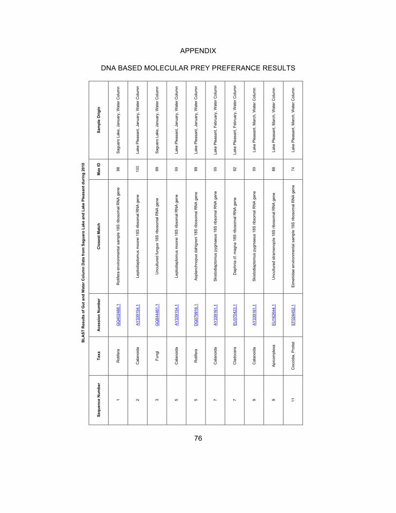
APPENDIX

DNA BASED MOLECULAR PREY PREFERANCE RESULTS

Sam

ple

Orig

in

Sag

uaro

Lak

e, J

anua

ry, W

ater

Col

umn

Lake

Ple

asan

t, Ja

nuar

y, W

ater

Col

umn

Sag

uaro

Lak

e, J

anua

ry, W

ater

Col

umn

Lake

Ple

asan

t, Ja

nuar

y, W

ater

Col

umn

Lake

Ple

asan

t, Ja

nuar

y, W

ater

Col

umn

Lake

Ple

asan

t, Fe

brua

ry, W

ater

Col

umn

Lake

Ple

asan

t, Fe

brua

ry, W

ater

Col

umn

Lake

Ple

asan

t, M

arch

, Wat

er C

olum

n

Lake

Ple

asan

t, M

arch

, Wat

er C

olum

n

Lake

Ple

asan

t, M

arch

, Wat

er C

olum

n

Max

ID

98

100

99

99

99

99

92

99

88

74

Clo

sest

Mat

ch

Rot

ifera

env

ironm

enta

l sam

ple

18S

ribo

som

al R

NA

gen

e

Lept

odia

ptom

us m

oore

i 18S

ribs

omal

RN

A g

ene

Unc

ultu

red

fung

us 1

8S ri

boso

mal

RN

A g

ene

Lept

odia

ptom

us m

oore

i 18S

ribs

omal

RN

A g

ene

Asp

lanc

hnop

us d

ahlg

reni

18S

ribo

som

al R

NA

gen

e

Ski

stod

iapt

omus

pyg

mae

us 1

8S ri

bsom

al R

NA

gen

e

Dap

hnia

cf.

mag

na 1

8S ri

boso

mal

RN

A g

ene

Ski

stod

iapt

omus

pyg

mae

us 1

8S ri

bsom

al R

NA

gen

e

Unc

ultu

red

stra

men

opile

18S

ribo

som

al R

NA

gen

e

Eim

eriid

ae e

nviro

nmen

tal s

ampl

e 18

S ri

boso

mal

RN

A g

ene

Ace

ssio

n N

umbe

r

GQ

4024

86.1

AY

3391

54.1

GQ

8444

61.1

AY

3391

54.1

DQ

0799

16.1

AY

3391

61.1

EU

3704

23.1

AY

3391

61.1

EU

1626

44.1

EF0

2445

2.1

Taxa

Rot

ifera

Cal

anoi

da

Fung

i

Cal

anoi

da

Rot

ifera

Cal

anoi

da

Cla

doce

ra

Cal

anoi

da

Api

com

plex

a

Coc

cidi

a, P

rotis

t BLA

ST R

esul

ts o

f Gut

and

Wat

er C

olum

n D

ata

from

Sag

uaro

Lak

e an

d La

ke P

leas

ant d

urin

g 20

10

Sequ

ence

Num

ber

1 2 3 5 5 7 7 9 9 11

76

Lake

Ple

asan

t, M

arch

, Wat

er C

olum

n

Lake

Ple

asan

t, M

arch

, Wat

er C

olum

n

Lake

Ple

asan

t, M

arch

, Wat

er C

olum

n

Lake

Ple

asan

t, M

arch

, Wat

er C

olum

n

Lake

Ple

asan

t, M

arch

, Wat

er C

olum

n

Lake

Ple

asan

t, M

arch

, Wat

er C

olum

n

Sag

uaro

Lak

e, A

pril,

Wat

er C

olum

n

Sag

uaro

Lak

e, A

pril,

Wat

er C

olum

n

Sag

uaro

Lak

e, A

pril,

Wat

er C

olum

n

Sag

uaro

Lak

e, A

pril,

Wat

er C

olum

n

Sag

uaro

Lak

e, A

pril,

Wat

er C

olum

n

Lake

Ple

asan

t, A

pril,

Wat

er C

olum

n

99

69

99

95

99

89

97

77

92

98

84

98

Ski

stod

iapt

omus

pyg

mae

us 1

8S ri

bsom

al R

NA

gen

e

Trip

artic

alca

r sp.

18S

ribo

som

al R

NA

gen

e

Lept

odia

ptom

us m

oore

i 18S

ribs

omal

RN

A g

ene

Unc

ultu

red

cilia

te 1

8S ri

boso

mal

RN

A g

ene

Lept

odia

ptom

us m

oore

i 18S

ribs

omal

RN

A g

ene

Unc

ultu

red

Chl

orop

hyta

18S

ribo

som

al R

NA

gen

e

Unc

ultu

red

euka

ryot

ic p

icop

lank

ton

18S

ribo

som

al R

NA

gen

e

Unc

ultu

red

cilia

te 1

8S ri

boso

mal

RN

A g

ene

Unc

ultu

red

cilia

te 1

8S ri

boso

mal

RN

A g

ene

Plo

esom

a hu

dson

i 18S

ribo

som

al R

NA

gen

e

Chl

amyd

omon

as re

inha

rdtii

gen

e fo

r 18S

rRN

A

Ski

stod

iapt

omus

pyg

mae

us

AY

3391

61.1

FJ82

7659

.1

AY

3391

54.1

FJ93

9037

.1

AY

3391

54.1

HQ

2193

99.1

AY

6426

98.1

HQ

2193

69.1

EU

1438

73.1

DQ

2977

14.1

AB

5118

37.1

AY

3391

61.1

Cal

anoi

da

Fung

i

Cal

anoi

da

Cili

opho

ra

Cal

anoi

da

Chl

orop

hyta

Cili

opho

ra

Cili

opho

ra

Cili

opho

ra

Rot

ifera

Chl

orop

hyta

Cal

anoi

da

13

11

13

13

15

15

17

19

21

22

23

25

77

Lake

Ple

asan

t, A

pril,

Wat

er C

olum

n

Lake

Ple

asan

t, A

pril,

Wat

er C

olum

n

Lake

Ple

asan

t, A

pril,

Wat

er C

olum

n

Sag

uaro

Lak

e, M

ay, C

yclo

poid

Lake

Ple

asan

t, A

pril,

Wat

er C

olum

n

Sag

uaro

Lak

e, M

ay, C

yclo

poid

Sag

uaro

Lak

e, M

ay, C

yclo

poid

Sag

uaro

Lak

e, M

ay, D

aphn

ia

Sag

uaro

Lak

e, M

ay, N

aupl

ii

Sag

uaro

Lak

e, M

ay, N

aupl

ii

Lake

Ple

asan

t, Ju

ne, C

alan

oid

Lake

Ple

asan

t, Ju

ne, C

alan

oid

92

92

99

87

87

96

97

97

97

97

99

100

Unc

ultu

red

Chl

orop

hyta

18S

ribo

som

al R

NA

gen

e

Unc

ultu

red

alve

olat

e 18

S rR

NA

gen

e

Ski

stod

iapt

omus

pyg

mae

us

Tetra

selm

is k

ochi

ensi

s

Unc

ultu

red

euka

ryot

e 18

S ri

boso

mal

RN

A g

ene

Unc

ultu

red

mar

ine

euka

ryot

e 18

S ri

boso

mal

RN

A g

ene

Unc

ultu

red

alve

olat

e 18

S ri

boso

mal

RN

A g

ene

Unc

ultu

red

euka

ryot

ic p

icop

lank

ton

18S

ribo

som

al R

NA

gen

e

Unc

ultu

red

alve

olat

e pa

rtial

18S

rRN

A g

ene

Unc

ultu

red

fresh

wat

er e

ukar

yote

18S

ribo

som

al R

NA

gen

e

Ski

stod

iapt

omus

pyg

mae

us 1

8S ri

bsom

al R

NA

gen

e

Ski

stod

iapt

omus

pyg

mae

us 1

8S ri

bsom

al R

NA

gen

e

HQ

2193

99.1

FN69

0047

.1

AY

3391

61.1

AJ4

3137

0.2

EU

3509

18.1

AY

3317

81.2

FJ93

9051

.1

AY

6426

98.1

FN69

0357

.1

HM

1381

67.1

AY

3391

61.1

AY

3391

61.1

Chl

orop

hyta

Cili

opho

ra

Cal

anoi

da

Chl

orop

hyta

Din

ophy

ceae

Cili

opho

ra

Cili

opho

ra

Cili

opho

ra

Cili

opho

ra

Cili

opho

ra

Cal

anoi

da

Cal

anoi

da

27

25

27

29

27

29

31

35

37

39

43

45

78

Lake

Ple

asan

t, Ju

ne, C

yclo

poid

Lake

Ple

asan

t, Ju

ne, C

yclo

poid

Sag

uaro

Lak

e, J

une,

Cyc

lopo

id

Sag

uaro

Lak

e, J

une,

Nau

plii

Lake

Ple

asan

t, Ju

ly, W

ater

Col

umn

Lake

Ple

asan

t, Ju

ly, W

ater

Col

umn

Lake

Ple

asan

t, Ju

ly, W

ater

Col

umn

Lake

Ple

asan

t, Ju

ly, W

ater

Col

umn

Lake

Ple

asan

t, Ju

ly, W

ater

Col

umn

Lake

Ple

asan

t, Ju

ly, C

alan

oid

Lake

Ple

asan

t, Ju

ly, C

alan

oid

Lake

Ple

asan

t, Ju

ly, N

aupl

ii

84

83

84

94

78

91

70

93

80

99

99

71

Opi

stho

nect

a m

inim

a 18

S ri

boso

mal

RN

A g

ene

Ski

stod

iapt

omus

pyg

mae

us 1

8S ri

bsom

al R

NA

gen

e

Unc

ultu

red

alve

olat

e 18

S ri

boso

mal

RN

A g

ene

Unc

ultu

red

alve

olat

e 18

S ri

boso

mal

RN

A g

ene

Unc

ultu

red

Ban

isve

ld e

ukar

yote

18S

ribo

som

al R

NA

gen

e

Unc

ultu

red

euka

ryot

e 18

S ri

boso

mal

RN

A g

ene

Unc

ultu

red

euka

ryot

ic p

icop

lank

ton

18S

ribo

som

al R

NA

gen

e

Unc

ultu

red

euka

ryot

e 18

S ri

boso

mal

RN

A g

ene

Orp

inom

yces

sp.

Lept

odia

ptom

us m

oore

i 18S

ribs

omal

RN

A g

ene

Lept

odia

ptom

us m

oore

i 18S

ribs

omal

RN

A g

ene

Scl

erau

loph

orus

cep

hala

tus

18S

ribo

som

al R

NA

gen

e

EF4

1783

4.1

AY

3391

61.1

FJ41

0727

.1

FJ41

0727

.1

EU

0918

55.1

DQ

6747

68.1

DQ

4091

10.1

DQ

6747

68.1

AJ8

6464

9.1

AY

3391

54.1

AY

3391

54.1

AF1

6742

3.1

Cili

opho

ra

Cal

anoi

da

Din

ophy

ceae

Din

ophy

ceae

Api

com

plex

a

Kin

etop

last

ida

Spi

zello

myc

etal

es

Spe

rmat

ophy

ta

Fung

i

Cal

anoi

da

Cal

anoi

da

Pro

pora

ta

47

49

51

53

55

57

59

61

63

65

67

69

79

Lake

Ple

asan

t, A

ugus

t, W

ater

Col

umn

Lake

Ple

asan

t, A

ugus

t, W

ater

Col

umn

Lake

Ple

asan

t, A

ugus

t, W

ater

Col

umn

Lake

Ple

asan

t, A

ugus

t, W

ater

Col

umn

Lake

Ple

asan

t, A

ugus

t, W

ater

Col

umn

Lake

Ple

asan

t, A

ugus

t, W

ater

Col

umn

Lake

Ple

asan

t, A

ugus

t, W

ater

Col

umn

Lake

Ple

asan

t, A

ugus

t, W

ater

Col

umn

Lake

Ple

asan

t, A

ugus

t, W

ater

Col

umn

Lake

Ple

asan

t, A

ugus

t, W

ater

Col

umn

Lake

Ple

asan

t, A

ugus

t, C

yclo

poid

Lake

Ple

asan

t, A

ugus

t, C

yclo

poid

95

83

92

84

89

87

89

96

90

96

80

78

Unc

ultu

red

euka

ryot

ic p

icop

lank

ton

18S

ribo

som

al R

NA

gen

e

Unc

ultu

red

mar

ine

euka

ryot

e 18

S ri

boso

mal

RN

A

Mes

ochy

trium

pen

etra

ns

Bos

min

a lo

ngiro

stris

Test

udin

ella

sp.

18S

ribo

som

al R

NA

gen

e

Unc

ultu

red

euka

ryot

e 18

S ri

boso

mal

RN

A g

ene

Vor

ticel

la g

raci

lis 1

8S ri

boso

mal

RN

A g

ene

Din

ofla

gella

te 1

8S ri

boso

mal

RN

A g

ene

Mac

roch

aetu

s co

llins

i 18S

ribo

som

al R

NA

gen

e

Unc

ultu

red

euka

ryot

e 18

S ri

boso

mal

RN

A g

ene

Het

eroc

apsa

triq

uetra

Filin

ia lo

ngis

eta

18S

ribo

som

al R

NA

gen

e

EF1

9677

2.1

DQ

2481

92.1

FJ80

4149

.1

AM

4902

75.1

AY

2181

13.1

EU

1440

03.1

GQ

8724

29.1

AY

4605

74.1

DQ

2977

05.1

GU

2901

01.1

AJ4

1551

4.1

DQ

0799

14.1

Rhi

zidi

omyc

etac

eae

Bic

osoe

cida

e

Fung

i

Bos

min

a

Rot

ifera

Din

ophy

ceae

Cili

opho

ra

Din

ophy

ceae

Rot

ifera

Cod

onos

igid

ae

Din

ophy

ceae

Rot

ifera

71

73

76

78

75

77

79

81

81

83

85

85

80

Lake

Ple

asan

t, A

ugus

t, C

yclo

poid

Lake

Ple

asan

t, A

ugus

t, D

aphn

ia

Lake

Ple

asan

t, A

ugus

t, D

aphn

ia

Lake

Ple

asan

t, A

ugus

t, N

aupl

ii

Sag

uaro

Lak

e, A

ugus

t, W

ater

Col

umn

Sag

uaro

Lak

e, A

ugus

t, W

ater

Col

umn

Sag

uaro

Lak

e, A

ugus

t, W

ater

Col

umn

Sag

uaro

Lak

e, A

ugus

t, W

ater

Col

umn

Sag

uaro

Lak

e, A

ugus

t, W

ater

Col

umn

Sag

uaro

Lak

e, A

ugus

t, W

ater

Col

umn

Sag

uaro

Lak

e, A

ugus

t, W

ater

Col

umn

Sag

uaro

Lak

e, A

ugus

t, W

ater

Col

umn

97

69

99

99

72

97

67

99

91

97

96

94

Test

udin

ella

sp.

18S

ribo

som

al R

NA

gen

e

Unc

ultu

red

euka

ryot

e ge

ne fo

r SS

U rR

NA

Dap

hnia

cf.

mag

na B

MR

-200

8

Mon

omm

ata

mac

ulat

a 18

S ri

boso

mal

RN

A g

ene

Ano

phyr

oide

s ha

emop

hila

18S

ribo

som

al R

NA

gen

e

Unc

ultu

red

euka

ryot

e 18

S ri

boso

mal

RN

A g

ene

Tric

hoce

rca

elon

gata

18S

ribo

som

al R

NA

gen

e

Unc

ultu

red

cilia

te 1

8S ri

boso

mal

RN

A g

ene

Unc

ultu

red

alve

olat

e 18

S ri

boso

mal

RN

A g

ene

Unc

ultu

red

alve

olat

e pa

rtial

18S

rRN

A g

ene

Unc

ultu

red

mon

ogon

onta

n pa

rtial

18S

rRN

A g

ene

Unc

ultu

red

cilia

te 1

8S ri

boso

mal

RN

A g

ene

AY

2181

13.1

AB

2750

16.1

EU

3704

23.1

DQ

2977

07.1

U51

554.

1

HM

2275

12.1

DQ

2977

21.1

FJ93

9037

.1

GQ

8444

27.1

FN69

0042

.1

AM

1798

18.1

FJ76

5378

.1

Rot

ifera

Cya

nidi

ales

Dap

hnia

Rot

ifera

Cili

opho

ra

Icht

hyos

pore

a

Cili

opho

ra

Cili

opho

ra

Cili

opho

ra

Cili

opho

ra

Rot

ifera

Cili

opho

ra

87

89

91

91

95

99

101

103

98

100

104

100

81

Sag

uaro

Lak

e, A

ugus

t, N

aupl

ii

Sag

uaro

Lak

e, A

ugus

t, W

ater

Col

umn

Sag

uaro

Lak

e, A

ugus

t, W

ater

Col

umn

Sag

uaro

Lak

e, A

ugus

t, N

aupl

ii

Sag

uaro

Lak

e, A

ugus

t, W

ater

Col

umn

Sag

uaro

Lak

e, A

ugus

t, N

aupl

ii

Sag

uaro

Lak

e, A

ugus

t, N

aupl

ii

Sag

uaro

Lak

e, A

ugus

t, N

aupl

ii

Sag

uaro

Lak

e, A

ugus

t, N

aupl

ii

Sag

uaro

Lak

e, A

ugus

t, N

aupl

ii

Sag

uaro

Lak

e, A

ugus

t, N

aupl

ii

Sag

uaro

Lak

e, A

ugus

t, N

aupl

ii

79

78

98

96%

90

97

94

90

88

99

90

99

Pty

gura

libe

ra 1

8S ri

boso

mal

RN

A g

ene

Pte

rocy

stis

folia

cea

18S

ribo

som

al R

NA

gen

e

Unc

ultu

red

cilia

te 1

8S ri

boso

mal

RN

A g

ene

Tric

hoce

rca

rattu

s 18

S ri

boso

mal

RN

A g

ene

Sca

ridiu

m lo

ngic

audu

m 1

8S ri

boso

mal

RN

A g

ene

Unc

ultu

red

alve

olat

e 18

S rR

NA

gen

e

Unc

ultu

red

mon

ogon

onta

n 18

S rR

NA

gen

e

Pla

tyop

hrya

vor

ax 1

8S ri

boso

mal

RN

A g

ene

Unc

ultu

red

euka

ryot

e 18

S ri

boso

mal

RN

A g

ene

Not

omm

ata

cord

onel

la

Pla

tyop

hrya

vor

ax 1

8S ri

boso

mal

RN

A g

ene

Vor

ticel

la g

raci

lis 1

8S ri

boso

mal

RN

A g

ene

DQ

2976

89.1

AY

7495

99.1

HQ

2194

32.1

DQ

2977

22.1

DQ

2977

20.1

FN69

0046

.1

AM

1798

18.1

AF0

6045

4.1

EU

8604

96.1

DQ

2977

11.1

AF0

6045

4.1

GQ

8724

29.1

Cili

opho

ra

Aca

ntho

cyst

idae

Cili

opho

ra

Cili

opho

ra

Rot

ifera

Cili

opho

ra

Rot

ifera

Cili

opho

ra

Cili

opho

ra

Rot

ifera

Cili

opho

ra

Cili

opho

ra

106

102

104

106

104

106

108

106

108

110

108

110

82

Sag

uaro

Lak

e, A

ugus

t, N

aupl

ii

Lake

Ple

asan

t, S

epte

mbe

r, W

ater

Col

umn

Lake

Ple

asan

t, S

epte

mbe

r, W

ater

Col

umn

Lake

Ple

asan

t, S

epte

mbe

r, W

ater

Col

umn

Lake

Ple

asan

t, S

epte

mbe

r, W

ater

Col

umn

Lake

Ple

asan

t, S

epte

mbe

r, W

ater

Col

umn

Lake

Ple

asan

t, S

epte

mbe

r, W

ater

Col

umn

Lake

Ple

asan

t, S

epte

mbe

r, W

ater

Col

umn

Lake

Ple

asan

t, S

epte

mbe

r, W

ater

Col

umn

Lake

Ple

asan

t, S

epte

mbe

r, W

ater

Col

umn

Lake

Ple

asan

t, S

epte

mbe

r, D

iaph

anos

oma

Lake

Ple

asan

t, S

epte

mbe

r, D

iaph

anos

oma

99

99

97

85

98

96

87

80

97

92

92

92

Pol

yarth

ra re

mat

a 18

S ri

boso

mal

RN

A g

ene

Pol

yarth

ra re

mat

a

Unc

ultu

red

fung

us 1

8S ri

boso

mal

RN

A g

ene

Unc

ultu

red

cilia

te 1

8S ri

boso

mal

RN

A g

ene

Unc

ultu

red

cilia

te 1

8S ri

boso

mal

RN

A g

ene

Unc

ultu

red

alve

olat

e 18

S rR

NA

gen

e

Unc

ultu

red

cilia

te 1

8S ri

boso

mal

RN

A g

ene

Unc

ultu

red

Rim

ostro

mbi

dium

18S

ribo

som

al R

NA

gen

e

Unc

ultu

red

fresh

wat

er e

ukar

yote

18S

ribo

som

al R

NA

gen

e

Unc

ultu

red

dino

flage

llate

18S

ribo

som

al R

NA

gen

e

Dia

phan

osom

a sp

. TS

-199

9 18

S ri

boso

mal

RN

A g

ene

Dia

phan

osom

a sp

. TS

-199

9 18

S ri

boso

mal

RN

A g

ene

DQ

2977

16.1

DQ

2977

16.1

GU

0679

82.1

GU

0679

75.1

FJ41

0586

.1

FN69

0357

.1

EU

1438

58.1

GU

0678

19.1

FJ76

5408

.1

HQ

1913

24.1

AF1

4421

0.1

AF1

4421

0.1

Rot

ifera

Rot

ifera

Fung

us

Cili

opho

ra

Cili

opho

ra

Cili

opho

ra

Cili

opho

ra

Cili

opho

ra

Cili

opho

ra

Din

ophy

ceae

Dia

phan

osom

a

Dia

phan

osom

a

110

116

114

116

116

118

118

120

120

122

124

126

83

Lake

Ple

asan

t, S

epte

mbe

r, C

alan

oid

Lake

Ple

asan

t, S

epte

mbe

r, C

alan

oid

Lake

Ple

asan

t, S

epte

mbe

r, C

alan

oid

Lake

Ple

asan

t, S

epte

mbe

r, B

osm

ina

Lake

Ple

asan

t, S

epte

mbe

r, B

osm

ina

Sag

uaro

Lak

e, S

epte

mbe

r, W

ater

Col

umn

Sag

uaro

Lak

e, S

epte

mbe

r, W

ater

Col

umn

Sag

uaro

Lak

e, S

epte

mbe

r, W

ater

Col

umn

Sag

uaro

Lak

e, S

epte

mbe

r, W

ater

Col

umn

Sag

uaro

Lak

e, S

epte

mbe

r, W

ater

Col

umn

Sag

uaro

Lak

e, S

epte

mbe

r, W

ater

Col

umn

Sag

uaro

Lak

e, S

epte

mbe

r, W

ater

Col

umn

94

100

100

91

72

96

83

72

89

90

77

75

Stro

mbi

dium

cf.

basi

mor

phum

Lept

odia

ptom

us m

oore

i 18S

ribs

omal

RN

A g

ene

Ski

stod

iapt

omus

pyg

mae

us 1

8S ri

bsom

al R

NA

gen

e

Cili

ate

sp. N

CM

S06

01

Unc

ultu

red

euka

ryot

e 18

S ri

boso

mal

RN

A g

ene

Mes

eres

cor

lissi

stra

in C

HI

Nol

andi

a sp

. WY

G07

0507

02

Stro

bilid

ium

sp.

clo

ne S

trob0

0ssu

_1

Pel

agot

hrix

alv

eola

ta

Cili

ate

sp. N

CM

S06

0

Cili

ate

sp. N

CM

S06

01

Nol

andi

a sp

. WY

G07

0507

02

FJ48

0419

.1

AY

3391

54.1

AY

3391

61.1

AM

4125

25.1

GU

4744

06.1

EU

3995

29.1

FJ85

8215

.1

AF3

9912

4.1

AB

4860

09.1

AM

4125

25.1

AM

4125

25.1

FJ85

8215

.1

Cili

opho

ra

Cal

anoi

da

Cal

anoi

da

Cili

opho

ra

Bos

min

a

Cili

opho

ra

Cili

opho

ra

Cili

opho

ra

Cili

opho

ra

Cili

opho

ra

Cili

opho

ra

Cili

opho

ra

128

128

130

132

132

134

134

136

136

138

138

140

84

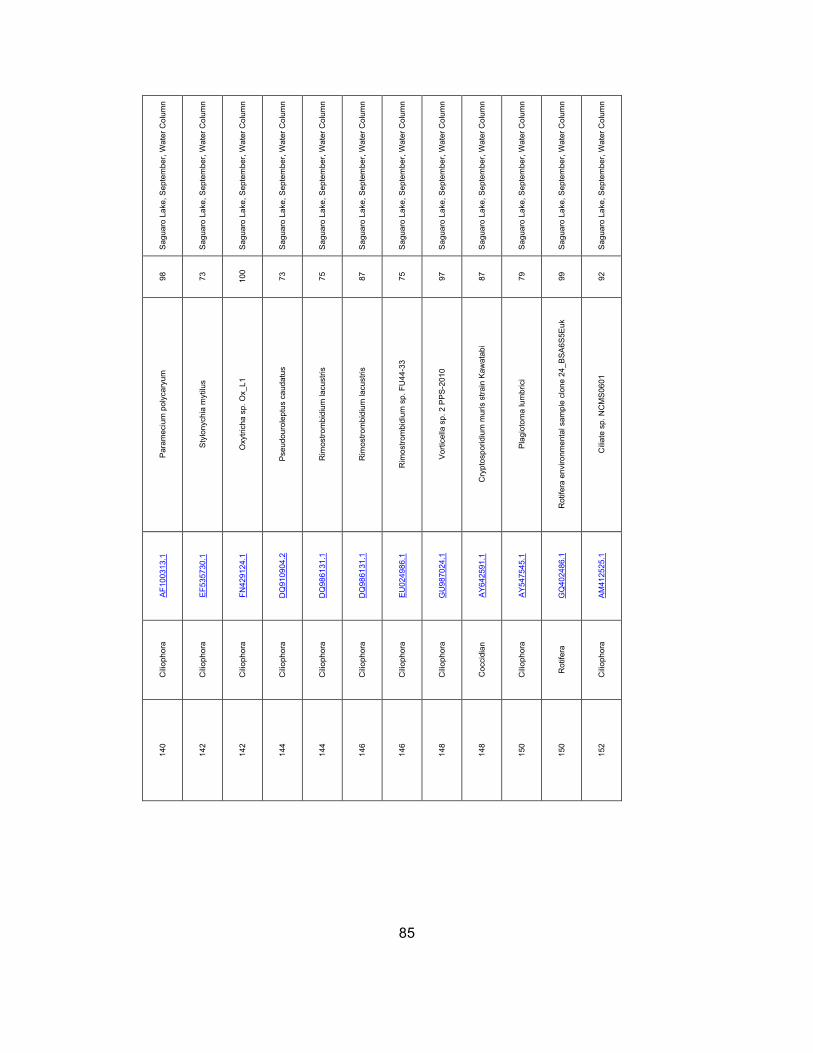
Sag

uaro

Lak

e, S

epte

mbe

r, W

ater

Col

umn

Sag

uaro

Lak

e, S

epte

mbe

r, W

ater

Col

umn

Sag

uaro

Lak

e, S

epte

mbe

r, W

ater

Col

umn

Sag

uaro

Lak

e, S

epte

mbe

r, W

ater

Col

umn

Sag

uaro

Lak

e, S

epte

mbe

r, W

ater

Col

umn

Sag

uaro

Lak

e, S

epte

mbe

r, W

ater

Col

umn

Sag

uaro

Lak

e, S

epte

mbe

r, W

ater

Col

umn

Sag

uaro

Lak

e, S

epte

mbe

r, W

ater

Col

umn

Sag

uaro

Lak

e, S

epte

mbe

r, W

ater

Col

umn

Sag

uaro

Lak

e, S

epte

mbe

r, W

ater

Col

umn

Sag

uaro

Lak

e, S

epte

mbe

r, W

ater

Col

umn

Sag

uaro

Lak

e, S

epte

mbe

r, W

ater

Col

umn

98

73

100

73

75

87

75

97

87

79

99

92

Par

amec

ium

pol

ycar

yum

Sty

lony

chia

myt

ilus

Oxy

trich

a sp

. Ox_

L1

Pse

udou

role

ptus

cau

datu

s

Rim

ostro

mbi

dium

lacu

stris

Rim

ostro

mbi

dium

lacu

stris

Rim

ostro

mbi

dium

sp.

FU

44-3

3

Vor

ticel

la s

p. 2

PP

S-2

010

Cry

ptos

porid

ium

mur

is s

train

Kaw

atab

i

Pla

giot

oma

lum

bric

i

Rot

ifera

env

ironm

enta

l sam

ple

clon

e 24

_BS

A6S

5Euk

Cili

ate

sp. N

CM

S06

01

AF1

0031

3.1

EF5

3573

0.1

FN42

9124

.1

DQ

9109

04.2

DQ

9861

31.1

DQ

9861

31.1

EU

0249

86.1

GU

9870

24.1

AY

6425

91.1

AY

5475

45.1

GQ

4024

86.1

AM

4125

25.1

Cili

opho

ra

Cili

opho

ra

Cili

opho

ra

Cili

opho

ra

Cili

opho

ra

Cili

opho

ra

Cili

opho

ra

Cili

opho

ra

Coc

cidi

an

Cili

opho

ra

Rot

ifera

Cili

opho

ra

140

142

142

144

144

146

146

148

148

150

150

152

85

Sag

uaro

Lak

e, S

epte

mbe

r, W

ater

Col

umn

Sag

uaro

Lak

e, S

epte

mbe

r, W

ater

Col

umn

Sag

uaro

Lak

e, S

epte

mbe

r, W

ater

Col

umn

Sag

uaro

Lak

e, S

epte

mbe

r, N

aupl

ii

Sag

uaro

Lak

e, S

epte

mbe

r, N

aupl

ii

Sag

uaro

Lak

e, S

epte

mbe

r, N

aupl

ii

Sag

uaro

Lak

e, S

epte

mbe

r, N

aupl

ii

Lake

Ple

asan

t, O

ctob

er, W

ater

Col

umn

Lake

Ple

asan

t, O

ctob

er, W

ater

Col

umn

Lake

Ple

asan

t, O

ctob

er, W

ater

Col

umn

Lake

Ple

asan

t, O

ctob

er, W

ater

Col

umn

Lake

Ple

asan

t, O

ctob

er, W

ater

Col

umn

97

89

99

95

98

99

98

89

73

77

80%

98%

Plo

esom

a hu

dson

i

Par

astro

mbi

dino

psis

min

ima

Asp

lanc

hnop

us d

ahlg

reni

Nov

istro

mbi

dium

orie

ntal

e

Pro

ales

dol

iaris

Rot

ifera

env

ironm

enta

l sam

ple

clon

e 24

_BS

A6S

5Euk

Not

omm

ata

alla

ntoi

s

Stra

men

opile

sp.

MA

ST-

12 K

KTS

_D3

Mor

tiere

lla s

p. C

O-2

1

Rhi

zoph

ydiu

m s

p. J

EL3

17 is

olat

e A

FTO

L-ID

35

Pow

ello

myc

es s

p. J

EL9

5

Stro

mbi

diid

ae s

p. L

O12

8-19

DQ

2977

14.1

DQ

3937

86.1

DQ

0799

16.1

FJ42

2988

.1

DQ

2977

17.1

GQ

4024

86.1

DQ

2977

10.1

EF2

1938

1.1

AB

5210

52.1

AY

6358

21.1

AF1

6424

5.2

EU

0249

94.1

Rot

ifera

Cili

opho

ra

Rot

ifera

Cili

opho

ra

Rot

ifera

Rot

ifera

Rot

ifera

Dia

tom

Fung

i

Fung

i

Fung

i

Cili

opho

ra

152

154

154

156

158

160

162

166

168

170

172

174

86

Lake

Ple

asan

t, O

ctob

er, W

ater

Col

umn

Lake

Ple

asan

t, O

ctob

er, W

ater

Col

umn

Lake

Ple

asan

t, O

ctob

er, W

ater

Col

umn

Lake

Ple

asan

t, O

ctob

er, N

aupl

ii

Sag

uaro

Lak

e, O

ctob

er, W

ater

Col

umn

Sag

uaro

Lak

e, O

ctob

er, W

ater

Col

umn

Sag

uaro

Lak

e, O

ctob

er, W

ater

Col

umn

Sag

uaro

Lak

e, O

ctob

er, W

ater

Col

umn

Sag

uaro

Lak

e, O

ctob

er, N

aupl

ii

Lake

Ple

asan

t, N

ovem

ber,

Wat

er C

olum

n

Lake

Ple

asan

t, N

ovem

ber,

Wat

er C

olum

n

Lake

Ple

asan

t, N

ovem

ber,

Wat

er C

olum

n

72%

93%

100%

100%

84%

88%

90%

74%

99%

91

98

83

Chr

ysoc

hrom

ulin

a pa

rva

Ski

stod

iapt

omus

pyg

mae

us

Ski

stod

iapt

omus

pyg

mae

us

Lept

odia

ptom

us m

oore

i

Nol

andi

a sp

. WY

G07

0507

02

Nol

andi

a sp

. WY

G07

0507

02

Par

astro

mbi

dino

psis

min

ima

Chr

ysoc

hrom

ulin

a pa

rva

Ker

atel

la q

uadr

ata

Cili

ate

sp. N

CM

S06

01

Cili

ate

sp. N

CM

S06

01

Icht

hyos

pore

a sp

. ATC

C P

RA

-279

AM

4910

19.1

AY

3391

61.1

AY

3391

61.1

AY

3391

54.1

FJ85

8215

.1

FJ85

8215

.1

DQ

3937

86.1

AM

4910

19.1

DQ

2976

97.1

AM

4125

25.1

AM

4125

25.1

GU

8101

44.1

Pry

mne

siac

eae

Cal

anoi

da

Cal

anoi

da

Cal

anoi

da

Cili

opho

ra

Cili

opho

ra

Cili

opho

ra

Pry

mne

siac

eae

Rot

ifera

Cili

opho

ra

Cili

opho

ra

Pro

tist

176

178

180

182

184

186

188

190

192

194

195

196

87

Lake

Ple

asan

t, N

ovem

ber,

Wat

er C

olum

n

Lake

Ple

asan

t, N

ovem

ber,

Wat

er C

olum

n

Lake

Ple

asan

t, N

ovem

ber,

Wat

er C

olum

n

Lake

Ple

asan

t, N

ovem

ber,

Wat

er C

olum

n

Lake

Ple

asan

t, N

ovem

ber,

Wat

er C

olum

n

Lake

Ple

asan

t, N

ovem

ber,

Wat

er C

olum

n

Lake

Ple

asan

t, N

ovem

ber,

Wat

er C

olum

n

Lake

Ple

asan

t, N

ovem

ber,

Wat

er C

olum

n

Lake

Ple

asan

t, N

ovem

ber,

Wat

er C

olum

n

Lake

Ple

asan

t, N

ovem

ber,

Wat

er C

olum

n

Lake

Ple

asan

t, N

ovem

ber,

Wat

er C

olum

n

Lake

Ple

asan

t, N

ovem

ber,

Wat

er C

olum

n

99

87

85

94

86

73

83

82

87

76

96

99

Cili

ate

sp. N

CM

S06

01

Bic

osoe

ca p

etio

lata

stra

in A

TCC

506

39

Cer

com

onad

ida

envi

ronm

enta

l sam

ple

N.v

itelli

na

Sap

role

gnia

sp.

SA

P4

Can

dida

kru

isii

Asp

idis

ca s

tein

i

Sph

aera

stru

m fo

ckii

18S

ribo

som

al R

NA

gen

E

Chi

lodo

nella

unc

inat

a cl

one

1

Vor

ticel

la s

p. S

P-2

009-

3

Vor

ticel

la c

ampa

nula

Lept

odia

ptom

us m

oore

i

AM

4125

25.1

AY

5204

44.1

EF0

2416

3.1

Z273

93.1

FJ79

4911

.1

AB

0135

43.1

AF3

0562

5.1

AY

7496

14.1

AF3

0028

1.1

GU

1870

50.1

AF3

3551

8.1

AY

3391

54.1

Cili

opho

ra

stra

men

opile

s

Rhi

zaria

Fung

us

stra

men

opile

s

Fung

us

Cili

opho

ra

Trem

atod

a, fl

uke

Cili

opho

ra

Cili

opho

ra

Cili

opho

ra

Cal

anoi

da

197

198

199

200

202

201

202

204

203

204

205

206

88

Lake

Ple

asan

t, N

ovem

ber,

Cyc

lopo

id

Lake

Ple

asan

t, N

ovem

ber,

Cyc

lopo

id

Lake

Ple

asan

t, N

ovem

ber,

Cyc

lopo

id

Sag

uaro

Lak

e, N

ovem

ber,

Wat

er C

olum

n

Sag

uaro

Lak

e, N

ovem

ber,

Wat

er C

olum

n

Sag

uaro

Lak

e, N

ovem

ber,

Wat

er C

olum

n

Sag

uaro

Lak

e, N

ovem

ber,

Wat

er C

olum

n

Sag

uaro

Lak

e, N

ovem

ber,

Wat

er C

olum

n

Sag

uaro

Lak

e, N

ovem

ber,

Wat

er C

olum

n

Sag

uaro

Lak

e, N

ovem

ber,

Wat

er C

olum

n

Sag

uaro

Lak

e, N

ovem

ber,

Cyc

lopo

id

Sag

uaro

Lak

e, N

ovem

ber,

Nau

plii

94

98

100

77

68

98

98

72

88

82

90

99

Icht

hyos

pore

a sp

. ATC

C P

RA

-280

Ski

stod

iapt

omus

pyg

mae

us

Lept

odia

ptom

us m

oore

i

Mor

tiere

lla m

ultid

ivar

icat

a

Cili

ate

sp. N

CM

S06

01

Spa

thid

ium

sta

mm

eri

Spa

thid

ium

sta

mm

eri

Pro

tasp

is o

bliq

ua is

olat

e 2

Par

astro

mbi

dino

psis

min

ima

Thec

ate

dino

flage

llate

UD

TSW

0701

Icht

hyos

pore

a sp

. ATC

C P

RA

-280

Col

loth

eca

cam

panu

lata

GU

8101

45.1

AY

3391

61.1

AY

3391

54.1

AF1

5714

4.1

AM

4125

25.1

DQ

4118

62.1

DQ

4118

62.1

FJ82

4122

.1

DQ

3937

86.1

AM

5039

29.1

GU

8101

45.1

DQ

2976

86.1

Pro

tist

Cal

anoi

da

Cal

anoi

da

Fung

i

Cili

opho

ra

Cili

opho

ra

Cili

opho

ra

Cili

opho

ra

Cili

opho

ra

Din

ophy

ceae

Pro

tist

Rot

ifera

207

208

209

210

211

212

213

214

215

217

219

221

89

Sag

uaro

Lak

e, N

ovem

ber,

Nau

plii

Lake

Ple

asan

t, D

ecem

ber,

Wat

er C

olum

n

Lake

Ple

asan

t, D

ecem

ber,

Wat

er C

olum

n

Lake

Ple

asan

t, D

ecem

ber,

Wat

er C

olum

n

Lake

Ple

asan

t, D

ecem

ber,

Wat

er C

olum

n

Lake

Ple

asan

t, D

ecem

ber,

Wat

er C

olum

n

Lake

Ple

asan

t, D

ecem

ber,

Wat

er C

olum

n

Lake

Ple

asan

t, D

ecem

ber,

Wat

er C

olum

n

Lake

Ple

asan

t, D

ecem

ber,

Cal

anoi

d

Lake

Ple

asan

t, D

ecem

ber,

Cal

anoi

d

Lake

Ple

asan

t, D

ecem

ber,

Nau

plii

Sag

uaro

Lak

e, D

ecem

ber,

Wat

er C

olum

n

79

95

90

90

95

80

92

92

94

100

98

90

Col

loth

eca

cam

panu

lata

Cili

ate

sp. N

CM

S06

01

Cili

ate

sp. N

CM

S06

01

Cili

ate

sp. N

CM

S06

01

Oxy

trich

a lo

nga

Cod

onos

igid

ae e

nviro

nmen

tal s

ampl

e

Rim

ostro

mbi

dium

lacu

stris

Ran

a sp

heno

ceph

ala

path

ogen

MJY

-200

7

Icht

hyos

pore

a sp

. ATC

C P

RA

-280

Ski

stod

iapt

omus

pyg

mae

us

Lept

odia

ptom

us m

oore

i

Cili

ate

sp. N

CM

S06

01

DQ

2976

86.1

AM

4125

25.1

AM

4125

25.1

AM

4125

25.1

AF5

0876

3.1

EF0

2401

2.1

DQ

9861

31.1

EF6

7561

6.1

GU

8101

45.1

AY

3391

61.1

AY

3391

54.1

AM

4125

25.1

Rot

ifera

Cili

opho

ra

Cili

opho

ra

Cili

opho

ra

Cili

opho

ra

Cho

anof

lage

llida

Cili

opho

ra

Alv

eola

ta

Pro

tist

Cal

anoi

da

Cal

anoi

da

Cili

opho

ra

222

223

224

225

226

227

228

229

230

231

232

233

90

Sag

uaro

Lak

e, D

ecem

ber,

Wat

er C

olum

n

Sag

uaro

Lak

e, D

ecem

ber,

Wat

er C

olum

n

Sag

uaro

Lak

e, D

ecem

ber,

Wat

er C

olum

n

Sag

uaro

Lak

e, D

ecem

ber,

Cyc

lopo

id

Sag

uaro

Lak

e, D

ecem

ber,

Nau

plii

Sag

uaro

Lak

e, D

ecem

ber,

Nau

plii

Sag

uaro

Lak

e, D

ecem

ber,

Nau

plii

94

93

93

93

98

76

99

Cili

ate

sp. N

CM

S06

01

Cili

ate

sp. N

CM

S06

01

Cili

ate

sp. N

CM

S06

01

Cili

ate

sp. N

CM

S06

01

Not

omm

ata

alla

ntoi

s 18

S

Unc

ultu

red

euka

ryot

e 18

S ri

boso

mal

RN

A g

ene

Plo

esom

a hu

dson

i

AM

4125

25.1

AM

4125

25.1

AM

4125

25.1

AM

4125

25.1

DQ

2977

10.1

AY

7495

32.1

DQ

2977

14.1

Cili

opho

ra

Cili

opho

ra

Cili

opho

ra

Cili

opho

ra

Rot

ifera

Cen

trohe

liozo

a

Rot

ifera

234

235

236

237

239

241

240

91