the dynamics of synchronization and phase regulation · (abraham, marsden, and ratiu) a trajectory...

Abraham and Garfinkel, Sync Rev 4 of 1 2 / 2 1 / 0 3 1

The Dynamics of Synchronization and Phase Regulation

Ralph AbrahamDepartment of Mathematics

University of California, Santa Cruz

Alan GarfinkelDepartments of Medicine (Cardiology) and Physiological Science

University of California, Los Angeles

Dedicated to Arthur Winfree

Abstract

This is a joint project begun in 1983 and first reported in (Abraham, 1989). We were inspired by Arthur Winfree and have in mind a number of applications to medical physiology and mathemati-cal biology. The main theme is the role of the geometry of periodic attractors -- the shape of an attractive limit cycle and its isochrons -- in determining the phase synchrony of a network of het-erogeneous oscillators (periodic or chaotic). We present a profusely illustrated review of the geo-metric theory of the synchronization of periodic attractors, such as biological oscillators, by periodic pulsatile forcing. We think of this tutorial as “Winfree 101” but a number of new insights are included.

2

Contents (44 figs)

1. Introduction2. Favorite phase theory, analytical outline

2.1 The shape form2.2 Favorite phases2.3 The favorite phase formula

3. Phase resetting, a tutorial (15 figs)3.1. How to draw an isochron (8 figs) 3.2. How to draw the phase foliation (1 figs)3.3. The density of the phase foliation (2 figs)3.4. Single pulsatile forces and the exact PRC (4 figs)

4. Favorite phases (7 figs)4.1. The shape-force function and the instantaneous PRC (2 figs)4.2. Periodic pulsatile forcing and favorite phases (2 figs)4.3. Huyghens’ clocks (3 figs)

5. The concept of phase regulation (6 figs)5.1. Favorite phase bifurcation due to varying the direction of forcing (4 figs)5.2. Favorite phase bifurcation due to varying the strength of forcing (1 fig)5.3. Favorite phase bifurcation due to varying the duration of forcing (1 fig)5.4. Fast regulation with a train of pulses5.5. Phase regulation design principles

6. Applications to Hodgkin-Huxley neural networks (16 figs)6.1. One HH neuron forced by a square wave (10 figs)6.2. One HH neuron forced by another HH neuron (5 figs)6.3. Two HH neurons, mutually coupled (1 fig)

7. ConclusionReferences (Articles)References (Books)

3

1. Introduction

Some years ago we worked together on the microstructure of forced oscillators, while studying various biorhythms of mammalian physiology. While the global analysis behind our ideas was eventually published, the basic intuitions of our theory have been buried in our files until now. In this long but nontechnical tutorial, we present the essential geometry of synchronization and phase regulation of coupled oscillators. In future work we plan to carry out some physiological applica-tions in more detail.

2. Favorite phase theory, an analytical outline

A dynamical system is a vectorfield V assigning a velocity vector, V(p), to each point p of state space M, a differentiable manifold. (Abraham, Marsden, and Ratiu) A trajectory is a curve in M that is everywhere tangent to the vectorfield V. An oscillatory process is then modeled as a periodic attractor

Γ

of some dynamical system. We assume throughout that

Γ

is a periodic attractor, repre-senting a stable oscillation. (Hirsch and Smale)

We consider now a periodic perturbation of

Γ.

Thus we embed V in a dynamical scheme, that is, a family of vectorfields, V

c

, where c belongs to a parameter space, C, called the control space. We have another dynamical system, the forcing system, with vectorfield U and state space L. Finally, we have a coupling function, f: L

�

C. The periodically forced system then is a vectorfield, U x V, on the product manifold, L x M. For simplicity, we assume the L is a one-dimensional torus, or cir-

cle, S

1

, and U is a constant speed of 1, so L is a periodic attractor of period 2

π

. This is the situation usually expressed by the first order autonomous system of ordinary differential equations,

θ

’ = 1x’ = V(x) + W(

θ

)

or equivalently, by the time-dependent system,

x’ = V(x) + f(t)

where f is a periodic, vector valued, function. (Abraham and Shaw) This latter form is also useful if we wish to consider the effect of a single short pulsatile force.

Now if V is the forced process, and W is a perturbing wave representing the driving force, how will W change the oscillation

Γ

? Consider the state point going around the unperturbed limit cycle

Γ

. The effect of W is to lift the state point briefly off

Γ

. Then the dynamics of the governing vector field, V, will return the state point back to

Γ

, but it will typically be to a different point on

Γ

than if it had not been perturbed. We say the perturbation has reset the phase of

Γ

.

In order to determine how the phase has been reset, we begin with the assumption that in a small neighborhood of

Γ

, it has isochrons; that is, through every point on

Γ

there is a unique arc that intersects

Γ

cleanly and such that every point on that arc will return to the same phase of

Γ

. This is a consequence of hyperbolicity, a generic property of smooth vectorfields. (Abraham and Robbin; Hirsch, Pugh, and Shub) Isochrons were introduced by Winfree in his work on phase resetting

4

curves. (Winfree, 1980, p. 82; 1987, p. 54.) Isochrons provide the geometric basis for phase reset-ting curves, or PRCs. We now review the geometric theory of phase resetting.

2.1. The shape form

The contribution made by the shape of

Γ

can be made precise. First, we decompose T

p

(M), the tan-gent space to M at a point p, into a one-dimensional subspace tangent to

Γ

(denoted = <V

p

>, the space spanned by the vector V

p

) and its complement I

p

(tangent to the isochron at p)

T

p

(M) = <V

p

> + I

p

In general, I

p

is the generalized eigenspace of the attractive eigenvalues of the periodic flow. That is, it is tangent to the isochrons of

Γ

within the unperturbed vectorfield, V. (Hirsch, Pugh, and Shub, 1977) Here it is one-dimensional.

We then use this decomposition to split the effect of an instantaneous perturbation into a compo-nent along V

p

that changes the phase, and a component within I

p

that has no effect on phase, that is, it perturbs within an isochron. Thus if W

p

is the perturbation acting at p

ε

Γ

, then

W

p

= Z

p

+ Y

p

,

where Y

p

ε

I

p

and

Z

p

ε

<V

p

>. Since the component that changes the phase, Z

p

, belongs to the one-dimensional space <V

p

>, there is a scalar

α

ε

R such that,

Z

p

=

α

p

V

p.

In this way, we can assign a real number

α

p

to each W

p

, and that defines a function from T

p

(M) to R, hence is a 1-form on T

p

(M). We call this the

shape form

of

Γ

,

α

(

p

)

. It depends on the shape of

Γ

, and the geometry of the underlying dynamical system, V. The

shape-force function

is the inner product of the shape form and a time-dependent forcing vectorfield. All these will be explained below.

2.2. Favorite phases

Suppose V is a vectorfield that is subjected to a small periodic perturbation, W. We can represent the perturbed vectorfield as V(x) + W(q, x), where W is periodic in q, and x

ε

M. Now suppose

Γ

is a periodic orbit that is an attractor of V. Choose a point p

0

ε Γ,

as a fiducial point for phase refer-ence. Then, assuming the perturbation is sufficiently small, the perturbed vectorfield has a periodic orbit

Γ

* that is also an attractor, and pierces the phase zero section

Σ

at a unique point p

0

*. (Abra-ham and Robbin) This point lies on a unique isochron of the original orbit

Γ

,

and we call this point the

relative phase

. The effect of a brief perturbation by W is a change from a phase of V on

Γ

to its relative phase under V+W, after W is withdrawn, and the system relaxes back to

Γ

. This effect is approximated by the component of W along

Γ

, that is, its value by the shape form of W on

Γ

, which projects along the isochrons of

Γ

. Let W/

Γ

denote this projected vectorfield on

Γ

. Its attrac-tors are the favorite phases of the W

/ Γ

system.

5

2.3. The favorite phase formula

We now introduce a formula for the favorite phases. Basically, the idea is that the favorite phases are the integrals of the action of the phase shift due to a perturbation at p

ε Γ, integrated over all p.

where δ(φ0) is the infinitesimal phase change at the fiducial phase φ0 , α is the shape form, and P is the periodic perturbation. The phase change is therefore the integral of the local phase shifts, inte-grated around the periodic perturbation. (Abraham, 1989; p. 71). All this will be illustrated below in a particular case.

3. Phase resetting, a tutorial Arthur Winfree, in his extensive work on circadian rhythms, put great emphasis on the phase reset-ting curve, or PRC, and phase singularities. In this section, we relate the isochrons, phase foliation, shape form, and favorite phases of the preceding section to these well-known features of Winfree’s geometry of time.

3.1. How to draw an isochron The isochron concept is easy enough to grasp, yet given the equations defining a dynamical system with a periodic attractor, how can we locate an isochron? We are now going to outline a simple computational approach, using a typical two-dimensional system as an example: the Rayleigh sys-tem with all coefficients set to one. (Abraham and Shaw, 1992, Exm 4a, p. 212) The steps could be accomplished with any number of available software packages: Matlab, Maple, Mathematica, Stella, or Berkeley Madonna, for example. We have used Berkeley Madonna for some of the fig-ures in this section. The equations of the system are,

x' = y

y' = -x-y3+y

The first step is to identify, roughly, a periodic attractor, or PA. As this system has only one attrac-tor, we need not seek out its basin boundary. (There is a point repellor at the origin, which does not belong to the basin of the PA.) Thus, any point in the two-dimensional state space may be taken as an initial point, and integration by the Euler method, for example, will reveal the PA accurately enough. A few more experiments will provide us with an approximate value for the period of the PA.

The isochron is mapped into itself by repeated applications of the map F which advances every point forward along its trajectory by the period of the PA. This is a discrete dynamical system within the isochron, and every point approaches the phase zero point of the PA asymptotically. They all share the same asymptotic phase, phase zero.

These steps are carried in Figures 3.1.1-8, in a simple case.

δ ϕ0( ) αptP ϕ t( ) td

Γ∫=

ξ


Fig. 3.1.1. Here is a rectangular open set in the basin of attraction of the unique periodic attractor of our system, x and y range from –4 to 4, and a single trajectory is shown, beginning from the initial point, (2, 2). It spirals clockwise, approaching rather quickly to the PA, asymptotically from the outside.

Fig. 3.1.2.We now choose any point on the PA, and call it the phase zero point. Here we have chosen the point p0 = (1.254416835, 0).

Fig. 3.1.3.We now measure the period of the PA by integrating from p0 until the trajectory passes again through (or within some small epsilon) of p0, and noting the time of this passage. The period of this PA is approximately τ = 6.6632.


Fig. 3.1.4.Let F denote the map that advances any point, say q0, τ time units (one period) for-ward along its trajectory, to q1. For example, the small disk A0 is mapped to the flattened blot A1 = F[A0].

Fig. 3.1.5.

Similarly, let F-1 denote the inverse map of F. This maps every point q0 t time units (one period) backward along its trajectory, to q-1. The small disk A0 is mapped to the elongated

blob, A-1 = F-1[A0]. The elongating aspect of this map is the secret to drawing an isochron.

Fig. 3.1.6.Through the point p0 we now draw a very short line segment, T(0), transversal (that is, not tangent) to the PA. We will choose a hor-izontal line segment.


Fig. 3.1.7.

Applying F-1 a few times, the short transver-sal is lengthened outside the PA, pulled towards infinity. This process converges, as the preimages of the transversal approach asymptotically to the isochron of phase zero, I0. Here is an enlargement of T(-1) in a small box at the point p0, made with extensive inte-grations by Berkeley Madonna.

Fig. 3.1.8.Inside the PA, the short transversal is pulled towards a repellor. This will turn out to be a singularity of the phase foliation, the famous phase singularity of Winfree. In this case, we have a counterclockwise spiral point repellor at the origin, but the isochrons spiral out clockwise from it.

The convergence of the pulling back process is very rapid in this case, so that T(-1) and T(-2) are nearly identical. This is due to two special conditions here: the attraction to the PA is very strong, and the initial transversal, T(0), is rather close to the isochron by happenstance. Thus the curve shown above, a segment of T(-1), approximates the phase zero isochron very closely.


3.2. How to draw the phase foliationNow, again following Winfree, lets divide the basin of the PA (that is, the entire state box, except-ing a small disk or point inside the PA) into six time zones. Of course there are infinitely many isochrons in the phase foliation, one for each phase, but these six time zones are enough to get the picture, as shown in Fig. 3.2.1. (See Hirsch, Shub, and Pugh on normal coordinates for proofs of all this.)

Push-forward methodParameterizing the dynamics by degrees of phase instead of time, advance every point of the zero phase isochron by 60 degrees (equivalent to τ/6 time units),. This gives us a segment of the 60 degree phase isochron, I60. Repeating this construction, we obtain the 120, 180, 240, and 300 degree phase isochrons. This construction of the phase foliation is conceptual, the successive images of a finite segment of the zero phase isochron grow shorter very rapidly.

Pull-back methodAfter we have drawn the PA and determined its period as above, we may proceed as follows. Inte-grate backwards from the phase zero point an integral number of periods (we might try three for a start). Mark a point on this trajectory corresponding to each single period, getting a sequence of points, p0, p-1, p-2, p-3,... all on the phase zero isochron. Now integrate forward from the earliest point, changing the color of the trajectory every 60 degrees. The colors then correspond to time zones. But a variant of this procedure will be a little easier in our case.

Trajectory methodIn our exemplary system, the Rayleigh oscillator, a little exploration with an integrator such as Berkeley Madonna shows that the attraction to the PA is rather fast. Trajectories beginning on the bounding box shoot toward the PA, approximating an isochron. Within about one period, they turn and slow down to follow around the PA. We therefore adopt the following strategy to bring the phase foliation into view as a pattern of six colored time zones, each corresponding to a 60-degree interval of isochrons. We will simply color the first segment of a few trajectories beginning on the

Fig. 3.2.1Using an integrator, compute the trajectory from p0 from t = 0 to t = 6.66, one period. Looking at the table of values of (t, x(t), y(t)), select the values for each sixth of a period, t = 0, 1.1, 2.2, 3.3, 4.4, and 5.5. Plot these points on a graphic of the PA, and color by hand the arcs of the PA between these points. Using Winfree’s favorite color code, these are (from phase zero): red, yellow, green, cyan, blue, and magenta.

10

bounding box.

Now our task is to color the entire state rectangle with these six colors, identifying the six time zones corresponding to phases in the 60-degree phase intervals by these colors. The boundaries of the color zones will then indicate six isochrons of the phase foliation. We will proceed with this task “by hand,” although the procedure could easily be automated.

Imagine a thin rectangle, the target, about two timesteps wide around the point p0 = (1.25442, 0). If we are integrating with timestep 0.001 then we will be looking for values of y(t) in the window (-0.001, +0.001), corresponding to about one degree of phase. The height of the target may be made much larger, as the dynamic vector, V(p0), is approximately vertical, so x is changing relatively slowly near p0. We will check for x in the interval (1.24, 1.27).

Outer trajectoriesNext we will examine trajectories outside of the PA. Later we should also explore the inside of the PA, looking for the phase singularity. We will consider one-at-a-time a number of initial points on the bounding box of the state rectangle, beginning near the top left corner. So we take (-3, 4) as the initial point, and integrate for one period. (In our case this will suffice. But with other systems, one might need to integrate for two or more periods.) Viewing the table of values of (t, x(t), y(t)), we search down from the top as the values of y(t) decrease from 4 until the first negative value. Then we check to see if the value of x(t) is within the target. (In this case it is, otherwise we would keep searching down, and after one or more periods, we finally would find the trajectory within the tar-get. In our case, we find the two successive rows in the table of values,

3.786, 1.26257, -0.0001466853.787, 1.26257, +0.00111637

From these we may interpolate and round, concluding that at about t = 3.786, our trajectory start-ing near the upper left corner arrived very close to the phase zero isochron. Note that this is less than one period, 6.664. (If not, we would subtract an integral number of periods to find a remain-der.) We now want to move backwards along the trajectory from phase zero, coloring it mentally for each sixth of a period (about 1.11) with its appropriate time zone code color. These are (round-ing):

(2.68, 3.79) magenta(1.57, 2.68) blue(0.46, 1.57) cyan(0.00, 0.46) green

As we stop our mental coloring process on reaching back to the initial point, we will call this green segment, t in (0,00, 0.46), the initial zone segment of the trajectory from (-3, 4). This is about half of a 60-degree time zone. The other three color-coded segments (cyan, blue, and magenta) all cross a full time zone.

Carrying out this method for several trajectories gives an impression of the phase foliation, as

11

shown in Fig. 3.2.2.

3.3. The density of the phase foliationWe should now make a careful note of the relationship between the geometry and the phase density of isochrons in the phase foliation. In case the velocity vector V(p) at a point p in the PA is large, the isochrons corresponding to two successive phases (say, one degree apart) will have relatively more geometric space between them. In the Rayleigh system pictured here, the speed — the length of the (x’, y’) vector — has a spike of about 1.65 shortly before phases zero and 180 degrees, and a minimum of about 0.9 before 90 and 270 degrees.

3.4. Single pulsatile forces and the exact PRCGiven a PA and its phase foliation, we consider now a single, strong, and very short perturbation by an external force. We say force because the Rayleigh system is a second order system,the first equation says that x’ = y, meaning that x is the displacement of something, and y is its velocity. Therefore, y’ = x” = a, the acceleration, and if the system derives from Newton’s law, F = ma, then a is proportional to the force, F. In any case, we imagine the short perturbation to be a vectorfield – large, uniform, and pointing straight up – which as added to the vectorfield V during a very brief interval of time: a single, brief pulsatile force. We are now going to illustrate one of the key concepts of Arthur Winfree, the phase resetting curve, or PRC.

We may generalize the construction by considering the single application of an external force of a larger magnitude, and/or a longer duration. In fact, Winfree considered the strength of the perturba-tion to be determined either by the height of the force, or its duration, or both. For example, the brightness and duration of a pulse of white light, resetting the phase of a lattice of fruit flies. In any case, a unique PRC is defined by the experimental procedure outlined here, applied to any given PA and phase foliation.

Fig. 3.2.2Here are the color coded trajectories for eight initial points on the boundary of the rectangular box. The phase foliation outside the PA may be estimated from these visual data.


-180 +180

+10

-10

Fig. 3.4.1Here we show a trajectory along the PA (black), suddenly jerked upwards (red) by an instantaneous upward force. After the cessa-tion of that brief force, the perturbed point continues along a new trajectory of the origi-nal system (blue).

Fig. 3.4.2Here we superimpose on the hook (perturba-tion) shown above, a piece of the isochron (green) passing through the endpoint of the hook. This shows us the asymptotic phase of the blue trajectory, retarded significantly from the phase of the unperturbed (black) trajectory (yellow isochron). This phase dif-ference, negative in this case, is the phase resetting due to this single pulsatile force.

Fig. 3.4.4.Repeating this construction for a large num-ber of points along the PA creates this curve, the phase resetting curve or PRC. The curve depends of course on the original vectorfield V, through its phase foliation, and the per-turbing force amplitude and duration. Here we plot relative (new) phase resetting versus old phase. (Compare Winfree, 1987; p. 54.)

Fig. 3.4.3.Here we repeat the preceding construction, but to the left of (earlier in time than) a favorite phase. That is, the phase reset is pos-itive (advance) rather than negative (retard). See that the yellow isochron (unforced sys-tem) precedes the green isochron (forced system).

13

4. Favorite phasesWe now zoom in to a closer look at the phase resetting process, in the case of a relatively brief pulsatile force.

4.1. The shape-force function and the instantaneous PRC Note that the phase resetting by a pulsatile force applied near p, as shown in Fig. 3.4.2, involves primarily the PA component. To first approximation, the isochronal components of F produce per-turbations (hooks) with the same final isochron, and thus, the same phase resetting. To predict the phase reset by a single pulse of the vector F, we need consider only its PA-tangential component, which is fully specified by its value under the shape form at p, as shown in Fig. 4.1.1.

Now we consider the case of a constant perturbing force vectorfield, F, applied at every point in the basin of the PA. We carry out the construction above for every point p of the PA. We obtain then a real-valued function, a(F), defined on the PA. If we now parameterize the PA by phases (in degrees) we may represent this function, which depends vitally on the phase foliation and the con-stant force F, by a graph. This function may be regarded as the instantaneous PRC, as it approxi-mates the phase resetting by a pulse of force F and duration ∆t, for small ∆t. The graph appears very similar to the PRC graph shown in Fig. 3.4.3. However, we may also visualize the vectors Fv(p) for all p in the PA as a vectorfield on the PA. We may call this the phase resetting vector-field, or PRV, shown in Fig. 4.2.2.


F F

Fi

v

p

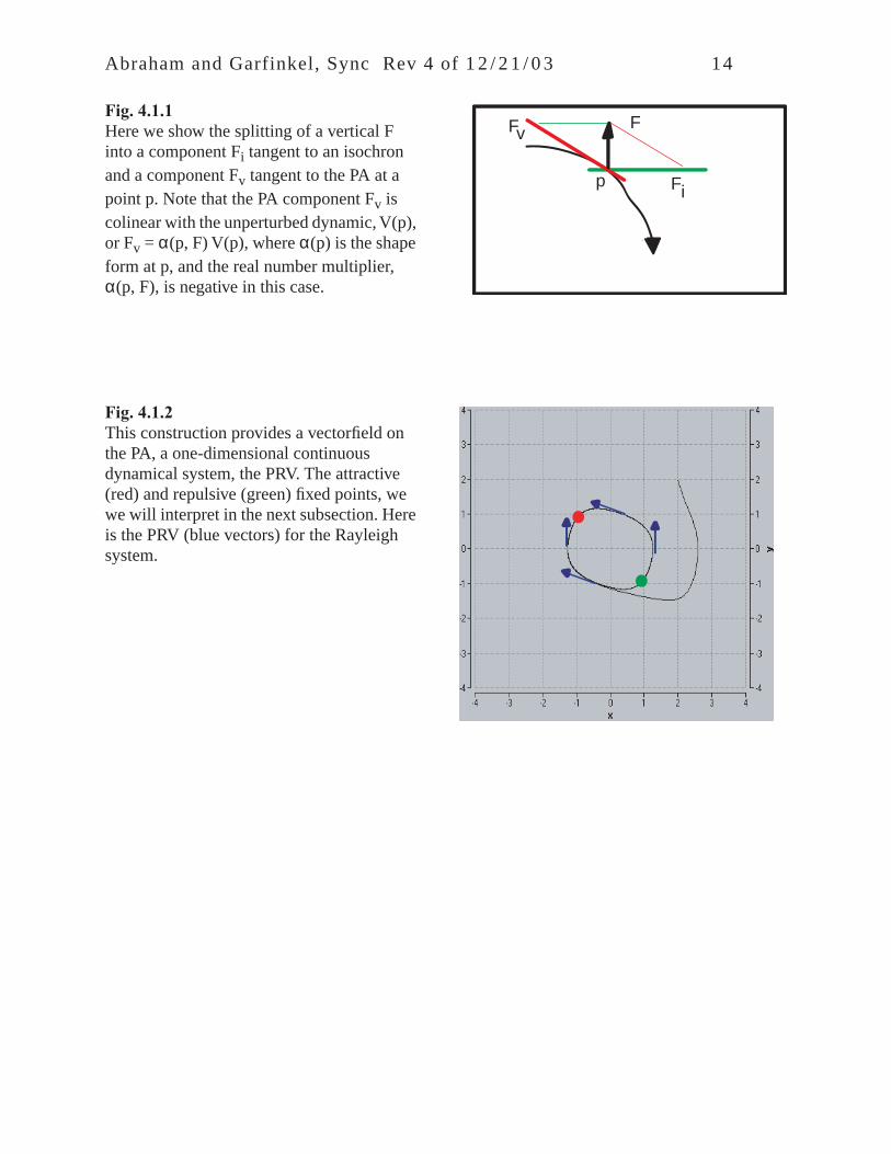
Fig. 4.1.1Here we show the splitting of a vertical F into a component Fi tangent to an isochron and a component Fv tangent to the PA at a point p. Note that the PA component Fv is colinear with the unperturbed dynamic, V(p), or Fv = α(p, F) V(p), where α(p) is the shape form at p, and the real number multiplier, α(p, F), is negative in this case.

Fig. 4.1.2This construction provides a vectorfield on the PA, a one-dimensional continuous dynamical system, the PRV. The attractive (red) and repulsive (green) fixed points, we we will interpret in the next subsection. Here is the PRV (blue vectors) for the Rayleigh system.

15

123

4.2. Periodic pulsatile forces and favorite phasesWe now consider a most important situation: a pulsatile external force is applied as above, not just once, but periodically. Further, we consider only the case in which the system having one PA is forced periodically and synchronously. That is, a pulse is applied after the passage of each unit of time exactly equal to the period of the unforced PA.

The proper dynamical system defined by a periodically forced planar system is a three-dimen-sional ring, as described in “A short course in toral arrangement” (Abraham and Shaw, 1992). Here however, we will continue with the two-dimensional representation introduced above for a single pulsatile perturbation – the upswinging red hook of Section 3.4. After one hook, we will suppose that the blue trajectory relaxes to the unperturbed PA in much less than one period. Thus the next perturbation will arrive at a phase following (or preceding) the first hook by a phase dif-ference given by the PRC, hence a second hook will be seen to the right (or sometimes to the left) of the first hook. And so on, as shown here. As we might have predicted on the basis of theory, these hooks converge on an attractive fixed point of the PRC, regarded as a one-dimensional dis-crete dynamical system – a favorite phase. See Fig. 4.2.1.

Note that the blue snap-back of a hook is eventually in phase with the green isochron passing through the upper end of the red part of the hook. Thus, we may imagine that the system snaps-back instantaneously along the green isochron, rather than rapidly along the blue trajectory.

In other words, the effect of a pulse of duration Dt is to move the trajectory cycling around the PA from its phase when the pulse begins, to the reset phase when the pulse ends. The unperturbed system would have moved forward along the PA, according to the speed of the PA (inverse to its period). If the duration, Dt, is small relative to the speed, 360/tau degrees per second say, then the forward motion of the unperturbed system during the duration of the pulse will be insignificant.

Fig. 4.2.1Here we show three hooks from a sequence of hooks converging to a favorite phase of the Rayleigh system. At 1 the trajectory hooks upward (red) during a pulse, zooms downward (blue) close to an isochron after the pulse. The step backwards along the PA from the beginning of the red to the end of the blue is the loss of phase due to the pulse. At 2, the phase loss is shorter, as the forward motion (red hook) during the pulse (same time duration) is slower here. At 3, the favor-ite, the red hook covers the blue: no phase is lost.

16

Let us assume so.

Note also, in Figure 4.2.1, that the heights of the three hooks are all about the same. This is because the durations of the pulses are assumed to be the same, and the amplitude of the vertical force, F, is constant. Meanwhile, the widths of the three hooks are declining, because the angles between F and the isochrons are decreasing, thus also the tangential component of F, as shown in Figure 4.1.1.

Then if a periodic sequence of identical pulses is given with the same period as (that is, synchro-nously with) this PA, then each red hook will depart the PA almost exactly where the preceding green snap-back landed. This situation is shown in Figure 4.2.2. By the way, this figure appears in the final preprint of Hayashi’s career, and as far as we know, has never been published. (Hayashi, 1984) From the preprint, it appears that Hayashi was inspired in this work by receiving a preprint from Vassalo-Pereira, in 1981. We are grateful to Hayashi for sending a copy of his preprint in 1984, which first alerted us to the work of Vassalo-Pereira, and inspired our earlier paper. (Abra-ham, 1989)

4.3 Huyghens’ clocksWe go on now to an important example of phase regulation, which will lead us into the next sec-tion, on desirable characteristics of entrainers and entrainees. This is the famous example of Chris-

Fig. 4.2.2.This figure by Chihiro Hayashi shows (in mono-chrome) the actual trajectory of a synchronously forced PA of a system similar to our example, the Rayleigh system. Here, the PA is circular. (Hayashi, 1984)

17

tian Huyghens of February, 1665. This example, and its sequel literature, have inspired our favorite phase formula. (Abraham, 1989). This phenomenon of phase entrainment should not be confused with frequency entrainment, in which the two clocks would have the same frequency, but the phase difference of their pendulums would be arbitrary.

Writing to his father in 1665, Christiaan Huyghens noted that two clocks hanging on the same wall displayed “sympathie,” in which their pendulums came to swing phase-locked, that is, with a con-stant phase difference of 180 degrees, regardless of their original phases. (Bleckhman, p. 147; Abraham and Shaw; Pikovsky; Strogatz)

Translations from the Latin of the correspondence of Huyghens on his experiments is given in full in (Pikovsky, 2001), and a nice narrative in (Strogatz, 2003). The dynamical model for Huyghens' clocks is treated in much detail in (Andronov, Khaiken, Witt, 1959/1963; p. 168). The analysis of the Andronov model that inspired our study of pulsatile periodic forcing described above is found in (Vassalo-Pereira, 1989). The phase entrainment of clocks had not received a satisfactory treat-ment until this work of Vassalo-Pereira. His account can be cast naturally in the language of phase regulation. As our model of the clock, we follow Vassalo-Pereira’s account of the clock model of Andronov.

We consider here a single-pulse escapement, following Vassalo-Pereira. Andronov also gives a double-pulse model, which fits better with Huyghens' reports. The single-pulse model gives a boost to the pendulum only once during its full cycle, and synchrony occurs only at a single favor-

Fig. 4.3.1.Here we have the two-hook (tick-tock) model of Andronov. (Andronov, 1959) The PA (here marked limit cycle) progresses clockwise with two jumps.

18

ite phase, the zero phase.

Now let us consider the effect of an energy pulse on this system. In Huyghens’ example, this pulse will come from the “tock” of the escapement mechanism (the energy supply) of the other clock, transmitted as a solitary wave passing through the wall (the coupling medium). Such a transfer of energy would take the form of an energy pulse, that is, an instantaneous change in V, since, in Newtonian mechanics, forces produce accelerations, that is, changes in V. We assume that this energy pulse looks like a rectangle.

If an external, periodic, synchronous, pulsatile force is applied to this system, the phase resets will converge to a favorite phase at the tock. Similarly, if a downward periodic force were applied, the

Fig. 4.3.2The (piecewise smooth) periodic attractor consists of two semicircles. In the lower half plane, a semi-circle centered at the point I = (+ beta, 0). In the upper half plane, segments of two semicircles cen-tered at the point II = (- beta, 0). The radii are such that the semicircles meet at two points on the hori-zontal axis. The vertical straight line segment cor-responds to the periodic single-pulse (tock) force applied by the escapement mechanism. This draw-ing by Timothy Poston (Abraham, 1989) is based on (Vassalo-Pereira, 1982).

Fig. 4.3.3The isochrons of this model are straight lines radiat-ing from I into the lower half-plane, and from II into the upper half plane. This figure, also copied from (Vassalo-Pereira, 1982; p. 348) by Timothy Poston, (Abraham, 1989) is an example of a radial isochron clock (RIC), like many biological clocks. (Hoppens-taedt, Keener, 1982)

19

12

6

favorite phase would be found at the bottom of the PA.

5. The concept of phase regulationHayashi (1984), influenced by Vassalo-Pereira (1981), was an early advocate of the phase regula-tion idea. In this section we illustrate this concept with three examples of favorite phase bifurca-tion: those due to variation of the direction of the external force, to the amplitude of the force, and finally, to the width of the pulse. In each case the forced system is a two-dimensional PA with radial isochrons, an RIC.

5.1. Favorite phase bifurcation due to varying the direction of forcingWe consider an external force applied in synchronous, periodic, pulses, to a given RIC. Keeping the amplitude and pulse width of the force small and fixed, we will vary its direction stepwise in a circle, clockwise around the face of a fictitious clock. We will now carry out this thought experi-ment with a few different RICs, beginning with the circular one considered by Hayashi.

Figure 5.1.1.Here the RIC is a clockwise circle, with a uniform speed. When the external force, F, is upwards (pointing to the 12) the favorite phase is also at the 12, As we vary the direc-tion of F to the 1, the 2, and so on, the favor-ite phase just follows along.

20

12

3

6

9

12

3

6

9

12

3

6

9

Figure 5.1.2.We now repeat the experiment with this RIC. It has a sharp hump at the top, like some camels. As F rotates clockwise from the 12, the favorite phase follows, but not uniform-ily. It hovers near the 12 until F approaches the 3. Likewise if F rotates counterclockwise from the 12, the favorite phase hovers near the 12 until F approaches the 9. We regard this as a sort of stability for the favorite phase at 12.

Figure 5.1.3.Now here is a new wrinkle! This PA has two humps like some other camels. If we begin a sequence of up-pointing sync-periodic pulses when the system is moving near the 3, we find convergence to the hump at the 1. But if we begin the sequence when the sys-tem is near the 9, we find convergence to the hump at 11. There are two favorite phases for up-pointing forcing, and two basins of attrac-tion. And if F is rotated, interesting bifurca-tions occur.

Figure 5.1.4In fact, with this three-humped camel, rota-tion of F clockwise from the 12 back to the 12 exhibits double-fold catastrophes thrice. This type of PA shape is actually found in nature, or at least in some nature-imitating models, such as the Brusselator, and the Hodgkin-Huxley neuron.

21

12

3

6

9

5.2. Favorite phase bifurcation due to varying the strength of forcingThe behavior of the favorite phase configuration under variation of the amplitude of F, with direc-tion and pulse width held constant, depends very much on the geometry of the phase foliation. We may imagine geometries in catastrophic bifurcations occur, even though we may not be able to find exemplary systems exhibiting these geometries. One such imaginary portrait is shown in Fig. 5.2.1.

Figure 5.2.1.Here is an ordinary garden-variety PA pos-sessing a weird and kinky phase foliation. Two hooks are shown, both for a narrow pulse of an up-pointing force. But one is weak, and the other strong. Note that the weak hook behaves like Fig. 3.4.2, but the strong hook reaches an isochron that goes around the barn before docking on the PA. This is another catastrophic bifurcation in the favorite phase portrait.

5.3. Favorite phase bifurcation due to varying the duration of forcingFinally, we hold direction and amplitude of sync-periodic forcing fixed, and vary the pulse width only. At this point we need to consider the integral formula from Sec. 2.3. We simply consider a single fat pulse as the sum of consecutive thin pulses. If they all agree which way to go (that is, the whole fat pulse is in the basin of a single favorite phase) then they behave just as the thin pulses considered above. However, what if they disagree?

Figure 5.3.1.Here again our two-humped camel. But here we have a fat pulse draped over the entire camel’s back: there is only one favorite phase for this big boy.


5.4. Fast regulation with a train of pulsesIn the case of subharmonic periodic forcing (e.g., every other cycle of the PA is forced by an exter-nal pulse) the phase resets accumulate to a favorite phase as in the harmonic case, although perhaps more slowly. But in the case of fast, superharmonic, periodic forcing, the cumulative effect of a train of pulses occupying an interval of time is much like the effect of a single isolated wide pulse occu-pying the same interval of time. If the train precedes a favorite phase, the cumulative effect is an advance of phase toward the favorite phase, Similarly, it the pulse train follows the favorite phase, the effect will be a retard, again towards the favorite phase. But if the pulse train is draped over the favorite phase, with some pulses preceding and others following, the phase shifts might balance. This situation is similar to the wide balancing pulse shown in the preceding figure.

5.5. Phase regulation design principlesWe may now summarize the intuitions we have gained on favorite phases and phase regulation with two design principles for forced oscillator engineers.

5.5.1. Good entrainersGiven an entrainee (a fixed PA of a dynamical system) and having chosen a direction for synchro-nous external forcing, we should examine the phase foliation and favorite phases of the PA. In case there is more than one favorite phase, the forcing pulse should be thin relative to the basin of the desired favorite phase. The amplitude may be high if the isochrons are not too radically curved.

5.5.2. Good entraineesGiven an entrainee and a given direction of external periodic forcing, we must consider again the phase foliation and favorite phase-force dynamic on the chosen PA. The curvature of the PA near the desired favorite phase should be adequate to guarantee some stability of the favorite phase under perturbation of the direction, amplitude, and width of the forcing pulse.

Our geometric theory applies, but our visualization strategy does not. The isochrons are 3-dimen-sional hypersurfaces, but we may still view the perturbed trajectories projected into a plane. WE have chosen the (n, v) plane for this purpose.

23

6. Applications to Hodgkin-Huxley neural networksIn this section we will apply our ideas on phase regulation to small complex systems composed of coupled HH neurons. In three subsections, we consider one HH neuron forced by a rectangular pulse, one HH forced by another HH, and two HH neurons, mutually coupled.

6.1. One Hodgkin-Huxley neuron forced by a square waveThe HH model is a four-dimensional dynamical system with a robust periodic attractor. The state space is euclidean four-space, and the coordinate variables (including the ranges and the colors we use in the graphics) are:

h, activation for closure of Na gate, black, range 0 to 0.45m, activation for opening of Na gate, red, range 0 to 1.00n, activation for opening of K gate, green, range 0.4 to 0.75v, voltage, red, range -80 to +30

With our typical values for the various parameters, the period of this oscillation is 12.89 time units. Each cycle provides a fast pulse of voltage from resting (ca minus 74) to peak (ca 20 volts).

Our geometric theory applies, but our visualization strategy does not. The isochrons are 3-dimen-sional hypersurfaces, but we may still view the perturbed trajectories projected into a plane. We have chosen the (n, v) plane for this purpose.


Fig. 6.1.1. [hh001.gif]No forcing. Here we see the time series of v and n for a single period of the PA, 12.89 units of time.

Fig. 6.1.1a. [hh001a.gif]Same values as above, projected into the (n, v) plane. The initial point is the black dot, and the tra-jectory moves clockwise around the cycle.


Fig 6.1.2. [hh001.gif, 150 dpi]Perturbed with a single pulse of amplitude 100 and duration 10 degrees,in the v direction, beginning at phase 30 degrees. Note that the forcing pulse, magenta, approxi-mates the voltage pulse of the HH system, as for example, applied by a neighboring neuron.

Fig. 6.1.2a. [hh002a.gif, 150 dpi]Plane projection of Figure 6.2. Note that the phase reset is negative here, as the cycle ends some-what short of the full cycle of the unperturbed system, Figure 6.1a. Examination of the table of val-ues of the two integrations shows this retard to be about 9 degrees. Here we show the red hook (upward forcing during the pulse) and the blue swoop (relaxing transient after the pulse). The green dot shows where the isochron at the end of the red hook meets the PA, 9 degrees before the begin-ning of the red hook.


Fig. 6.1.3. [hh003a.gif, 150 dpi]Here we have integrated for two cycles of the forced system. The hook of the second forcing pulse appears here to the right of the first hook, due to the 9 degrees of phase retard.

Fig. 6.1.4. [hh004a.gif, 150 dpi]Similarly, here we show 10 cycles of the forced system. Convergence to a favorite phase on the right side of the PA is suggested. This is our first Hayashi plot. The first pulse begins a the bottom of the voltage cycle, which we call zero degrees of phase of the forced system.


Fig. 6.1.5. [hh005a.gif, 150 dpi]And here, carried to extremes, 100 cycles, and we have found a favorite phase.

Fig. 6.1.6. [hh006a.gif, 150 dpi]We now try a single pulse beginning at 90 degrees phase of the forced system, just after the begin-ning of the rapid rise in voltage. Notice the slight bump at the lower left of the loop.


Fig. 6.1.7. [hh007a.gif, 150 dpi]Periodic repetition of the pulse of Figure 6.1.6 for 100 cycles yields this portrait, showing conver-gence from the left to the same favorite phase indicated in Figure 6.5. This is our second Hayashi plot for the periodically forced HH system. The two Hayashi plots show that there is a single favorite phase, shortly after the maximum rise of the voltage, as our geometric theory would pre-dict, for the upward vertical pulsatile force.

29

Fig. 6.1.8. [hh018a.gif, 150 dpi]And here are two cycles of the forcing square wave, 10 degrees wide, (D, black) along with the voltage (v, red) versus TIME, after 1000 cycles. Here we clearly see the attachment of the forcing pulse to the favorite phase of the HH system, about 9 degrees after the peak of the forced voltage at top dead center. This run began with the forcing pulse at 90 degrees of phase of the forced sys-tem. Exactly the same figure is obtained when beginning at 0 degrees of phase, as indicated by the two Hayashi plots.


6.2. One HH neuron forced by another HH neuronIn the preceding subsection we have forced an HH with a rectangular pulse that approximates an HH pulse, but, with floor zero. That is, the dv/dt equation has been forced with a periodic rectan-gular pulse of period 12.89 (360 degrees), floor zero, ceiling 100, and width 0.358 (10 degrees). The initial phase lag is immaterial, as convergence to the favorite phase difference is quickly established.

We now replace this periodic pulsatile forcing by an HH neuron model identical to the forced sys-tem. Again, the initial phase lag is irrelevant, and here we have used phase lag zero. That is, the two HH systems are begun in unison, at the minimum of voltage, and integrated for 100 periods, as in Figures 6.1.5 and 6.1.7. This time we view the asymptotic behavior by plotting the time series for v1 (the forced HH voltage) and v2 (the forcing voltage) against time, for the time inter-val [1200, 1300], that is, from period 93 to 100. Note: (v2 + 74) is used as the forcing signal.

Fig. 6.2.1. [hh5.gif, 150 dpi]In green we see seven cycles of the forcing HH voltage, and in blue, the forced HH voltage, after about 100 cycles. As in the case of the rectangular pulsatile forcing of the same frequency and size, the asymptotic phase difference again places the peak of the forcing pulse about a tenth of a cycle after the peak of the forced neuron. In fact, smaller and slightly larger phase lags alternate. Also, note that the blue plot shows a slow subharmonic or chaotic disturbance, probably due to the wide skirt of the forcing HH pulse, relative to the forcing rectangular pulse of the preceding sub-section. The situation is the same after 1000 cycles.


Figure 6.2.2. [hh009a.gif, 150 dpi]Here we show v1 (voltage of the forced HH neuron) versus v2 (the forcer). At the gap (upper cen-ter of figure) the higher point is the initial condition, and the motion is CCW. Here we show only cycles 100 to 110, that is, after the transient has settled to the attractor.

Figure 6.2.3. [hh010b.gif, 150 dpi]This is a new view of the same run as above. Here we show v1' vs v1,. Again we see what appears to be a Rossler-type of chaotic attractor.


Figure 6.2.4. [fig hh012a.gif, 150 dpi]Compare this with Figure 6.2.1. Here we have reduced the strength of the forcing of v1 by v2 to one half. Note that the subharmonic is much weaker here.

Figure 6.2.4. [fig hh012a.gif, 150 dpi]Compare this with Figure 6.2.1. Here we have reduced the strength of the forcing of v1 by v2 to one half. Note that the subharmonic or chaotic perturbation is much weaker here.

Figure 6.2.5. [fig hh013a.gif, 150 dpi]Compare this with Figures 6.2.1 and 6.2.4. Here we have reduced the strength of the forcing of v1 by v2 to one tenth. Note that the subharmonic or chaotic perturbation is very much weaker here.


6.3. Two HH neurons, mutually coupledWe next consider two HH neurons, each forced by the other. This means that to the equation

v1dot = function1 of (v1, h1, m1, n1)we add a term: gamma 21 times v2, and similarly, to the equation

v2dot = function2 of (v2, h2, m2, n2)we add a term: gamma12 times v1.

First we consider the symmetrical case, in which the two coupling constants (gamma21 and gamma 12) are equal, and equal to one tenth, as in the preceding figure. Here we get a wonderful yet intuitive result: perfect synchrony.

Figure 6.3.1. [hh014.gif, 150 dpi]The two traces, v1 (blue) and v2 (green) coincide exactly, after the decay of an initial transient. And the common behavior mimics that of the voltage of an unforced HH neuron.

If we now consider a gradual change of the two coupling constants from (0.1, 0.0) as in Figure 6.2.5, to (0.1, 0.1) as shown here, and then on to (0.0, 0.1) which would be shown by Figure 6.2.5 with the two colors reversed, we see that we may engineer the phase relation between the two neu-rons to be anywhere from -9 degrees to +9 degrees, just by adjusting the coupling constants.

This is highly suggestive, and is the source of our phrase, “phase regulation engineering” intro-duced some years ago. In fact, this suggests that biological evolution has selected for effective coupling strengths in the biological brain, heart and so on, just as artificial neural networks are trained by Hebbian learning rules.

34

7. ConclusionAnd so we have now illustrated the main geometrical features of our theory of phase regulation. And in the context of the Hodgkin-Huxley neuron model, we have shown them in a physiological context. Along the way, we have seen that the favorite phase for forced oscillator may be located counter intuitively at any point along the cycle of the forced system, and wide pulses (as in the HH neuron forced by another HH neuron) the geometrical theory may fail, resulting in chaotic behav-ior.

References (Articles)Abraham, Ralph. Phase regulation of coupled oscillators and chaos, in: A Chaotic Hierarchy (M. Klein and G. Baier, eds.), World Scientific, Singapore, 1991, pp. 49-78.

Garfinkel, A. The virtues of chaos. Behavioral and Brain Sciences 10:178-179, 1987.

Guckenheimer, J., Isochrons and phaseless sets, J. Math. Biology 1, pp. 259-271 (1975).

Guttman R, Lewis S, Rinzel J. Control of repetitive firing in squid axon membrane as a model for a neuron oscillator. J Physiol. 305, pp. 377-395 (1980).

Hayashi, Chihiro, A physical interpretation of synchronization. Preprint, Kyoto, 1982?

Hoppenstaedt, F. C., and J. P. Keener, Phase locking of biological clocks, J. Math. Biology 15, pp. 339-349 (1982).

Rinzel John, and Robert N. Miller, Numerical calculation of stable and unstable periodic solutions to the Hodgkin-Huxley equations. math. Biosciences 49:27-59 (1980).

Vassalo-Pereira, Jose. A theorem on phase-locking in two interacting clocks (the Huyghens effect). 2nd Int. Seminar on Dynamical Systems and Microphysics, Udine, Italy, September, 1981.

Vassalo-Pereira, Jose. A theorem on phase-locking in two interacting clocks (the Huyghens effect). In: Avez. Andre, Austin Blaquiere, and Angelo Marzollo, eds. Dynamical Systems and Microphys-ics: Geometry and Mechanics. Academic, 1982. (pp. 343-352)

35

References (Books)Abraham, Ralph, Jerrold E. Marsden, and Tudor Ratiu.Manifolds, tensor analysis, and applications Reading, Mass.: Addison-Wesley, 1983.

Abraham and RobbinAbraham, Ralph, and Joel Robbin.Transversal mappings and flows. New York, W. A. Benjamin, 1967.

Abraham, Ralph H., and Christopher D. Shaw.Dynamics--the geometry of behavior. Redwood City, Calif.: Addison-Wesley, Advanced Book Program, c1992.

Andronov, A. A., A. A. Vitt, and S. E. Khaikin,Theory of oscillators,Oxford, New York, Pergammon Press; 1959/1963/1966.

Blekhman, I. I., Synchronization in science and technology New York: ASME Press, 1988.

Hirsch, Morris W., C. C. Pugh, M. Shub, Invariant manifolds Berlin; New York: Springer-Verlag, 1977.

Pikovsky, Arkady, Michael Rosenblum, and Jürgen Kurths, Synchronization: a universal concept in nonlinear sciences Cambridge: Cambridge University Press, 2001

Strogatz, Steven H., Sync: the emerging science of spontaneous order / Steven Strogatz. New York: Theia, c2003.

Winfree, Arthur T., When time breaks down: the three-dimensional dynamics of electrochemical waves and cardiac arrhythmias Princeton, N.J.: Princeton University Press, c1987

Winfree, Arthur T., The timing of biological clocksNew York: Scientific American Library: Distributed by W.H. Freeman, c1987

Winfree, Arthur T., The geometry of biological time New York: Springer Verlag, c1980, c1990, c2001

the dynamics of synchronization and phase regulation · (abraham, marsden, and ratiu) a trajectory...

Documents