the development of a simplified modeling technique …
TRANSCRIPT

THE DEVELOPMENT OF A SIMPLIFIED MODELING TECHNIQUE FOR THE FINITE
ELEMENT ANALYSIS OF REINFORCED MASONRY SHEAR WALLS
By
MOHAMMED IBRAHEM ABDELLATEF
A thesis submitted in partial fulfillment of
the requirements for the degree of
MASTER OF SCIENCE IN CIVIL ENGINEERING
WASHINGTON STATE UNIVERSITY
Department of Civil and Environmental Engineering
DECEMBER 2011

ii
To the Faculty of Washington State University:
The members of the Committee appointed to examine the thesis of MOHAMMED IBRAHEM ABDELLATEF find it satisfactory and recommend that it be accepted.
___________________________________
William F. Cofer, Ph.D., Chair
___________________________________
David I. McLean, Ph.D.
___________________________________
James D. Dolan, Ph.D.

iii
ACKNOWLEDGEMENT
I would like to express my sincere gratitude to Dr. William Cofer, my advisor and committee
chair, for introducing me and Finite Element Analysis to each other, and adding it to my interests
and research experience, and providing me with his knowledge, patience, time, advice, and
guidance throughout this work.
I would like also to thank my committee members, Dr. David McLean and Dr. Daniel Dolan,
for supporting me at several occasions, and for giving me some of their time for discussion when I
asked for.
I would like also to thank my colleague, Jacob Sherman, for providing me with his testing
data when I asked for. His first set of data showed me the right path to complete my work. I hope I
did not overload him my many emails.
I would like also to thank all faculty members at WSU, who taugh to me or I worked with.
They made me feel more than being comfortable; such that I felt I did not left my lovely hometown,
Alexandria.
I extend a very special thank you to my family and friends, who have always believed in me,
encourage me, and supported me.
Finally, I want to dedicate this work to the souls of brave Egyptian people, who were
murdered while participating in the 25th January peaceful revolution.

iv
THE DEVELOPMENT OF A SIMPLIFIED MODELING TECHNIQUE FOR THE FINITE
ELEMENT ANALYSIS OF REINFORCED MASONRY SHEAR WALLS
Abstract
By Mohammed Ibrahem AbdElLatef, M.S.
Washington State University
December 2011
Chair: William F. Cofer
Reinforced masonry shear walls are structural elements that are commonly used in
construction. It is important to properly model their contribution to the strength and stiffness of
the structures in which they appear. Analysts typically represent these shear walls with deep beam
elements within building models. However, the assumption that a shear wall behaves as a deep
beam breaks down when shear failure occurs, and cracking starts to dominate the behavior of the
wall. There is a need to develop a finite element model of these shear walls that is accurate but
simple enough to be included as a part of a full building model.
A 2-D masonry shear wall model was developed to meet these requirements. To make it
applicable within standard structural analysis software, the model does not require a detailed
representation of each component of the wall separately. Instead, the reinforcing is smeared and
overlaid with a plane stress masonry element. Plasticity is assumed for the steel and
cracking/damage is assumed for the masonry. Reductions in masonry stiffness were applied to
account for initial cracks, and artificial damping was added to stabilize the solution process after the
occurrence of masonry damage.
Data from two experimental test programs were used to verify the proposed modeling
technique along with comparisons with detailed finite element models. It was found that the
behavior of the simplified models was quite close to that of the detailed finite element models for
all cases considered. When compared to the peak values of cyclic load of the experimental
specimens, it was found that initial stiffness, peak load, and displacement at final failure were well

v
predicted although, for short shear walls which are dominated by shear failure of the masonry,
damage did not evolve as rapidly in the finite element models as was observed in the experimental
specimens. The proposed modeling technique was therefore shown to reasonably predict
reinforced masonry shear wall behavior, even with coarse meshing and smeared steel
reinforcement, regardless of the wall aspect ratio, amount of axial vertical load applied to the wall,
and reinforcement ratio.

vi
TABLE OF CONTENTS
Page
CHAPTER ONE ............................................................................................................................. . 1
1 INTRODUCTION ……………………………………………………………………………………………………………….... 1
1.1 Historical Background …………………………………………………………………….……………………………. 1
1.2 Masonry Wall construction ………………………………………………………………………………………….. 1
1.2.1 Masonry Units ………………………………………………………………………………………………………... 1
1.2.2 Mortar Joints …………………………………………………………………………………………………………… 2
1.2.3 Reinforcement ………………………………………………………………………………………………………... 3
1.2.4 Grout ………………………………………………………………………………………………………………………. 2
1.3 Masonry Research ……………………………………………………………………………………………………….. 3
1.3.1 Experimental Research ……………………………..…………………………………………………….………. 3
1.3.2 Modeling Research …………………………………………………………………………………………..…..…. 4
1.4 Research Objectives ………………………………………………………………………………………………….…. 4
CHAPTER TWO ............................................................................................................................. 5
2 LITERATURE REVIREW .………………………………………………………………………………………………………. 5
2.1 Introduction ………………………………………………………………………………………………………………… 5
2.2 Masonry Failure Behavior ……………………………………………………………………………………………. 5
2.2.1 Compressive Behavior of Masonry ………………………………………………………………………..... 5
2.2.2 Tensile Behavior of Masonry …………………………………………………………………………………… 8
2.3 Masonry Wall Lateral Behavior ……………………………………………………………………………………. 8
2.3.1 In-Plane Behavior ……………………………………………………………………………………………………. 8
2.3.2 Out-of-Plane Behavior …………………………………………………………………………………………..... 9
2.4 Modeling of Masonry Walls ………………………………………………………………………………………... 10
2.4.1 Micro-Modeling ……………………………………………………………………………………………………… 10
2.4.2 Macro-Modeling …………………………………………………………………………………………………….. 10
2.4.2.1 Macro-Modeling for Concrete ………………..……………………………………………………….. 11
2.4.2.2 Macro-Modeling for Masonry ………………..………………………………………………………… 11
CHAPTER THREE ......................................................................................................................... 13
3 DISCRETIZED STEEL MODEL ………………………………………………………………………………………………. 13

vii
3.1 Introduction ……………………………………………………………………………………………………………….. 13
3.2 Material Assumptions ………………………………………………………………………………………………… 13
3.2.1 Masonry …………………………………………………………………………………………………………….….. 13
3.2.2 Reinforcement Steel ………………………………………………………………………………………….…… 14
3.3 Scaling Technique …………………………………………………………………………………………………….…. 15
3.3.1 Scaling due to Material Behavior ………………………………………………………………………….… 16
3.4 Finite Element Model Description …………………………………………………………………………….… 20
3.4.1 Elements ………………………………………………………………………………………………………….……. 20
3.4.2 Material …………………………………………………………………………………………………………….….. 21
3.4.3 Meshing …………………………………………………………………………………………………………….….. 21
3.4.4 Loading ……………………………………………………………………………………………………………..…… 22
3.4.5 Boundary Conditions ………………………………………………………………………………………..……. 23
3.4.6 Model Kinematics ……………………………………………………………………………………………..…… 23
3.4.7 Fictitious Dynamics …………………………….……………………………………………………………….... 23
3.5 Modeled Specimens ………………………………………………………………………………………………..…. 23
3.6 Results …………………………………..…………………………………………………….…………………..………… 25
3.6.1 Results for Specimen 1 ………………………………………….………………………………………………. 26
3.6.2 Results for Specimen 8 ………………………………………….………………………………………………. 31
3.7 Discussion …………………………………..…………………….………………………………………………..……… 35
CHAPTER FOUR .......................................................................................................................... 37
4 SMEARED STEEL MODEL ………………………………………………………………………………………………..…. 37
4.1 Introduction ………………………………………………………………………………………………………..…….. 37
4.2 Smeared Steel Element ………………………………………………………………………………………….…… 37
4.2.1 Smearing Formulation …………………………………………………………………………………….…….. 38
4.2.2 Stiffness Modification ………………………………………………………………………………………….... 40
4.3 Finite Element Model Description …………………………………………………………………………..….. 41
4.4 Modeled Specimens ……………………………………………………………………………………..……………. 41
4.5 Results …………………………………….……………..…………………………………………………..……………… 41
4.5.1 Results for Specimen 1 ………………………………………….………………………………………………. 42
4.5.2 Results for Specimen 1 ………………………………………….………………………………………………. 49
4.6 Discussion ……………..…………….…………………………………………………………………………………..… 56

viii
CHAPTER FIVE ............................................................................................................................ 58
5 SUMMARY AND CONCLUSION …………………………………………………………………………………………. 58
5.1 Summary …………………………………………………………………………………………………………………… 58
5.2 Conclusion ………………………………………………………………………………………………………………… 59
5.3 Further Research ……………………………………………………………………………………………………….. 59
REFERENCES ............................................................................................................................... 61
APPENDIX .................................................................................................................................. 64
A. APPENDEX A ................................................................................................................... 64
A.1 Discretized Model Results …………………………………………………………………………………………….. 64
A.2 Smeared Model Results ………………………………………………………………………………………………. . 88
ix
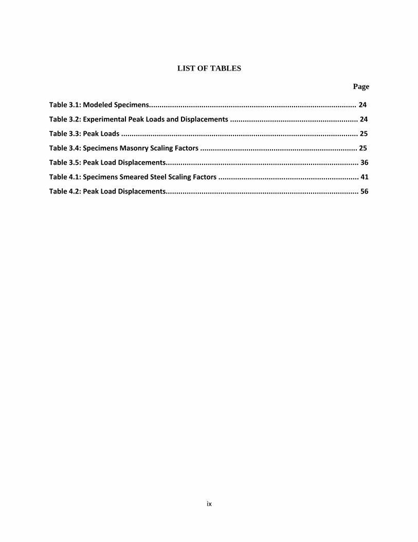
LIST OF TABLES
Page
Table 3.1: Modeled Specimens................................................................................................... 24
Table 3.2: Experimental Peak Loads and Displacements ............................................................. 24
Table 3.3: Peak Loads ................................................................................................................. 25
Table 3.4: Specimens Masonry Scaling Factors ........................................................................... 25
Table 3.5: Peak Load Displacements............................................................................................ 36
Table 4.1: Specimens Smeared Steel Scaling Factors ................................................................... 41
Table 4.2: Peak Load Displacements............................................................................................ 56

x
LIST OF FIGURES
Page
Figure 1.1: Basic Structural Configuration of Reinforced masonry walls (Klinger, 2010) ............... 2
Figure 1.2: Typical Reinforcement in Masonry Walls (Klinger, 2010) ............................................. 3
Figure 2.1: Experimental stress-stain curves for grouted/hollow concrete masonry (Chemma and
Klinger, 1986) ………………………………………………………………………………………………………………………….. 6
Figure 2.2: Experimental stress-stain curves for hollow concrete blocks (Barbosa and Hanai, 2009)
………………………………………………………………………………………………………………………………………………... 7
Figure 2.3: Experimental stress-stain curves for confined/unconfined concrete masonry compared
to modified Kent-Park (Priestley, 1986) ……………………………………………………………………………………. 7
Figure 2.4: Reinforced Masonry Wall Deformation mechanisms (Shing et al., 1990) …………………. 9
Figure 3.1: Scaling Relation of Stress-Strain in Compression between Masonry and Concrete ... 14
Figure 3.2: Scaling Relation of Stress-Strain in Tension between Masonry and Concrete …………. 14
Figure 3.3: Bi-Linear Stress-Strain Representation of Reinforcement Steel ……………………………... 15
Figure 3.4: Stress-Strain of Masonry in Compression for a Coarse Mesh …………………………………. 15
Figure 3.5: Stress-Strain of Masonry in Tension for a Coarse Mesh …………………………………………. 15
Figure 3.6: Typical Cantilever Masonry Walls …………………………………………………………………………. 16
Figure 3.7: Masonry Wall Cracked Section ……………………………………………………………………………… 16
Figure 3.8: Beam Cracked Section ………………………………………………………………………………………….. 17
Figure 3.9: Deflection of Reinforced Concrete Beams (Nilson et al., 2003) …………………………...... 19
Figure 3.10: Masonry Wall FE Model ………………………………………………….……………………....…………. 21
Figure 3.11: Meshing of the FE Model ……………………………………………………………………………………. 22
Figure 3.12: Loading of the FE Model ……………………………………………………………………………………… 22
Figure 3.13: Wall 1 (1/4 Spacing Mesh) Results ………………………………………………………………………. 28
Figure 3.14: Wall 1 (1/2 Spacing Mesh) Results ………………………………………………………………………. 29
Figure 3.15: Wall 1 (Spacing Mesh) Results ……………………………………………………………….……………. 30
Figure 3.16: Wall 8 (1/4 Spacing Mesh) Results ………………………………………………………………………. 32
Figure 3.17: Wall 8 (1/2 Spacing Mesh) Results ………………………………………………………………………. 33
Figure 3.18: Wall 8 (Spacing Mesh) Results ………………………….…………………………………………………. 34
Figure 4.1: Stress-Strain of Smeared Steel ………………………………………………………………………………. 37

xi
Figure 4.2: Equivalent Steel Springs …………………………………………………………………………………..…… 38
Figure 4.3: Reinforcement Steel Smearing on Structure Level …………………………………….………….. 39
Figure 4.4: Wall 1 (1/4 Spacing Mesh) Results ……………………………………………….………………….. 43-44
Figure 4.5: Wall 1 (1/2 Spacing Mesh) Results ……………………….……………………….…………………. 45-46
Figure 4.6: Wall 1 (Spacing Mesh) Results ……………………………..……………………….…………………. 47-48
Figure 4.7: Wall 8 (1/4 Spacing Mesh) Results ……………………………………………….………………….. 50-51
Figure 4.8: Wall 8 (1/2 Spacing Mesh) Results ……………………………………………….………………….. 52-53
Figure 4.9: Wall 8 (Spacing Mesh) Results ……………………………..……………………….…………………. 54-55
Figure A1.1: Wall 1 (1/4 Spacing Mesh) Results …………………………………………………………..…………. 64
Figure A1.2: Wall 1 (1/2 Spacing Mesh) Results …………………………………………………………..…………. 65
Figure A1.3: Wall 1 (Spacing Mesh) Results …………………………………….…………………………..…………. 66
Figure A1.4: Wall 2 (1/4 Spacing Mesh) Results …………………………………………………………..…………. 67
Figure A1.5: Wall 2 (1/2 Spacing Mesh) Results …………………………………………………………..…………. 68
Figure A1.6: Wall 2 (Spacing Mesh) Results …………………………………….…………………………..…………. 69
Figure A1.7: Wall 3 (1/4 Spacing Mesh) Results …………………………………………………………..…………. 70
Figure A1.8: Wall 3 (1/2 Spacing Mesh) Results …………………………………………………………..…………. 71
Figure A1.9: Wall 3 (Spacing Mesh) Results …………………………………….…………………………..…………. 72
Figure A1.10: Wall 4 (1/4 Spacing Mesh) Results …………………………….…………………………..…………. 73
Figure A1.11: Wall 4 (1/2 Spacing Mesh) Results ………………………………………………………..…………. 74
Figure A1.12: Wall 4 (Spacing Mesh) Results ………………………………….…………………………..…………. 75
Figure A1.13: Wall 5 (1/4 Spacing Mesh) Results ………………………………………………………..…………. 76
Figure A1.14: Wall 5 (1/2 Spacing Mesh) Results ………………………………………………………..…………. 77
Figure A1.15: Wall 5 (Spacing Mesh) Results ………………………………….…………………………..…………. 78
Figure A1.16: Wall 6 (1/4 Spacing Mesh) Results ………………………………………………………..…………. 79
Figure A1.17: Wall 6 (1/2 Spacing Mesh) Results ………………………………………………………..…………. 80
Figure A1.18: Wall 6 (Spacing Mesh) Results ………………………………….…………………………..…………. 81
Figure A1.19: Wall 7 (1/4 Spacing Mesh) Results ………………………………………………………..…………. 82
Figure A1.20: Wall 7 (1/2 Spacing Mesh) Results ………………………………………………………..…………. 83
Figure A1.21: Wall 7 (Spacing Mesh) Results ………………………………….…………………………..…………. 84
Figure A1.22: Wall 8 (1/4 Spacing Mesh) Results ………………………………………………………..…………. 85
Figure A1.23: Wall 8 (1/2 Spacing Mesh) Results ………………………………………………………..…………. 86

xii
Figure A1.24: Wall 8 (Spacing Mesh) Results ………………………………….…………………………..…………. 87
Figure A2.1: Wall 1 (1/4 Spacing Mesh) Results …………………………………………….………………….. 88-89
Figure A2.2: Wall 1 (1/2 Spacing Mesh) Results …………………………………………….………………….. 90-91
Figure A2.3: Wall 1 (Spacing Mesh) Results …………………………….…………………….………………….. 92-93
Figure A2.4: Wall 2 (1/4 Spacing Mesh) Results …………………………………………….………………….. 94-95
Figure A2.5: Wall 2 (1/2 Spacing Mesh) Results …………………………………………….………………….. 96-97
Figure A2.6: Wall 2 (Spacing Mesh) Results …………………………….…………………….………………….. 98-99
Figure A2.7: Wall 3 (1/4 Spacing Mesh) Results …………………………………………….…………..….. 100-101
Figure A2.8: Wall 3 (1/2 Spacing Mesh) Results …………………………………………….……………….. 102-103
Figure A2.9: Wall 3 (Spacing Mesh) Results …………………………….…………..…….………………….. 104-105
Figure A2.10: Wall 4 (1/4 Spacing Mesh) Results ……………………………………….………………….. 106-107
Figure A2.11: Wall 4 (1/2 Spacing Mesh) Results ……………………………………….………………….. 108-109
Figure A2.12: Wall 4 (Spacing Mesh) Results ………………..……….………………….………………….. 110-111
Figure A2.13: Wall 5 (1/4 Spacing Mesh) Results ……………………………………….………………….. 112-113
Figure A2.14: Wall 5 (1/2 Spacing Mesh) Results ……………………………………….………………….. 114-115
Figure A2.15: Wall 5 (Spacing Mesh) Results ………………..……….………………….………………….. 116-117
Figure A2.16: Wall 6 (1/4 Spacing Mesh) Results ……………………………………….………………….. 118-119
Figure A2.17: Wall 6 (1/2 Spacing Mesh) Results ……………………………………….………………….. 120-121
Figure A2.18: Wall 6 (Spacing Mesh) Results ………………..…….…………………….………………….. 122-123
Figure A2.19: Wall 7 (1/4 Spacing Mesh) Results ……………………………………….………………….. 124-125
Figure A2.20: Wall 7 (1/2 Spacing Mesh) Results ……………………………………….………………….. 126-127
Figure A2.21: Wall 7 (Spacing Mesh) Results ……………..……….…………………….………………….. 128-129
Figure A2.22: Wall 8 (1/4 Spacing Mesh) Results ……………………………………….………………….. 130-131
Figure A2.23: Wall 8 (1/2 Spacing Mesh) Results ……………………………………….………………….. 132-133
Figure A2.24: Wall 8 (Spacing Mesh) Results ……………..……….…………………….………………….. 134-135

xiii
List of Symbols
crA Cracked Area of Masonry Section ( 2in )
sA Total Steel Area ( 2in )
sbA Area of Single Steel Bar ( 2in )
sxA Area of Reinforced Steel in X-Direction ( 2in )
syA Area of Reinforced Steel in Y-Direction ( 2in )
b Masonry Wall Width ( in )
'b Smeared Steel Element Width ( in )
][C Damping Matrix
d Depth of Steel Reinforcement Measured from Top Compression Fibers ( in )
eqE Equivalent Masonry Modulus of Elasticity ( psi )
mE Masonry Modulus of Elasticity ( psi )
sxE Equivalent Smeared Steel Modulus of Elasticity in X-Direction ( psi )
syE Equivalent Smeared Steel Modulus of Elasticity in Y-Direction ( psi )
sE Steel Modulus of Elasticity ( psi )
EI Flexural Stiffness
e Reinforcement Steel Bars Edge Distance ( in )
mf Compressive Stress in Masonry Top Fibers ( psi )
'mf Compressive Stress of Masonry Prism ( psi )
sf Tensile Stress of Steel Reinforcement ( psi )
tf Maximum Tensile Stress of Masonry ( psi )
uf Ultimate Steel Stress ( psi )
xiv
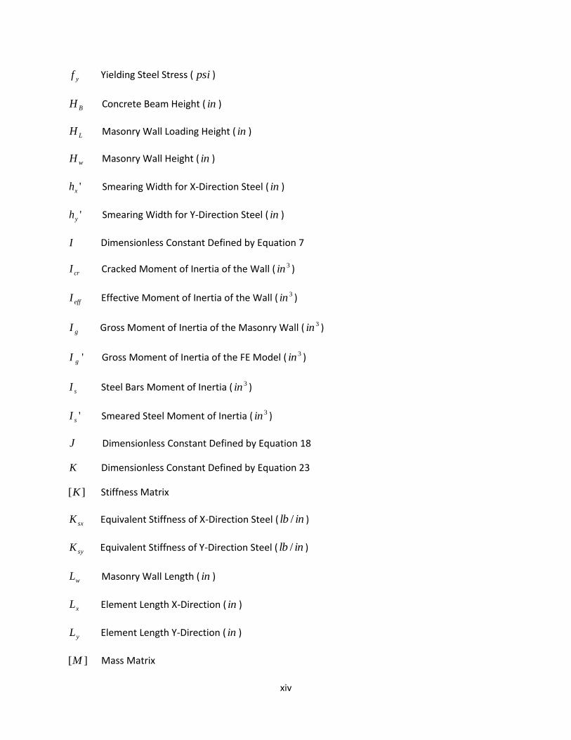
yf Yielding Steel Stress ( psi )
BH Concrete Beam Height ( in )
LH Masonry Wall Loading Height ( in )
wH Masonry Wall Height ( in )
'xh Smearing Width for X-Direction Steel ( in )
'yh Smearing Width for Y-Direction Steel ( in )
I Dimensionless Constant Defined by Equation 7
crI Cracked Moment of Inertia of the Wall ( 3in )
effI Effective Moment of Inertia of the Wall ( 3in )
gI Gross Moment of Inertia of the Masonry Wall ( 3in )
'gI Gross Moment of Inertia of the FE Model ( 3in )
sI Steel Bars Moment of Inertia ( 3in )
'sI Smeared Steel Moment of Inertia ( 3in )
J Dimensionless Constant Defined by Equation 18
K Dimensionless Constant Defined by Equation 23
][K Stiffness Matrix
sxK Equivalent Stiffness of X-Direction Steel ( inlb / )
syK Equivalent Stiffness of Y-Direction Steel ( inlb / )
wL Masonry Wall Length ( in )
xL Element Length X-Direction ( in )
yL Element Length Y-Direction ( in )
][M Mass Matrix

xv
aM Applied Moment ( inlb. )
crM Cracking Moment ( inlb. )
yM Yielding Moment ( inlb. )
N No. of Vertical Steel Bars
n Modeler Ratio
P Total Axial Load on the Wall, Including Own Weight ( lb )
sxP Axial Load in Equivalent X-Direction Spring ( lb )
syP Axial Load in Equivalent Y-Direction Spring ( lb )
S Vertical Steel Bars Spacing ( in )
mw Masonry Unit Weight ( pcf )
x Position of the Neutral Axis Measured From Compression Top Fibers ( in )
c Ratio of Mass Damping
m Coarse Meshing Masonry Scaling Factor
s Smeared Steel Scaling Factor
sx X-Direction Smeared Steel Scaling Factor
sy Y-Direction Smeared Steel Scaling Factor
Stiffness Modification Factor
c Ratio of Stiffness Damping
x X-Direction Displacement ( in )
y Y-Direction Displacement ( in )
m Compressive Stain in Masonry at the Top Fibers
s Tensile Stain of Steel
xvi
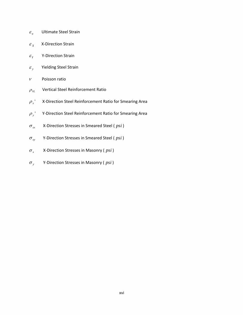
u Ultimate Steel Strain
X X-Direction Strain
Y Y-Direction Strain
y Yielding Steel Strain
Poisson ratio
VL Vertical Steel Reinforcement Ratio
'x X-Direction Steel Reinforcement Ratio for Smearing Area
'y Y-Direction Steel Reinforcement Ratio for Smearing Area
sx X-Direction Stresses in Smeared Steel ( psi )
sy Y-Direction Stresses in Smeared Steel ( psi )
x X-Direction Stresses in Masonry ( psi )
y Y-Direction Stresses in Masonry ( psi )

1
CHAPTER ONE
INTRODUCTION
1.1 Historical Background
Since ancient times, masonry has been a common construction material for many types of
structures, including buildings and bridges. This may be easily seen in the structures that remain
from antiquity, such as those of the Romans. Although their construction might seem elementary, a
good engineering sense was needed to design structures that have only compression internal
forces, such as arched structures, since masonry does not have significant tensile resistance.
Masonry is still widely used in the U.S. as the basis of many structural elements, such as
beams, columns, and walls. In order to enhance the tensile behavior and ductility of masonry
structures, steel reinforcement is used to resist tensile stresses.
1.2 Masonry Wall Construction
In order to understand the behavior of masonry walls, it is necessary to discuss the
elements that are used to construct the wall itself. Typically, masonry walls are composed of the
following: masonry units, mortar joints, grout, and steel reinforcement, as shown in Figure 1.1
(Klingner, 2010)
1.2.1 Masonry Units
Masonry units are considered to be the main item in the wall composition. They are used to
fill the space that is required to be filled architecturally and they provide the major contribution to
the required compressive strength for resisting the structural loads. There are many types of these
units. Examples include clay masonry units, which are formed from clay and sedimentary minerals
with a compressive strength that varies from 1200 to 30,000 psi, and concrete masonry units, which
are formed from zero-slump concrete with a compressive strength of 1500 to 3000 psi. (Klingner,
2010)

2
Figure 1.1 Basic Structural Configuration of Reinforced masonry walls (Klingner, 2010)
1.2.2 Mortar Joints
Mortar joints are used to hold masonry units together and also apart from each other due
to dimensional tolerances. Horizontal joints are called bed joints and vertical joints are called head
joints. There are three types of cementitious systems used as masonry mortar: Cement-Lime
mortar, Masonry-Cement mortar, and Mortar-Cement mortar (Klingner, 2010). Mortar types are
classified as: Type M which has high compressive and tensile bond strength, Type S which has
moderate compressive and tensile bond strength, Type N which has low compressive and tensile
bond strength, and Type O which has very low compressive and tensile bond strength. (Klingner,
2010)
1.2.3 Reinforcement
Reinforcement bars are used in masonry construction to resist tensile stress in the wall and
increase wall ductility and resistance against vertical and lateral loads due to wind and earthquakes.
Several kinds of reinforcement are commonly used: steel deformed bars, as shown in Figure 1.2(a),
joint reinforcement, deformed reinforcing wires, steel welded wire reinforcement, as shown in
Figure 1.2(b), and steel pre-stressing strands, as shown in Figure 1.2(c) (Klingner, 2010).

3
(a) (b) (c)
Figure 1.2 Typical Reinforcement in Masonry Walls (Klingner, 2010)
1.2.4 Grout
Grout is a cementitious fluid composed of Portland cement, sand, and pea gravel. It is used
as a fluid to fill spaces in masonry and to surround reinforcement bars in order to enhance bond
characteristics. (Klingner, 2010)
1.3 Masonry Research
As with any construction material, many studies have focused on the behavior of the
masonry itself, and also on that of masonry structures.
1.3.1 Experimental Research
Early studies on masonry focused on the general behavior of either the masonry as a
composite of several materials, or on each of its components separately. There are many
uncertainties about the behavior of the individual masonry constituents. Therefore, the overall
failure criteria for masonry structures are very complicated as their performance involves the
interaction of several different components.
Other studies have focused on the behavior of masonry structures, especially masonry
walls. These kinds of studies focused on the effect of wall dimensions and the use of different types
of masonry, mortar, and/or grout on the bending and shear behavior of the wall, as is discussed in
Chapter 2.

4
1.3.2 Modeling Research
In parallel with experimental studies, many models have been proposed to simulate the
behavior of masonry materials and/or structures. These models have been formulated from
different theoretical bases, including fracture energy, damage mechanics, and plasticity.
In general, there are two main approaches for the modeling of masonry structures: 1) to
model each component of masonry separately, which is called micro modeling, and 2) to model the
masonry structures using one equivalent material, which is called macro modeling.
1.4 Research Objectives
The main objective of this research is to simplify the nonlinear finite element modeling of
masonry walls. The modeling simplification was based on two ideas, which are:
1) Developing a consistent approach for the masonry material in order to use it in macro-
modeling, and
2) Using smeared reinforcing steel instead of discrete bars.
Also, coarse meshing and a relatively large time steps are considered in order to decrease
the time and effort of analysis. The overall intent is to provide an accurate, but simplified,
representation of reinforced masonry shear walls that can be used as part of a larger model of an
entire structure.
5
CHAPTER TWO
LITERATURE REVIEW
2.1 Introduction
Although research on masonry started early in the twentieth century, there is great
variation in the results of each research study, especially regarding the masonry material behavior
itself. The reason is that masonry structures are constructed from different materials and the fact
that the construction procedure itself leads to high variance due to human involvement. The main
objective of this chapter is to review the previous work done in the following fields: 1) Masonry
material behavior, 2) Masonry wall general behavior, and 3) modeling of masonry structures.
2.2 Masonry failure behavior
Failure behavior of masonry is very complicated and different from most other composite
materials. Unlike other materials, failure of masonry can be caused by mortar joint failure, which is
more like micro scale failure, or crushing of masonry units along with mortar, which is more like
macro scale failure. This unique behavior implies that the general performance of masonry is
strongly affected by the orientation of masonry and mortar, in addition to the behavior of the
components. This leads to anisotropic behavior for masonry.
Many studies have focused on the in-plane behavior of concrete masonry under biaxial
tension-compression, especially grouted masonry. The main conclusion was that grouted concrete
masonry behaves as an anisotropic material, the properties of which depend on bed joint
orientation (Drysdale and Khattab, 1995). However, this anisotropic behavior does not have a
significant effect on the macro-scale behavior (Karapitta et al., 2011), so it can be reasonably
represented as being orthotropic, similar to the orthotropic behavior of concrete.
2.2.1 Compressive behavior of masonry
The compressive behavior of masonry is very complicated because of the interaction of
different materials, each having individual failure mechanisms. In order to monitor this behavior,
masonry prisms with the same construction are often used. The major contribution to compressive
resistance comes from the blocks, but there are other factors that also affect the compressive
resistance, such as: block geometry, height to thickness ratio of the block, mortar bedding, and
6
thickness of the mortar joint (Ramamurthy et al., 2000). Also, load eccentricity has a great effect on
the compressive behavior, which increases with a decrease of the block solid percentage (Drysdale
and Hamid, 1983).
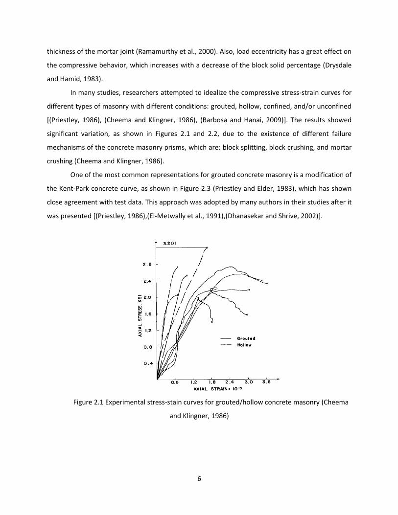
In many studies, researchers attempted to idealize the compressive stress-strain curves for
different types of masonry with different conditions: grouted, hollow, confined, and/or unconfined
[(Priestley, 1986), (Cheema and Klingner, 1986), (Barbosa and Hanai, 2009)]. The results showed
significant variation, as shown in Figures 2.1 and 2.2, due to the existence of different failure
mechanisms of the concrete masonry prisms, which are: block splitting, block crushing, and mortar
crushing (Cheema and Klingner, 1986).
One of the most common representations for grouted concrete masonry is a modification of
the Kent-Park concrete curve, as shown in Figure 2.3 (Priestley and Elder, 1983), which has shown
close agreement with test data. This approach was adopted by many authors in their studies after it
was presented [(Priestley, 1986),(El-Metwally et al., 1991),(Dhanasekar and Shrive, 2002)].
Figure 2.1 Experimental stress-stain curves for grouted/hollow concrete masonry (Cheema
and Klingner, 1986)

7
Figure 2.2 Experimental stress-stain curves for hollow concrete blocks (Barbosa and Hanai,
2009)
Figure 2.3 Experimental stress-stain curves for confined/unconfined concrete masonry
compared to modified Kent-Park (Priestley, 1986)

8
2.2.2 Tensile Behavior of Masonry
Masonry has very low tensile strength, such that it can be ignored. Tensile behavior is
mainly governed by mortar joint splitting. As the setup of a test is nearly impossible, no significant
research has been done to monitor the tensile stress-strain behavior of masonry prisms using a
direct tensile test. Most authors use the tensile stress-strain curve proposed for concrete (Haach et
al., 2011), having both ascending and softening parts, with much lower tensile resistance as
recommended by codes (Horton and Tadros, 1990) or obtained from indirect tensile tests (Drysdale
et al., 1979).
2.3 Masonry Wall Lateral Behavior
The behavior of masonry walls can be described from the perspective of micro or macro
behavior. The macro approach is most convenient for studying the overall behavior of the wall
because it considers the wall as being constructed of one homogenous material. On the other hand,
with the micro approach, the behavior of the wall is represented through localized
cracking/crushing of the masonry units and failure at mortar joints. This approach is suitable for
small structures, but it becomes very complicated with large ones.
2.3.1 In-Plane Behavior
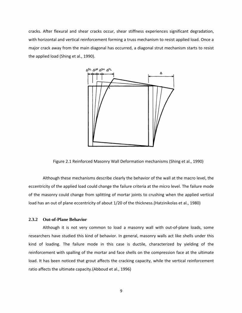
The total lateral deformation of a masonry wall is the summation of four distinct
mechanisms: base sliding, overall shear distortion, apparent flexural deformation which includes
the base uplift due to bond slip and elongations of vertical steel, and flexural deformation
calculated from section curvature, as shown in Figure 2.1. (Shing et al., 1990)
It is very difficult to measure the bond slip of the wall, so it is not usually possible to isolate
the base uplift from the total flexural displacement. In reality, because it is very difficult to calculate
the flexural deformation, it is usually obtained experimentally by subtracting shear base sliding and
shear distortion from total displacement. For some cases, base sliding is insignificant, so it can be
ignored for theoretical calculations of flexural displacement. However, in the case of low rise walls,
it usually has a significant effect on overall displacement. (Shing et al., 1990)
For shear deformation calculations, the wall panel can be considered as a linear elastic
section with the effect of reinforcement on shear stiffness being negligible until the occurrence of
9
cracks. After flexural and shear cracks occur, shear stiffness experiences significant degradation,
with horizontal and vertical reinforcement forming a truss mechanism to resist applied load. Once a
major crack away from the main diagonal has occurred, a diagonal strut mechanism starts to resist
the applied load (Shing et al., 1990).
Figure 2.1 Reinforced Masonry Wall Deformation mechanisms (Shing et al., 1990)
Although these mechanisms describe clearly the behavior of the wall at the macro level, the
eccentricity of the applied load could change the failure criteria at the micro level. The failure mode
of the masonry could change from splitting of mortar joints to crushing when the applied vertical
load has an out of plane eccentricity of about 1/20 of the thickness.(Hatzinikolas et al., 1980)
2.3.2 Out-of-Plane Behavior
Although it is not very common to load a masonry wall with out-of-plane loads, some
researchers have studied this kind of behavior. In general, masonry walls act like shells under this
kind of loading. The failure mode in this case is ductile, characterized by yielding of the
reinforcement with spalling of the mortar and face shells on the compression face at the ultimate
load. It has been noticed that grout affects the cracking capacity, while the vertical reinforcement
ratio affects the ultimate capacity.(Abboud et al., 1996)

10
2.4 Modeling of Masonry walls
Many studies have focused on the different methods for modeling masonry structures but,
as mentioned earlier, these studies can be categorized under two main approaches: Micro-
Modeling and Macro-Modeling. In micro-modeling, it is considered as a discrete assembly of units
with different, while in properties macro-modeling, masonry is considered to be a homogenous
material with equivalent properties (Haach et al., 2011).
2.4.1 Micro-Modeling
Micro-modeling is the most common technique used for small structures and/or for
studying the effect of each component’s local failure mechanisms on the general behavior. It can be
simply described as discretizing each component of the model, and using different elements and
constitutive models for each one.
The same concept is used in masonry modeling, but it is not applicable to large structures
due to the relatively small dimensions of the masonry and mortar compared with those of the
structure, which requires a very fine mesh. The main elements used in this kind of modeling are
masonry elements, mortar joint elements, and masonry-mortar interface elements.
However, most researchers do not apply such detail for their micro-modeling because it
requires a very fine mesh due to the very small thickness of the mortar joints. The most common
approach for the discretization is to use two different types of elements, one for the masonry units
and mortar joints, as a homogenous material, and the other as zero thickness interface elements for
potential cracks [(Loureco and Rots, 1997),(Gambarotta and Lagomarsino, 1997),(Chaimoon and
Attard, 2007), (Da Porto et al., 2010), (Haach et al., 2011)]. With this approach, the effort required
for computation is reduced because of the ability to use a coarser mesh.
Typically, the micro-modeling technique allows the use of different mechanical assumptions
for materials, such as damage models (Gambarotta and Lagomarsino, 1997), cap models (Loureco
and Rots, 1997), and/or fracture models (Chaimoon and Attard, 2007), to study the behavior of
masonry , with monotonic (Haach et al., 2011) or cyclic loading (Da Porto et al., 2010).
2.4.2 Macro-Modeling
The macro-modeling approach is the most common technique used for large structures
and/or for studying the effect of global parameters, such as compressive strength, reinforcement

11
ratio, and structure dimensions, on the general structural behavior. It can be simply described as
modeling the overall structure with one homogeneous material, which has properties that are
equivalent to the sum of its components.
This method is convenient for both analytical and numerical modeling because it does not
require the level of detailed discretization used for micro-modeling, which is based on individual
material components.
2.4.2.1 Macro-Modeling for Concrete.
Macro-modeling is very common for concrete structures because it is very difficult to model
the aggregates and the cementitious components separately. Many researchers have proposed
constitutive relations and failure criteria for concrete [e.g. Modified compression field theory
(Vecchio and Collins, 1986)] and have used these to model and predict the behavior of various
concrete structures [e.g., (Vecchio, 1990), (Selby and Vecchio, 1997), (Vecchio and Selby, 1991)].
In addition, reinforcement has been treated on the macro-scale as individual embedded
elements within concrete elements (Yamaguchi and Ohta, 1993) or through smearing the
reinforcement properties within concrete elements (Kazaz et al., 2006).
Finally, for most studies, the smeared crack model has been used for equivalent cracking
behavior (Balakrishnan and Murray, 1988), which can be developed with fracture energy (Feenstra
and De Borst, 1995) in order to achieve mesh size independence.
2.4.2.2 Macro-Modeling for Masonry.
In parallel with the aforementioned concrete studies, many researchers have attempted to
model masonry structures at the macro level. However, unlike concrete, macro-modeling of
masonry structures is very complicated because of their anisotropic nature and the local failure
mechanisms that govern their global failure.
As previously mentioned, both analytical and numerical models can be developed with
macro-modeling. Analytical modeling is usually used to predict the general behavior of simple
structures with simple types of loads. For example, Horton and Tadros (1990) used various
approaches and methods for estimating effective stiffness, including the ACI formula for concrete,
in order to calculate the deflection of masonry flexural members. El-Metwally et al. (1991) used a
model of an equivalent plane strain beam column to model a strip of masonry wall subjected to

12
eccentric uniform load. The predicted capacity was found to be very sensitive to end eccentricity,
especially in short walls.
For more sophisticated structures and loading, numerical analysis based on the finite
element method is used. For example, Afshari and Kaldjian (1989) used finite element analysis to
predict the failure envelope for masonry walls. They used 8-node three dimensional elements for
the wall, and they assumed linear analysis for brittle cementitious materials such as blocks, grout,
and mortar. The proposed failure envelope, which is based on basic strength and geometric
characteristic values of mortar joints and masonry units, showed good agreement with
experimental results. Loureco et al. (1998) developed a continuum model for masonry. The model
was based on orthotropic elasto-plasticity, such that uniaxial tension and compression behavior
could be described. Two main failure mechanisms were assumed: localized and distributed fracture.
Mojsilovic and Marti (1997) presented a sandwich model to predict the strength of masonry wall
elements subjected to combined in-plane forces and moments. Legeron et al. (2005) used a finite
element analysis based on multilayer elements with damage mechanics to model monotonic and
cyclically loaded reinforced concrete structures. Sutcliffe et al. (2001) used the lower bound theory
of classical plasticity to estimate the lower bound load of unreinforced masonry shear walls. Asteris
and Tzamtzis (2003) developed a yielding surface, as a failure criterion, for macro-modeling of
masonry walls. El-Dakhakhni et al (2006) used a multilaminate model for concrete masonry walls.
The masonry was modeled as a homogenous medium, overlaid with two sets of planes of
weakness, representing head and bed joints, and two sets of reinforcement. The effects of
weakness planes and reinforcement were smeared within the masonry elements. Stavridis and
Shing (2010) modeled masonry-infilled RC Frames considering a combination of the smeared and
discrete crack approaches in order to capture the different failure modes. Karapitta et al (2011)
used explicit dynamic analysis to model the cyclic behavior of unreinforced masonry. A micro-model
was used based on a coaxial-total-based rotation smeared crack model. A material constitutive law
based on fracture energy was also proposed.

13
CHAPTER THREE
DISCRETIZED STEEL MODEL
3.1 Introduction
In this chapter, the modeling of a masonry wall through the application of a macro approach
with coarse meshing and smeared cracking for the masonry material and discretized axial elements
for steel reinforcement is described. Although this model requires a high level of detail due to the
representation of steel as a set of discretized axial elements, it is required to validate the modeling
technique. The idea presented in this chapter is to scale the masonry constitutive relations so that
they represent the stiffness degradation of the masonry wall due to crack propagation.
3.2 Material Assumptions
Within the modeling process, the constitutive relations of masonry at the macro scale and
the model for the reinforcing steel have significant effects on the final results. The material
assumptions used in the modeling are discussed in this section.
3.2.1 Masonry
As discussed in Chapter 2, the macro behavior of masonry is similar to the behavior of
concrete in tension and compression. The initial tangent modulus of elasticity of masonry can be
estimated as in Equation 1 (Holm, 1987), where a unit weight of 125 pcf is used, which is in a format
similar to that for the initial tangent modulus of elasticity of concrete.
'**225.1
mmm fwE [1]
In this research, the overall stress-strain curve of masonry is assumed to be a horizontal
(strain) scaling of the stress-strain curve of concrete, with the scaling factor equal to the ratio of
their initial tangent moduli of elasticity for the same stress, as shown in Figure 3.1.

14
Figure 3.1 Scaling Relation of Stress-Strain in Compression between Masonry and Concrete
Also, tensile behavior is assumed to be the same as that of concrete, as shown in Figure3.2,
with the same scaling as that used for compression. The ultimate cracking stress is reported to vary
from 'mf to '5 mf (Horton and Tadros, 1990), based on masonry type, mortar, and grouting. The
limit used in Equation 2 was recommended by the Uniform Building Code (Horton and Tadros,
1990).
'5.2 mt ff [2]
Figure 3.2 Scaling Relation of Stress-Strain in Tension between Masonry and Concrete
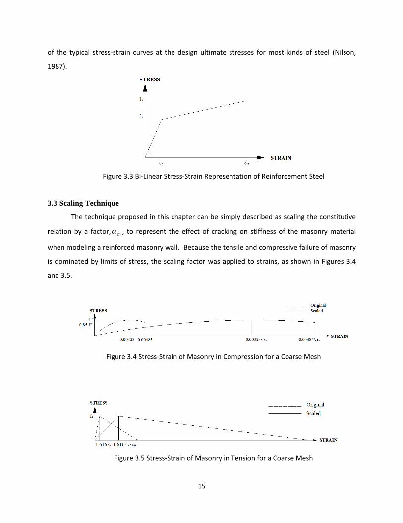
3.2.2 Reinforcement Steel
The constitutive relation used for steel is a bilinear representation with strain hardening, as
shown in Figure 3.3. The ultimate strain is assumed to be 0.021, based on the tangent intersection
15
of the typical stress-strain curves at the design ultimate stresses for most kinds of steel (Nilson,
1987).
Figure 3.3 Bi-Linear Stress-Strain Representation of Reinforcement Steel
3.3 Scaling Technique
The technique proposed in this chapter can be simply described as scaling the constitutive
relation by a factor, m , to represent the effect of cracking on stiffness of the masonry material
when modeling a reinforced masonry wall. Because the tensile and compressive failure of masonry
is dominated by limits of stress, the scaling factor was applied to strains, as shown in Figures 3.4
and 3.5.
Figure 3.4 Stress-Strain of Masonry in Compression for a Coarse Mesh
Figure 3.5 Stress-Strain of Masonry in Tension for a Coarse Mesh

16
3.3.1 Scaling due to Material Behavior
The scaling factor m is the reduction required to be applied to the initial modulus of
elasticity acting with the gross overall moment of inertia of the wall, such that the flexural stiffness
is equivalent to the initial modulus of elasticity acting on the cracked moment of inertia of the wall.
This approach is necessary to properly consider the reduction in stiffness due to initial cracking of
the wall, which is not considered in a finite element model. The reduction factor is defined on the
basis of a cracked wall cross section.
Typically, masonry wall test specimens can be loaded through a concrete loading beam, as
shown in Figure 3.6(a), or the load can be applied directly to the wall, as shown in Figure 3.6(b). For
typical cantilever masonry walls, the cracked cross section of the base at working load is shown in
Figure 3.7.
a) Masonry Wall with Concrete Beam b) Masonry Wall without Concrete Beam
Figure 3.6 Typical Cantilever Masonry Walls
Figure 3.7 Masonry Wall Cracked Section

17
In the case of applied moment only, without axial load, the position of the neutral axis can
be obtained by taking the moment of areas about the neutral axis.
N
i
sbsb xnNAbxSienAbx
1
2
)())1((2
[3]
where
m
s
E
En
[4]
The equation can be simplified as
02
2 InAxnNAxb
sbsb
[5]
where
)(5.0)( 2NNSNseI [6]
From the solution of the quadratic equation,
b
IbnAnNAnNAx
sbsbsb 2)( 2
[7]
However, in a general loading condition, the wall is subjected also to axial load. For the
simple case of a beam subjected to both bending moment and axial load at the working stage, as
shown in Figure 3.8, the position of the neutral axis can be obtained from internal force equilibrium.
Figure 3.8 Beam Cracked Section
PfAbxf ssm '5.0
[8]
By replacing stresses with strains,
PEAbxE sssmm 5.0
[9]

18
From the plane section assumption,
x
xd
m
s
[10]
By substituting into the internal force equation,
m
smE
P
x
xdnAbx
)5.0(
[11]
The final formula can be represented as
xf
PxdnA
bx
m
s )(2
2
[12]
The previous equation is analogous to equation 5, which can be modified as
xf
PInAxnNAx
b
m
sbsb 2
2
[13]
The position of the neutral axis is
b
IbnAf
PnNA
f
PnNA
x
sb
m
sb
m
sb 2)()( 2
[14]
In the previous equation, the maximum compressive stress mf in masonry is required to find
the position of the neutral axis. This stress value can be defined as
crcr
a
mA
Px
I
Mf
[15]
The cracked moment of inertia is
JnAbx
I sbcr 3
3
[16]
where
SNNN
SNNxseNxsexSieJN
i
)326
())(()())1((32
22
1
2
[17]
and the cracked area is
sbcr nNAbxA
[18]
Also, the applied moment aM is required. In the case of collapse analysis, yielding moment
yM should be used instead of applied moment, which can be calculated as

19
))1((
)(
xSNe
IA
P
n
f
M
cr
cr
y
y
[19]
The previous set of equations requires an iterative process because the position of the
neutral axis governs the moment of inertia, area, masonry compressive stress, and yielding moment
calculations.
As masonry behaves like concrete, the stiffness of the wall passes through two stages: first,
the wall behaves as an uncracked section until it reaches the cracking moment, at which point it
behaves as a cracked section, as shown in Figure 3.9
Figure 3.9 Deflection of Reinforced Concrete Beams (Nilson et al., 2003)
In order to represent this change in moment of inertia, an effective moment of inertia can
be used. The ACI equation for effective moment of inertia in concrete sections is also applicable for
masonry structures (Horton and Tadros, 1990).
g
a
cr
cr
a
cr
geff IM
MI
M
MII ))(1()( 33
[20]
The gross moment of inertia can be calculated as
KSnASNeb
I sbg
23
12
))1(2(
[21]
20
where
12
))2
1((
32 NNN
iK
[22]
The cracking moment is
))1(2(
)(2
SNe
IA
Pf
M
g
g
t
cr
[23]
where the gross area of the section would be
sbg nNASNebA ))1(2(
[24]
The final step is to find an equivalent modulus of elasticity to combine with the finite
element gross moment of inertia 'gI , leading to the same flexural stiffness:
'geqeffm IEIE
[25]
where
KSA
E
ESNebI sb
eq
s
g
23
12
))1(2('
[26]
By substituting from Equation 26 into Equation 25,
12/))1(2( 3
2
SNeb
KSAEIEE
sbseffm
eq
[27]
Finally, the scaling factor due to material behavior can be calculated as
12/))1(2( 3
2
SNeb
KSnAI
E
E sbeff
m
eq
m
[28]
3.4 Finite Element Model Description
In this study, the finite element program ADINA is used for modeling. In this section, the
details of the finite element model are described.
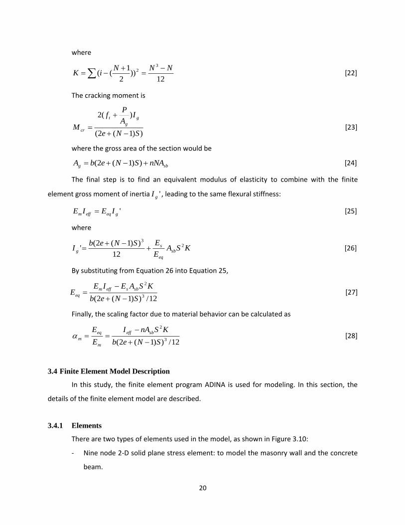
3.4.1 Elements
There are two types of elements used in the model, as shown in Figure 3.10:
- Nine node 2-D solid plane stress element: to model the masonry wall and the concrete
beam.

21
- 1-D axial truss element: to model the discretized steel reinforcement.
a) Masonry Walls with Concrete Beam b) Masonry Walls without Concrete Beam
Figure 3.10 Masonry Wall FE Model.
3.4.2 Materials
Three types of material models were used:
- Concrete material: to model the masonry wall. The concrete model in ADINA allows the
use of fracture energy to achieve mesh size independence.
- Elasto-plastic material: to model the reinforcement steel.
- Linear elastic material: to model the concrete loading beam, or the upper part of the
masonry wall above the applied load. The main purpose of these elements is to prevent
numerical local failure at the loading point.
3.4.3 Meshing
Different mesh sizes were considered for the models. To be consistent, mesh sizes of 1/4,
1/2, and 1 times the maximum reinforcement spacing were used, as shown in Figure 3.11.

22
a) 1/4 Spacing Mesh Size a) 1/2 Spacing Mesh Size a) Spacing Mesh Size
Figure 3.11 Meshing of the FE Model.
3.4.4 Loading
Besides a constant vertical load, a displacement type of loading was applied to the top of
the wall, as shown in Figure 3.12, with a step increment of 0.001 inch.
Figure 3.12 Loading of the FE Model.

23
3.4.5 Boundary Conditions
Vertical and horizontal displacements were constrained at the wall base to represent a full
fixity condition. Although wall sliding is a possible failure mode, which requires a different type of
boundary condition, this aspect of behavior was beyond the scope of this analysis, as it requires
further experimental study.
3.4.6 Model Kinematics
Nonlinear analysis with a large displacement formulation was considered, and the lateral
loading was applied through prescribed displacement for the purpose of expediting convergence.
3.4.7 Fictitious Dynamics
During an analysis, when the first element experiences cracking, its stiffness matrix is no
longer positive definite, which often leads to nonconvergence in the solution. In order to continue
with the analysis, the low speed dynamics (LSD) feature in ADINA was used. In that case, a fictitious
damping matrix is added to the model, as defined in Equation 29.
KMC cc
[29]
Because the analysis is still static and no mass was applied to the model, the fictitious
damping matrix only affects the stiffness matrix. The value of the coefficient c is recommended to
be defined as in Equation 30, and its default value is 0.0001 (ADINA, 2010). As long as the fictitious
dynamic force is less than 1% of the applied force, the static analysis is deemed to be unaffected by
the addition of the artificial damping.
510c
of Time Step Size
[30]
For consistency in the results, the default value of 0.0001 was used for all specimen models
with their different mesh sizes.
3.5 Modeled Specimens
Eight Specimens were modeled to investigate the validity of the proposed approach. The
first two specimens were a part of an experimental program that is concurrently taking place
(Sherman, 2011). The other six specimens were part of a previous experimental program (Eikanas,
2003). All specimens are described in Table 3.1, with reference to Figure 3.6.

24
Table 3.1 Modeled Specimens
Wall
Specimen .)(in
H w
.)(in
H L .)(in
Lw
wL LH /
Vert.
Reinf.
Horiz.
Reinf.
VL 'mf **
(Psi)
Axial
Load***
(Kips)
1* 72 80 40 2.00 "8@6#5 "8@4#9 0.0072 2775 48
2* 72 80 40 2.00 "8@4#5 "8@4#9 0.0032 2775 95
3 72 52 55.625 0.93 "16@5#4 "16@4#5 0.0031 1630 11.4
4 104 84 55.625 1.50 "16@5#4 "16@4#7 0.0031 1630 11.4
5 72 52 55.625 0.93 "8@5#7 "16@4#5 0.0055 1630 11.4
6 104 84 55.625 1.50 "8@5#7 "16@4#7 0.0055 1630 11.4
7 104 84 39.625 2.10 "8@5#5 "16@4#7 0.0057 1630 8.13
8 72 52 71.625 0.72 "16@5#5 "16@4#5 0.0030 1630 14.7
* Walls with concrete loading beam of 12 in width, 16 in height, and 44 in length.
** Average Prism Strength.
***Does not include self-weight of the wall.
All walls have thickness of 7.6 in
Grade 60 steel was used for reinforcement in all specimens, resulting in yield and ultimate
stress values in the finite element analyses of 60 and 75 Ksi, respectively.
Peak loads and their associated displacements (PLD) from experimental data are presented
in Table 3.2
Table 3.2 Experimental Peak Loads and Displacements
Specimen 1 2 3 4 5 6 7 8
Ultimate Load (Kips) 41.37 37.21 48.74 30.59 63.33 42.35 27.06 71.25
PLD (in) 1.1 0.55 0.7 0.59 0.57 0.95 0.58 0.27
For these specimens, nominal peak load was calculated using LRFD and presented in Table
3.3. By comparing the calculated and experimental peak loads, it was observed that the calculated
peak load varies from the experimental data by 0.3-24.7%. This can be explained in terms of the
variation of material properties.

25
Table 3.3 Peak Loads
Specimen 1 2 3 4 5 6 7 8
Peak
Load
(Kips)
Experimental 41.37 37.21 48.74 30.59 63.33 42.35 27.06 71.25
Calculated
(var. %)
37.04
(10.5)
31.65
(15.9)
42.61
(12.6)
29.5
(3.6)
63.53
(0.3)
39.33
(7.1)
20.38
(24.7)
68.78
(3.5)
All experimental specimens were cyclically loaded until failure. However, the FE analyses
were monotonic. In order to compare numerical and experimental results, the load-displacement
curves obtained from the FE model for each specimen were compared with the envelope defined
by experimental cycle peaks.
For each specimen, the suggested methodology was followed to consider the reduction in
stiffness from initial cracking. The Scaling factor m for each specimen, based on yield moment as
applied moment, is presented in Table 3.4.
Table 3.4 Specimen Masonry Scaling Factors
Specimen 1 2 3 4 5 6 7 8
m 0.204159 0.413914 0.157824 0.157824 0.169664 0.169556 0.168239 0.164426
The calculated scaling factors are similar to the moment of inertia reduction factors used to
estimate the actual cracked deflection of concrete members, which vary from 0.35 to 0.7 for
compression and flexural members in ACI 318-08 (2008). As expected, masonry values are lower
than concrete values because of lower masonry tensile strength, due to the interaction between
masonry units and mortar, and modulus of elasticity.
3.6 Results
Selected results for representative specimens are presented in the figures below. For each
case, the following items are shown:
- Deflected shape and crack pattern;
- Masonry principal stresses;
- Axial strain in steel; and

26
- Comparison between FE and experimental results.
Note that the “comparison between FE and experimental results” figures include two
identical curves, labeled as Numerical and Numerical (M), which are mirror images of each other.
These two curves are used to compare the numerical results with the experimental hysteresis
results, which includes load/displacement in two opposite directions. Finally, the full results of all
specimens are listed in Appendix A.
3.6.1 Results for Specimen 1
Figures 3.13, 3.14, and 3.15 show the results for Specimen 1 and three levels of mesh
refinement. This specimen is mainly governed by flexural response, as it is loaded at a height of 80
in, with a width of 40 in. Also, it has the highest reinforcement ratio among the specimens. Finally,
it has the middle value of axial load applied. This specimen was chosen to check the flexural
response of the model.
The crack pattern shows crack propagation at the base, due to bending. Also, cracks
followed the vertical steel as it developed large deformation due to yielding. Most of the cracks are
horizontal, due to strain from bending. However, there are some cracks that are inclined due to the
development of a local truss mechanism with the interaction between shear and moment. With
coarse meshes, the crack pattern is relatively smeared compared with the localized cracking of the
finest mesh.
Another way to evaluate the behavior of the model is to examine the principal stress
pattern. It is obvious that the compression stresses are very high and localized at the far end of the
wall, as expected for the bending behavior. The compressive maximum stresses are nearly vertical,
and the tensile maximum stresses follow the cracking pattern. Also, tensile stresses are reduced
and redistributed as cracks initiate and propagate. From the crack pattern in the coarsest mesh, it
appears that the final failure results when vertical cracks initiate on the compression side, which
would indicate crushing there.
The figures representing steel strain indicate the locations and extent of yielding, where
yielding occurs at a strain value of approximately 0.002, shown as red in tension and blue in
compression. All yielding occurs in the vertical reinforcing bars in tension along with the cracks and
in compression along the compressive zone, as is expected for bending behavior. On the other

27
hand, the horizontal steel bars did not yield until excessive deformation occurred because of the
relatively small shear stresses in the tall specimen.
Finally, the load-deflection curves from the FE analysis match quite well with the
experimental data points taken from hysteretic peaks. It is necessary to mention that the Low
Speed Dynamics feature of ADINA is required to give the model the ability to continue after the
numerical instability condition that occurs with the first crack. At that point, existing stress in the
affected element is suddenly reduced and convergence is generally not attainable. Physically, the
initiation of a crack causes the stresses to redistribute in the actual specimen and the loading
continues. The small bit of artificial damping that is added to the finite element model enables this
redistribution of stress to occur so that the solution may proceed. It is interesting to note that, even
with the artificial damping, the models with the finest meshes experienced numerical failure prior
to reaching a peak load. With the coarsest mesh, physical failure mechanisms, such as steel yielding
and concrete crushing, appear to cause the instability of the model. As the fracture steel strain is
very high, concrete crushing is the expected source of final failure.

28
a) Deflected Shape and Crack Pattern b) Masonry Principal Stresses
c) Axial Strain in Steel
d) Comparison between FE and experimental results
Figure 3.13 Wall 1 (1/4 Spacing Mesh) Results
-50
-40
-30
-20
-10
0
10
20
30
40
50
-3 -2 -1 0 1 2 3
Load
(K
ips)
Disp. (in)
Peaks
Numerical
Numerical (M)

29
a) Deflected Shape and Crack Pattern b) Masonry Principal Stresses
c) Axial Strain in Steel
d) Comparison between FE and experimental results
Figure 3.14 Wall 1 (1/2 Spacing Mesh) Results
-50
-40
-30
-20
-10
0
10
20
30
40
50
-3 -2 -1 0 1 2 3
Load
(K
ips)
Disp. (in)
Peaks
Numerical
Numerical (M)

30
a) Deflected Shape and Crack Pattern b) Masonry Principal Stresses
c) Axial Strain in Steel
d) Comparison between FE and experimental results
Figure 3.15 Wall 1 (Spacing Mesh) Results
-50
-40
-30
-20
-10
0
10
20
30
40
50
-3 -2 -1 0 1 2 3
Load
(K
ips)
Disp. (in)
Peaks
Numerical
Numerical (M)

31
3.6.2 Results for Specimen 8
Figures 3.16, 3.17, and 3.18 show the results for Specimen 8 and three levels of mesh
refinement. This specimen is mainly governed by shear response, as it has a loading height of 52 in
and a width of 71.625 in. It is the shortest wall of all the specimens. None of the short walls that
were modeled had high values of axial load. This specimen was chosen to check the ability of the
model to adequately simulate the response of a wall whose behavior is dominated by shear.
The crack pattern shows the formation of a main diagonal crack, due to shear. These cracks
represent the formation of the strut and tie mechanism, which is the primary source of global shear
resistance. Due to the presence of bending, an additional crack pattern exists at the base. The
formation of this crack pattern is related to the amount of axial load applied to the wall. With
higher values of axial load, this crack pattern will be reduced. The diagonal crack pattern is
responsible for the shear failure of the wall, and the base crack pattern is responsible for base
sliding. As the mesh becomes coarser, the crack pattern becomes smeared compared to being more
localized for the finest mesh.
Another way to evaluate the behavior of the model is to examine the principal stress
pattern. It is obvious that the compression stresses are very high at the diagonal strut, as expected
for the shear behavior. The compressive maximum stresses are diagonal, and the tensile maximum
stresses are perpendicular to them and follow the cracking pattern. Because the coarser mesh
models have the ability to carry more load, they have more ability to represent concrete diagonal
strut crushing. Although that was not the case for the largest mesh in this specimen, it could be
related to the effect of the low speed dynamics, not the meshing size.
The figures representing steel strain indicate the locations and extent of yielding, where
yielding occurs at a strain value of approximately 0.002, shown as red in tension and blue in
compression. Vertical and horizontal steel provides yielding, or strain values close to yield, along
with the diagonal tie and the base crack patterns, as was expected for shear behavior.
Finally, the load-deflection curves from the FE analysis match quite well with the
experimental data points taken from hysteretic peaks, as far as they go. The Low Speed Dynamics
feature of ADINA is again required to give the model the ability to continue after the numerical
instability condition that occurs with the first crack. However, even with the artificial damping, all
three models experienced numerical failure prior to reaching a peak load.

32
a) Deflected Shape and Crack Pattern b) Masonry Principal Stresses
c) Axial Strains in Steel
d) Comparison between FE and experimental results
Figure 3.16 Wall 8 (1/4 Spacing Mesh) Results
-80
-60
-40
-20
0
20
40
60
80
-1.5 -1 -0.5 0 0.5 1 1.5
Load
(K
ips)
Disp. (in)
Peaks
Numerical
Numerical (M)

33
a) Deflected Shape and Crack Pattern b) Masonry Principal Stresses
c) Axial Strains in Steel
d) Comparison between FE and experimental results
Figure 3.17 Wall 8 (1/2 Spacing Mesh) Results
-80
-60
-40
-20
0
20
40
60
80
-1.5 -1 -0.5 0 0.5 1 1.5
Load
(K
ips)
Disp. (in)
Peaks
Numerical
Numerical (M)

34
a) Deflected Shape and Crack Pattern b) Masonry Principal Stresses
c) Axial Strains in Steel
d) Comparison between FE and experimental results
Figure 3.18 Wall 8 (Spacing Mesh) Results
-80
-60
-40
-20
0
20
40
60
80
-1.5 -1 -0.5 0 0.5 1 1.5
Load
(K
ips)
Disp. (in)
Peaks
Numerical
Numerical (M)

35
3.7 Discussion
The results of the two specimens that were presented show a strong agreement between
the stiffness of the FE model, based on the described material assumptions and applied scaling
technique for coarse meshing, and that of the experimental test specimens. Also, the FE models
showed the potential to develop different failure mechanisms, such as flexural failure for relatively
long walls and the strut and tie failure mechanism for relatively short walls.
For all of the specimens that were modeled, mesh size independence was achieved due to
the fracture energy criteria used to define material behavior. In some of the models, elements with
an aspect ratio of 2 were used without appearing to affect the overall behavior.
In general, coarse meshes showed a greater ability to carry loads/displacement further than
fine meshes, mainly because the level of load required to reach the failure criteria at the integration
points of individual elements is higher. This is caused by the significant smearing of the crack
pattern. In a few cases, larger meshes stopped earlier, but slightly increasing the low speed
dynamics factor allowed the model to progress further.
In order to control the fictitious damping effect on the model and to predict the wall
displacement at peak load, the calculated failure load from Table 3.3 can be used. If the model was
unable to develop a peak value of load (ND), increasing the fictitious damping coefficient will allow
the solution to progress further. However, increased damping may result in unrealistic behavior. In
Table 3.5, the displacement values from the finite element models at calculated peak load are given
and compared to those from the experimental tests. The displacement associated with these loads
varied from the experimental data by 1.8-37%.

36
Table 3.5 Peak Load Displacements
Specimens
Experimental
PLD (in)
Predicted PLD (in) (Var. %)
¼ spacing mesh ½ spacing mesh Spacing mesh
1 1.1 ND ND 1.12 (1.8)
2 0.55 ND ND 0.59 (7.3)
3 0.7 ND ND 0.49 (30)
4 0.59 ND ND ND
5 0.57 ND ND ND
6 0.95 ND ND 1.0 (5.3)
7 0.89 ND 1.21 (36) 1.22 (37)
8 0.27 ND ND ND
In most cases, the model could trace the load-displacement behavior and predict the
ultimate load. In some cases, the ultimate load was overestimated due to the effect of the fictitious
dynamics. In that case, the artificial damping force has become significant, and decreasing the
fictitious damping coefficient is recommended. On the other hand, the model was not able to trace
the descending part of the load-displacement behavior in most cases, which is due to the use of
fictitious damping.
Finally, shear dominated walls show a higher tendency to be affected with numerical
instability for lower values of fictitious damping than flexure dominated walls. This is likely because
their behavior is more highly influenced by brittle cracking of the masonry, leading to global model
instability, than by yielding of the steel reinforcement.

37
CHAPTER FOUR
SMEARED STEEL MODEL
4.1 Introduction
In this chapter, the modeling of masonry walls is discussed, considering a macro approach
with coarse meshing for the masonry material in conjunction with orthotropic plane stress
elements to represent steel reinforcement in a smeared way. This model does not require the high
level of detail used in the models of Chapter 3.
The previous approach for modeling the masonry will be used, as described in Chapter 3.
The difference in this model is the use of a smeared steel element.
4.2 Smeared Steel Element
The technique proposed in this chapter can be simply described as applying orthotropic
scaling to the steel constitutive relation by applying a factor, s , in each direction to represent
smeared steel stiffness in an element. Because steel strain is assumed to be compatible with that of
masonry, the scaling factor is applied to stress, as shown in Figure 4.1.
Figure 4.1 Stress-Strain of Smeared Steel

38
4.2.1 Smearing Formulations
In order to find the orthotropic properties of an equivalent smeared steel element, a simple
plane stress element of masonry with dimensions xL and yL and the thickness of the wall, with two
orthogonal steel reinforcement bars with areas sxA and syA , is considered.
As the orthogonal steel is assumed to apply no contribution to shear resistance, the steel
may be represented with end springs, as shown in Figure 4.2.
Figure 4.2 Equivalent Steel Springs
The stress-strain relation for axial components of masonry plane stress elements is
represented as the following:
Y
Xm
y
x E
1
1
1 2
[31]
The stiffness values of the end springs are taken from those of standard axial elements.
x
sxm
sxL
AnEK
[32]
y
sym
syL
AnEK
[33]
where the forces in the x and y-direction springs, sxP and syP , are
x
x
sxmsxL
AnEP
[34]

39
y
y
symsyL
AnEP
[35]
The equivalent stresses in the smeared steel element resulting from the steel reinforcement
are then defined as
Xxmsx nE '
[36]
Yymsy nE '
[37]
where
'''
x
sx
xhb
A
[38]
'''
y
sy
yhb
A
[39]
and xh and yh are the in-plane dimensions and b is the thickness of the reinforced
masonry elements, as shown in Figure 4.3.
Figure 4.3 Reinforcement Steel Smearing on Structure Level
Then, the orthotropic constitutive relation of the smeared steel that contributes to the
reinforced masonry element is
Y
X
y
x
s
sy
sxE
'0
0'
[40]

40
4.2.2 Stiffness Modification
The previous derivation was based on force equivalence, used to define wall stiffness. To be
consistent, EI for the overall behavior of the wall should be the same for both smeared and
discrete steel.
For the vertical reinforcement, the equivalent modulus of elasticity of the smeared
orthotropic steel element in the vertical direction can be defined as:
s
y
sbsysy E
hb
AEE
'''
[41]
For the discrete vertical reinforcement bars, the contribution to wall bending stiffness is:
)( 2KSAEIE sbsss
[42]
For the smeared vertical reinforcement, the equivalent contribution to wall bending
stiffness is:
)''12
''(' 2
3
KShbhb
NEIE y
y
syssy
[43]
The stiffness modification factor can then be calculated as:
KSNh
KS
IE
IE
yssy
ss
22
2
12/''
[44]
In some cases, steel is required to be smeared over the full area of the wall. In that case, the
previous equation can be modified using the full amount of steel reinforcement in each direction
over the complete wall dimensions, as follows:
ssb
sysy ESNeb
NAEE
))1(2(''
[45]
)12
))1(2('('
3SNebEIE syssy
[46]
2
2
))1(2(
12
' SNeN
KS
IE
IE
ssy
ss
[47]
Finally, the orthotropic scaling factors are defined as:
'xsx
[48]
'ysy
[49]

41
Note that horizontal reinforcement does not have a significant effect on shear wall bending
stiffness. Therefore, the effect of the change of horizontal steel on the equivalent reinforced
masonry wall element stiffness is ignored.
4.3 Finite Element Model Description
In this section, the details of the smeared finite element model are described. The main
difference between the smeared model and the discretized model of Chapter 3 is the method of
including the steel reinforcement in the finite elements. The assumptions for the masonry material
are unchanged.
In this model, the stiffness of discrete steel reinforcing rods was added as an equivalent
orthotropic plane stress finite element, overlaid with a masonry element. The nodes of both
elements were set to be the same to enforce compatibility between them.
This methodology can be used with most commercially available FE programs as long as
overlaying multiple elements is allowed. Alternatively, nodes of masonry elements and reinforcing
elements can be tied together through constraints or rigid links.
4.4 Modeled Specimens
The wall specimens of Chapter 3 were again modeled using the reinforced masonry
elements and the same meshing sizes. For each specimen, scaling factors, s , were calculated,
based on the assumption that the thickness of the smeared element is the same as the thickness of
the wall, as given in Table 4.1.
Table 4.1 Specimen Smeared Steel Scaling Factors
Specimens 1 2 3 4 5 6 7 8
xs 0.003224 0.003224 0.001612 0.001612 0.001612 0.001612 0.001612 0.001612
ys 0.006947368 0.003094737 0.003567592 0.003567592 0.004994629 0.004994629 0.004894737 0.003357158
4.5 Results and Discussion
Selected results for representative specimens are presented in the figures below. For each
case, the following items are shown:
- Deflected shape and crack pattern;
- Masonry principal stresses;

42
- Steel plastic strain;
- Comparison between FE and experimental results; and
- Comparison between FE discretized and smeared models.
Note that the “comparison between FE and experimental results” figures include two
identical curves, labeled as Numerical and Numerical (M), which are mirror images of each other.
These two curves are used to compare the numerical results with the experimental hysteresis
results, which includes load/displacement in two opposite directions. Finally, the full results of all
specimens are listed in Appendix A.
4.5.1 Results for Specimen 1
Figures 4.4, 4.5, and 4.6 show the results for Specimen 1 and three levels of mesh
refinement. The results of this smeared model are compared with the results of the alternative
discretized model.
The crack pattern shows smeared crack propagation at the base and along the vertical steel
direction as the steel developed large deformation due to yielding. Most of cracks are horizontal,
due to bending, but there are some cracks that are inclined due to the effect of shearing, leading to
a truss mechanism. For the finest mesh, localized flexure cracks appear, having large amounts of
plastic strain. The numerical solution was seen to break down shortly after the localized masonry
cracks appeared. The models with relatively coarse meshes did not exhibit crack localization,
enabling the solution to proceed further. Then, the final breakdown of the solution occurred when
the compression masonry reached failure.
The load-deflection curves from the smeared finite element models match quite well with
both the experimental data points and the corresponding curves from the discretized models. It is
necessary to mention that, as with the discretized models, the Low Speed Dynamics feature of
ADINA was required to give the model the ability to continue after the instability condition that
occurred with the first crack.

43
a) Deflected Shape and Crack Pattern b) Masonry Principal Stresses
c) Steel Plastic Strain

44
e) Comparison between FE and experimental results
f) Comparison between FE Discretized and Smeared Models
Figure 4.4 Wall 1 (1/4 Spacing Mesh) Results
-50
-40
-30
-20
-10
0
10
20
30
40
50
-3 -2 -1 0 1 2 3
Load
(K
ips)
Disp. (in)
Peaks
Numerical
Numerical (M)
0
5
10
15
20
25
30
35
40
0 0.2 0.4 0.6 0.8 1
Load
(K
ips)
Disp. (in)
Discretized
Smeared

45
a) Deflected Shape and Crack Pattern b) Masonry Principal Stresses
c) Steel Plastic Strain
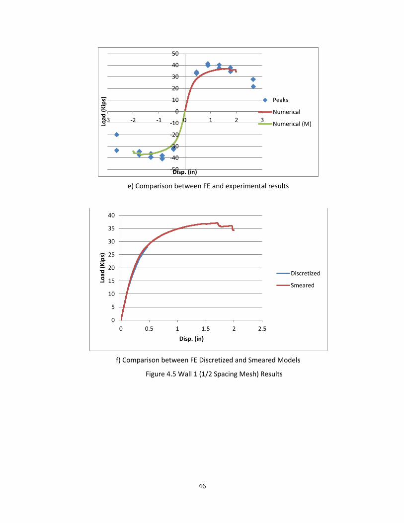
46
e) Comparison between FE and experimental results
f) Comparison between FE Discretized and Smeared Models
Figure 4.5 Wall 1 (1/2 Spacing Mesh) Results
-50
-40
-30
-20
-10
0
10
20
30
40
50
-3 -2 -1 0 1 2 3
Load
(K
ips)
Disp. (in)
Peaks
Numerical
Numerical (M)
0
5
10
15
20
25
30
35
40
0 0.5 1 1.5 2 2.5
Load
(K
ips)
Disp. (in)
Discretized
Smeared

47
a) Deflected Shape and Crack Pattern b) Masonry Principal Stresses
c) Steel Plastic Strain
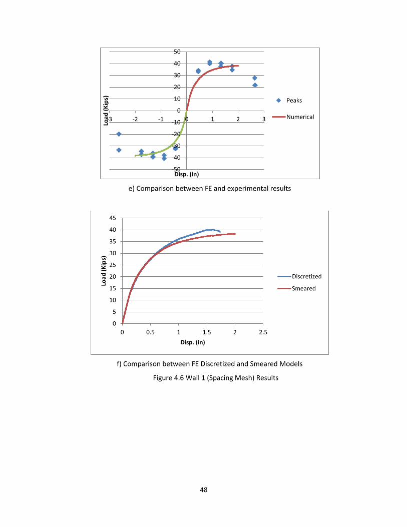
48
e) Comparison between FE and experimental results
f) Comparison between FE Discretized and Smeared Models
Figure 4.6 Wall 1 (Spacing Mesh) Results
-50
-40
-30
-20
-10
0
10
20
30
40
50
-3 -2 -1 0 1 2 3
Load
(K
ips)
Disp. (in)
Peaks
Numerical
0
5
10
15
20
25
30
35
40
45
0 0.5 1 1.5 2 2.5
Load
(K
ips)
Disp. (in)
Discretized
Smeared

49
4.5.2 Results for Specimen 8
Figures 4.7, 4.8, and 4.9 and show the results for Specimen 8 and three levels of mesh
refinement. The results of this smeared model are compared with the results of the alternative
discretized model.
The crack pattern shows smeared diagonal cracks, which represents the formation of the
strut and tie mechanism as with the discretized model. Also, due to the presence of bending,
another smeared crack pattern exists at the base. The formation of this crack pattern is related to
the amount of axial load applied to the wall. For higher values of axial load, this crack pattern will
be reduced.
Again, a localized crack appeared in the model with the finest mesh, which led to a
breakdown in the solution. With the coarser meshes, the plastic deformation was more highly
distributed and the solution proceeded much further. In those cases, although the load-deflection
curve is of a different shape compared to the experimental data points, it is interesting to note that
the eventual instability in the solution occurred at approximately the same displacement as physical
failure. In addition, the peak load value for the coarsest meshes, for which a peak was attained, is
close to those obtained for the experimental specimen. However, it should be noted that the
experimental data points represent peaks from cyclic loading, which may have accelerated damage
in the masonry. Specimen 8 is the wall most heavily influenced by shear and it is, therefore, most
influenced by damage in the masonry as compared with the taller walls which exhibit bending
behavior and are more highly influenced by plasticity in the steel.

50
a) Deflected Shape and Crack Pattern b) Masonry Principal Stresses
c) Steel Plastic Strain

51
e) Comparison between FE and experimental results
f) Comparison between FE Discretized and Smeared Models
Figure 4.7 Wall 8 (1/4 Spacing Mesh) Results
-80
-60
-40
-20
0
20
40
60
80
-1.5 -1 -0.5 0 0.5 1 1.5
Load
(K
ips)
Disp. (in)
Peaks
Numerical
Numerical (M)
0
10
20
30
40
50
60
70
0 0.1 0.2 0.3 0.4
Load
(K
ips)
Disp. (in)
Discretized
Smeared
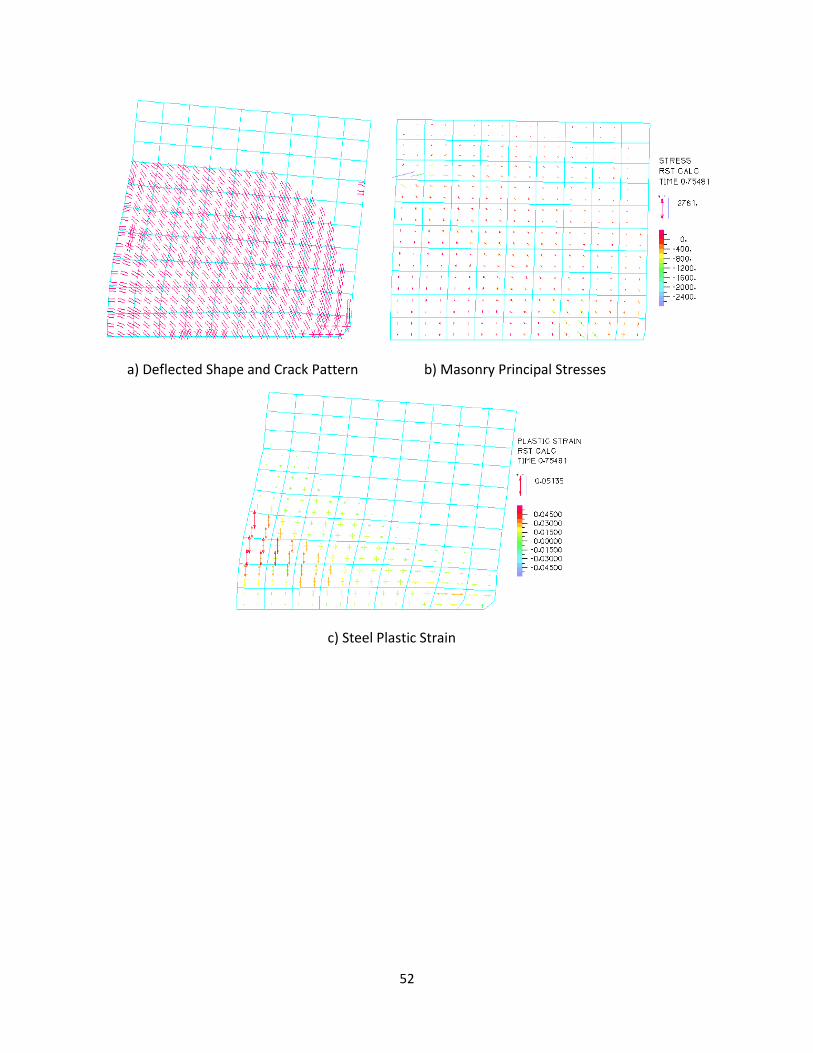
52
a) Deflected Shape and Crack Pattern b) Masonry Principal Stresses
c) Steel Plastic Strain

53
e) Comparison between FE and experimental results
f) Comparison between FE Discretized and Smeared Models
Figure 4.8 Wall 8 (1/2 Spacing Mesh) Results
-100
-80
-60
-40
-20
0
20
40
60
80
100
-2 -1 0 1 2
Load
(K
ips)
Disp. (in)
Peaks
Numerical
Numerical (M)
0
10
20
30
40
50
60
70
80
90
0 0.5 1 1.5 2
Discretized
Smeared

54
a) Deflected Shape and Crack Pattern b) Masonry Principal Stresses
c) Steel Plastic Strain

55
e) Comparison between FE and experimental results
f) Comparison between FE Discretized and Smeared Models
Figure 4.9 Wall 8 (Spacing Mesh) Results
-100
-80
-60
-40
-20
0
20
40
60
80
100
-2 -1 0 1 2
Load
(K
ips)
Disp. (in)
Peaks
Numerical
Numerical (M)
0
10
20
30
40
50
60
70
80
90
100
0 0.5 1 1.5 2
Discretized
Smeared

56
4.6 Discussion
The plots in Figures [4.4-4.9](e) show a strong correlation between results for the
discretized steel finite element model of reinforced masonry shear wall specimens and those for
the equivalent smeared steel finite element models. The plots also show that, as with the
discretized model, the smeared model is not affected by mesh size other than that coarse meshes
tend to progress further than fine meshes, especially for walls dominated by shear failure. Neither
modeling approach was able to accurately trace the descending part of the load-displacement
curve.
Again, In order to control the fictitious damping effect on the model and to predict the wall
displacement at peak load, the calculated failure load from Table 3.3 can be used. If the model was
unable to develop a peak value of load (ND), increasing the fictitious damping coefficient will allow
the solution to progress further. However, increased damping may result in unrealistic behavior. In
Table 3.5, the displacement values from the finite element models at calculated peak load are given
and compared to those from the experimental tests. The displacement associated with these loads
varies from the experimental data by 20-67%. The variance in results is higher than that of the
discretized model because smearing of the steel caused yielding of the wall to occur sooner,
resulting in higher displacement at peak load.
Table 4.2 Peak Load Displacements
Specimens
Experimental
PLD (in)
Predicted PLD (in) (Var. %)
¼ spacing mesh ½ spacing mesh Spacing mesh
1 1.1 ND 1.64 (49.1) 1.44 (30.9)
2 0.55 ND 0.84 (52.7) 0.7 (27.3)
3 0.7 0.26 (62.8) 0.41 (41.4) 0.4 (42.9)
4 0.59 0.79 (33.9) 0.98 (66.1) ND
5 0.57 ND 0.88 (54.4) 0.73 (28.1)
6 0.95 ND 1.25 (31.6) 1.15 (21.1)
7 0.89 ND ND ND
8 0.27 ND 0.45 (66.7) 0.43 (59.3)

57
The equivalent smeared models were better able to overcome the numerical difficulties
exhibited by the discretized models for the shear dominated wall specimens. This is likely because,
for the former, all finite elements were influenced by the reinforcement and the effect of masonry
cracking was distributed. For the latter, masonry elements without discrete bars experienced a
large reduction in stress capacity and stiffness when they cracked, which led to an early numerical
breakdown of the solution.
Although detailed steel/masonry interaction is beyond the simulation capability of the
smeared model, the general crack pattern and steel yielding zones were accurately depicted with
much less time required for model preparation and computer execution than for the discrete
model.
58
CHAPTER FIVE
SUMMARY AND CONCLUSIONS
5.1 Summary
Scaling techniques for the constitutive relations of reinforced masonry shear walls to
account for initial cracking were developed to simplify the construction of finite element models for
their analysis. These techniques provide solutions for macro modeling of these walls that are valid
up to the point of yielding of the reinforcement or gross cracking of the masonry.
For considering the macro scale modeling of reinforced masonry walls beyond the elastic
range, the masonry was assumed to have constitutive relations of a similar form to those of
concrete at the macro level. Full nonlinear masonry constitutive relations were obtained by scaling,
in terms of strains, concrete relations with the ratio of their initial moduli of elasticity.
Steel reinforcement was smeared in an orthotropic element, with properties obtained from
stress scaling of the original steel layout, to represent the different reinforcement ratios in both
horizontal and vertical directions. This element, including plastic deformation, was overlaid on an
identical masonry element.
When compared with experimental results and more detailed finite element results, models
composed of the proposed elements showed good agreement with regard to initial cracked
stiffness and peak load capacity, when it was attained. The deformation of shear wall specimens at
failure was estimated by evaluating displacement at the peak load indicated by existing LRFD design
provisions. The values predicted by the discretized models were within experimental accuracy,
while those from the smeared models over predicted displacement at peak load due to premature
yielding of the steel. Their behavior was insensitive to mesh size and consistent results were
obtained for meshes that were relatively coarse. They successfully predicted the performance of
walls with various aspect ratios, steel reinforcement patterns, and axial load.
Finally, it is important to mention that both models require using fictitious dynamics with
them in order to overcome the instability that results from cracking. This damping does not have an
effect on the load-displacement path, but it does give the model the ability to progress further with
load/displacement. However, even the fictitious damping did not enable the model to predict the
descending part of the load-displacement behavior.

59
5.2 Conclusions
The proposed simplified modeling techniques appear to be adequate to reduce model
construction and solution time. The discretized steel model shows significant ability to predict
masonry shear wall behavior, even with very coarse meshing. The smeared steel model provided
similar results and was more robust than the discretized steel model in spite of the fact that it only
required a fraction of the detailing effort and solution time. Also, the proposed masonry
constitutive relationship, based on strain scaling of a standard concrete model, was shown to be a
good representation for the macro behavior of masonry.
This simplified representation of masonry shear walls can be used as a part of a full building
model. Most practicing engineers should have the ability to use these models to examine the wall
behavior, as a part of the entire structure, and check their design. Also, they need only the masonry
prism compressive stress and steel design stress properties to set up the material constitutive
relations.
Both models are capable of predicting masonry shear wall behavior for relatively long or
short walls, even with relatively coarse meshes. Compared with experimental tests, they were
shown to be able to represent both flexural and shear response, with and without the effect of axial
load. These features make them more appropriate for nonlinear analysis than ordinary or deep
beam theories.
The biggest limitation to widespread use of this element for masonry shear wall analysis
may be the capabilities required of the finite element software. A full nonlinear failure analysis
requires a multidimensional concrete constitutive model, an elastio-plastic orthotropic material
model, and some means to progress beyond initial localized cracking. For other, more basic
software, the initial masonry modulus of elasticity could be used with the steel elastic modulus to
simulate stiffness and approximately estimate the behavior prior to steel yielding or gross masonry
cracking.
5.3 Further Research
The scope of this research was on static nonlinear analysis. More research is required to
develop these techniques for cyclic loading or nonlinear dynamic analysis. The developed
techniques in this research are based on estimating the effective stiffness for a targeted loading

60
point, which is not the same for the suggested further research. It may require a variable material
constitutive relation scaling to be applied at each cycle.
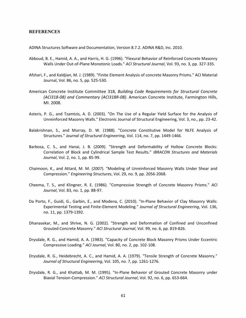
61
REFERENCES
ADINA Structures Software and Documentation, Version 8.7.2. ADINA R&D, Inc. 2010.
Abboud, B. E., Hamid, A. A., and Harris, H. G. (1996). "Flexural Behavior of Reinforced Concrete Masonry Walls Under Out-of-Plane Monotonic Loads." ACI Structural Journal, Vol. 93, no. 3, pp. 327-335.
Afshari, F., and Kaldjian, M. J. (1989). "Finite Element Analysis of concrete Masonry Prisms." ACI Material Journal, Vol. 86, no. 5, pp. 525-530.
American Concrete Institute Committee 318, Building Code Requirements for Structural Concrete (ACI318-08) and Commentary (ACI318R-08). American Concrete Institute, Farmington Hills, MI. 2008.
Asteris, P. G., and Tzamtzis, A. D. (2003). "On The Use of a Regular Yield Surface for the Analysis of Unreinforced Masonry Walls." Electronic Journal of Structural Engineering, Vol. 3, no., pp. 23-42.
Balakrishnan, S., and Murray, D. W. (1988). "Concrete Constitutive Model for NLFE Analysis of Structures." Journal of Structural Engineering, Vol. 114, no. 7, pp. 1449-1466.
Barbosa, C. S., and Hanai, J. B. (2009). "Strength and Deformability of Hollow Concrete Blocks: Correlation of Block and Cylindrical Sample Test Results." IBRACON Structures and Materials Journal, Vol. 2, no. 1, pp. 85-99.
Chaimoon, K., and Attard, M. M. (2007). "Modeling of Unreinforced Masonry Walls Under Shear and Compression." Engineering Structures, Vol. 29, no. 9, pp. 2056-2068.
Cheema, T. S., and Klingner, R. E. (1986). "Compressive Strength of Concrete Masonry Prisms." ACI Journal, Vol. 83, no. 1, pp. 88-97.
Da Porto, F., Guidi, G., Garbin, E., and Modena, C. (2010). "In-Plane Behavior of Clay Masonry Walls: Experimental Testing and Finite-Element Modeling." Journal of Structural Engineering, Vol. 136, no. 11, pp. 1379-1392.
Dhanasekar, M., and Shrive, N. G. (2002). "Strength and Deformation of Confined and Unconfined Grouted Concrete Masonry." ACI Structural Journal, Vol. 99, no. 6, pp. 819-826.
Drysdale, R. G., and Hamid, A. A. (1983). "Capacity of Concrete Block Masonry Prisms Under Eccentric Compressive Loading." ACI Journal, Vol. 80, no. 2, pp. 102-108.
Drysdale, R. G., Heidebrecht, A. C., and Hamid, A. A. (1979). "Tensile Strength of Concrete Masonry." Journal of Structural Engineering, Vol. 105, no. 7, pp. 1261-1276.
Drysdale, R. G., and Khattab, M. M. (1995). "In-Plane Behavior of Grouted Concrete Masonry under Biaxial Tension-Compression." ACI Structural Journal, Vol. 92, no. 6, pp. 653-664.
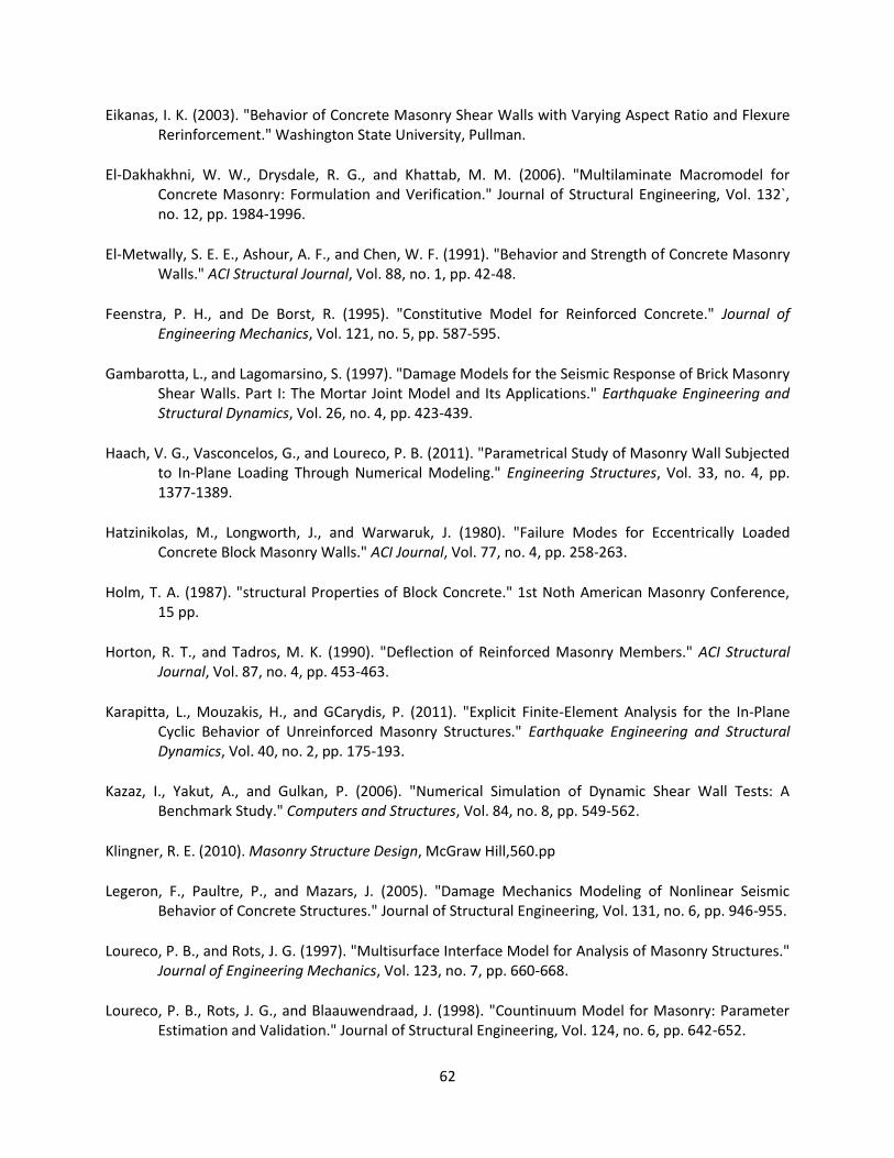
62
Eikanas, I. K. (2003). "Behavior of Concrete Masonry Shear Walls with Varying Aspect Ratio and Flexure Rerinforcement." Washington State University, Pullman.
El-Dakhakhni, W. W., Drysdale, R. G., and Khattab, M. M. (2006). "Multilaminate Macromodel for Concrete Masonry: Formulation and Verification." Journal of Structural Engineering, Vol. 132`, no. 12, pp. 1984-1996.
El-Metwally, S. E. E., Ashour, A. F., and Chen, W. F. (1991). "Behavior and Strength of Concrete Masonry Walls." ACI Structural Journal, Vol. 88, no. 1, pp. 42-48.
Feenstra, P. H., and De Borst, R. (1995). "Constitutive Model for Reinforced Concrete." Journal of Engineering Mechanics, Vol. 121, no. 5, pp. 587-595.
Gambarotta, L., and Lagomarsino, S. (1997). "Damage Models for the Seismic Response of Brick Masonry Shear Walls. Part I: The Mortar Joint Model and Its Applications." Earthquake Engineering and Structural Dynamics, Vol. 26, no. 4, pp. 423-439.
Haach, V. G., Vasconcelos, G., and Loureco, P. B. (2011). "Parametrical Study of Masonry Wall Subjected to In-Plane Loading Through Numerical Modeling." Engineering Structures, Vol. 33, no. 4, pp. 1377-1389.
Hatzinikolas, M., Longworth, J., and Warwaruk, J. (1980). "Failure Modes for Eccentrically Loaded Concrete Block Masonry Walls." ACI Journal, Vol. 77, no. 4, pp. 258-263.
Holm, T. A. (1987). "structural Properties of Block Concrete." 1st Noth American Masonry Conference, 15 pp.
Horton, R. T., and Tadros, M. K. (1990). "Deflection of Reinforced Masonry Members." ACI Structural Journal, Vol. 87, no. 4, pp. 453-463.
Karapitta, L., Mouzakis, H., and GCarydis, P. (2011). "Explicit Finite-Element Analysis for the In-Plane Cyclic Behavior of Unreinforced Masonry Structures." Earthquake Engineering and Structural Dynamics, Vol. 40, no. 2, pp. 175-193.
Kazaz, I., Yakut, A., and Gulkan, P. (2006). "Numerical Simulation of Dynamic Shear Wall Tests: A Benchmark Study." Computers and Structures, Vol. 84, no. 8, pp. 549-562.
Klingner, R. E. (2010). Masonry Structure Design, McGraw Hill,560.pp
Legeron, F., Paultre, P., and Mazars, J. (2005). "Damage Mechanics Modeling of Nonlinear Seismic Behavior of Concrete Structures." Journal of Structural Engineering, Vol. 131, no. 6, pp. 946-955.
Loureco, P. B., and Rots, J. G. (1997). "Multisurface Interface Model for Analysis of Masonry Structures." Journal of Engineering Mechanics, Vol. 123, no. 7, pp. 660-668.
Loureco, P. B., Rots, J. G., and Blaauwendraad, J. (1998). "Countinuum Model for Masonry: Parameter Estimation and Validation." Journal of Structural Engineering, Vol. 124, no. 6, pp. 642-652.

63
Mojsilovic, N., and Marti, P. (1997). "Strength of Masonry Subjected to Combined Actions." ACI Structural Journal, Vol. 96, no. 4, pp. 633-640.
Nilson, A. H. (1987). Design of Prestressed Concrete, 2nd edition. Wiley, New York,592.pp
Nilson, A. H., Darwin, D., and Dolan, C. W. (2003). Design of Concrete Structures, 14th Edition. McGraw Hill,795.pp
Priestley, M. J. N. (1986). "Seismic Design of Concrete Masonry Shearwalls." ACI Structural Journal, Vol. 83, no. 1, pp. 58-68.
Priestley, M. J. N., and Elder, D. M. (1983). "Stress-Strain Curves for Unconfined and Confined Concrete Masonry." ACI Journal, Vol. 80, no. 3, pp. 192-201.
Ramamurthy, K., Sathish, V., and Ambalavanan, R. (2000). "Compressive Strength Prediction of Hollow Concrete Block Masonry Prisms." ACI Structural Journal, Vol. 97, no. 1, pp. 61-67.
Selby, R. G., and Vecchio, F. J. (1997). "A Constitutive Model For Analysis of Reinforced Concrete Solids." Canadian Journal of Civil Engineering Vol. 24, no., pp. 460-470.
Sherman, J. (2011). "Effects of Key Parameters on The Performance of Concrete Masonry Shear Walls Under In-Plane Loading." Washington State University, Pullman.
Shing, P. B., Schuller, M., Hoskere, V. S., and Carter, E. (1990). "Flexural and Shear Response of Reinforced Masonry Walls." ACI Structural Journal, Vol. 87, no. 6, pp. 646-656.
Stavridis, A., and Shing, P. B. (2010). "Finite-Element Modeling of Nonlinear Behavior of Masonry-Infilled RC Frames." Journal of Structural Engineering, Vol. 136, no. 3, pp. 285-296.
Sutcliffe, D. J., Yu, H. S., and Page, A. W. (2001). "Lower Bound Limit Analysis of Unreinforced Masonry Shear Walls." Computers and Structures, Vol. 79, no. 14, pp. 1295-1312.
Vecchio, F. J. (1990). "Reinforced Concrete Membrane Element Formulations." Journal of Structural Engineering, Vol. 116, no. 3, pp. 730-750.
Vecchio, F. J., and Collins, M. P. (1986). "The Modified Compression-Field Theory for Reinforced Concrete Elements Subjected to Shear." ACI Journal, Vol. 83, no. 2, pp. 219-231.
Vecchio, F. J., and Selby, R. G. (1991). "Toward Compression-Field Analysis of Reinforced Concrete Solids." Journal of Structural Engineering, Vol. 117, no. 20, pp. 1740-1758.
Yamaguchi, E., and Ohta, T. (1993). "Accurate and Efficient Method for Analysis of Reinforced Concrete Structures." Journal of Structural Engineering, Vol. 119, no. 30, pp. 2017-2034.

64
APPENDIX A
A.1 Discretized Model Results
a) Deflected Shape and Crack Pattern b) Masonry Principal Stresses
c) Axial Strain in Steel
d) Comparison between FE and experimental results
Figure A1.1 Wall 1 (1/4 Spacing Mesh) Results
-50
-40
-30
-20
-10
0
10
20
30
40
50
-3 -2 -1 0 1 2 3
Load
(K
ips)
Disp. (in)
Peaks
Numerical
Numerical (M)

65
a) Deflected Shape and Crack Pattern b) Masonry Principal Stresses
c) Axial Strain in Steel
d) Comparison between FE and experimental results
Figure A1.2 Wall 1 (1/2 Spacing Mesh) Results
-50
-40
-30
-20
-10
0
10
20
30
40
50
-4 -2 0 2 4
Load
(K
ips)
Disp. (in)
Peaks
Numerical
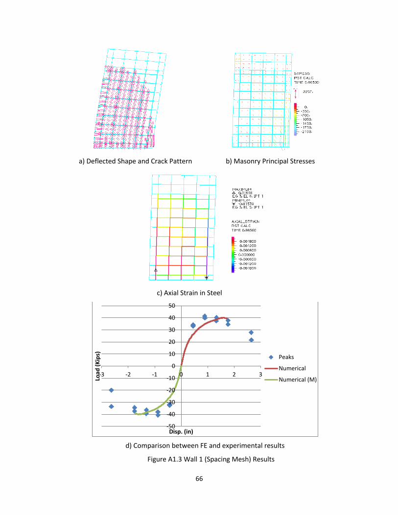
66
a) Deflected Shape and Crack Pattern b) Masonry Principal Stresses
c) Axial Strain in Steel
d) Comparison between FE and experimental results
Figure A1.3 Wall 1 (Spacing Mesh) Results
-50
-40
-30
-20
-10
0
10
20
30
40
50
-3 -2 -1 0 1 2 3
Load
(K
ips)
Disp. (in)
Peaks
Numerical
Numerical (M)

67
a) Deflected Shape and Cracks Pattern b) Masonry Principal Stresses
c) Axial Strain in Steel
d) Comparison between FE and experimental results
Figure A1.4 Wall 2 (1/4 Spacing Mesh) Results
-50
-40
-30
-20
-10
0
10
20
30
40
50
-2 -1 0 1 2
Load
(K
ips)
Disp. (in)
Peaks
Numerical
Numerical (M)

68
a) Deflected Shape and Cracks Pattern b) Masonry Principal Stresses
c) Axial Strain in Steel
d) Comparison between FE and experimental results
Figure A1.5 Wall 2 (1/2 Spacing Mesh) Results
-50
-40
-30
-20
-10
0
10
20
30
40
50
-2 -1 0 1 2 Load
(in
)
Disp. (in)
Peaks
Numerical
Numerical (M)

69
a) Deflected Shape and Crack Pattern b) Masonry Principal Stresses
c) Axial Strain in Steel
d) Comparison between FE and experimental results
Figure A1.6 Wall 2 (Spacing Mesh) Results
-50
-40
-30
-20
-10
0
10
20
30
40
50
-2 -1 0 1 2
Load
(K
ips)
Disp. (in)
Peaks
Numerical
Numerical (M)

70
a) Deflected Shape and Crack Pattern b) Masonry Principal Stresses
c) Axial Strain in Steel
d) Comparison between FE and experimental results
Figure A1.7 Wall 3 (1/4 Spacing Mesh) Results
-60
-40
-20
0
20
40
60
-1.5 -1 -0.5 0 0.5 1 1.5
Load
(K
ips)
Displ (in)
Peaks
Numerical
Numerical (M)
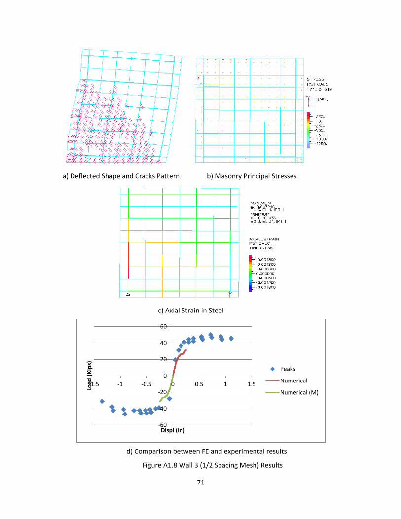
71
a) Deflected Shape and Cracks Pattern b) Masonry Principal Stresses
c) Axial Strain in Steel
d) Comparison between FE and experimental results
Figure A1.8 Wall 3 (1/2 Spacing Mesh) Results
-60
-40
-20
0
20
40
60
-1.5 -1 -0.5 0 0.5 1 1.5
Load
(K
ips)
Displ (in)
Peaks
Numerical
Numerical (M)

72
a) Deflected Shape and Crack Pattern b) Masonry Principal Stresses
c) Axial Strain in Steel
d) Comparison between FE and experimental results
Figure A1.9 Wall 3 (Spacing Mesh) Results
-80
-60
-40
-20
0
20
40
60
80
-3 -2 -1 0 1 2 3
Load
(K
ips)
Displ (in)
Peaks
Numerical
Numerical (M)

73
a) Deflected Shape and Crack Pattern b) Masonry Principal Stresses
c) Axial Strain in Steel
d) Comparison between FE and experimental results
Figure A1.10 Wall 4 (1/4 Spacing Mesh) Results
-40
-30
-20
-10
0
10
20
30
40
-3 -2 -1 0 1 2 3
Load
(K
ips)
Disp. (in)
Peaks
Numerical
Numerical (M)
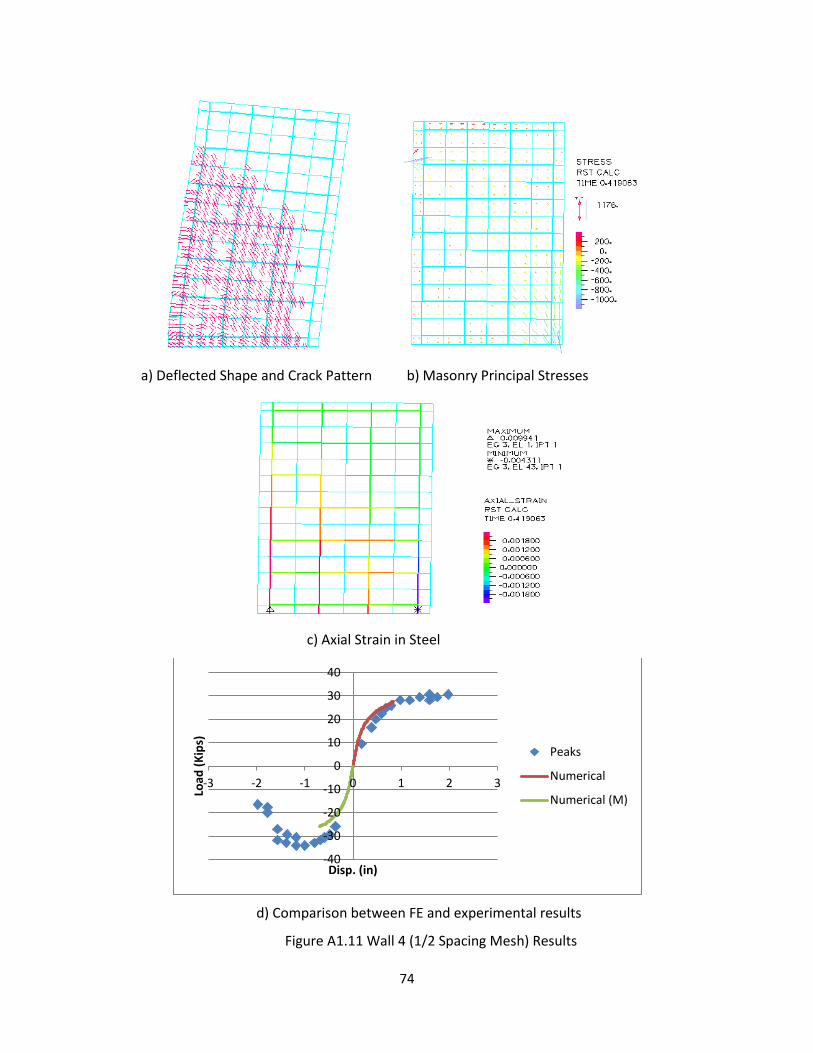
74
a) Deflected Shape and Crack Pattern b) Masonry Principal Stresses
c) Axial Strain in Steel
d) Comparison between FE and experimental results
Figure A1.11 Wall 4 (1/2 Spacing Mesh) Results
-40
-30
-20
-10
0
10
20
30
40
-3 -2 -1 0 1 2 3
Load
(K
ips)
Disp. (in)
Peaks
Numerical
Numerical (M)

75
a) Deflected Shape and Crack Pattern b) Masonry Principal Stresses
c) Axial Strain in Steel
d) Comparison between FE and experimental results
Figure A1.12 Wall 4 (Spacing Mesh) Results
-40
-30
-20
-10
0
10
20
30
40
-3 -2 -1 0 1 2 3
Load
(K
ips)
Disp. (in)
Peaks
Numerical
Numerical (M)

76
a) Deflected Shape and Crack Pattern b) Masonry Principal Stresses
c) Axial Strain in Steel
d) Comparison between FE and experimental results
Figure A1.13 Wall 5 (1/4 Spacing Mesh) Results
-60
-40
-20
0
20
40
60
80
-2 -1 0 1 2 Load
(K
ips)
Disp. (in)
Peaks
Numerical
Numerical (M)

77
a) Deflected Shape and Crack Pattern b) Masonry Principal Stresses
c) Axial Strain in Steel
d) Comparison between FE and experimental results
Figure A1.14 Wall 5 (1/2 Spacing Mesh) Results
-60
-40
-20
0
20
40
60
80
-2 -1 0 1 2 Load
(K
ips)
Disp. (in)
Peaks
Numerical
Numerical (M)

78
a) Deflected Shape and Crack Pattern b) Masonry Principal Stresses
c) Axial Strain in Steel
d) Comparison between FE and experimental results
Figure A1.15 Wall 5 (Spacing Mesh) Results
-60
-40
-20
0
20
40
60
80
-2 -1 0 1 2 Load
(K
ips)
Disp. (in)
Peaks
Numerical
Numerical (M)

79
a) Deflected Shape and Crack Pattern b) Masonry Principal Stresses
c) Axial Strain in Steel
d) Comparison between FE and experimental results
Figure A1.16 Wall 6 (1/4 Spacing Mesh) Results
-60
-40
-20
0
20
40
60
-3 -2 -1 0 1 2 3
Load
(K
ips)
Disp. (in)
Peaks
Numerical
Numerical (M)

80
a) Deflected Shape and Crack Pattern b) Masonry Principal Stresses
c) Axial Strain in Steel
d) Comparison between FE and experimental results
Figure A1.17 Wall 6 (1/2 Spacing Mesh) Results
-60
-40
-20
0
20
40
60
-3 -2 -1 0 1 2 3
Load
(K
ips)
Disp. (in)
Peaks
Numerical
Numerical (M)

81
a) Deflected Shape and Crack Pattern b) Masonry Principal Stresses
c) Axial Strain in Steel
d) Comparison between FE and experimental results
Figure A1.18 Wall 6 (Spacing Mesh) Results
-50
-40
-30
-20
-10
0
10
20
30
40
50
60
-3 -2 -1 0 1 2 3 Load
(K
ips)
Disp. (in)
Peaks
Numerical
Numerical (M)

82
a) Deflected Shape and Crack Pattern b) Masonry Principal Stresses
c) Axial Strains in Steel
d) Comparison between FE and experimental results
Figure A1.19 Wall 7 (1/4 Spacing Mesh) Results
-30
-20
-10
0
10
20
30
-3 -2 -1 0 1 2 3
Load
(K
ips)
Disp. (in)
Peaks
Numerical
Numerical (M)

83
a) Deflected Shape and Crack Pattern b) Masonry Principal Stresses
c) Axial Strains in Steel
d) Comparison between FE and experimental results
Figure A1.20 Wall 7 (1/2 Spacing Mesh) Results
-30
-20
-10
0
10
20
30
-3 -2 -1 0 1 2 3
Load
(K
ips)
Disp. (in)
Peaks
Numerical
Numerical (M)

84
a) Deflected Shape and Crack Pattern b) Masonry Principal Stresses
c) Axial Strains in Steel
d) Comparison between FE and experimental results
Figure A1.21 Wall 7 (Spacing Mesh) Results
-30
-20
-10
0
10
20
30
-3 -2 -1 0 1 2 3
Load
(K
ips)
Disp. (in)
Peaks
Numerical
Numerical (M)

85
a) Deflected Shape and Crack Pattern b) Masonry Principal Stresses
c) Axial Strains in Steel
d) Comparison between FE and experimental results
Figure A1.22 Wall 8 (1/4 Spacing Mesh) Results
-80
-60
-40
-20
0
20
40
60
80
-1.5 -1 -0.5 0 0.5 1 1.5
Load
(K
ips)
Disp. (in)
Peaks
Numerical
Numerical (M)

86
a) Deflected Shape and Crack Pattern b) Masonry Principal Stresses
c) Axial Strains in Steel
d) Comparison between FE and experimental results
Figure A1.23 Wall 8 (1/2 Spacing Mesh) Results
-80
-60
-40
-20
0
20
40
60
80
-1.5 -1 -0.5 0 0.5 1 1.5
Load
(K
ips)
Disp. (in)
Peaks
Numerical
Numerical (M)
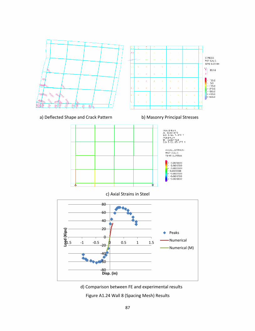
87
a) Deflected Shape and Crack Pattern b) Masonry Principal Stresses
c) Axial Strains in Steel
d) Comparison between FE and experimental results
Figure A1.24 Wall 8 (Spacing Mesh) Results
-80
-60
-40
-20
0
20
40
60
80
-1.5 -1 -0.5 0 0.5 1 1.5
Load
(K
ips)
Disp. (in)
Peaks
Numerical
Numerical (M)

88
A.2 Smeared Model Results
a) Deflected Shape and Crack Pattern b) Masonry Principal Stresses
c) Steel Plastic Strain

89
e) Comparison between FE and experimental results
f) Comparison between FE Discretized and Smeared Models
Figure A2.1 Wall 1 (1/4 Spacing Mesh) Results
-50
-40
-30
-20
-10
0
10
20
30
40
50
-3 -2 -1 0 1 2 3
Load
(K
ips)
Disp. (in)
Peaks
Numerical
Numerical (M)
0
5
10
15
20
25
30
35
40
0 0.2 0.4 0.6 0.8 1
Load
(K
ips)
Disp. (in)
Discretized
Smeared

90
a) Deflected Shape and Crack Pattern b) Masonry Principal Stresses
c) Steel Plastic Strain

91
e) Comparison between FE and experimental results
f) Comparison between FE Discretized and Smeared Models
Figure A2.2 Wall 1 (1/2 Spacing Mesh) Results
-50
-40
-30
-20
-10
0
10
20
30
40
50
-3 -2 -1 0 1 2 3
Load
(K
ips)
Disp. (in)
Peaks
Numerical
Numerical (M)
0
5
10
15
20
25
30
35
40
0 0.5 1 1.5 2 2.5
Load
(K
ips)
Disp. (in)
Discretized
Smeared

92
a) Deflected Shape and Crack Pattern b) Masonry Principal Stresses
c) Steel Plastic Strain
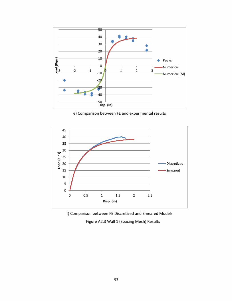
93
e) Comparison between FE and experimental results
f) Comparison between FE Discretized and Smeared Models
Figure A2.3 Wall 1 (Spacing Mesh) Results
-50
-40
-30
-20
-10
0
10
20
30
40
50
-3 -2 -1 0 1 2 3
Load
(K
ips)
Disp. (in)
Peaks
Numerical
Numerical (M)
0
5
10
15
20
25
30
35
40
45
0 0.5 1 1.5 2 2.5
Load
(K
ips)
Disp. (in)
Discretized
Smeared

94
a) Deflected Shape and Crack Pattern b) Masonry Principal Stresses
.
c) Steel Plastic Strain

95
e) Comparison between FE and experimental results
f) Comparison between FE Discretized and Smeared Models
Figure A2.4 Wall 2 (1/4 Spacing Mesh) Results
-50
-40
-30
-20
-10
0
10
20
30
40
50
-2 -1 0 1 2
Load
(K
ips)
Disp. (in)
Peaks
Numerical
Numerical (M)
0
5
10
15
20
25
30
35
0 0.2 0.4 0.6 0.8
Load
(K
ips)
Disp. (in)
Discretized
Smeared

96
a) Deflected Shape and Crack Pattern b) Masonry Principal Stresses
c) Steel Plastic Strain

97
e) Comparison between FE and experimental results
f) Comparison between FE Discretized and Smeared Models
Figure A2.5 Wall 2 (1/2 Spacing Mesh) Results
-50
-40
-30
-20
-10
0
10
20
30
40
50
-2 -1 0 1 2 Load
(in
)
Disp. (in)
Peaks
Numerical
Numerical (M)
0
5
10
15
20
25
30
35
0 0.2 0.4 0.6 0.8 1 1.2
Load
(K
ips)
Disp. (in)
Discretized
Smeared
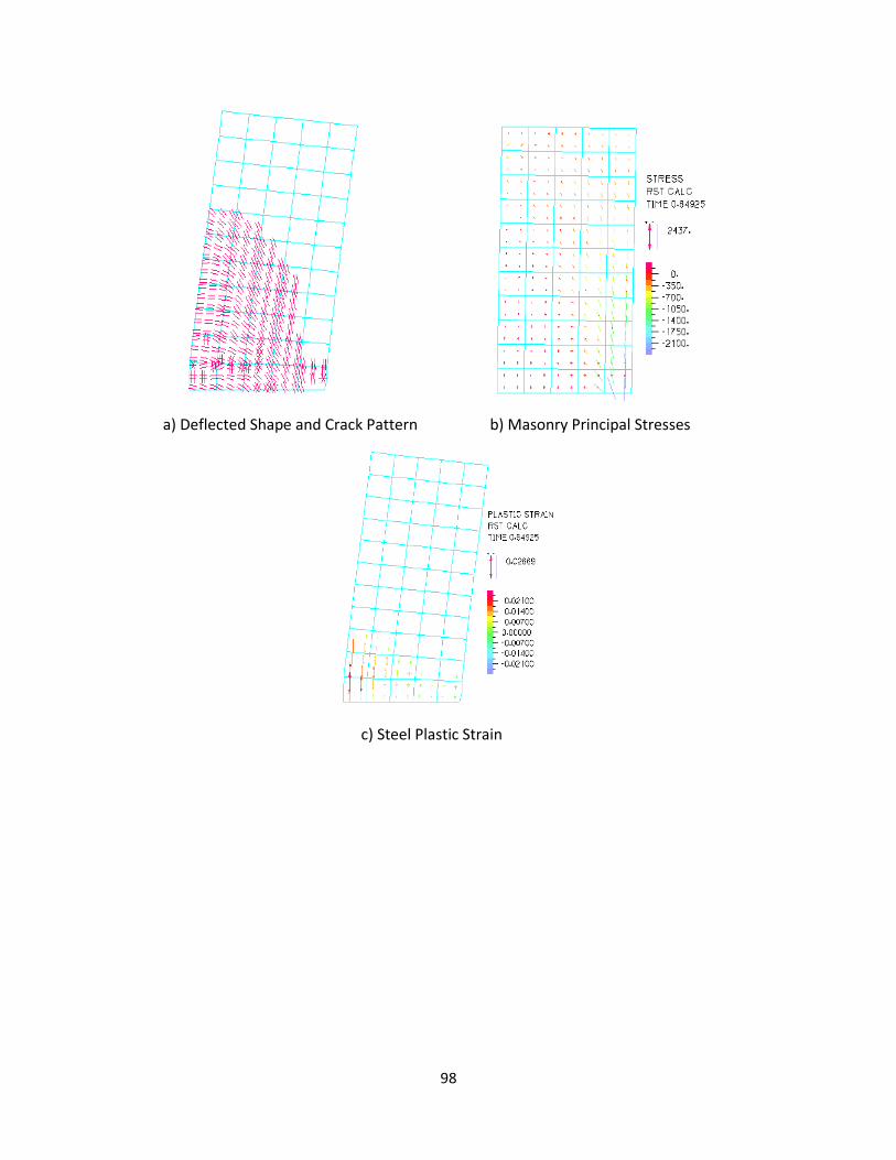
98
a) Deflected Shape and Crack Pattern b) Masonry Principal Stresses
c) Steel Plastic Strain
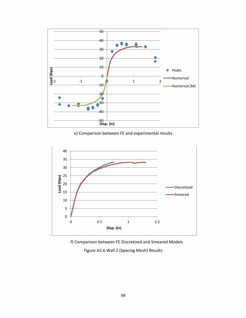
99
e) Comparison between FE and experimental results
.
f) Comparison between FE Discretized and Smeared Models
Figure A2.6 Wall 2 (Spacing Mesh) Results
-50
-40
-30
-20
-10
0
10
20
30
40
50
-2 -1 0 1 2
Load
(K
ips)
Disp. (in)
Peaks
Numerical
Numerical (M)
0
5
10
15
20
25
30
35
40
0 0.5 1 1.5
Load
(K
ips)
Disp. (in)
Discretized
Smeared

100
a) Deflected Shape and Crack Pattern b) Masonry Principal Stresses
c) Steel Plastic Strain

101
e) Comparison between FE and experimental results
f) Comparison between FE Discretized and Smeared Models
Figure A2.7 Wall 3 (1/4 Spacing Mesh) Results
-100
-80
-60
-40
-20
0
20
40
60
80
100
-1.5 -1 -0.5 0 0.5 1 1.5
Load
(K
ips)
Displ (in)
Peaks
Numerical
Numerical (M)
0
10
20
30
40
50
60
70
80
90
0 0.5 1 1.5
Load
(K
ips)
Disp. (in)
Discretized
Smeared
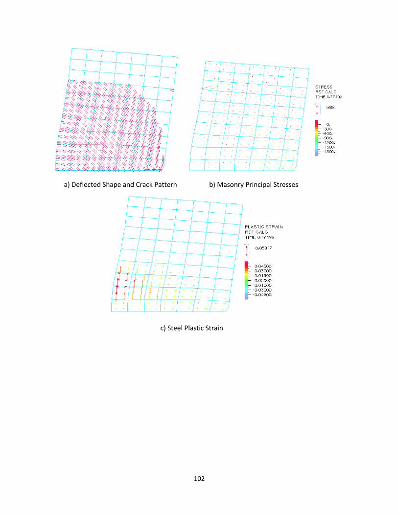
102
a) Deflected Shape and Crack Pattern b) Masonry Principal Stresses
c) Steel Plastic Strain
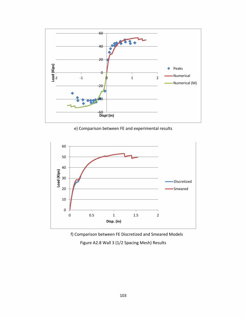
103
e) Comparison between FE and experimental results
f) Comparison between FE Discretized and Smeared Models
Figure A2.8 Wall 3 (1/2 Spacing Mesh) Results
-60
-40
-20
0
20
40
60
-2 -1 0 1 2
Load
(K
ips)
Displ (in)
Peaks
Numerical
Numerical (M)
0
10
20
30
40
50
60
0 0.5 1 1.5 2
Load
(K
ips)
Disp. (in)
Discretized
Smeared

104
a) Deflected Shape and Crack Pattern b) Masonry Principal Stresses
c) Steel Plastic Strain

105
e) Comparison between FE and experimental results
f) Comparison between FE Discretized and Smeared Models
Figure A2.9 Wall 3 (Spacing Mesh) Results
-80
-60
-40
-20
0
20
40
60
80
-1.5 -1 -0.5 0 0.5 1 1.5
Load
(K
ips)
Displ (in)
Peaks
Numerical
Numerical (M)
0
10
20
30
40
50
60
0 0.5 1 1.5 2
Load
(K
ips)
Disp. (in)
Discretized
Smeared

106
a) Deflected Shape and Crack Pattern b) Masonry Principal Stresses
c) Steel Plastic Strain

107
e) Comparison between FE and experimental results
f) Comparison between FE Discretized and Smeared Models
Figure A2.10 Wall 4 (1/4 Spacing Mesh) Results
-40
-30
-20
-10
0
10
20
30
40
-3 -2 -1 0 1 2 3
Load
(K
ips)
Disp. (in)
Peaks
Numerical
Numerical (M)
0
5
10
15
20
25
30
35
0 0.5 1 1.5
Load
(K
ips)
Disp. (in)
Discretized
Smeared

108
a) Deflected Shape and Crack Pattern b) Masonry Principal Stresses
c) Steel Plastic Strain

109
e) Comparison between FE and experimental results
f) Comparison between FE Discretized and Smeared Models
Figure A2.11 Wall 4 (1/2 Spacing Mesh) Results
-40
-30
-20
-10
0
10
20
30
40
-3 -2 -1 0 1 2 3
Load
(K
ips)
Disp. (in)
Peaks
Numerical
Numerical (M)
0
5
10
15
20
25
30
35
0 0.5 1 1.5 2 2.5
Load
(K
ips)
Disp. (in)
Discretized
Smeared

110
a) Deflected Shape and Crack Pattern b) Masonry Principal Stresses
c) Steel Plastic Strain

111
e) Comparison between FE and experimental results
f) Comparison between FE Discretized and Smeared Models
Figure A2.12 Wall 4 (Spacing Mesh) Results
-40
-30
-20
-10
0
10
20
30
40
-3 -2 -1 0 1 2 3
Load
(K
ips)
Disp. (in)
Peaks
Numerical
Numerical (M)
0
2
4
6
8
10
12
14
16
18
20
0 0.1 0.2 0.3 0.4
Discretized
Smeared
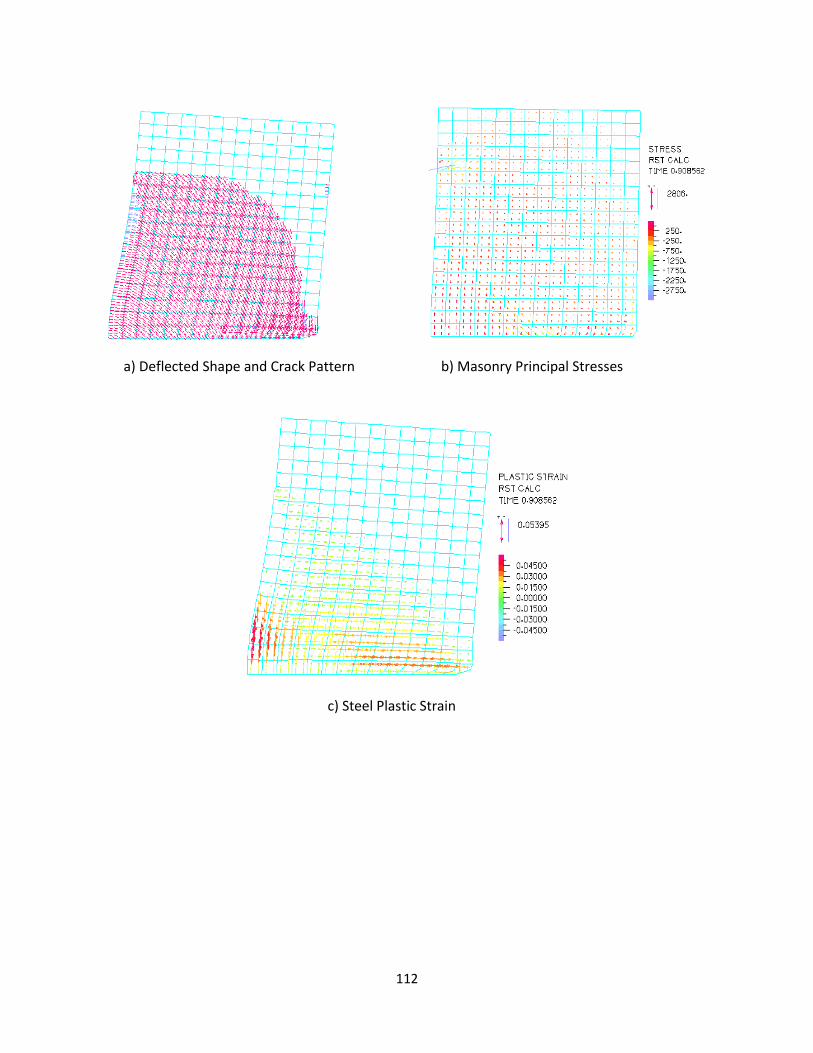
112
a) Deflected Shape and Crack Pattern b) Masonry Principal Stresses
c) Steel Plastic Strain

113
e) Comparison between FE and experimental results
f) Comparison between FE Discretized and Smeared Models
Figure A2.13 Wall 5 (1/4 Spacing Mesh) Results
-80
-60
-40
-20
0
20
40
60
80
-2 -1 0 1 2
Load
(K
ips)
Disp. (in)
Peaks
Numerical
Numerical (M)
0
10
20
30
40
50
60
70
0 0.5 1 1.5 2
Load
(K
ips)
Disp. (in)
Discretized
Smeared

114
a) Deflected Shape and Crack Pattern b) Masonry Principal Stresses
c) Steel Plastic Strain

115
e) Comparison between FE and experimental results
f) Comparison between FE Discretized and Smeared Models
Figure A2.14 Wall 5 (1/2 Spacing Mesh) Results
-80
-60
-40
-20
0
20
40
60
80
-2 -1 0 1 2
Load
(K
ips)
Disp. (in)
Peaks
Numerical
Numerical (M)
0
10
20
30
40
50
60
70
0 0.5 1 1.5
Load
(K
ips)
Disp. (in)
Discretized
Smeared
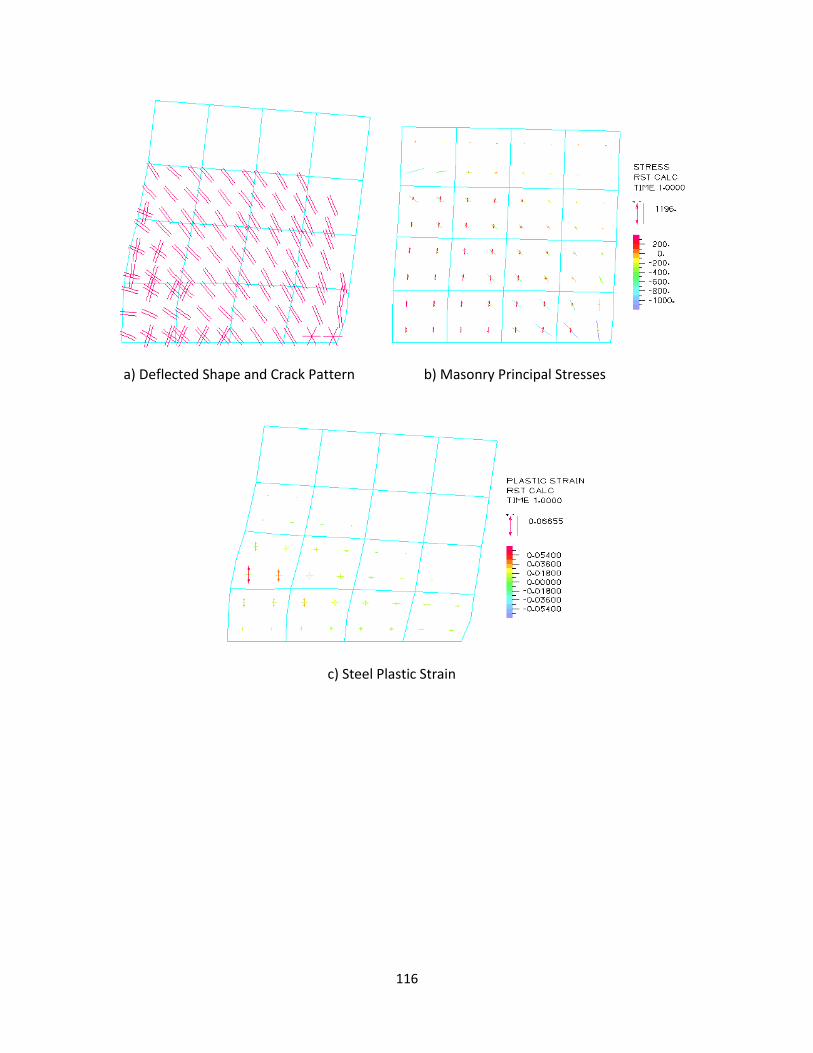
116
a) Deflected Shape and Crack Pattern b) Masonry Principal Stresses
c) Steel Plastic Strain

117
e) Comparison between FE and experimental results
f) Comparison between FE Discretized and Smeared Models
Figure A2.15 Wall 5 (Spacing Mesh) Results
-80
-60
-40
-20
0
20
40
60
80
-3 -2 -1 0 1 2 3
Load
(K
ips)
Disp. (in)
Peaks
Numerical
Numerical (M)
0
10
20
30
40
50
60
70
80
0 0.5 1 1.5 2 2.5
Load
(K
ips)
Disp. (in)
Discretized
Smeared
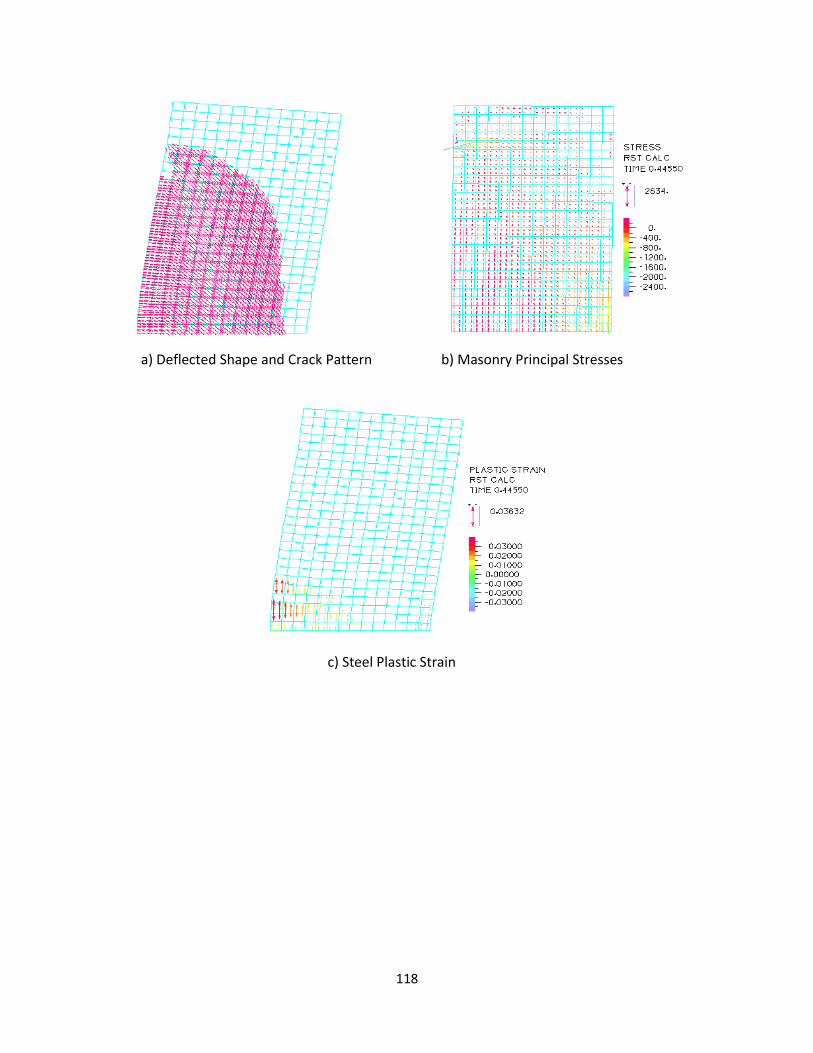
118
a) Deflected Shape and Crack Pattern b) Masonry Principal Stresses
c) Steel Plastic Strain

119
e) Comparison between FE and experimental results
f) Comparison between FE Discretized and Smeared Models
Figure A2.16 Wall 6 (1/4 Spacing Mesh) Results
-50
-40
-30
-20
-10
0
10
20
30
40
50
60
-3 -2 -1 0 1 2 3 Load
(K
ips)
Disp. (in)
Peaks
Numerical
Numerical (M)
0
5
10
15
20
25
30
35
40
0 0.2 0.4 0.6 0.8 1
Load
(K
ips)
Disp. (in)
Discretized
Smeared

120
a) Deflected Shape and Crack Pattern b) Masonry Principal Stresses
c) Steel Plastic Strain
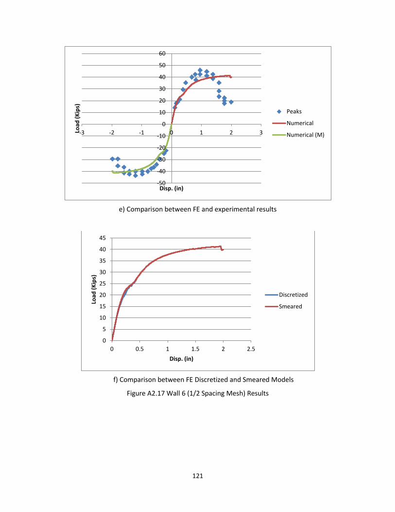
121
e) Comparison between FE and experimental results
f) Comparison between FE Discretized and Smeared Models
Figure A2.17 Wall 6 (1/2 Spacing Mesh) Results
-50
-40
-30
-20
-10
0
10
20
30
40
50
60
-3 -2 -1 0 1 2 3 Load
(K
ips)
Disp. (in)
Peaks
Numerical
Numerical (M)
0
5
10
15
20
25
30
35
40
45
0 0.5 1 1.5 2 2.5
Load
(K
ips)
Disp. (in)
Discretized
Smeared
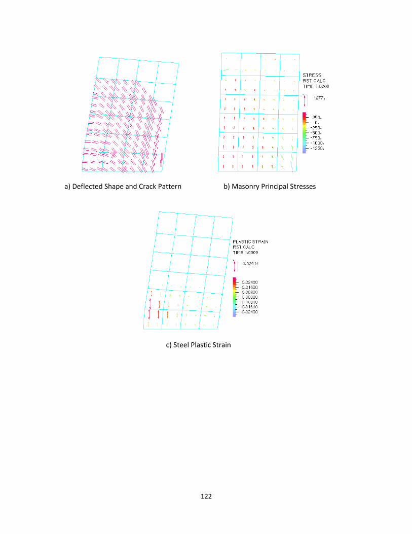
122
a) Deflected Shape and Crack Pattern b) Masonry Principal Stresses
c) Steel Plastic Strain
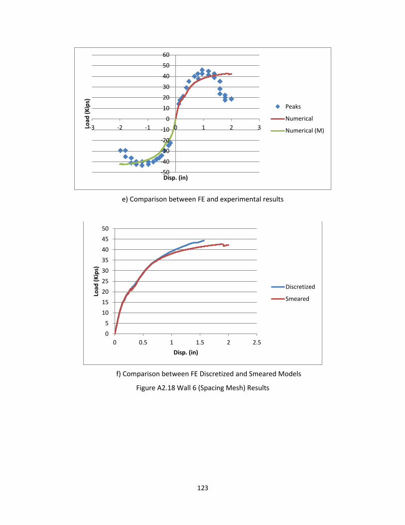
123
e) Comparison between FE and experimental results
f) Comparison between FE Discretized and Smeared Models
Figure A2.18 Wall 6 (Spacing Mesh) Results
-50
-40
-30
-20
-10
0
10
20
30
40
50
60
-3 -2 -1 0 1 2 3 Load
(K
ips)
Disp. (in)
Peaks
Numerical
Numerical (M)
0
5
10
15
20
25
30
35
40
45
50
0 0.5 1 1.5 2 2.5
Load
(K
ips)
Disp. (in)
Discretized
Smeared

124
a) Deflected Shape and Crack Pattern b) Masonry Principal Stresses
c) Steel Plastic Strain
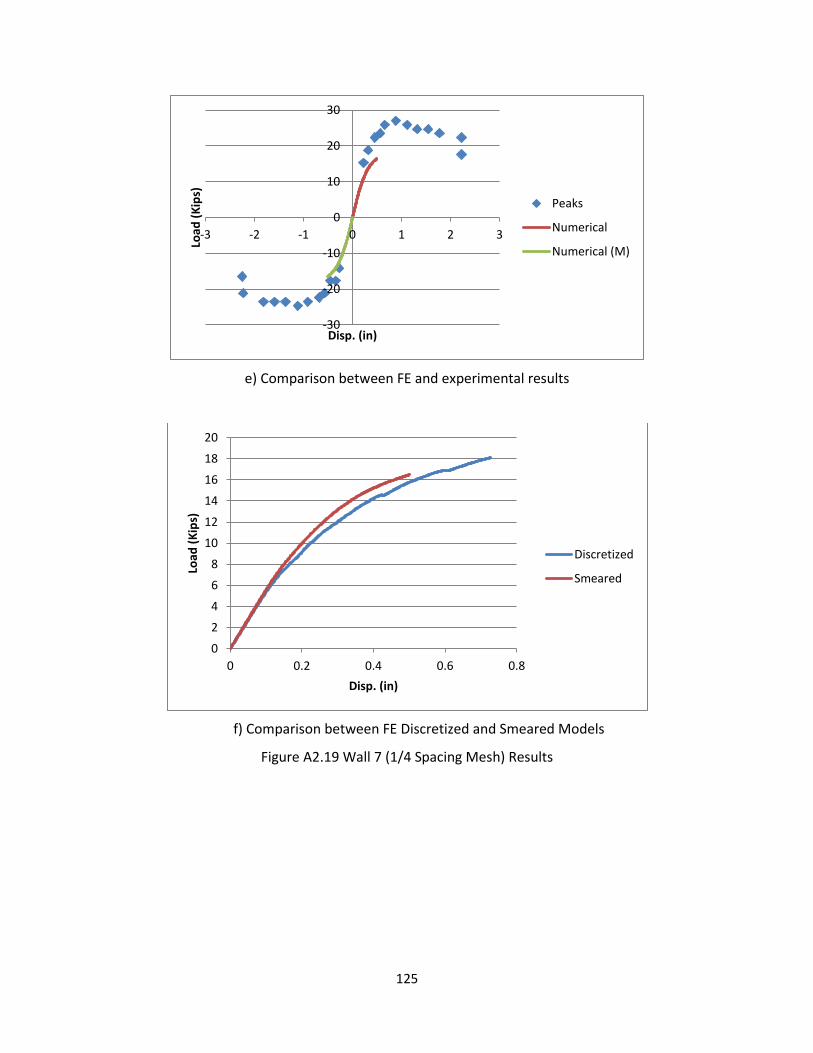
125
e) Comparison between FE and experimental results
f) Comparison between FE Discretized and Smeared Models
Figure A2.19 Wall 7 (1/4 Spacing Mesh) Results
-30
-20
-10
0
10
20
30
-3 -2 -1 0 1 2 3
Load
(K
ips)
Disp. (in)
Peaks
Numerical
Numerical (M)
0
2
4
6
8
10
12
14
16
18
20
0 0.2 0.4 0.6 0.8
Load
(K
ips)
Disp. (in)
Discretized
Smeared

126
a) Deflected Shape and Crack Pattern b) Masonry Principal Stresses
c) Steel Plastic Strain

127
e) Comparison between FE and experimental results
f) Comparison between FE Discretized and Smeared Models
Figure A2.20 Wall 7 (1/2 Spacing Mesh) Results
-30
-20
-10
0
10
20
30
-3 -2 -1 0 1 2 3
Load
(K
ips)
Disp. (in)
Peaks
Numerical
Numerical (M)
0
5
10
15
20
25
0 0.5 1 1.5 2 2.5
Load
(K
ips)
Disp. (in)
Discretized
Smeared
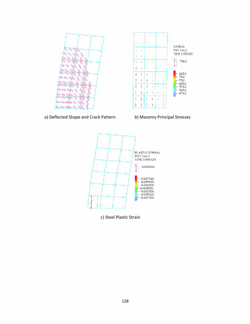
128
a) Deflected Shape and Crack Pattern b) Masonry Principal Stresses
c) Steel Plastic Strain

129
e) Comparison between FE and experimental results
f) Comparison between FE Discretized and Smeared Models
Figure A2.12 Wall 7 (Spacing Mesh) Results
-30
-20
-10
0
10
20
30
-3 -2 -1 0 1 2 3
Load
(K
ips)
Disp. (in)
Peaks
Numerical
Numerical (M)
0
5
10
15
20
25
0 0.5 1 1.5 2 2.5
Load
(K
ips)
Disp. (in)
Discretized
Smeared
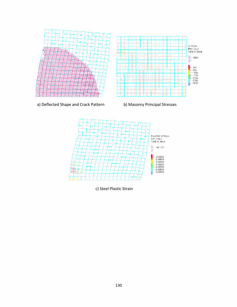
130
a) Deflected Shape and Crack Pattern b) Masonry Principal Stresses
c) Steel Plastic Strain

131
e) Comparison between FE and experimental results
f) Comparison between FE Discretized and Smeared Models
Figure A2.22 Wall 8 (1/4 Spacing Mesh) Results
-80
-60
-40
-20
0
20
40
60
80
-1.5 -1 -0.5 0 0.5 1 1.5
Load
(K
ips)
Disp. (in)
Peaks
Numerical
Numerical (M)
0
10
20
30
40
50
60
70
0 0.1 0.2 0.3 0.4
Load
(K
ips)
Disp. (in)
Discretized
Smeared

132
a) Deflected Shape and Crack Pattern b) Masonry Principal Stresses
c) Steel Plastic Strain

133
e) Comparison between FE and experimental results
f) Comparison between FE Discretized and Smeared Models
Figure A2.23 Wall 8 (1/2 Spacing Mesh) Results
-100
-80
-60
-40
-20
0
20
40
60
80
100
-2 -1 0 1 2
Load
(K
ips)
Disp. (in)
Peaks
Numerical
Numerical (M)
0
10
20
30
40
50
60
70
80
90
0 0.5 1 1.5 2
Discretized
Smeared

134
a) Deflected Shape and Crack Pattern b) Masonry Principal Stresses
c) Steel Plastic Strain

135
e) Comparison between FE and experimental results
f) Comparison between FE Discretized and Smeared Models
Figure A2.24 Wall 8 (Spacing Mesh) Results
-100
-80
-60
-40
-20
0
20
40
60
80
100
-2 -1 0 1 2
Load
(K
ips)
Disp. (in)
Peaks
Numerical
Numerical (M)
0
10
20
30
40
50
60
70
80
90
100
0 0.5 1 1.5 2
Discretized
Smeared