The Design and Regulation of High

Frequency Traders

Professor Daniel Ladley, University of Leicester Working Paper No. 19 02 March 2019

The Design and Regulation of High Frequency Traders

Daniel Ladley∗

University of Leicester School of Business

University of Leicester

LE17RH

UK

March 29, 2019

Abstract

Central to the ability of a high frequency trader to make money is speed. In order to be first

to trading opportunities firms invest in the fastest hardware and the shortest connections

between their machines and the markets. This, however, is not enough, algorithms must be

short, no more than a few lines of code. As a result there is a trade-off in the design of optimal

HFT strategies: being the fastest necessitates being less sophisticated. To understand the

effect of this tension a computational model is presented that captures latency, both of code

execution and information transmission. Trading algorithms are modelled through genetic

programmes with longer programmes allowing more sophisticated decisions at the cost of

slower execution times. It is shown that depending on the market composition short fast

strategies and slower more sophisticated strategies may both be viable and exploit different

trading opportunities. The relative profits of these different approaches vary, however, slow

traders benefit from their presence. A suite of regulations are tested to manage the risks

associated with high frequency trading, the majority are found to be ineffective, however,

constraining the ratio of orders to trades may be promising.

Keywords: Finance, Genetic Programming, High Frequency Trading, Strategy Design, Reg-

ulation

∗E-mail: d.ladley@le.ac.uk, Telephone: +44 (0)116 252 5285. I thank the British Academy and LeverhulmeTrust for their support through the Small Grant scheme. In addition I thank seminar participants at Computingin Economics and Finance, 2017, International Finance and Banking Association, 2017, King’s College Londonand the University of Leicester.

1 Introduction

The phrase ‘time is money’ neatly captures the business model of high frequency trading (HFT).

These traders make money by being the first, whether that’s the first to trade against incoming

orders or the first to revise stale quotes in the event of changing market conditions. Slower

algorithms miss out on the best opportunities and bare more risk. As a result there is an arms

race amongst HFT firms to create algorithms that can identify mispricings and execute new

orders in the fastest time. The time to execute an order depends on several factors: the time

taken for signals to travel between the exchange and the HFT computers, the computer hardware

and the algorithms that run on them. HFT firms pay to minimise the first two factors and not be

at a disadvantage to their competitors. Co-locating of their hardware with that of the exchange1

and purchasing the fastest and most up to date computer hardware. The final component, the

algorithms that govern trade, is the source of competitive advantage for HFT firms but also

represents a trade-off. Longer trading algorithms take more computational cycles to execute

and therefore result in slower actions. By reducing the length of an algorithm the HFT firm

makes their order more likely to be first. Shortening algorithms, however, has a consequence -

reducing the number of lines of code reduces the information processing capacity of the algorithm

- reducing the algorithms ability to identify profitable opportunities and avoid losses. This is

a fundamental trade off in the design of HFT algorithms. The shorter the algorithm the more

likely it is to be first to act but the less sophisticated its strategy.

It is this trade-off that will be the basis of the investigation in this paper. A model is

constructed of the behaviour of HFT algorithms subject to a speed/sophistication trade-off.

HFT traders endogenously decide when to trade based on the actions of others and information

arriving at the market. I analyse the problem faced by HFT strategy designers - what is the

optimal strategy when speed may be traded-off against information processing ability. This

issues has not previously been considered in the literature. Whilst multiple papers have looked

at trading speed in the face of technological costs (see for instance Biais et al., 2015 or Delaney,

2018), they have done so in an environment of perfect rationality. Here I make a unique argument

that the cost of speed is not just monetary but also in terms of cognitive (computational)

sophistication, i.e. in order to increase speed perfect rationality has to be sacrificed. The

extent to which traders are willing to do this is not clear. For instance it is not inevitable that

algorithms will be ever simpler and faster. Unsophisticated trading algorithms may leave money

on the table that slower and more sophisticated HFT’s may identify and capture.

In order to investigate this question it is necessary to have a representation of strategies

where computational sophistication is related to time in a realistic manner. The natural choice

for this is to use a computational approach in which high frequency traders are, like real life,

algorithms. Longer algorithms, as measured by the number of lines of code, generally take more

time to execute as the computer processor must step through each in turn.2 The difficulty of

this approach is then specifying the optimal trading algorithm(s). The relationship between

code length, algorithm design and performance is complex and non-tractable. To resolve this

1To facilitate this many exchanges offer space on their own site with guaranteed lengths of wire betweenmachines to create a level playing field amongst.

2There are exceptions here, conditional statement such as if X do Y can disproportionately slow down executionas they limit the processors ability to cache future actions.

2

I numerically optimise the trading algorithms by competing them against each other within

a market. Maintaining those that do well whilst continuously looking for modifications and

improvements that will enhance performance. This approach of optimising programmes (as

opposed to parameters) is referred to as genetic programming - essentially evolving algorithms

to solve a task.3 For our problem this creates an attractive analogy: a market of trading

algorithms competing to make profits based on their speed and sophistication with the most

successful surviving and the losses being replaced. Given sufficient time this process will lead

to the identification of a steady state in which important details of trading algorithms and

market behaviour no longer change. It is this state, rather than the optimisation process which

produces it that I will analyse. Genetic programming has been used to simulate trading strategies

of different sophistication’s before. Yeh (2008) uses a genetic programming model to show that

greater intelligence improves market efficiency. Ladley et al. (2015) use a genetic programming

model to investigate the relationship between skill and market fragmentation and show that

large numbers of unskilled individuals make the market more susceptible to shocks. Whilst

Manahov et al. (2014) shows that varying the length of trading strategies impacts trader and

market performance. Importantly, however, no work has looked at the trade-off between speed

and sophistication.

Using the model I show that despite competition to be fastest and therefore first to arrive

at a trading opportunity not all HFT’s take this approach in equilibrium. Whilst increasing

competition between HFT’s does push the population towards shorter strategies this is not

universal. Some traders adopt longer strategies and are shown to generate greater per order

(and per trade) profits than those adopting the fastest algorithms. These traders identify and

exploit trading opportunities that their faster competitors miss. As such there are multiple

equilibria in the design of HFT trading strategies.

The presence of HFT’s within the market is shown to be generally positive. Increasing

numbers of HFT’s increase market quality through higher liquidity and lower pricing errors.

At the same time they have relatively little effect on the overall profits of slow traders, instead

their profits come through improved prices and reduced waiting costs for trade. The greater

competition coming from higher numbers of HFT’s leads to reducing profits for this group but

no negative effects for slower traders.

The effectiveness of a suite of regulations proposed to manage the impact of high frequency

traders is considered. The majority, including minimum resting times, speed bumps and in-

creased tick sizes are found to have little or no positive effect, often damaging market quality

and increasing the returns of HFT’s at the expense of slower traders. Transaction taxes are

found to be particularly detrimental to both the market and traders. The only regulation which

potentially has a positive effect are constraints on the ratio of trades to orders submitted by the

HFT’s. This regulation increases the profits of slow traders relative to HFT’s but at the expense

of reducing market liquidity.

The remainder of the paper is organised as follows. Section 2 considers previous work looking

independently at trading speed and the effect of cognitive ability on market performance together

3Genetic Programming has been used in papers for various finance problems. Neely et al. (1997) use theapproach to find technical trading rules, Chen and Wang (2015) use it to construct portfolios, whilst Lensberget al. (2015) and Yeh and Yang (2010) amongst others use this approach to simulate markets.

3

with HFT regulation. Section 3 present a model of a market in which traders trade-off speed

and strategic sophistication. Section 4 presents results showing optimal trading strategies and

market quality whilst Section 5 looks at the effectiveness of regulations. Section 6 concludes.

2 Related Literature

The trade-off between speed and computational time has not previously been considered in

relation to trading. There have, however, been pieces of work that have looked at each factor

individually. The link between intelligence and financial success has been studied extensively.

Some of the earliest work looked at the connection between wages and intelligence (see for

instance Moore, 1911). More recently papers have considered the link between cognitive ability

and stock market performance. Grinblatt et al. (2012) for instance shows that higher IQ leads to

better trading performance whilst Coval et al. (2004) shows that even in the absence of superior

information some traders are able to consistently outperform others, in other words they are

skilled.

The reasons for this out performance may be many fold and have been studied experimen-

tally. Burks et al. (2009) showed that more intelligent players can better predict their opponents

actions in two player sequential games whilst Corgnet et al. (2015) find that high intelligence

traders are more likely to identify points at which the asset is under priced or overpriced com-

pared to their low cognitive ability compatriots. Chen et al. (2017) analyses which aspects of

intelligence are responsible for the higher returns of traders and find that this varies depending

on the types of individuals they are competing against. The effect on the market of cognitive

ability has also received some attention. Breaban and Noussair (2015) show experimentally

that higher cognitive ability results in prices being closer to fundamental values, while Noussair

et al. (2016) show that in an experimental setting more intelligent individuals lead to a closer

relationship between the fundamental and market price.

High frequency trading has received a great deal of attention in recent years from both

theoretical and empirical analysis. Papers have considered liquidity (Hendershott et al., 2011),

price discovery (Brogaard et al., 2014) and strategy effects (Hagstromer and Norden, 2013)

amongst other issues.4 Several papers have focused on the effect of increased speed however

the findings are ambiguous. For instance Foucault et al. (2013) examines the cost of being first

in terms of continuous monitoring of markets while Brogaard et al. (2015) exploits a natural

experiments to show that increased speed, as a result of market makers co-locating, benefits the

market by enhancing liquidity. Similarly Riordan and Storkenmaier (2012) show that a decrease

in latency leads to greater price efficiency and increased liquidity. In contrast Foucault et al.

(2017) argue that increased speed leads to greater illiquidity and that while HFT arbitrageurs

may increase price efficiency they also increase picking off risk. Menkveld and Zoican (2017)

show that speeding up high frequency trading does not necessarily improve liquidity and that the

effect will vary based on ratio of news to liquidity traders. There has been particular attention

around the role of HFT’s in flash crashes (see Kirilenko et al., 2017, for a discussion) and systemic

risk e.g. Paulin et al. (2019). The best way to deal with the potentially destabilising effects of

4See Menkveld (2016) for a recent survey.

4

high frequency trading, however, is unclear: Biais et al. (2015) argue that a tax as opposed to

a ban is most beneficial to the market. Budish et al. (2015) in contrast looks at the optimal

market architecture and argues that moving from continuous double auctions to discrete batch

auction reduces the value of very small speed advantages and so encourages competition on price

instead of speed, benefiting market participants.

Leal and Napoletano (2017) use an agent based model to consider flash crashes and the

effect of several regulations. Their model is based around slow traders and HFT’s who use

pre-specified strategies (although slow traders may switch between chartist and fundamentalist

strategies) to submit orders within trading windows of fixed length. They show how circuit

breakers, cancellation fees, minimum resting times and transaction taxes affect the probability

and recovery from flash crashes, notably with all but the first reducing market volatility and flash

crashes but increasing the duration of these events when they occur. The model has similarities

with the approach taken in this paper, however, differs in two key respects. Firstly trading

strategies within this paper are endogenously determined based on the trade-off of speed and

sophistication with an aim of maximising profits. Secondly trade within this paper happens

within an ongoing continuous setting rather than discrete windows. As such the timing and

frequency of trade is endogenous and determined by the traders own strategy and the actions

of other traders, allowing traders to respond multiple times to each other in quick succession.

3 Model

I consider a continuous time model of the trade of a single financial asset. The asset is traded

through an order book which is defined in the standard manner. It consists of a discrete series of

equidistantly spaced prices at which orders may be submitted. The set of prices is Π = {pi}∞i=−∞whilst the distance between adjacent prices is referred to as the tick size and is equal to δp. Each

price has an associated queue of unfilled orders, potentially of size zero, available at that price,

lit. Each order specifies the quantity to be traded with negative values indicating sell orders

and positive values representing buy orders. The set of queues together comprise the order

book L = {lit}∞i=−∞. The best bid is defined as the highest price at which there is an unfilled

buy order (B(L) = max{i|li > 0}) whilst the best ask is the lowest price at which there is an

unfilled sell order (A(L) = min{i|li < 0}). To address cases where no buy orders or sell orders

are present,define l−∞ = 1 and l∞ = −1. An order submitted to the book comprises a price

quantity pair (p, q). If an order is submitted where q > 0 (q < 0) and p ≥ A(L) (p ≤ B(L)) the

order is treated as a market order and a trade occurs at the best ask (bid). If q > 0 (q < 0) and

p < A(L) (p > B(L)) the order is treated as a limit order and added to the back of the queue

lp. As such the order book operates under price and time priority.

The fundamental value of the asset is defined as vt at time t. Innovations to the fundamental

value are exponentially distributed with mean λv. Each innovation consists of the fundamental

value increasing or decreasing by δp with equal probability. The initial value of the fundamental

value v0 is constrained to lie on the price grid Π and therefore at all points in time vt ∈ Π.

The market is populated by two groups of traders: High frequency traders who have no

intrinsic value for holding the asset and slow traders who buy or sell the asset for exogenous

reasons such as liquidity, hedging or speculation.

5

3.1 Slow Traders

Slow traders are risk neutral and attempt to maximise their profits from trade. Each slow trader

has a private valuation αi relative to the fundamental value. A slow trader attempts to maximise

e−ρT qi(vt + αi − pi) (1)

where pi is the trade price and qi is the traded quantity. ρ is a discount factor and T is the

length of time from the traders original entry to the market to the time of trade. The discount

factor represents the cost of waiting to transact either from lost opportunities of mis-hedging

costs. It does not represent interest on capital as over these timescales this would be negligible.

Slow traders arrive at the market according to an exogenous process. The times between

new trader arrivals are exponentially distributed with mean λa. On arrival a trader submits an

order to buy or sell a single unit of the asset. The price and direction are selected to maximise

the traders profits as determined by the traders strategy (described below).

Slow traders may re-enter the market and revise unexecuted orders any number of times.

The trader reenters at a random point in the future drawn from an exponential distribution with

mean λr. Traders may therefore not instantly revise orders and are exposed to picking off risk.

The trader may only re-enter if their original order has not executed. When a trader re-enters

the market they have the option of keeping their existing order or cancelling it and submitting

a new order. A trader may continue to re-enter the market and revise their order until it has

executed and they leave the market forever.

3.2 High Frequency Traders

HFT’s trade based on the order flow, buying the asset when it is under-priced and selling it

when it is overpriced. Nh HFT’s are present in the market at the start and persist throughout

its lifetime executing multiple trades. Initially these traders do not have an order in the market.

HFT’s act in one of two circumstances. HFT’s may act in response to new orders from other

traders as they arrive at the market. If an order arrives at the market at time T0, an HFT

responds at time T0 + Di where Di is the time taken for information about the arrival of an

order to be transmitted to market participant i through the connective technology. As such

the actions of slow traders and other HFT’s may stimulate an HFT trader to act which may

in turn stimulate other HFT’s to act. As such HFT’s as a group may generate cycles of high

frequency order revisions. In addition to this, like slow traders HFT’s periodically re-enter the

market and revise unexecuted orders. The times of these reentries are randomly determined

with intervals being exponentially distributed with mean λr and each traders random entry

times being independent of all others. A new reentry time is drawn after each occasion a HFT

acts. Note that λr is much larger than Di, therefore this random reentry plays no role in

concentrated periods of HFT interaction, rather it provides the opportunity for HFT’s to act

during quiet periods when their is little going on in the market.

HFT traders may submit, revise orders and trade any number of times. When an order

6

executes with price pi and quantity qi the HFT receives profit:

e−ρT qi(vt − pi) (2)

where T is measured from the traders last trade time. Importantly unlike slow traders, fast

traders have no inherent value in holding the asset. Given HFT’s are always in the market they

may be interpreted as maximising their rate of profits - i.e. the speed with which they make

money.

3.3 Order Submission

Upon arriving at, or reentering, the market a trader of either type submits an order which

comprises a price quantity pair a = (p, q). p is the price such that p ∈ Π whilst q is the quantity

such that q ∈ −1, 0, 1. A quantity of zero represents the choice to not submit an order, in which

case the value of p is irrelevant. Additionally a trader with an existing unexecuted order in the

market may choose to keep that order and maintain time priority.

The order submission decision is determined by the trader’s strategy. Trader strategies take

information about the state of the market as input and provide as output a price quantity pair as

described above. The mapping between these, however, is non trivial due to the complex market

architecture and interaction with other strategies. I therefore use a computational optimisation

process to identify the optimal trading strategies for both groups of traders.

Traders strategies are specified through algorithms - list of instructions detailing the pro-

cessing of market information to arrive at an action. These algorithms are identified through

Genetic Programming - an evolutionary approach to optimisation. It works through selecting

successful ‘fit’ strategies, in this case those that make the most money, and reproducing them

in the population of candidate solutions. The reproduced strategies are subject to mutation

- small perturbation’s to the algorithms instructions. Over time the combination of selection,

reproduction and mutation result in optimisation of the population of candidate strategies.

In this paper I use Cartesian Genetic Programming.5 Whilst there are many versions of

genetic programming this approach was chosen for its speed, constrained memory usage, and

interpretability. In this specification of genetic programming the programme is represented in

a graph format. Each strategy has NI inputs which take numerical values describing the state

of the world. The programme comprises NN nodes indexed 1, ...NN . Each node is a control

statement or mathematical function6 which takes a number of inputs and provides a single

output. For arithmetic operators this is the result of applying the operator on the two inputs.

Control statement are of the form ‘if then else’ which compares the first two inputs and returns

either the third or fourth input depending on the comparison.7 The inputs to node k are either

the outputs of other nodes with index < k or one of the programme inputs. The outputs of the

programme are taken from the values of the final two nodes.

The programme executes by evaluating the nodes from 1 to NN in turn. Not every node

of the programme effects the result calculated. Only those nodes connected to the output (and

5See Turner and Miller, 2014 for details6Drawn from ‘+’,‘-’,‘×’,‘÷,‘abs’,‘max’,‘min’,‘if...then’.7Drawn from ‘>’,‘=’

7

those recursively connected to those) will have an effect. Nodes not within this set play no

role. I term the length of the programme to be the number of nodes which contribute to the

output. As such I assume that those nodes that do not contribute are not executed. The initial

population of programmes are randomly generated. The operators and node inputs are selected

at random from the available sets with equal probability.

A strategy’s fitness is measured as its average payoff. For both types of traders this is the

total profit obtained by traders using a strategy divided by the number of times traders using

the strategy have executed orders. Reproduction occurs through genetic tournaments. Every tt

time steps two strategies are selected at random. The strategy with lowest fitness is replaced

by a copy of the strategy with higher fitness. The copied strategy is mutated. Each node

and connection in the strategy undergoes a mutation with probability pm. A mutation of a

node leads to the function associated with that node being replaced by a different randomly

chosen function with uniform probability. A mutation to a connection or output results in a

different node or programme input being attached at random across all possibilities with equal

probability. The mutated strategy has the total profit and number of orders submitted using

the strategy reset to zero.

When a slow trader arrives at the market they are randomly allocated a strategy from

the population of candidate slow trader strategies. They keep this strategy until their trade

has executed and they leave the market. Similarly an HFT trader is randomly allocated a

strategy from the population of candidate HFT strategies when they enter the market. They

maintain this strategy until they have traded, at which point they are randomly allocated a new

strategy. Importantly, fitness is associated with strategies rather than traders. There are at any

time a fixed number of HFT’s in the market, defining the level of HFT activity, however, the

strategies of these HFT’s will vary over time. The random selection of a strategy ensures that all

candidate strategies are evaluated within the market for their potential to make profits. Separate

populations are maintained for both slow and HFT traders to reflect the differing tasks they are

faced with. Each population is broken down into groups - a partitioning of the the population

of strategies into NG equally sized segments. When strategies are chosen for reproduction they

are selected from the same group. This prevents the spread of one successful strategy across the

whole population and supports the existence of multiple solutions if viable.

3.4 Time

When a trader arrives at the market at time t to submit an order they observe the state of the

market at time t−Di where Di is the amount of time it takes for information about the market

to travel via the connective technology to the trader.

Di =

tH , if i = H

tS , if i = S(3)

where tH < tS i.e. HFT’s are closer (co-located) to the market than slow traders and receive

information more quickly. Fast traders react to an order submitted to the market at time tH

after the order has arrived, i.e. time for the information about the order to reach the trader.

When a trader chooses to submit an order, either on entry to the market or in response to

8

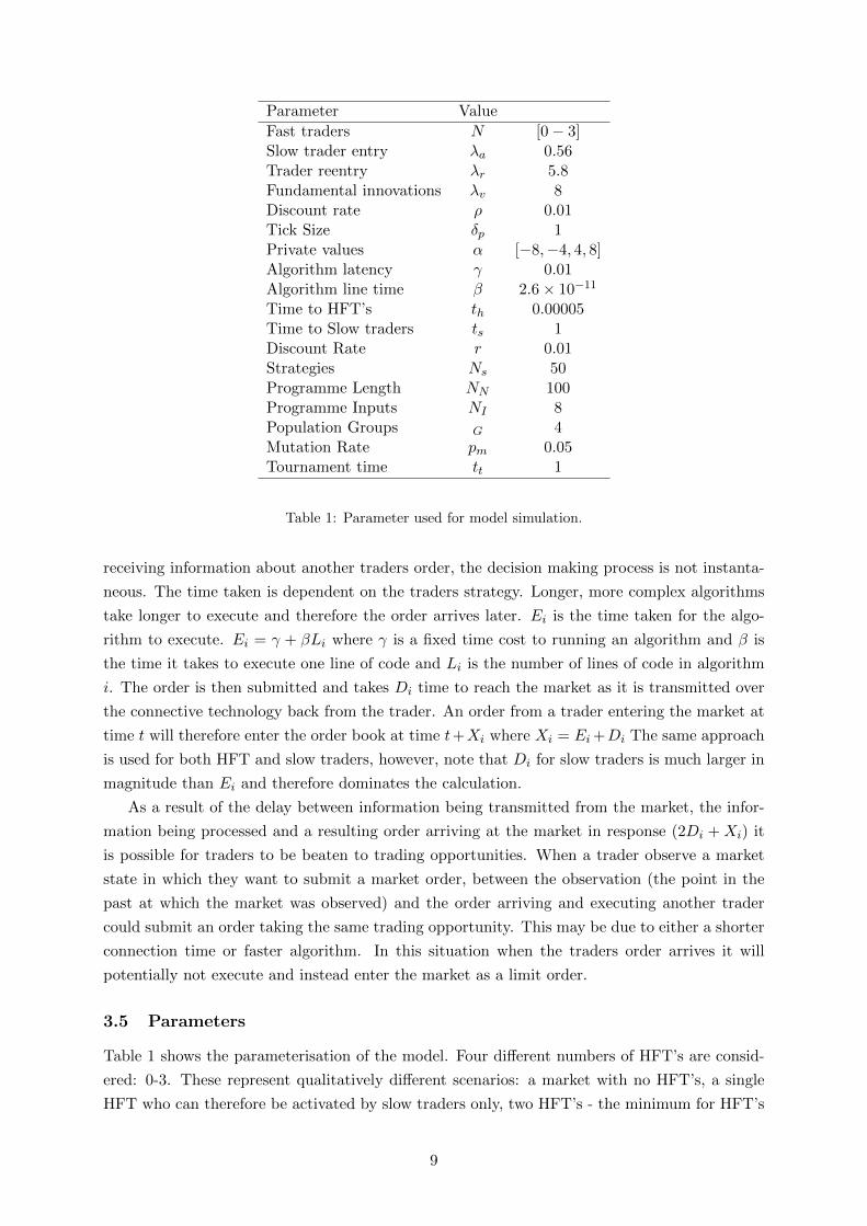
Parameter Value

Fast traders N [0− 3]Slow trader entry λa 0.56Trader reentry λr 5.8Fundamental innovations λv 8Discount rate ρ 0.01Tick Size δp 1Private values α [−8,−4, 4, 8]Algorithm latency γ 0.01Algorithm line time β 2.6× 10−11

Time to HFT’s th 0.00005Time to Slow traders ts 1Discount Rate r 0.01Strategies Ns 50Programme Length NN 100Programme Inputs NI 8Population Groups G 4Mutation Rate pm 0.05Tournament time tt 1

Table 1: Parameter used for model simulation.

receiving information about another traders order, the decision making process is not instanta-

neous. The time taken is dependent on the traders strategy. Longer, more complex algorithms

take longer to execute and therefore the order arrives later. Ei is the time taken for the algo-

rithm to execute. Ei = γ + βLi where γ is a fixed time cost to running an algorithm and β is

the time it takes to execute one line of code and Li is the number of lines of code in algorithm

i. The order is then submitted and takes Di time to reach the market as it is transmitted over

the connective technology back from the trader. An order from a trader entering the market at

time t will therefore enter the order book at time t+Xi where Xi = Ei+Di The same approach

is used for both HFT and slow traders, however, note that Di for slow traders is much larger in

magnitude than Ei and therefore dominates the calculation.

As a result of the delay between information being transmitted from the market, the infor-

mation being processed and a resulting order arriving at the market in response (2Di + Xi) it

is possible for traders to be beaten to trading opportunities. When a trader observe a market

state in which they want to submit a market order, between the observation (the point in the

past at which the market was observed) and the order arriving and executing another trader

could submit an order taking the same trading opportunity. This may be due to either a shorter

connection time or faster algorithm. In this situation when the traders order arrives it will

potentially not execute and instead enter the market as a limit order.

3.5 Parameters

Table 1 shows the parameterisation of the model. Four different numbers of HFT’s are consid-

ered: 0-3. These represent qualitatively different scenarios: a market with no HFT’s, a single

HFT who can therefore be activated by slow traders only, two HFT’s - the minimum for HFT’s

9

to activate each other and three HFT’s in which there is a greater possibility for cycles of

activation.

The choice of λa and λr are inline with previous simulation studies of high frequency order

book markets such as Chiarella and Ladley (2016) and Bernales (2016). In both cases these

papers use empirical data to estimate arrival and reentry times of traders. The fundamental

innovation rate λv is inline with estimates used by Goettler et al. (2009). As discussed above

the discount rate, ρ, does not represent the risk free rate in this model rather it represents the

cost of not trading and includes factors such as attention costs, missed opportunities through

not executing and mis-hedging. The model was tested with other small positive values and

qualitatively similar results were obtained.

Slow trader private values, αi, are drawn randomly and independently with the following

support [8, 4,−4,−8]. 8 and -8 each have probability 0.2 whilst 4 and -4 have probability 0.3.

The relative sizes of these probabilities are based on the distributions estimated by Hollifield

et al. (2006) for private valuations of traders in the Vancouver stock exchange. One important

difference between this work and theirs is that I do not allocate any slow traders a private

valuation of zero. This is because the high frequency traders implicitly have this valuation and

therefore provide this component of the private value distribution.

The trading time parameters are based on empirical observation. Note that these values

vary in real life between markets and technologies, I therefore take values consistent with the

majority of the literature. The algorithm latency is take from Riordan and Storkenmaier (2012)

and is inline with figures quoted by Menkveld and Zoican (2017). The travel time to HFT’s is

based on the Nasdaq estimate of round trip latency.8 The algorithmic line time is estimated

from the specification of an AMD Ryzen 7 processor. Note, however, that the exact figure used

here is unimportant - it is sufficient that is it much smaller than the latency, γ.

The genetic programmes have eight inputs - the current best bid and best ask prices along

with the quantities available at both of these quotes. They also take the trader’s private valu-

ation, which is zero for HFT’s. In addition if the trader has an order in the market they know

the price, quantity and priority of that order in the execution queue. All prices in the above

are measured relative to the fundamental price. This has the advantage of simplifying the trad-

ing decision by removing the level effect. As such the fundamental value is known by traders

implicitly rather than as a explicit parameter.

Simulations are run for 500000 periods each of 5000 time steps. At the end of each period

the fitness of all strategies is reset to zero. This helps to prevent the optimisation getting stuck

in local equilibria. Each simulation is repeated 1000 times with different random seeds in order

to control for randomness.

4 Results

The results of the model are presented in two parts. The first focuses on the strategies and

profitability of HFT’s in the market before considering their effect on market quality. The

second group of results examines the effect of a suite of regulations on market quality and the

8See http://www.nasdaqtrader.com/Trader.aspx?id=COLO

10

Slow Traders - 4 Slow Traders - 8Number Waiting Waiting HFT Slow HFTHFT’s Cost Profit Cost Profit Profit Length Length

0 -0.56 3.47 -1.14 6.70 44.79(0.23) (0.22) (0.43) (0.38) (12.04)

1 -0.43 3.46 -0.88 6.83 1.01 44.43 36.68(0.20) (0.21) (0.37) (0.40) (1.06) (11.90) (12.41)

2 -0.40 3.47 -0.81 6.89 0.81 44.55 30.05(0.19) (0.21) (0.36) (0.40) (0.74) (12.43) (11.40)

3 -0.38 3.44 -0.78 6.86 0.77 44.21 28.49(0.20) (0.25) (0.37) (0.48) (0.85) (11.69) (11.60)

Table 2: Gains from trade. The table shows the average profit per trade for the three groups of traders:HFT’s, Slow (valuation 4/-4) and Slow (valuation 8/-8). In addition it shows the waiting cost for eachtrade, defined as |e−ρTα| where T is the time between entry and trade, i.e. the reduction in potentialprofits from the private value as a result of time passing between the trader entering the market andexecuting the trade. This is always zero for HFT’s due to them implicitly having a private valuation ofzero. In addition for the two categories of trader, Slow and HFT, the table also shows the average lengthof the algorithm. All results are average over 1000 repetitions for each quantity of HFT’s. Standarddeviations are show in parenthesis.

behaviour of traders.

4.1 Trading Strategies

Previous work has ignored the effect of the trade off between speed and sophistication on the

design of HFT trading strategies and their resulting success. Table 2 shows the average profits

of slow and high frequency traders within the market. The presence of HFT’s has very little

effect on the profits of slow traders. For slow traders with a valuation of |4| the average profit

with or without HFT’s is not statistically different. Whilst for those with a valuation of |8|there is a small increase in the presence of HFT’s but no statistical difference for different

numbers of HFT’s. In both cases the money lost due to waiting decreases, indicating that

HFT’s are providing a benefit through faster execution. At the same time, however, the smaller

improvement in overall profits indicates that HFT’s are capturing some of the gains from trade

as a result of faster execution and slow traders are trading at worse prices. The result of this is

that HFT’s obtain positive profits per order. As the number of HFT’s increases the per trade

profits decrease. Competition to be first means that HFT’s have to take less favourable prices,

reducing gains. The impact of HFT’s on slow traders is therefore positive but mixed - they

provide immediacy at the cost of less favourable trading prices.

In addition to reducing HFT profits Table 2 shows that the competition between HFT’s also

reduces the average length of these algorithms. Increasing competition to be first to a trading

opportunity results in algorithms becoming shorter and faster in order to minimise execution

time. This is inline with our initial discussion. In contrast the length of slow trader algorithms

is not statistically different across different specifications. The impact of the shortening in

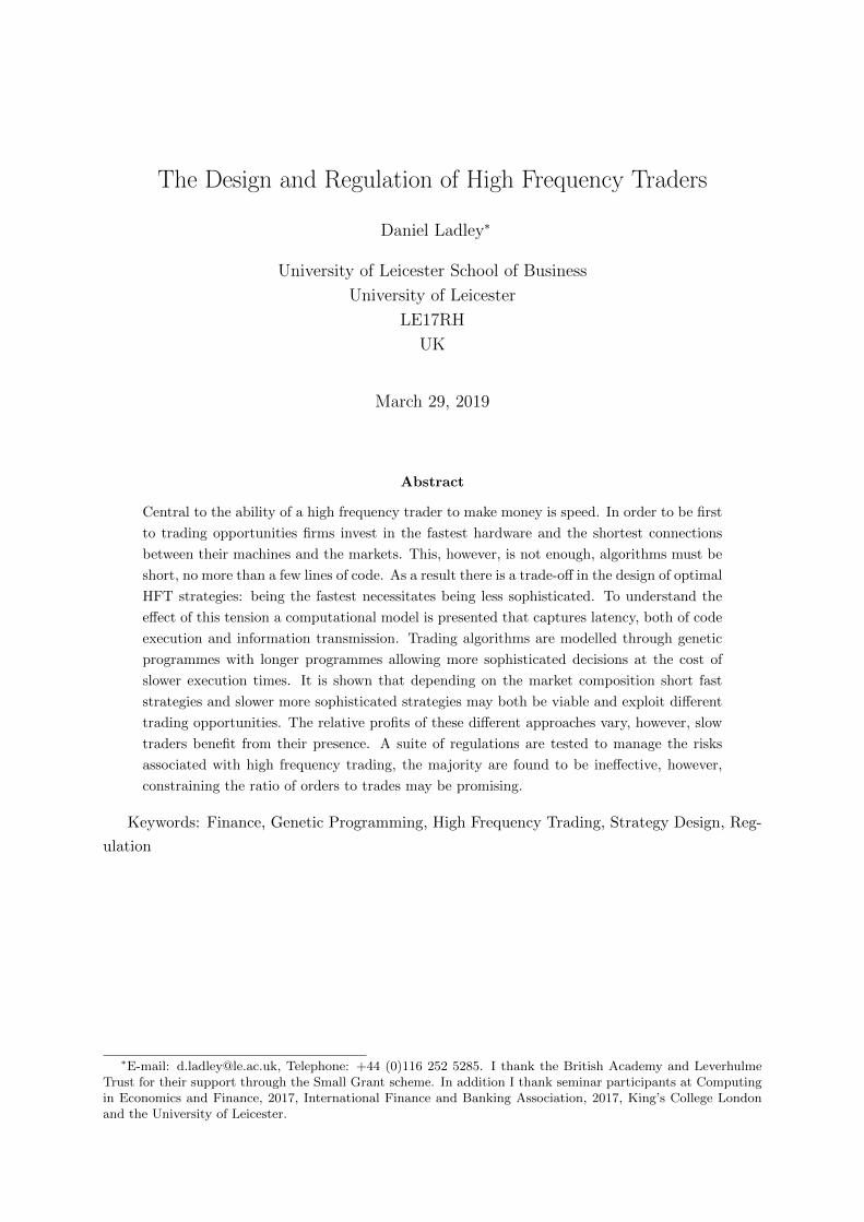
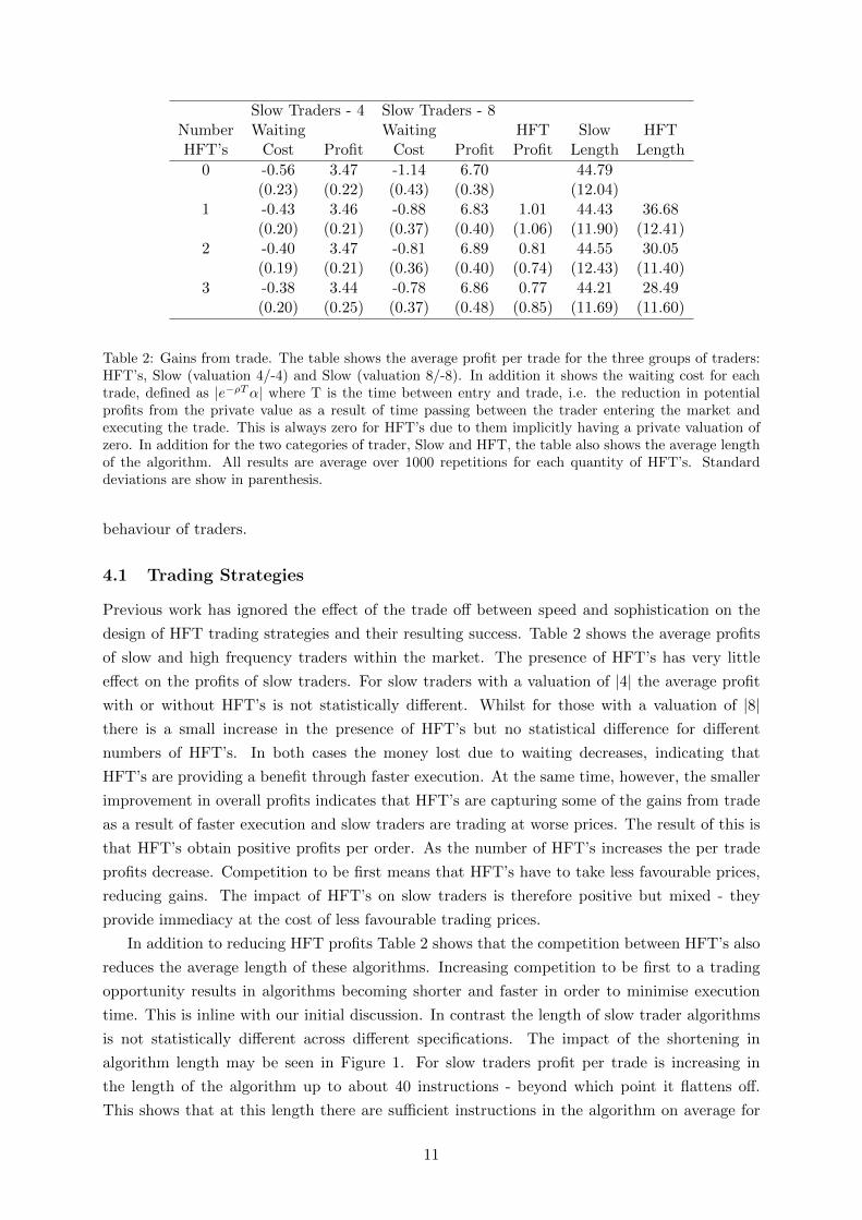
algorithm length may be seen in Figure 1. For slow traders profit per trade is increasing in

the length of the algorithm up to about 40 instructions - beyond which point it flattens off.

This shows that at this length there are sufficient instructions in the algorithm on average for

11

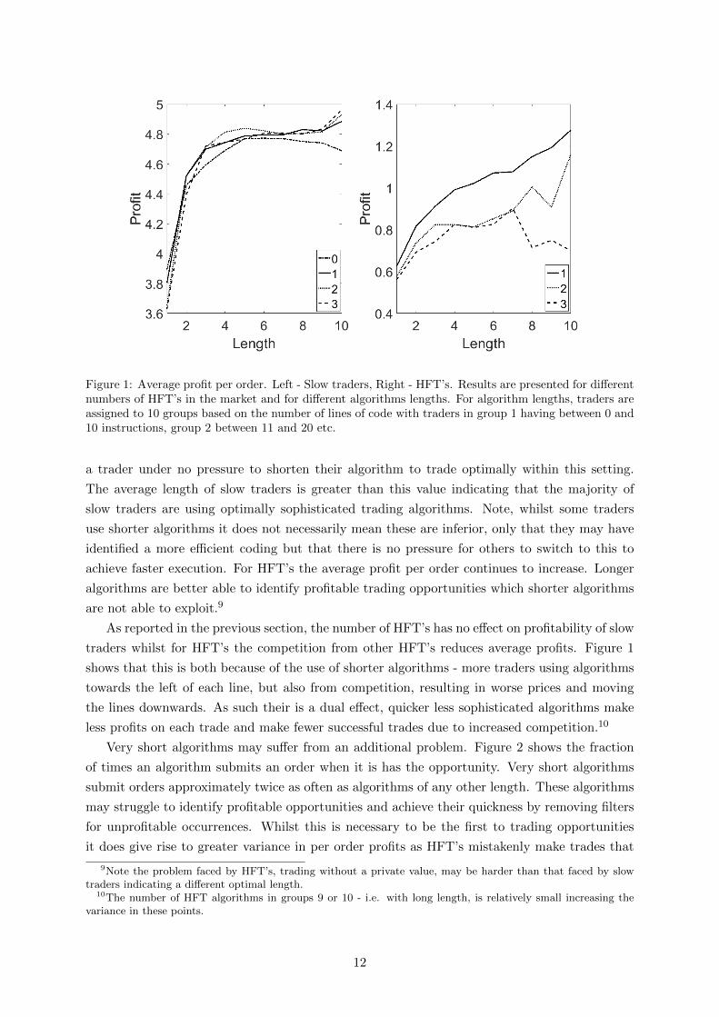
Figure 1: Average profit per order. Left - Slow traders, Right - HFT’s. Results are presented for differentnumbers of HFT’s in the market and for different algorithms lengths. For algorithm lengths, traders areassigned to 10 groups based on the number of lines of code with traders in group 1 having between 0 and10 instructions, group 2 between 11 and 20 etc.

a trader under no pressure to shorten their algorithm to trade optimally within this setting.

The average length of slow traders is greater than this value indicating that the majority of

slow traders are using optimally sophisticated trading algorithms. Note, whilst some traders

use shorter algorithms it does not necessarily mean these are inferior, only that they may have

identified a more efficient coding but that there is no pressure for others to switch to this to

achieve faster execution. For HFT’s the average profit per order continues to increase. Longer

algorithms are better able to identify profitable trading opportunities which shorter algorithms

are not able to exploit.9

As reported in the previous section, the number of HFT’s has no effect on profitability of slow

traders whilst for HFT’s the competition from other HFT’s reduces average profits. Figure 1

shows that this is both because of the use of shorter algorithms - more traders using algorithms

towards the left of each line, but also from competition, resulting in worse prices and moving

the lines downwards. As such their is a dual effect, quicker less sophisticated algorithms make

less profits on each trade and make fewer successful trades due to increased competition.10

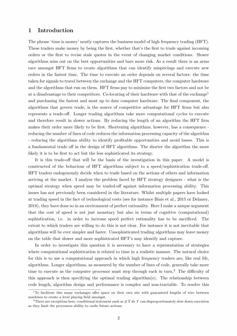
Very short algorithms may suffer from an additional problem. Figure 2 shows the fraction

of times an algorithm submits an order when it is has the opportunity. Very short algorithms

submit orders approximately twice as often as algorithms of any other length. These algorithms

may struggle to identify profitable opportunities and achieve their quickness by removing filters

for unprofitable occurrences. Whilst this is necessary to be the first to trading opportunities

it does give rise to greater variance in per order profits as HFT’s mistakenly make trades that

9Note the problem faced by HFT’s, trading without a private value, may be harder than that faced by slowtraders indicating a different optimal length.

10The number of HFT algorithms in groups 9 or 10 - i.e. with long length, is relatively small increasing thevariance in these points.

12

Figure 2: Submission ratio - the number of orders submitted by the trader divided by the number ofchances they have to submit orders. Left - Slow traders, Right - HFT’s. Results are presented for differentnumbers of HFT’s in the market and for different algorithms lengths. For algorithm lengths, traders areassigned to 10 groups based on the number of lines of code with traders in group 1 having between 0 and10 instructions, group 2 between 11 and 20 etc.

result in low profits in some cases. The positive effect of HFT’s on slow traders may also be

seen in Figure 2 as greater numbers of HFT’s increase the fraction of slow trader orders that

execute, therefore reducing weighting costs.

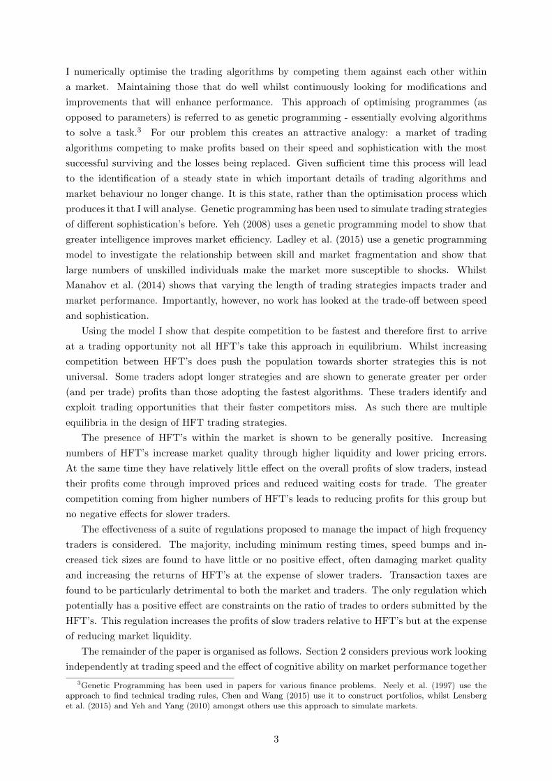
Figure 3: Fraction of orders submitted by traders. Left - Slow traders, Right - HFT’s. Results arepresented for different numbers of HFT’s in the market and for different algorithms lengths. Fractionof orders is the number of orders submitted by traders of that type and length divided by the totalnumber submitted by that type across all strategy lengths. For algorithm lengths, traders are assignedto 10 groups based on the number of lines of code with traders in group 1 having between 0 and 10instructions, group 2 between 11 and 20 etc.

13

Number Best Ask Total Ask PricingHFT’s Spread Quantity Quantity Volatility Error

0 2.62 10.0 61.6 0.85 2.25(0.51) (5.4) (55.8) (0.36) (0.55)

1 2.34 7.7 42.0 0.90 1.79(0.44) (4.5) (47.8) (0.28) (0.57)

2 2.15 7.0 36.1 0.91 1.60(0.48) (4.0) (40.0) (0.28) (0.58)

3 2.02 6.9 38.3 0.89 1.52(0.52) (4.5) (45.8) (0.24) (0.66)

Table 3: Market quality. All results are average over 1000 repetitions for each quantity of high frequencytraders. All distance measures are in ticks whilst quantity measures are in units. The quantities atthe best bid and in the buy book are similar to those at the best ask and in the ask book. Volatility ismeasured in ticks over 10 minute in model periods. Pricing error is the average absolute distance betweenthe mid point of the spread and the fundamental value. Standard deviations are in parenthesis.

Figure 3 shows the number of orders submitted by each type of trader conditional on al-

gorithm length. For slow traders the curves overlap and show that most traders have a very

similar algorithm length. There is no competition over algorithm speed and therefore no incen-

tive to shorten algorithms below the approximately 40 instructions needed to trade effectively.

For HFT’s the number of orders submitted by different algorithms differs markedly for different

market configurations. When there is only a single HFT the distribution is similar in shape to

that of slow traders - i.e. indicating no incentive to shorten the length of code. The introduction

of a second HFT, however, changes this markedly. Instead of peaking around 40 instructions

algorithms with 0-10 instructions are seen to submit the most orders with a monotonic decrease

in orders submitted as length increases. A further HFT makes this pattern more pronounced

with an even greater share of orders being submitted by very short algorithms. This clearly

demonstrates competition on algorithmic speed. The introduction of a second competitor al-

gorithm pushes traders to reduce the length of their code with further traders increasing this

pressure. It is important to highlight that the differences in execution time are very small as

the line execution time is 2.6 × 10−11. Whilst the effect on the absolute time for execution is

small, the relative effect - being shortest and therefore first to the trading opportunity, is crucial

to success. The strategy of these short HFT’s is clear, taken together with those results in

Figure 1, these traders make large numbers of trades with relatively small profits. In contrast

those HFT’s who use longer algorithms submit fewer orders but make greater profits per trade.

As such their is a continuum of viable HFT strategies ranging from quick and unsophisticated

to slower and intelligent all of which make profits. The distribution of traders types within the

market effects the relative mix of strategies in equilibrium.

4.2 Market Quality

The effect of HFT’s on the functioning of markets has received much interest, in particular

the role they play on liquidity, price efficiency and stability are all areas of discussion. Table 3

presents results showing the effect of different levels of high frequency trading on market quality.

High frequency traders are shown to have an ambiguous effect on liquidity - they narrow the

14

spread but also reduce the quantities available both at the best quotes and throughout the

book as a whole. This agrees with the empirical observations of Korajczyk and Murphy (2018)

who find that a reduction in HFT’s widens spreads and reduces price impact. HFT’s are able

to respond to information more quickly than slow traders, as a result they are able to narrow

the quotes without being subject to the same degree of picking off risk and at the same time

are able to quickly match any orders from other traders that become stale. The presence of

multiple HFT’s also creates competition forcing HFT’s and other traders to shave their prices

and narrow the spread in order to trade. This ability to respond quickly to information and

maintain a narrow spread results in lower average pricing error - the market better tracks the

fundamental. Importantly, whilst the average error goes down the variance in the pricing error

goes up. This is because groups of HFT’s can respond to each others order’s repeatedly and so

generate quote churn which is not associated with information or trading needs.

This effect is also evidenced in the volatility as measured by changes in the mid price. The

presence of HFT’s leads to an increase in volatility from the adjustment of quotes and picking

off of orders by HFT’s responding quickly to the changing market. Whilst HFT’s increase

volatility, the number of HFT’s has no statistically significant effect. The presence of only one

HFT is sufficient to observe this effect. One HFT is able to respond to every action within the

market whilst multiple HFT’s respond to each other. Volatility, however, is only measured at set

intervals these very fast HFT interactions have little effect on the market dynamics as measured

by volatility.

5 Regulation

There has been much debate about the regulation of financial markets in the presence of HFT’s.

In particular HFT’s have been accused of damaging market quality and inhibiting trading op-

portunities for other traders. As a result, a suite of regulations have been proposed to limit the

dangers of HFT’s and their participation in the market or to drive them from the market all

together. In this section I consider six possibilities.

5.1 Specification

Each regulation comprises a modification of the above model above. I consider each regulation

separately versus the case of a market comprising three HFT’s and no regulations.

5.1.1 Make/Take Fee

Make take fees have been common within markets for a number of years and serve as an im-

portant benchmark for understanding the role of market design and regulation on HFT’s. They

have been shown to effect the behaviour of HFT’s and therefore the market liquidity (Foucault

et al., 2013). Make take fees work by imposing a costs ζ on the submitter of a market order

(whether that is an order to buy or sell) and at the same time by paying a limit order supplier

who’s order successfully executes a fee of ζ (again regardless of whether they are a buyer or

seller). The market order fee is often larger than the limit order supplier fee in order to provide

a small profit to the exchange, however, in this model we abstract from this assumption.

15

5.1.2 Tick Size

High frequency traders often make money through offering small improvements on the best

quotes. In order to limit their ability to do this it has been proposed to increase the tick size.

This effectively increases the cost to improving on the best quotes. Within the base model we

take a tick size δp = 1. Under this regulation the tick size in increased. This means that all

orders may only be placed on a price grid in which prices are separated by larger increments.

Note in order that the fundamental value also remains on the ticks the size of fundamental

changes is increased to match the new tick size whilst rate of innovations is reduced such that

the fundamental volatility remains the same as the base case.

5.1.3 Speed Bump

One proposed method to reduce the speed advantage of HFT’s is to delay the arrival time of

their orders. This approach is frequently referred to as a speed bump. The effect of this is to

limit the benefits of being fast, as despite reacting to information quickly their is delay in acting.

Without the regulation an order submitted at time t reaches the order book at time t+Di where

Di is a fixed time dependent on the class of traders. With this regulation the order arrival time

is: t + Di + ψ where ψ is the time taken for the arriving order to cross the speed bump. Note

the speed bump does not effect the speed of dissemination of information going in the opposite

direction.

5.1.4 Minimum Resting Time

An alternative way to slow down and limit the advantage of HFT’s is to limit how quickly they

can change the orders submitted to the book. Rather than delaying orders arriving at the book

it has been proposed to require orders submitted by traders to spend a minimum amount of time

resting in the book before they can be changed or cancelled. I refer to this minimum resting

time as ω. Within the model an order cannot be changed until ω seconds have passed since the

order reached the book. In practical terms a high frequency trader i, submitting an order at

time t, will next become active and look at their order at time t+ω−Di−Ei. This is the time

such that the trader will be able to change their order at the first available time point after the

order becomes available for modification.

5.1.5 Order Ratio

High frequency traders often rapidly change their orders to respond to other HFT’s and changes

in the market. In order to limit this advantage of HFT’s and make the market more transparent

several exchanges limit the ratio of orders an HFT can submit relative to the number of trades

(Menkveld, 2013, see for instance Chi-X as discussed by). Within this model this calculation is

performed for each trading algorithm. At its creation, either at the start of the simulation or

through a tournament, algorithm i’s count of trades, ξMi , and orders, ξLi , are set to 0. Every

order a trader submits, whether a market or limit order, is added to the respective counts. A

trader may only submit a limit order if the ratioξMiξLi

> Ξ, otherwise they must submit a market

order, guaranteeing a trade, or take no action.

16

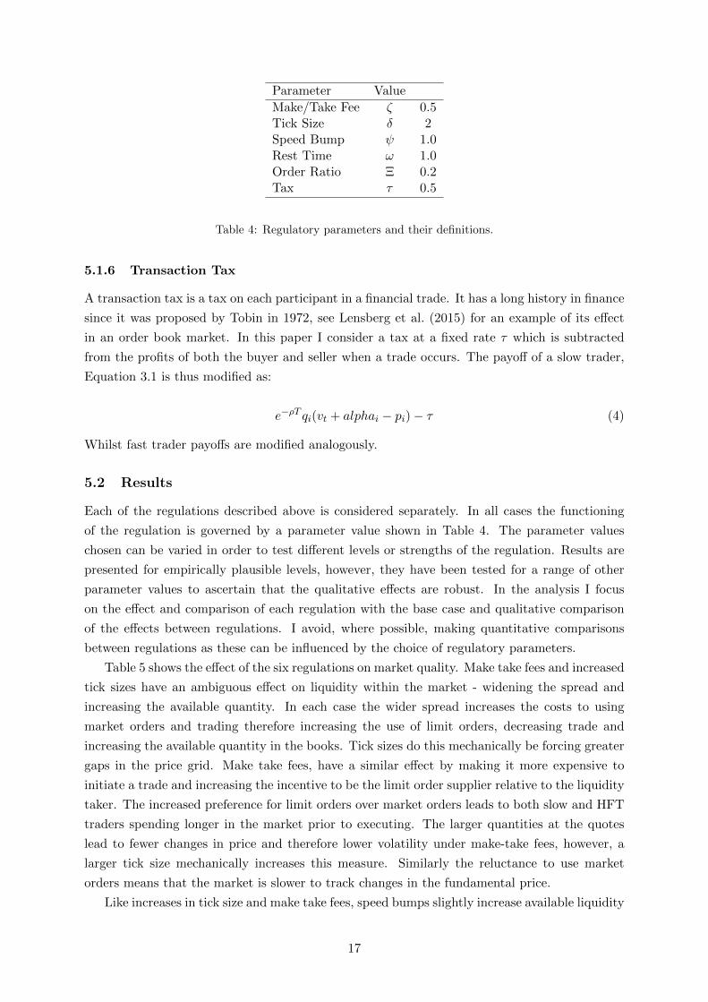
Parameter Value

Make/Take Fee ζ 0.5Tick Size δ 2Speed Bump ψ 1.0Rest Time ω 1.0Order Ratio Ξ 0.2Tax τ 0.5

Table 4: Regulatory parameters and their definitions.

5.1.6 Transaction Tax

A transaction tax is a tax on each participant in a financial trade. It has a long history in finance

since it was proposed by Tobin in 1972, see Lensberg et al. (2015) for an example of its effect

in an order book market. In this paper I consider a tax at a fixed rate τ which is subtracted

from the profits of both the buyer and seller when a trade occurs. The payoff of a slow trader,

Equation 3.1 is thus modified as:

e−ρT qi(vt + alphai − pi)− τ (4)

Whilst fast trader payoffs are modified analogously.

5.2 Results

Each of the regulations described above is considered separately. In all cases the functioning

of the regulation is governed by a parameter value shown in Table 4. The parameter values

chosen can be varied in order to test different levels or strengths of the regulation. Results are

presented for empirically plausible levels, however, they have been tested for a range of other

parameter values to ascertain that the qualitative effects are robust. In the analysis I focus

on the effect and comparison of each regulation with the base case and qualitative comparison

of the effects between regulations. I avoid, where possible, making quantitative comparisons

between regulations as these can be influenced by the choice of regulatory parameters.

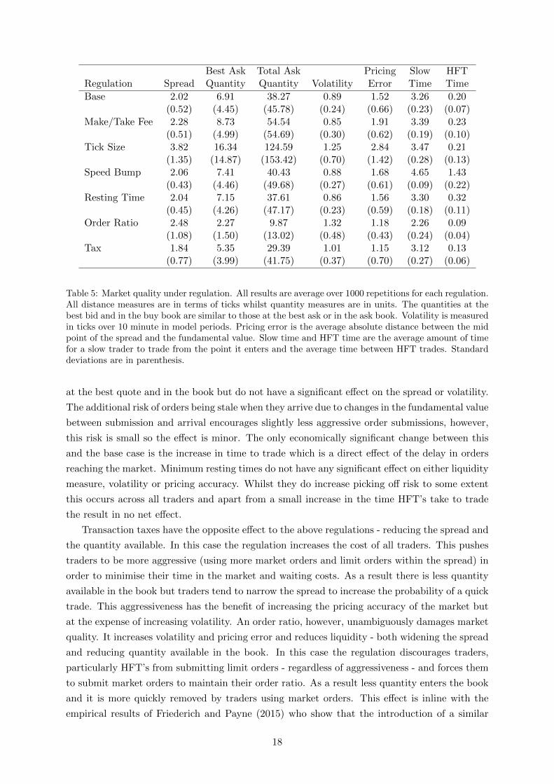
Table 5 shows the effect of the six regulations on market quality. Make take fees and increased

tick sizes have an ambiguous effect on liquidity within the market - widening the spread and

increasing the available quantity. In each case the wider spread increases the costs to using

market orders and trading therefore increasing the use of limit orders, decreasing trade and

increasing the available quantity in the books. Tick sizes do this mechanically be forcing greater

gaps in the price grid. Make take fees, have a similar effect by making it more expensive to

initiate a trade and increasing the incentive to be the limit order supplier relative to the liquidity

taker. The increased preference for limit orders over market orders leads to both slow and HFT

traders spending longer in the market prior to executing. The larger quantities at the quotes

lead to fewer changes in price and therefore lower volatility under make-take fees, however, a

larger tick size mechanically increases this measure. Similarly the reluctance to use market

orders means that the market is slower to track changes in the fundamental price.

Like increases in tick size and make take fees, speed bumps slightly increase available liquidity

17

Best Ask Total Ask Pricing Slow HFTRegulation Spread Quantity Quantity Volatility Error Time Time

Base 2.02 6.91 38.27 0.89 1.52 3.26 0.20(0.52) (4.45) (45.78) (0.24) (0.66) (0.23) (0.07)

Make/Take Fee 2.28 8.73 54.54 0.85 1.91 3.39 0.23(0.51) (4.99) (54.69) (0.30) (0.62) (0.19) (0.10)

Tick Size 3.82 16.34 124.59 1.25 2.84 3.47 0.21(1.35) (14.87) (153.42) (0.70) (1.42) (0.28) (0.13)

Speed Bump 2.06 7.41 40.43 0.88 1.68 4.65 1.43(0.43) (4.46) (49.68) (0.27) (0.61) (0.09) (0.22)

Resting Time 2.04 7.15 37.61 0.86 1.56 3.30 0.32(0.45) (4.26) (47.17) (0.23) (0.59) (0.18) (0.11)

Order Ratio 2.48 2.27 9.87 1.32 1.18 2.26 0.09(1.08) (1.50) (13.02) (0.48) (0.43) (0.24) (0.04)

Tax 1.84 5.35 29.39 1.01 1.15 3.12 0.13(0.77) (3.99) (41.75) (0.37) (0.70) (0.27) (0.06)

Table 5: Market quality under regulation. All results are average over 1000 repetitions for each regulation.All distance measures are in terms of ticks whilst quantity measures are in units. The quantities at thebest bid and in the buy book are similar to those at the best ask or in the ask book. Volatility is measuredin ticks over 10 minute in model periods. Pricing error is the average absolute distance between the midpoint of the spread and the fundamental value. Slow time and HFT time are the average amount of timefor a slow trader to trade from the point it enters and the average time between HFT trades. Standarddeviations are in parenthesis.

at the best quote and in the book but do not have a significant effect on the spread or volatility.

The additional risk of orders being stale when they arrive due to changes in the fundamental value

between submission and arrival encourages slightly less aggressive order submissions, however,

this risk is small so the effect is minor. The only economically significant change between this

and the base case is the increase in time to trade which is a direct effect of the delay in orders

reaching the market. Minimum resting times do not have any significant effect on either liquidity

measure, volatility or pricing accuracy. Whilst they do increase picking off risk to some extent

this occurs across all traders and apart from a small increase in the time HFT’s take to trade

the result in no net effect.

Transaction taxes have the opposite effect to the above regulations - reducing the spread and

the quantity available. In this case the regulation increases the cost of all traders. This pushes

traders to be more aggressive (using more market orders and limit orders within the spread) in

order to minimise their time in the market and waiting costs. As a result there is less quantity

available in the book but traders tend to narrow the spread to increase the probability of a quick

trade. This aggressiveness has the benefit of increasing the pricing accuracy of the market but

at the expense of increasing volatility. An order ratio, however, unambiguously damages market

quality. It increases volatility and pricing error and reduces liquidity - both widening the spread

and reducing quantity available in the book. In this case the regulation discourages traders,

particularly HFT’s from submitting limit orders - regardless of aggressiveness - and forces them

to submit market orders to maintain their order ratio. As a result less quantity enters the book

and it is more quickly removed by traders using market orders. This effect is inline with the

empirical results of Friederich and Payne (2015) who show that the introduction of a similar

18

Slow Traders - 4 Slow Traders - 8 HFT TradersWaiting Waiting

Regulation Cost Profit Cost Profit Profit

Base -0.38 3.44 -0.78 6.86 0.77(0.20) (0.25) (0.37) (0.48) (0.85)

Make/Take Fee -0.47 3.44 -0.96 6.75 0.90(0.21) (0.23) (0.40) (0.45) (1.16)

Tick Size -0.45 3.44 -1.05 6.60 1.48(0.30) (0.48) (0.62) (0.67) (2.31)

Speed Bump -0.47 3.39 -0.95 6.72 0.78(0.17) (0.22) (0.33) (0.44) (0.84)

Minimum Rest -0.40 3.47 -0.81 6.90 0.87(0.17) (0.19) (0.33) (0.38) (0.72)

Order Ratio -0.17 3.58 -0.33 7.28 0.05(0.10) (0.25) (0.15) (0.43) (0.07)

Tax -0.31 2.95 -0.61 6.49 0.42(0.18) (0.23) (0.31) (0.44) (1.07)

Table 6: Gains from trade under regulation. The table shows the average profit per trade for the threegroups of traders: HFT’s, Slow (valuation 4/-4) and Slow (valuation 8/-8). In addition it shows thewaiting cost for each trade, defined as e−ρTα where T is time between entry and trade, i.e. the reductionin potential profits from the private value as a result of time passing between the trader entering themarket and executing the trade. All results are average over 1000 repetitions for each quantity of HFT’s.Standard deviations are shown in parenthesis.

rule in the Italian market harmed liquidity. This differs, however from the findings of Jorgensen

et al. (2018) who show no effect on liquidity for a similar regulation in the Oslo stock exchange.

The principal difference in these two cases is that the latter had features designed to encourage

liquidity provision. The rule we test is much closer to that of the first for which the findings are

in broad agreement.

Table 6 presents the profits of both slow and HFT traders under a range of regulations. As

has previously been suggested by the literature make/take fees benefit HFT’s. In particular

they are able to benefit from the payments for providing liquidity whilst, due to their speed

advantage, they are able to avoid much of the risk. This benefit comes at the expenses of slow

traders, particularly those with the highest value units who obtain lower profits. The immediacy

that these traders typically desire costs them money in the form of market orders fees which are

transferred to HFT’s. Increasing the tick size similarly benefits HFT’s at the expense of slow

traders with high value units. In this case the larger price grid means that the cost of being

picked off increases whilst the benefits to picking another order off similarly increase. This

benefits HFT’s who are better able to avoid the first and exploit the second case.

Speed bumps do not have a positive effect - they reduce the profits of slow traders whilst

leaving HFT’s unaffected. Minimum resting times are beneficial to all traders to some extent.

Small but statistically significant increases in per order profits are observed for both groups of

slow traders whilst HFT’s observe a greater increase in profits. For HFT’s, however, this is

accompanied by an increase in the variance of per order profits. Insisting on minimum resting

times for orders means more opportunities to pick off other traders quote’s and make greater

19

profits. At the same time in some cases HFT’s will have stale orders that will be picked off by

slower traders, or other HFT’s who arrive at the right point in time. Whilst minimum resting

times and speed bumps work in a similar manner, the former is more beneficial to both groups of

traders. This difference is due to where the delay occurs. In the case of speed bumps it is prior

to the order arriving at the market - effectively increasing waiting costs, whilst for minimum

resting times the same delay in arrival is not present.

If the focus of regulation were to drive high frequency traders from markets, despite their

positive effects, transaction taxes and order ratio’s both reduce profits for this group. Transac-

tion taxes do this by increasing the cost to trading. This negatively effects HFT’s by reducing

or completely eliminating the small profits they make on each order. This same effect, however,

also applies to slow traders and reduces the profits of non HFT traders by a greater amount.

Order ratio’s in contrast have the dual advantage of slightly increasing non-HFT trader profits

whilst making HFT trading almost completely unprofitable. The order ratio makes the normal

strategy of HFT’s based on rapidly adjusting limit orders impossible to maintain. The require-

ment to make a fraction of trades relative to orders effectively eliminates their ability to use

speed to provide the best quotes at all times. This regulatory change completely negates the

advantage of HFT traders. The order ratio has little direct effect on non-HFT’s as they typically

use market orders more frequently. This would therefore appear to be a very effective tool in

regulating HFT’s profits but with the non-trivial effects on market quality noted above.

6 Conclusion

The theoretical analysis of high frequency trading has generally focused on optimal behaviour,

and so has ignored the trade-off between sophisticated decision making and time. I present a

model of the interaction of high frequency traders in which trading speed is dictated by strategy

sophistication and the choice of strategy sophistication is endogenous. Using this model I show

that there are multiple equilibria in strategy design. Despite competition to be first by being

quickest, traders adopt a range of sophistication’s with short strategies making large numbers

of low profit trades and more sophisticate strategies identifying a smaller number of high profit

trades. A suite of regulations proposed to limit the negative effects of HFT’s are shown to

generally be ineffective in either improving market quality or reducing the profits of HFT’s. The

only exception is that of a ratio for the number of trades to orders, this may benefit slow traders

at the expense of HFT’ but with some negative consequences on the market as a whole.

20

References

Bernales, A., 2016. Algorithmic and high frequency trading in dynamic limit order markets.

Tech. rep., SSRN.

Biais, B., Foucault, T., Moinas, S., 2015. Equilibrium fast trading. Journal of Financial Eco-

nomics 116 (2), 292–313.

Breaban, A., Noussair, C. N., 2015. Trader characteristics and fundamental value trajectories

in an asset market experiment. Journal of Behavioral and Experimental Finance 8, 1 – 17.

Brogaard, J., Hagstrmer, B., Nordn, L., Riordan, R., 2015. Trading fast and slow: Colocation

and liquidity. The Review of Financial Studies 28 (12), 3407–3443.

Brogaard, J., Hendershott, T., Riordan, R., 2014. High-frequency trading and price discovery.

The Review of Financial Studies 27 (8), 2267–2306.

Budish, E., Cramton, P., Shim, J., 2015. The High-Frequency Trading Arms Race: Frequent

Batch Auctions as a Market Design Response. The Quarterly Journal of Economics 130 (4),

1547–1621.

Burks, S. V., Carpenter, J. P., Goette, L., Rustichini, A., 2009. Cognitive skills affect economic

preferences, strategic behavior, and job attachment. Proceedings of the National Academy of

Sciences 106 (19), 7745–7750.

Chen, S.-H., Tai, C.-C., Yang, L.-X., 2017. Cognitive capacity and earnings performance: Evi-

dence from double auction market experiments. Tech. rep., mimeo.

Chen, Y., Wang, X., 2015. A hybrid stock trading system using genetic network programming

and mean conditional value-at-risk. European Journal of Operational Research 240 (3), 861 –

871.

Chiarella, C., Ladley, D., 2016. Chasing trends at the micro-level: The effect of technical trading

on order book dynamics. Journal of Banking & Finance 72 (S), 119–131.

Corgnet, B., Hernan-Gonzalez, R., Kujal, P., Porter, D., 2015. The effect of earned versus house

money on price bubble formation in experimental asset markets. Review of Finance 19 (4),

1455–1488.

Coval, J. D., Hirshleifer, D., Shumway, T. G., Dec. 2004. Can Individual Investors Beat the

Market? Finance 0412005, EconWPA.

Delaney, L., 2018. Investment in high-frequency trading technology: A real options approach.

European Journal of Operational Research 270 (1), 375 – 385.

Foucault, T., Kadan, O., Kandel, E., 2013. Liquidity cycles and make/take fees in electronic

markets. The Journal of Finance 68 (1), 299–341.

Foucault, T., Kozhan, R., Tham, W. W., 2017. Toxic Arbitrage. Review of Financial Studies

30 (4), 1053–1094.

21

Friederich, S., Payne, R., 2015. Order-to-trade ratios and market liquidity. Journal of Banking

& Finance 50, 214 – 223.

Goettler, R. L., Parlour, C. A., Rajan, U., 2009. Informed traders and limit order markets.

Journal of Financial Economics 93 (1), 67 – 87.

Grinblatt, M., Keloharju, M., Linnainmaa, J. T., 2012. IQ, trading behavior, and performance.

Journal of Financial Economics 104 (2), 339–362.

Hagstromer, B., Norden, L., 2013. The diversity of high-frequency traders. Journal of Financial

Markets 16 (4), 741 – 770.

Hendershott, T., Jones, C. M., Menkveld, A., 2011. Does algorithmic trading improve liquidity?

Journal of Finance 66 (1), 1–33.

Hollifield, B., Miller, R. A., Sandas, P., Slive, J., 2006. Estimating the gains from trade in

limit-order markets. The Journal of Finance 61 (6), 2753–2804.

Jorgensen, K., Skjeltorp, J., degaard, B. A., 2018. Throttling hyperactive robots order-to-trade

ratios at the oslo stock exchange. Journal of Financial Markets 37, 1 – 16.

Kirilenko, A., Kyle, A. S., Samadi, M., Tuzun, T., 2017. The flash crash: High-frequency trading

in an electronic market. The Journal of Finance 72 (3), 967–998.

Korajczyk, R. A., Murphy, D., 07 2018. High-Frequency Market Making to Large Institutional

Trades. The Review of Financial Studies 32 (3), 1034–1067.

Ladley, D., Lensberg, T., Palczewski, J., Schenk-Hopp, K. R., 2015. Fragmentation and stability

of markets. Journal of Economic Behavior & Organization 119 (C), 466–481.

Leal, S. J., Napoletano, M., 2017. Market stability vs. market resilience: Regulatory policies ex-

periments in an agent-based model with low- and high-frequency trading. Journal of Economic

Behavior and Organization.

Lensberg, T., Schenk-Hopp, K. R., Ladley, D., 2015. Costs and benefits of financial regulation:

Short-selling bans and transaction taxes. Journal of Banking and Finance 51, 103 – 118.

Manahov, V., Soufian, M., Hudson, R., 01 2014. The Implications Of Trader Cognitive Abilities

On Stock Market Properties. Intelligent Systems in Accounting, Finance and Management

21 (1), 1–18.

Menkveld, A., Zoican, M. A., 2017. Need for Speed? Exchange Latency and Liquidity. Post-Print

hal-01501352, HAL.

Menkveld, A. J., 2013. High frequency trading and the new market makers. Journal of Financial

Markets 16 (4), 712 – 740.

Menkveld, A. J., October 2016. The Economics of High-Frequency Trading: Taking Stock.

Annual Review of Financial Economics 8 (1), 1–24.

22

Moore, H. L., 1911. Laws of wages; an essay in statistical economics. New York: The Macmillan

Company.

Neely, C., Weller, P., Dittmar, R., 1997. Is technical analysis in the foreign exchange market

profitable? a genetic programming approach. Journal of Financial and Quantitative Analysis

32 (4), 405426.

Noussair, C. N., Tucker, S., Xu, Y., 2016. Futures markets, cognitive ability, and mispricing in

experimental asset markets. Journal of Economic Behavior & Organization 130 (C), 166–179.

Paulin, J., Calinescu, A., Wooldridge, M., 2019. Understanding flash crash contagion and sys-

temic risk: A micromacro agent-based approach. Journal of Economic Dynamics and Control

100, 200 – 229.

Riordan, R., Storkenmaier, A., 2012. Latency, liquidity and price discovery. Journal of Financial

Markets 15 (4), 416 – 437.

Turner, A. J., Miller, J. F., 2014. Introducing a cross platform open source cartesian genetic

programming library. The Journal of Genetic Programming and Evolvable Machines 16, 83–

91.

Yeh, C.-H., 2008. The effects of intelligence on price discovery and market efficiency. Journal of

Economic Behavior and Organization 68 (3), 613 – 625.

Yeh, C.-H., Yang, C.-Y., 2010. Examining the effectiveness of price limits in an artificial stock

market. Journal of Economic Dynamics and Control 34 (10), 2089 – 2108.

23