Fast Quadrature Te hniques for RetardedPotentials Based on TT/QTT TensorApproximationB. N. Khoromskij∗ S. Sauter† A. Veit‡§Abstra tWe onsider the Galerkin approa h for the numeri al solution of retarded boundaryintegral formulations of the three dimensional wave equation in unbounded domains.Re ently smooth and ompa tly supported basis fun tions in time were introdu edwhi h allow the use of standard quadrature rules in order to ompute the entries of theboundary element matrix. In this paper we use TT and QTT tensor approximations toin rease the e ien y of these quadrature rules. Various numeri al experiments showthe substantial redu tion of the omputational ost that is needed to obtain a urateapproximations for the arising integrals.AMS Subje t Classi ation: 65F30, 65F50, 65N38, 65F10Key words: Multi-dimensional problems, tensor approximation, quantized representation ofve tors, model redu tion, retarded potentials, 3D wave equation, quadrature rules.1 Introdu tionA ousti and ele tromagneti s attering problems in three dimensions have a wide rangeof pra ti al appli ations in physi s and engineering. An important model problem for thedevelopment of e ient and a urate numeri al methods for su h types of time-dependentphysi al appli ations is the three-dimensional wave equation in unbounded exterior domains.Here, boundary element methods show their natural strength, redu ing the problem in theunbounded domain to integral equations on the bounded surfa e of the s atterer.The e ient numeri al solution of su h retarded boundary integral equations has gainedgrowing attention in the last years. Existing approa hes in lude methods based on onvo-lution quadrature ( f. [3, 4, 5, 11, 12) and methods based on bandlimited interpolationand extrapolation ( f. [32, 33, 34, 36). Here, we onsider a Galerkin method in order to

∗(bokhmis.mpg.de)Max-Plan k-Institut für Mathematik in den Naturwissens haften, Inselstr. 22-26,04103 Leipzig, Germany†(stasmath.uzh. h), Institut für Mathematik, Universität Züri h, Winterthurerstr. 190, CH-8057 Züri h,Switzerland‡(alexander.veitmath.uzh. h), Institut für Mathematik, Universität Züri h, Winterthurerstr. 190, CH-8057 Züri h, Switzerland§The third author gratefully a knowledges the support given by SNF, No. PDFMP2_127437/11

dis retize the integral equations in spa e and time ( f. [2, 6, 8, 9). It an be shown thatthe orresponding spa e-time variational formulation in this approa h satises a oer ivityproperty whi h ensures the un onditional stability of onforming Galerkin s hemes. Fur-thermore, this approa h is very exible with regard to the use of variable time steppingand spatially urved s atterers. The standard Galerkin approa h uses pie ewise polynomialbasis fun tions in time. The drawba k of the method in this ase is that due to the retardedtime argument the domain for the spatial integration is the interse tion of (possibly urved)pairs of surfa e panels with the dis rete light one. The stable numeri al handling of theseinterse tions is ompli ated even for at panels and might be intra table for urved surfa epat hes. We refer to [7, 21, 29 for examples of quadrature s hemes tailored to this problem.In [26 smooth and ompa tly supported basis fun tions in time were introdu ed. This hoi e ir umvents the problem of integrating on the ompli ated interse tions of the dis- rete light one with the spatial surfa e mesh and allows to apply standard quadrature rulesto ompute the entries of the boundary element matrix. Due to the ompa t support of thebasis fun tions the sparsity of the system matrix is maintained. On the other hand this leadsto C∞ but, in general, non-analyti integrands, whi h makes the quadrature problem moredi ult. In general, more quadrature points have to be used as for analyti integrands asthey arise, e.g., for boundary element methods applied to ellipti boundary value problems.In this paper we therefore address the problem how to e iently evaluate the arising inte-grals using tensor Gauss quadrature and TT/QTT approximation. Note, that other te h-niques su h as sparse, possibly adaptive quadrature also have the potential to be appliedto this problem. Preliminary test with sparse grid quadrature indi ates, that our TT/QTTapproa h is preferable for this lass of problems, espe ially if high a ura ies are needed.However an asymptoti omplexity analysis still has to be done.The integrals whi h dene the entries of the blo k system matrix are dened over pairs ofsurfa e panels. They are transformed to the referen e triangle in Eu lidean spa e and byapplying simplex oordinates the quadrature problems boils down to the approximation ofan integral over the four-dimensional unit ube. A tensor quadrature rule applied to theseintegrals leads to a four dimensional tensor A of size N × N × N × N , whose entries arethe values of the integrand evaluated at the dierent quadrature points.To redu e the storage and omputational osts to handle this large data array, we applythe methods of tensor approximation based on the idea of separation of variables. Thereare various tensor-produ t formats whi h allow the low parametri representation of high-dimensional data. The most ommonly used are the anoni al, Tu ker formats as well asthe lass of so- alled matrix produ t states (MPS) representations [35, 30, 31 ommonlyused in high-dimensional quantum omputations (see survey paper [16 for more details).Re ently these types of tensor formats have attra ted mu h attention in the ommunity ofnumeri al analysis. In parti ular, the hierar hi al Tu ker [13, the tensor train (TT) [23and the tensor hain (TC) [17 formats were onsidered. In the following we make useof the TT format applied to both the initial fourth order tensor and to its quantized-TT(QTT) representation. Su h representations allow to redu e the asymptoti al storage and omputational osts of ertain bilinear tensor operations from O(N4) to O(r2N) or evento O(r2 logN) (avoiding the dependen e on the grid-size), where r is the small rank pa-rameter, hara terizing the separability properties of the target tensor A. Noti e that thehierar hi al Tu ker format was re ently applied in the same spirit to omputation of ertainmultivariate integrals arising in boundary element methods [1.Various numeri al experiments show that these tensors have usually a low rank represen-2

tation in TT and QTT format whi h redu es the storage and omputational ost substan-tially. The evaluation of the quadrature then orresponds to a simple s alar produ t of theTT/QTT representation of A and a rank-1 tensor ontaining the weights of the quadraturerule. This evaluation an be performed onsiderably faster ompared to the standard ap-proa h. In order to ompute the TT/QTT approximation of A dire tly, without omputingA itself, we apply a TT ross approximation s heme ( f. [24) in the QTT format. Thisfurther redu es the omputational ost, sin e onsiderably less evaluations of the integrandare required. We perform numeri al experiments to show the e ien y of this s heme inour ase.Note that our sparse approximation method for high-dimensional quadrature problems isby no means restri ted to the retarded potential integral equation but, potentially, anbe applied to a mu h larger lass of problems. We restri ted to this appli ation be ausequadrature is the major bottlene k for the dire t dis retization of retarded potentials.2 Problem SettingLet Ω ⊂ R

3 be a Lips hitz domain with boundary Γ. We onsider the homogeneous waveequation∂2t u−∆u = 0 in Ω× [0, T ] (2.1a)with initial onditionsu(·, 0) = ∂tu(·, 0) = 0 in Ω (2.1b)and Diri hlet boundary onditions

u = g on Γ× [0, T ] (2.1 )on a time interval [0, T ] for T > 0. In appli ations, Ω is often the unbounded exterior ofa bounded domain. For su h problems, the method of boundary integral equations is anelegant tool where this partial dierential equation is transformed to an equation on thebounded surfa e Γ. We employ an ansatz as a single layer potential for the solution uu(x, t) := Sφ(x, t) :=

∫

Γ

φ(y, t− ‖x− y‖)

4π‖x− y‖dΓy, (x, t) ∈ Ω× [0, T ] (2.2)with unknown density fun tion φ. S is also referred to as retarded single layer potential dueto the retarded time argument t− ‖x− y‖ whi h onne ts time and spa e variables.The ansatz (2.2) satises the wave equation (2.1a) and the initial onditions (2.1b). Sin ethe single layer potential an be extended ontinuously to the boundary Γ, the unknowndensity fun tion φ is determined su h that the boundary onditions (2.1 ) are satised. Thisresults in the boundary integral equation for φ,

∫

Γ

φ(y, t− ‖x− y‖)

4π‖x− y‖dΓy = g(x, t) ∀(x, t) ∈ Γ× [0, T ] . (2.3)In order to solve this boundary integral equation numeri ally we introdu e the followingspa e-time variational formulation ( f. [2, 8): Find φ in an appropriate Sobolev spa e Vsu h that

∫ T

0

∫

Γ

∫

Γ

φ(y, t− ‖x− y‖)ζ(x, t)

4π‖x− y‖dΓydΓxdt =

∫ T

0

∫

Γg(x, t)ζ(x, t)dΓxdt (2.4)3

for all ζ ∈ V , where we denote by φ the derivative with respe t to time.Let VGalerkin be a nite dimensional subspa e of V being spanned by L basis fun tionsbi

Li=1 in time and M basis fun tions ϕj

Mj=1 in spa e. This leads to the fully dis reteansatz

φGalerkin(x, t) =

L∑

i=1

M∑

j=1

αjiϕj(x)bi(t), (x, t) ∈ Γ× [0, T ] , (2.5)where αj

i are the unknown oe ients. Plugging this ansatz in (2.4) and rearranging termsshows that this is equivalent to: Find αji for i = 1, . . . , L and j = 1, . . . ,M su h that

L∑

i=1

M∑

j=1

Ai,kj,lα

ji = gkl ∀1 ≤ k ≤ L ∀1 ≤ l ≤M, (2.6)where

gkl :=

∫ T

0

∫

Γg(x, t)ϕl(x) bk(t)dΓxdtand

Ai,kj,l :=

∫

supp(ϕl)

∫

supp(ϕj)ϕj(y)ϕl(x)ψi,k(‖x− y‖)dΓydΓx. (2.7)The fun tion ψi,k ontains the time integration and is dened, for s > 0, by

ψi,k(s) :=

∫ T

0

bi(t− s)bk(t)

4πsdt. (2.8)Let G :=

τi : 1 ≤ i ≤M

denote a nite element mesh on Γ onsisting of (possibly urved)triangles. More pre isely, we assume that for any τ ∈ G, there exists a smooth bije tionχτ : τ → τ from the referen e element τ := conv (0, 0)⊺ , (1, 0)⊺ , (1, 1)⊺ to the surfa etriangle τ . Then, in the solution pro ess, the following quadrature problem arises: Forτ, τ ∈ G and 1 ≤ j, l ≤M , ompute

Ii,kτ,τ (ϕj , ϕl) :=

∫

τ

∫

τϕj(y)ϕl(x)ψi,k(‖x− y‖)dΓydΓx, (2.9)where ϕj and ϕl, typi ally, are lifted polynomials, i.e., ϕj χτ and ϕl χτ are polynomialson τ .The denition of smooth and ompa tly supported temporal shape fun tions was ad-dressed in [26 and is as follows. Let

f (t) :=

12 erf (2 artanh t) +

12 |t| < 1,

0 t ≤ −1,1 t ≥ 1and note, that f ∈ C∞ (R). Next, we will introdu e some s aling. For a fun tion g ∈

C0 ([−1, 1]) and real numbers a < b, we dene ga,b ∈ C0 ([a, b]) byga,b (t) := g

(2t− a

b− a− 1

).4

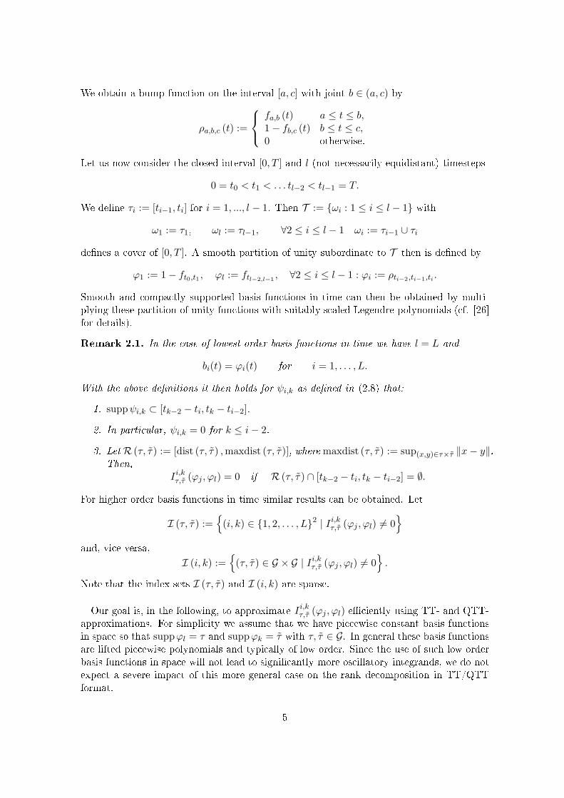
We obtain a bump fun tion on the interval [a, c] with joint b ∈ (a, c) byρa,b,c (t) :=

fa,b (t) a ≤ t ≤ b,

1− fb,c (t) b ≤ t ≤ c,

0 otherwise.Let us now onsider the losed interval [0, T ] and l (not ne essarily equidistant) timesteps0 = t0 < t1 < . . . tl−2 < tl−1 = T.We dene τi := [ti−1, ti] for i = 1, ..., l − 1. Then T := ωi : 1 ≤ i ≤ l − 1 with

ω1 := τ1, ωl := τl−1, ∀2 ≤ i ≤ l − 1 ωi := τi−1 ∪ τidenes a over of [0, T ]. A smooth partition of unity subordinate to T then is dened byϕ1 := 1− ft0,t1 , ϕl := ftl−2,l−1

, ∀2 ≤ i ≤ l − 1 : ϕi := ρti−2,ti−1,ti .Smooth and ompa tly supported basis fun tions in time an then be obtained by multi-plying these partition of unity fun tions with suitably s aled Legendre polynomials ( f. [26for details).Remark 2.1. In the ase of lowest order basis fun tions in time we have l = L andbi(t) = ϕi(t) for i = 1, . . . , L.With the above denitions it then holds for ψi,k as dened in (2.8) that:1. suppψi,k ⊂ [tk−2 − ti, tk − ti−2].2. In parti ular, ψi,k = 0 for k ≤ i− 2.3. LetR (τ, τ) := [dist (τ, τ) ,maxdist (τ, τ)], where maxdist (τ, τ) := sup(x,y)∈τ×τ ‖x− y‖.Then,

Ii,kτ,τ (ϕj , ϕl) = 0 if R (τ, τ ) ∩ [tk−2 − ti, tk − ti−2] = ∅.For higher order basis fun tions in time similar results an be obtained. Let

I (τ, τ ) :=(i, k) ∈ 1, 2, . . . , L2 | Ii,kτ,τ (ϕj , ϕl) 6= 0

and, vi e versa,I (i, k) :=

(τ, τ) ∈ G × G | Ii,kτ,τ (ϕj , ϕl) 6= 0

.Note that the index sets I (τ, τ) and I (i, k) are sparse.Our goal is, in the following, to approximate Ii,kτ,τ (ϕj , ϕl) e iently using TT- and QTT-approximations. For simpli ity we assume that we have pie ewise onstant basis fun tionsin spa e so that suppϕl = τ and suppϕk = τ with τ, τ ∈ G. In general these basis fun tionsare lifted pie ewise polynomials and typi ally of low order. Sin e the use of su h low orderbasis fun tions in spa e will not lead to signi antly more os illatory integrands, we do notexpe t a severe impa t of this more general ase on the rank de omposition in TT/QTTformat. 5

Be ause simplex oordinates transform triangles to squares, integrals of the form (2.9) anbe written as∫

τ

∫

τψi,k (‖x− y‖) dΓydΓx = (2.10)∫

[0,1]44|τ ||τ |ξxξy ψi,k(‖χτ (ξx, ξxηx)− χτ (ξy, ξyηy)‖)︸ ︷︷ ︸

=:f(ξx,ηx,ξy,ηy)

dηydξydηxdξx.We apply properly s aled tensor Gauss-Legendre quadrature rules for the numeri al approx-imation of the arising integrals over the four-dimensional unit ube. Let n1, n2, n3, n4 ∈ N>0be the number of Gauss quadrature points in the rst/se ond/third/fourth dimension withnodes(x1,i)

n1

i=1, (x2,j)n2

j=1, (x3,k)n3

k=1, (x4,l)n4

l=1 ∈ [0, 1]and weights(w1,i)

n1

i=1, (w2,j)n2

j=1, (w3,k)n3

k=1, (w4,l)n4

l=1 ∈ R.Then,∫

[0,1]4f(ξx, ηx, ξy, ηy) dηydξydηxdξx ≈

n1∑

i=1

n2∑

j=1

n3∑

k=1

n4∑

l=1

w1,iw2,jw3,kw4,lf(x1,i, x2,j , x3,k, x4,l).(2.11)For simpli ity and in order to test the QTT approximation we set n1 = n2 = n3 =n4 =: N and assume that N is a power of 2. The evaluation of an approximation inthe form (2.11) requires O(N4) additions/multipli ations and furthermore O(N4) fun tionevaluations. Sin e f , or more spe i ally ψi,k, ontains itself an integral, su h fun tionevaluations might be expensive. Due to the non-analyti ity of f and the need to ompute theintegrals (2.10) a urately in order to obtain stable solutions of the time-domain boundaryintegral equations, we need a medium number of quadrature points in ea h dire tion. Thus,depending on the required a ura y of the approximation, the quadrature problem anbe ome ostly. Therefore the question arises if the right hand side in (2.11) an be evaluatedmore e iently. For this purpose we will investigate, in the following, the TT and QTT lowrank approximations to the fourth order tensor A = [A(i, j, k, l)] dened entrywise by

A(i, j, k, l) = f(x1,i, x2,j, x3,k, x4,l), (i, j, k, l) ∈ 1, ..., N4. (2.12)Note that for the singular ase, where dist (τ, τ ) = 0, regularizing oordinate transformshave to be applied to remove the singularity of the kernel fun tion ( f. [28, [25). In this ase, the transformed integral is a sum of integrals over the four-dimensional unit ube andour ompression method an be applied also to these ases. For simpli ity we restri t inthis paper to the approximation of the regular integrals.3 Tensor Approximation of I i,jτ,τ (ϕj, ϕl)In the following we apply the matrix-produ t states (MPS) type tensor representations in theform of tensor train (TT) and quantized-TT (QTT) formats to represent sparsely the fourthorder oe ients tensor arising in the quadrature approximation of the above integrals (see(2.11)). 6

3.1 Matrix-produ t states (MPS) tensor formatsA tensor of order d is dened as an element of nite dimensional tensor-produ t Hilbert spa eWn ≡ W

n,d of the d-fold, N1 × ...×Nd real-valued arrays, and equipped with the Eu lidean(Frobenius) s alar produ t 〈·, ·〉 : Wn ×Wn → R. Ea h tensor in Wn, n = (N1, ..., Nd), anbe represented omponentwise,A = [A(i1, ..., id)] with iℓ ∈ Iℓ := 1, ..., Nℓ,where for the ease of presentation, we mainly onsider the equal-size tensors, i.e., Nℓ = N(ℓ = 1, ..., d). We all the elements of Wn = R

I1×...×Id as N -d tensors. The dimension ofthe tensor-produ t Hilbert spa e Wn s ales exponentially in d, dim Wn,d = Nd implyingexponential storage ost for a general N -d tensor.In our appli ation the quadrature oe ients for approximating Ii,kτ,τ (ϕj, ϕl) onstitutethe N ×N ×N ×N tensor A of order 4 as in (2.12), requiring N4 storage size. Hen e, inthe ase of multiple omputations of a tensor and high numeri al ost of evaluation a singleentry, the al ulations be ome nontra table already for N of order several tens.The MPS representation of a d-th order tensor redu es the omplexity of storage to

O(dr2N), where r is the maximal mode rank [35, 30. The MPS tensor approximationwas proved to be e ient in high-dimensional ele troni /mole ular stru ture al ulations,in quantum omputing and in sto hasti PDEs (see survey paper [16 for more details). Inthe re ent mathemati al literature the various versions of MPS tensor de omposition weredis overed as the hierar hi al Tu ker [13, the tensor train (TT) [23 and the tensor hain(TC) [17 formats. In the following we make use of the TT format applied to both the initialN -d tensor and to its quantized representation (quanti s-TT).Denition 3.1. (Tensor hain/train format) For a given rank parameter r = (r0, ..., rd),and the respe tive index sets Jℓ = 1, ..., rℓ (ℓ = 0, 1, ..., d), with the periodi ity onstraintsJ0 = Jd (i.e., r0 = rd), the rank-r TC format ontains all elements A = [A(i1, ..., id)] ∈ Wnwhi h an be represented as the hain of ontra ted produ ts of 3-tensors over the d-foldprodu t index set J := ×d

ℓ=1Jℓ,A(i1, ..., id) =

∑

α1∈J1

· · ·∑

αd∈Jd

A(1)(αd, i1, α1)A(2)(α1, i2, α2) · · ·A

(d)(αd−1, id, αd).In the matrix form we have the entrywise MPS representationA(i1, i2, . . . , id) = A

(1)i1A

(2)i2. . . A

(d)id, (3.1)where ea h A(ℓ)

iℓis rℓ−1 × rℓ matrix. In the ase J0 = Jd = 1, the TC format oin ideswith TT representation in [23.The TC/TT format redu es the storage ost of a N -d tensor to O(dr2N), r = max rℓ.The important multilinear algebrai operations with TT tensors an be implemented withlinear omplexity s aling in d and N . In parti ular, for the Hadamard produ t we have

Z = X Y : Z(k)(ik) = X(k)(ik)⊗ Y (k)(ik),implying the formatted representation of the s alar produ t (in O(dr3N) ≪ Nd operations)〈X,Y〉 = 〈X Y,1〉.7

3.2 Quantized-TT (QTT) Approximation of N-d tensorsFurther redu tion of the asymptoti storage omplexity an be based on the so- alledquantized-TT (QTT) representation obtained from the initial N × N × N × N tensor bysimple folding (reshaping) to higher dimensional 2× ...× 2 array. It was shown in [17 thatthe omputational gain of the QTT representation is due to the good separability propertiesof quantized images on a large lass of fun tion related tensors. In our appli ation we foundnumeri ally the low rank TT/QTT approximations for arising 4th order tensors, indi atingnearly the same data ompression for both formats. However, the important motivation touse the QTT representation is due to the high e ien y of the QTT- ross approximations heme ensured by the small mode size (in fa t, equals to 2) of the quantized tensors.We suppose that N = 2L with some L = 1, 2, . . . . The next denition introdu es thefolding of N -d tensors into the elements (quantized 2 × ... × 2 tensors) of an auxiliaryD-dimensional tensor spa e with D = d log2N .Denition 3.2. ([17) Introdu e the binary folding transform of degree 2 ≤ L,

Fd,L : Wn,d → W

m,dL, m = (m1, ...,md), mℓ = (mℓ,1, ...,mℓ,L),with mℓ,ν = 2 for ν = 1, ..., L, (ℓ = 1, ..., d), that reshapes the initial n-d tensor in Wn,d toelements of the quantized spa e W

m,dL as follows:(A) For d = 1 a ve tor X = [X(i)]i∈I ∈ WN,1, is reshaped to the element of W2,L byF1,L : X → Y = [Y (j)] := [X(i)], j = j1, ..., jL,with jν ∈ 1, 2 for ν = 1, ..., L. For xed i, jν = jν(i) is dened by jν − 1 = C−1+ν , wherethe C−1+ν are found from the binary representation of i− 1,

i− 1 = C0 + C121 + · · ·+ CL−12

L−1 ≡L∑

ν=1

(jν − 1)2ν−1.(B) For d > 1 the onstru tion is similar.Noti e that the folding transform Fd,L is the linear isometry between WN,d and W2,dL(see [17).Remark 3.3. Every 2-dL tensor in the quanti s spa e W2,dL an be represented (approxi-mated) in the low rank TT format. This leads to the so- alled QTT representation of N -dtensors. Assuming that rk ≤ r, k = 1, ..., dL, the omplexity of the QTT representation anbe estimated by O(dr2 logN), providing log-volume asymptoti s ompared with the volumesize of the initial tensor O(Nd).3.3 Sket h of numeri al TT/QTT approximationThe manifold [14 of rank-r TT tensors in Wn is known to be losed in the Frobenius norm[24.>From the omputational point of view, one of the most attra tive features of TT for-mat is the following: the numeri al omputation of rk−1 × rk matri es A(k)ik

in the TTrepresentation (approximation) of a full format tensor A = [A(i1, ..., id)],A(i1, i2, . . . , id) = A

(1)i1A

(2)i2. . . A

(d)id,8

an be implemented by a stable SVD-based algorithm (MATLAB Toolbox http://spring.inm.rus.ru/osel). For the ompleteness of presentation, we sket h the full-to-TT om-pression algorithm [23, whi h will be applied in Se tion 4 to our parti ular fourth order oe ients tensor.Input: a tensor A of size n1 × n2 · · · × nd and a ura y bound ε > 0.1: First unfolding: Nr =∏d

k=2 nk, M := reshape(A, [n1, Nr]).2: Compute the trun ated SVD of M ≈ UΛV , so that the approximate rank r ensuresmin(n1,Nr)∑

k=r+1

σ2k ≤(ε · ‖A‖F )

2

d− 1.3: Set A(1) = U , M := ΛV T , r1 = r, and pro ess modes k = 2, ..., d − 1.4: for k = 2 to d− 1 do4a: Constru t the next unfolding: Nr :=

Nr

nk, M := reshape(M, [rnk, Nr]).4b: Compute the trun ated SVD of M ≈ UΛV , so that the approximate rank r ensures

min(nk ,Nr)∑

k=r+1

σ2k ≤(ε · ‖A‖F )

2

d− 1.4 : Set rk = r and reshape the matrix U into a tensor:

A(k) := reshape(U, [rk−1, nk, rk]).4d: Re ompute M := ΛV .end for5: Set A(d) =M .Output: TT ores Ak, k = 1, . . . d, dening a TT ε-approximation to A.The above algorithm has the numeri al omplexity O(nd+1). In the present paper we di-re tly apply this algorithm to the fourth-order tensor of interest to demonstrate the e ientrank de omposition in the TT format that redu es drasti ally the storage and omputa-tional ost. Moreover, assuming the existen e of low-rank TT representation the rank-rTT approximation an be omputed by the heuristi algorithm alled TT- ross approxima-tion [24 avoiding the urse of dimensionality (see the numeri al example below). Thisalgorithm also applies to QTT format (QTT- ross approximation).Remark 3.4. Noti e that the QTT approximation of the target N ×N ×N ×N tensor A an be performed by the same de omposition algorithm but applied in the parti ular settingnk = 2, d = 4 logN . The rank-r QTT- ross approximation takes the advantage of low ost O(r4 logN) sin e, due to the main property of TT- ross algorithm, it alls only forO(r2 logN) entries of the initial tensor A. In this way, the generation of the full tensor anbe avoided by using the rank-r QTT- ross approximation method that requires to omputeonly few entries ( hosen adaptively) of the target tensor. The numeri al results show thatthe ompression is omparable with the omplete QTT approximation method (see Se tion4.6). 9

3.4 Computation of I i,jτ,τ (ϕj, ϕl) using TT/QTT approximationLet us denote the TT and QTT representations of A, dened in (2.12), by ATT and AQTT .An approximation of the integral in (2.11) using these representations instead of A anbe obtained by a simple tensor operation in the quanti s spa e W2,dL, d = 4, L = logN ,spe i ally as the s alar produ t of the rank-1 oe ients tensor W = w1 ⊗ w2 ⊗ w3 ⊗ w4with ATT or AQTT . LetQG := 〈W,A〉 =

N∑

i=1

N∑

j=1

N∑

k=1

N∑

l=1

w1,iw2,jw3,kw4,lf(x1,i, x2,j , x3,k, x4,l), (3.2)QTT := 〈W,ATT 〉, (3.3)QQTT := 〈W,AQTT 〉, (3.4)denote the quadrature formulas based on the dierent representations of A. As pointed outin Se tion 3.1 the ost to evaluate the s alar produ ts QTT or QQTT s ales with O(4r3N),where r is mu h smaller than N , ompared to O(N4) for the exa t evaluation of QG. There-fore the approximations QTT and QQTT an be omputed onsiderably faster, provided that

A has TT and QTT representations with low rank.Sin e ATT and AQTT are only approximations of A, the formulas QTT and QQTT intro-du e additional quadrature errors. An important question therefore is how a urate theapproximations ATT/QTT have to be, su h that the relative errorsEG,TT :=

|QG −QTT |

|QG|and EG,QTT :=

|QG −QQTT |

|QG|(3.5)are small and the additional error does not ae t the a ura y of the quadrature QG.4 Numeri al ExperimentsIn the following, we investigate the ompression properties of A and the a ura y of QTTand QQTT using dierent triangles and time meshes in order to over various ases, thatmight o ur during the solution of the dis rete system (2.6) . Therefore, let

τ := conv(0, 0, 0)T, (1, 0, 0)T , (1, 1, 0)T

,

τ := cshift + conv

(1, 0, 0)T, (1, 1

2, 1)T , (0, 1,

1

2)T

,with cshift ∈ R. These triangles will be used for all numeri al experiments. Only cshift ∈ Ris variable and will be set individually for ea h ase. Furthermore we will dene dierenttime grids for ea h ase onsisting of six points t1 ≤ . . . ≤ t6 ∈ R≥0. We then hoose basisfun tion b(t) and b(t) in time su h that supp b = [t1, t3] and supp b = [t4, t6]. More pre isely,b and b will be the smooth bump fun tions as dened in Se tion 2 multiplied with properlys aled Legendre polynomials of degree 1 ( f. [26), i.e.,

b(t) = ρt1,t2,t3(t)

(2t− t1

t3 − t1− 1

) and b(t) = ρt4,t5,t6(t)

(2t− t4

t6 − t4− 1

). (4.1)Thus, the integrals we want to approximate are of the form

Iτ,τ :=

∫

τ

∫

τψ (‖x− y‖) dΓydΓx, (4.2)10

8.5 9 9.5 10−0.2

−0.15

−0.1

−0.05

0

0.05

0.1

0.15

0.2

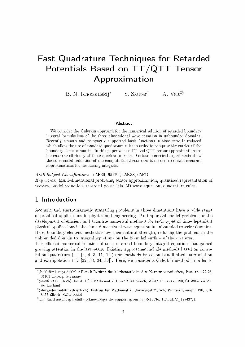
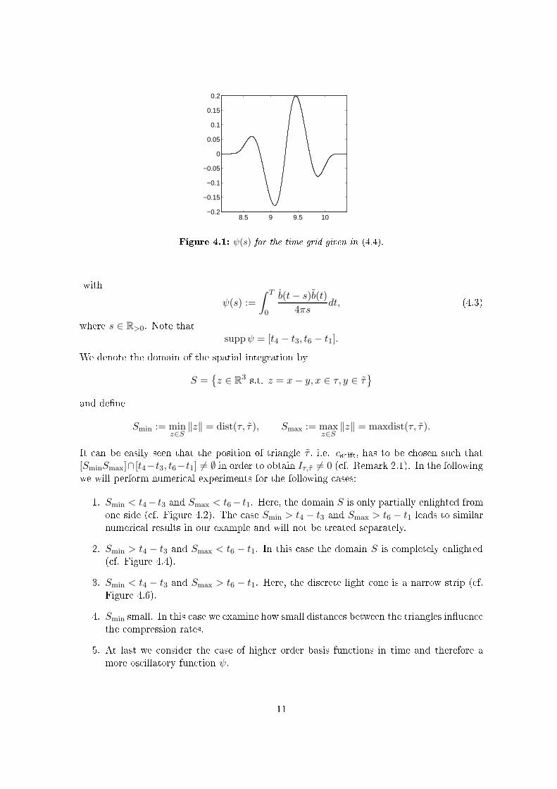
Figure 4.1: ψ(s) for the time grid given in (4.4).withψ(s) :=

∫ T

0

b(t− s)b(t)

4πsdt, (4.3)where s ∈ R>0. Note that

suppψ = [t4 − t3, t6 − t1].We denote the domain of the spatial integration byS =

z ∈ R

3 s.t. z = x− y, x ∈ τ, y ∈ τand dene

Smin := minz∈S

‖z‖ = dist(τ, τ ), Smax := maxz∈S

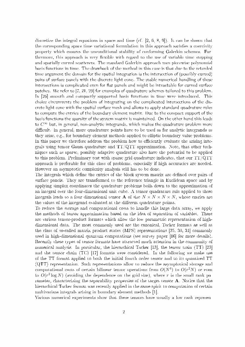
‖z‖ = maxdist(τ, τ ).It an be easily seen that the position of triangle τ , i.e. cshift, has to be hosen su h that[SminSmax]∩[t4−t3, t6−t1] 6= ∅ in order to obtain Iτ,τ 6= 0 ( f. Remark 2.1). In the followingwe will perform numeri al experiments for the following ases:1. Smin < t4− t3 and Smax < t6− t1. Here, the domain S is only partially enlighted fromone side ( f. Figure 4.2). The ase Smin > t4 − t3 and Smax > t6 − t1 leads to similarnumeri al results in our example and will not be treated separately.2. Smin > t4 − t3 and Smax < t6 − t1. In this ase the domain S is ompletely enlighted( f. Figure 4.4).3. Smin < t4 − t3 and Smax > t6 − t1. Here, the dis rete light one is a narrow strip ( f.Figure 4.6).4. Smin small. In this ase we examine how small distan es between the triangles inuen ethe ompression rates.5. At last we onsider the ase of higher order basis fun tions in time and therefore amore os illatory fun tion ψ. 11

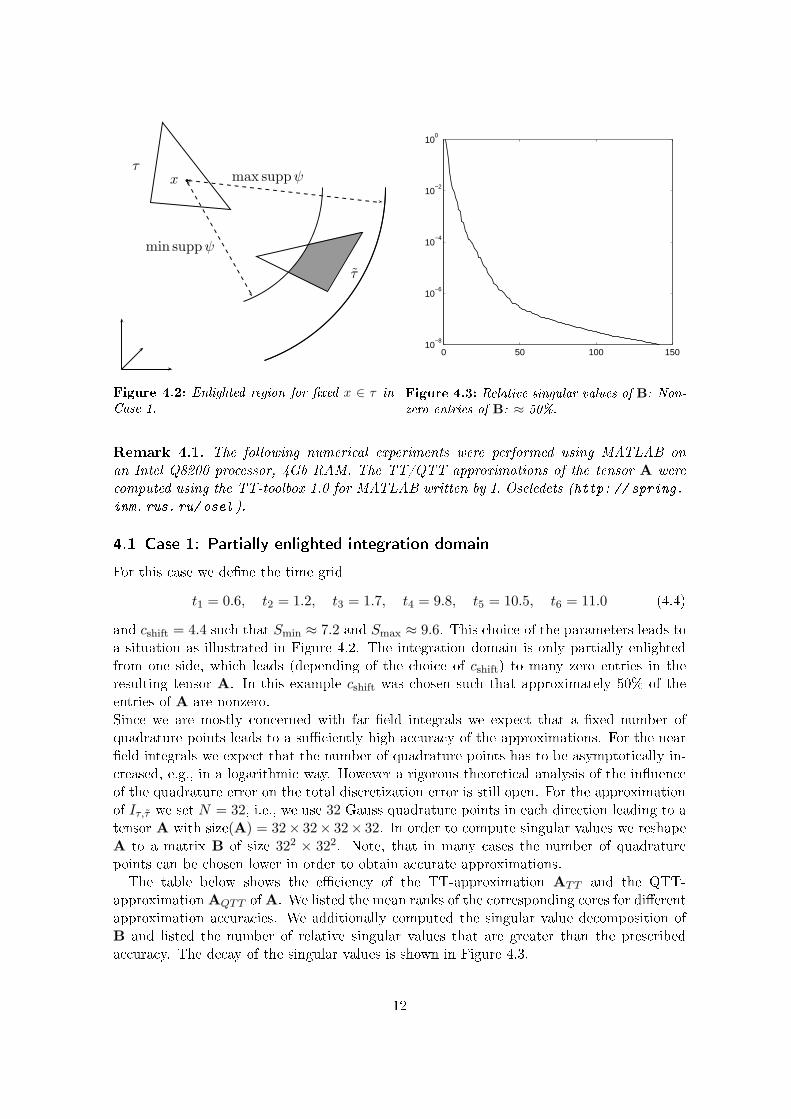
τx max suppψ

min suppψ

τ

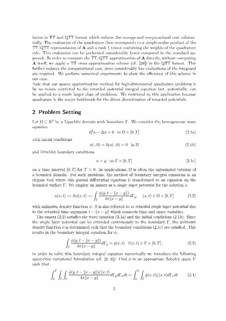
Figure 4.2: Enlighted region for xed x ∈ τ inCase 1. 0 50 100 15010

−8

10−6

10−4

10−2

100

Figure 4.3: Relative singular values of B: Non-zero entries of B: ≈ 50%.Remark 4.1. The following numeri al experiments were performed using MATLAB onan Intel Q8200 pro essor, 4Gb RAM. The TT/QTT approximations of the tensor A were omputed using the TT-toolbox 1.0 for MATLAB written by I. Oseledets (http: // spring.inm. rus. ru/ osel ).4.1 Case 1: Partially enlighted integration domainFor this ase we dene the time gridt1 = 0.6, t2 = 1.2, t3 = 1.7, t4 = 9.8, t5 = 10.5, t6 = 11.0 (4.4)and cshift = 4.4 su h that Smin ≈ 7.2 and Smax ≈ 9.6. This hoi e of the parameters leads toa situation as illustrated in Figure 4.2. The integration domain is only partially enlightedfrom one side, whi h leads (depending of the hoi e of cshift) to many zero entries in theresulting tensor A. In this example cshift was hosen su h that approximately 50% of theentries of A are nonzero.Sin e we are mostly on erned with far eld integrals we expe t that a xed number ofquadrature points leads to a su iently high a ura y of the approximations. For the neareld integrals we expe t that the number of quadrature points has to be asymptoti ally in- reased, e.g., in a logarithmi way. However a rigorous theoreti al analysis of the inuen eof the quadrature error on the total dis retization error is still open. For the approximationof Iτ,τ we set N = 32, i.e., we use 32 Gauss quadrature points in ea h dire tion leading to atensor A with size(A) = 32× 32× 32× 32. In order to ompute singular values we reshape

A to a matrix B of size 322 × 322. Note, that in many ases the number of quadraturepoints an be hosen lower in order to obtain a urate approximations.The table below shows the e ien y of the TT-approximation ATT and the QTT-approximation AQTT ofA. We listed the mean ranks of the orresponding ores for dierentapproximation a ura ies. We additionally omputed the singular value de omposition ofB and listed the number of relative singular values that are greater than the pres ribeda ura y. The de ay of the singular values is shown in Figure 4.3.12

A ura y Mean rank of ATT Mean rank of AQTT Rel. SV of B10−2 5.7 8.0 710−3 9.4 15.2 1210−4 13.0 23.1 1810−5 18.7 33.4 2810−6 25.4 45.5 41It an be observed that the ranks of the TT- and QTT-approximation are small, espe iallyfor low and medium a ura ies. The low ranks in this ase ould be found also for other ongurations of the numeri al experiment. In general it an be noti ed that the ompres-sion in this ase is better if many entries of A are zero or in other words that the enlightedpart of the integration domain is small. (That a sparse A however does not ne essarily leadto good ompression rates an be seen in Se tion 4.3).In the next table we ompare the time that is needed to ompute the approximations

QG, QTT and QQTT for dierent a ura ies of the TT- and QTT-approximation. We as-sume that A, ATT , and AQTT are given in ea h ase, so that only the dierent s alarprodu ts (3.2)-(3.4) have to be evaluated. Furthermore we ompute the relative errorsEG,TT and EG,QTT ( f. (3.5)) in order to see the ee t of the additional approximation onthe quadrature result.A ura y Time QG Time QTT EG,TT Time QQTT EG,QTT

10−2 100 1.3 2 · 10−3 9.8 2 · 10−4

10−3 100 1.3 4 · 10−5 10.1 1 · 10−4

10−4 100 1.4 2 · 10−6 10.3 6 · 10−6

10−5 100 1.5 1 · 10−7 10.8 2 · 10−7

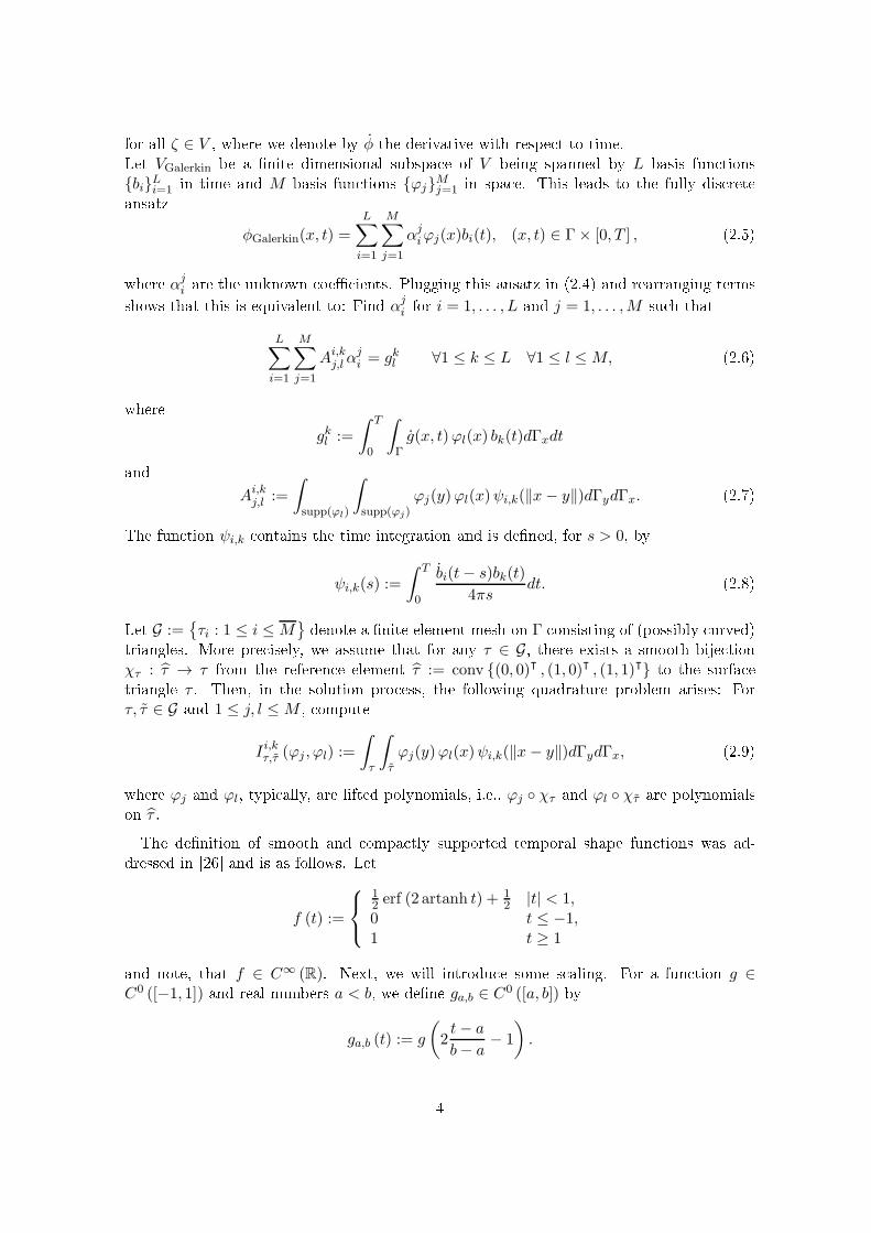
10−6 100 1.6 7 · 10−8 11.2 4 · 10−8It an be seen above that the evaluation of QTT and QQTT is onsiderably faster thanthe evaluation of QG due to the low ranks of ATT and AQTT and the indu ed low numberof arithmeti operations that are needed to ompute the orresponding s alar produ ts.Furthermore it an be observed that the errors EG,TT and EG,QTT are small even for lowand medium a ura ies of the TT- and QTT-approximation. In this ase it is su ientto determine ATT and AQTT with relatively low a ura y in order to obtain a urateapproximations for QG. On the one hand this is advantageous sin e we benet from lowranks in this ase and on the other hand the omputation of ATT and AQTT dire tly viaTT/QTT ross approximation be omes heaper as well ( f. Se tion 4.6).4.2 Case 2: Completely enlighted integration domainFor this ase we again use the time grid (4.4) and set cshift = 5.1 su h that Smin ≈ 8.42and Smax ≈ 10.28. We are therefore in the situation where the integration domain τ × τis ompletely enlighted ( f. Figure 4.4). Thus, A is in general densely populated with novanishing entries. We set again N = 32 and ompute the mean ranks of the TT- and QTTapproximation of A. The de ay of the relative singular values of the reshaped matrix B isshown in Figure 4.5.The results of the numeri al experiments indi ate that the ompression rates in this aseare very similar to Case 1. Thus a fully populated tensor A does not have a severe negative13

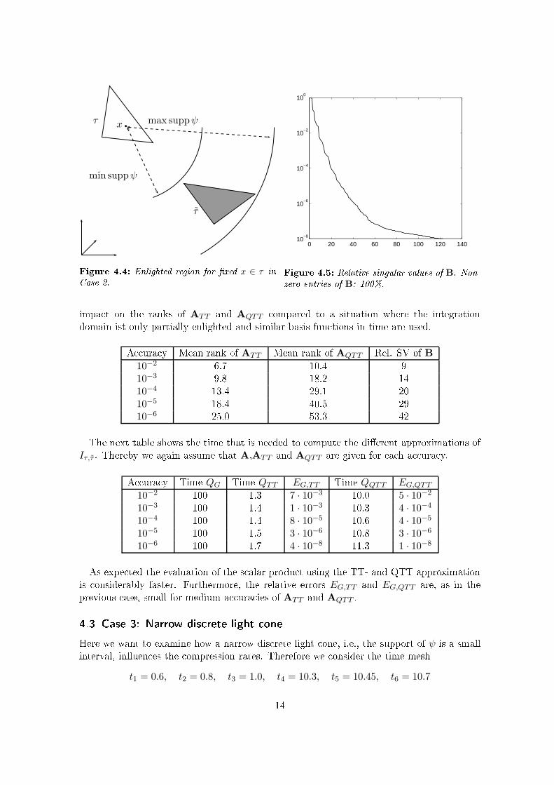
τ x max suppψ

min suppψ

τ

Figure 4.4: Enlighted region for xed x ∈ τ inCase 2. 0 20 40 60 80 100 120 14010

−8

10−6

10−4

10−2

100

Figure 4.5: Relative singular values of B. Non-zero entries of B: 100%.impa t on the ranks of ATT and AQTT ompared to a situation where the integrationdomain ist only partially enlighted and similar basis fun tions in time are used.A ura y Mean rank of ATT Mean rank of AQTT Rel. SV of B10−2 6.7 10.4 910−3 9.8 18.2 1410−4 13.4 29.1 2010−5 18.4 40.5 2910−6 25.0 53.3 42The next table shows the time that is needed to ompute the dierent approximations of

Iτ,τ . Thereby we again assume that A,ATT and AQTT are given for ea h a ura y.A ura y Time QG Time QTT EG,TT Time QQTT EG,QTT

10−2 100 1.3 7 · 10−3 10.0 5 · 10−2

10−3 100 1.4 1 · 10−3 10.3 4 · 10−4

10−4 100 1.4 8 · 10−5 10.6 4 · 10−5

10−5 100 1.5 3 · 10−6 10.8 3 · 10−6

10−6 100 1.7 4 · 10−8 11.3 1 · 10−8As expe ted the evaluation of the s alar produ t using the TT- and QTT approximationis onsiderably faster. Furthermore, the relative errors EG,TT and EG,QTT are, as in theprevious ase, small for medium a ura ies of ATT and AQTT .4.3 Case 3: Narrow dis rete light oneHere we want to examine how a narrow dis rete light one, i.e., the support of ψ is a smallinterval, inuen es the ompression rates. Therefore we onsider the time mesht1 = 0.6, t2 = 0.8, t3 = 1.0, t4 = 10.3, t5 = 10.45, t6 = 10.714

τ x max suppψ

min suppψ

τ

Figure 4.6: Enlighted region for xed x ∈ τ inCase 3. 0 50 100 150 200 250 30010

−8

10−6

10−4

10−2

100

Figure 4.7: Relative singular values of B. Non-zero entries of B: ≈ 64%.su h that suppψ = [9.3, 10.1]. Choosing cshift = 5.4 leads to the ase where Smin < 9.3 andSmax > 10.1. We are thus in the situation illustrated in Figure 4.6. We set again N = 32 and ompute the mean ranks of the TT- and QTT approximation of A whi h has approximately64% nonzero entries. The de ay of the relative singular values of the reshaped matrix B isshown in Figure 4.7.A ura y Mean rank of ATT Mean rank of AQTT Rel. SV of B

10−2 14.4 21.8 2310−3 23.3 46.8 3710−4 33.2 69.7 6010−5 44.3 97.1 8910−6 57.0 130.1 126As one an see in the table above, the ompression rates are worse than in the previous ases. This is not surprising sin e ψ has the same os illatory behavior as before but varieson a smaller interval. The approximation of the tensor A, whi h is based on the evaluationof ψ at dierent points in τ × τ and not only in a narrow strip ontaining the dis rete light one, is therefore learly more di ult. This is onrmed by various numeri al experiments.The narrower the dis rete light one is, the higher are the mean ranks of the TT- and QTTapproximation of A in general. This ase is therefore an example where a more sparse Adoes not lead to better ompression rates.Although the mean ranks of ATT and AQTT are larger here than in the previous ases,the ompression is still good enough to redu e the omputing times of the quadratures onsiderably.

15

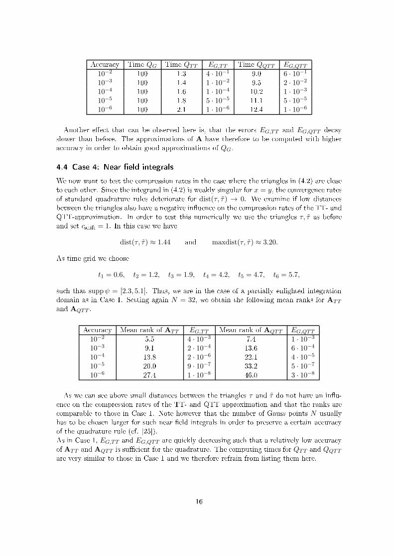
A ura y Time QG Time QTT EG,TT Time QQTT EG,QTT

10−2 100 1.3 4 · 10−1 9.0 6 · 10−1

10−3 100 1.4 1 · 10−2 9.5 2 · 10−2

10−4 100 1.6 1 · 10−4 10.2 1 · 10−3

10−5 100 1.8 5 · 10−5 11.1 5 · 10−5

10−6 100 2.1 1 · 10−6 12.4 1 · 10−6Another ee t that an be observed here is, that the errors EG,TT and EG,QTT de ayslower than before. The approximations of A have therefore to be omputed with highera ura y in order to obtain good approximations of QG.4.4 Case 4: Near eld integralsWe now want to test the ompression rates in the ase where the triangles in (4.2) are loseto ea h other. Sin e the integrand in (4.2) is weakly singular for x = y, the onvergen e ratesof standard quadrature rules deteriorate for dist(τ, τ ) → 0. We examine if low distan esbetween the triangles also have a negative inuen e on the ompression rates of the TT- andQTT-approximation. In order to test this numeri ally we use the triangles τ, τ as beforeand set cshift = 1. In this ase we havedist(τ, τ) ≈ 1.44 and maxdist(τ, τ ) ≈ 3.20.As time grid we hoose

t1 = 0.6, t2 = 1.2, t3 = 1.9, t4 = 4.2, t5 = 4.7, t6 = 5.7,su h that suppψ = [2.3, 5.1]. Thus, we are in the ase of a partially enlighted integrationdomain as in Case 1. Setting again N = 32, we obtain the following mean ranks for ATTand AQTT .A ura y Mean rank of ATT EG,TT Mean rank of AQTT EG,QTT

10−2 5.5 4 · 10−3 7.4 1 · 10−3

10−3 9.1 2 · 10−4 13.6 6 · 10−4

10−4 13.8 2 · 10−6 22.1 4 · 10−5

10−5 20.0 9 · 10−7 33.2 5 · 10−7

10−6 27.4 1 · 10−8 46.0 3 · 10−8As we an see above small distan es between the triangles τ and τ do not have an inu-en e on the ompression rates of the TT- and QTT approximation and that the ranks are omparable to those in Case 1. Note however that the number of Gauss points N usuallyhas to be hosen larger for su h near eld integrals in order to preserve a ertain a ura yof the quadrature rule ( f. [25).As in Case 1, EG,TT and EG,QTT are qui kly de reasing su h that a relatively low a ura yof ATT and AQTT is su ient for the quadrature. The omputing times for QTT and QQTTare very similar to those in Case 1 and we therefore refrain from listing them here.16

8.5 9 9.5 10−0.3

−0.2

−0.1

0

0.1

0.2

Figure 4.8: Plot of ψhigh,1. 8.5 9 9.5 10−0.4

−0.3

−0.2

−0.1

0

0.1

0.2

0.3

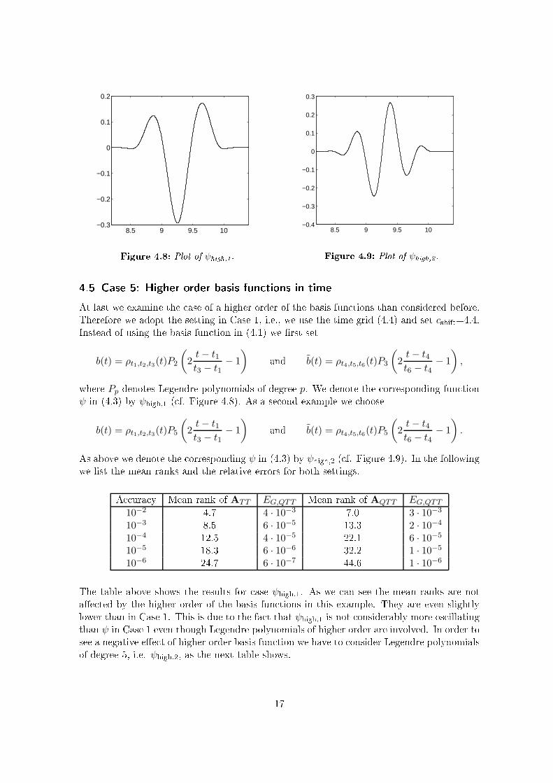
Figure 4.9: Plot of ψhigh,2.4.5 Case 5: Higher order basis fun tions in timeAt last we examine the ase of a higher order of the basis fun tions than onsidered before.Therefore we adopt the setting in Case 1, i.e., we use the time grid (4.4) and set cshift=4.4.Instead of using the basis fun tion in (4.1) we rst setb(t) = ρt1,t2,t3(t)P2

(2t− t1

t3 − t1− 1

) and b(t) = ρt4,t5,t6(t)P3

(2t− t4

t6 − t4− 1

),where Pp denotes Legendre polynomials of degree p. We denote the orresponding fun tion

ψ in (4.3) by ψhigh,1 ( f. Figure 4.8). As a se ond example we hooseb(t) = ρt1,t2,t3(t)P5

(2t− t1

t3 − t1− 1

) and b(t) = ρt4,t5,t6(t)P5

(2t− t4

t6 − t4− 1

).As above we denote the orresponding ψ in (4.3) by ψhigh,2 ( f. Figure 4.9). In the followingwe list the mean ranks and the relative errors for both settings.A ura y Mean rank of ATT EG,QTT Mean rank of AQTT EG,QTT

10−2 4.7 4 · 10−3 7.0 3 · 10−3

10−3 8.5 6 · 10−5 13.3 2 · 10−4

10−4 12.5 4 · 10−5 22.1 6 · 10−5

10−5 18.3 6 · 10−6 32.2 1 · 10−5

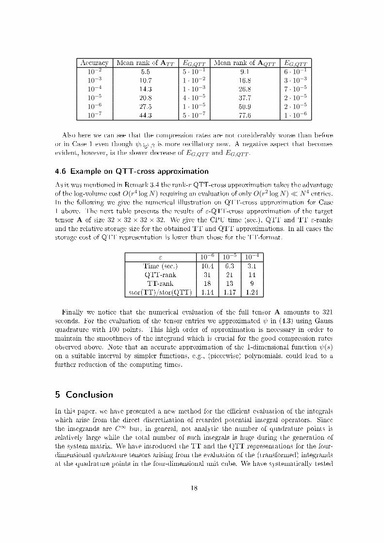
10−6 24.7 6 · 10−7 44.6 1 · 10−6The table above shows the results for ase ψhigh,1. As we an see the mean ranks are notae ted by the higher order of the basis fun tions in this example. They are even slightlylower than in Case 1. This is due to the fa t that ψhigh,1 is not onsiderably more os illatingthan ψ in Case 1 even though Legendre polynomials of higher order are involved. In order tosee a negative ee t of higher order basis fun tion we have to onsider Legendre polynomialsof degree 5, i.e. ψhigh,2, as the next table shows.17

A ura y Mean rank of ATT EG,QTT Mean rank of AQTT EG,QTT

10−2 5.5 5 · 10−1 9.1 6 · 10−1

10−3 10.7 1 · 10−2 16.8 3 · 10−3

10−4 14.3 1 · 10−3 26.8 7 · 10−5

10−5 20.8 4 · 10−5 37.7 2 · 10−5

10−6 27.5 1 · 10−5 50.9 2 · 10−5

10−7 44.3 5 · 10−7 77.6 1 · 10−6Also here we an see that the ompression rates are not onsiderably worse than beforeor in Case 1 even though ψhigh,2 is more os illatory now. A negative aspe t that be omesevident, however, is the slower de rease of EG,QTT and EG,QTT .4.6 Example on QTT- ross approximationAs it was mentioned in Remark 3.4 the rank-r QTT- ross approximation takes the advantageof the log-volume ost O(r4 logN) requiring an evaluation of only O(r2 logN) ≪ N4 entries.In the following we give the numeri al illustration on QTT- ross approximation for Case1 above. The next table presents the results of ε-QTT- ross approximation of the targettensor A of size 32 × 32 × 32 × 32. We give the CPU time (se .), QTT and TT ε-ranksand the relative storage size for the obtained TT and QTT approximations. In all ases thestorage ost of QTT representation is lower than those for the TT-format.ε 10−6 10−5 10−4Time (se .) 10.4 6.3 3.1QTT-rank 31 21 14TT-rank 18 13 9stor(TT)/stor(QTT) 1.14 1.17 1.24Finally we noti e that the numeri al evaluation of the full tensor A amounts to 321se onds. For the evaluation of the tensor entries we approximated ψ in (4.3) using Gaussquadrature with 100 points. This high order of approximation is ne essary in order tomaintain the smoothness of the integrand whi h is ru ial for the good ompression ratesobserved above. Note that an a urate approximation of the 1-dimensional fun tion ψ(s)on a suitable interval by simpler fun tions, e.g., (pie ewise) polynomials, ould lead to afurther redu tion of the omputing times.5 Con lusionIn this paper, we have presented a new method for the e ient evaluation of the integralswhi h arise from the dire t dis retization of retarded potential integral operators. Sin ethe integrands are C∞ but, in general, not analyti the number of quadrature points isrelatively large while the total number of su h integrals is huge during the generation ofthe system matrix. We have introdu ed the TT and the QTT representations for the four-dimensional quadrature tensors arising from the evaluation of the (transformed) integrandsat the quadrature points in the four-dimensional unit ube. We have systemati ally tested18

the sensitivity of the algorithm with respe t a) to dierent ases how the smeared dis retelight one interse ts the spatial mesh, b) to the distan e of the surfa e panels indu ingdierent nearly-singular behaviors of the integrands, and ) to the polynomial degree of thetemporal approximation. In all ases the ompression by the TT and QTT representationis impressive.Sin e both, the TT and the QTT formats require as input the full tensor it is important tosubstitute the orresponding full-to-TT and full-to-QTT approximation algorithms by theiradaptive ross versions. We have performed numeri al experiments whi h show that the ompression rates by the adaptive TT- ross and QTT- ross representations are omparablewith the original ones while the generation of the full tensor an be avoided.A knowledgement. The authors are thankful to Dr. I. Oseledets (INM RAS, Mos ow)for the assistan e with the QTT- ross-approximation MATLAB routine.Referen es[1 J. Ballani. Fast evaluation of singular BEM integrals based on tensor approximations.Preprint 77/2010, MPI MiS, Leipzig 2010.[2 A. Bamberger and T. Ha Duong. Formulation Variationnelle Espa e-Temps pur leCal ul par Potientiel Retardé de la Dira tion d'une Onde A oustique. Math. Meth.in the Appl. S i., 8:405435, 1986.[3 L. Banjai. Multistep and multistage onvolution quadrature for the wave equation:Algorithms and experiments. Preprint 58/2009, MPI Leipzig, a epted for publi ationin SISC.[4 L. Banjai and S. Sauter. Rapid solution of the wave equation in unbounded domains.SIAM Journal on Numeri al Analysis, 47:227249, 2008.[5 L. Banjai and M S hanz. Wave Propagation Problems treated with ConvolutionQuadrature and BEM. Preprint 60/2010, MPI Leipzig.[6 Y. Ding, A. Forestier, and T. Ha Duong. A Galerkin s heme for the time domain integralequation of a ousti s attering from a hard surfa e. The Journal of the A ousti alSo iety of Ameri a, 86(4):15661572, 1989.[7 J. El Gharib. Problèmes de potentiels rétardes pour l'a oustique. PhD thesis, É olePolyte hnique, 1999.[8 T. Ha-Duong. On retarded potential boundary integral equations and their dis reti-sation. In Topi s in Computational Wave Propagation: Dire t and Iverse Problems,volume 31 of Le t. Notes Comput. S i. Eng., pages 301336. Springer, Berlin, 2003.[9 T. Ha-Duong, B. Ludwig, and I. Terrasse. A Galerkin BEM for transient a ousti s attering by an absorbing obsta le. International Journal for Numeri al Methods inEngineering, 57:18451882, 2003.[10 W. Ha kbus h, B.N. Khoromskij, S. Sauter, and E. Tyrtyshnikov. Use of Tensor For-mats in Ellipti Eigenvalue Problems. Preprint 78, MPI MiS, Leipzig 2008. Numer.Lin. Alg. Appl., 2011, DOI: 10.1002/nla.793.19

[11 W. Ha kbus h, W. Kress, and S. Sauter. Sparse onvolution quadrature for time domainboundary integral formulations of the wave equation by uto and panel- lustering.In M. S hanz and O. Steinba h, editors, Boundary Element Analysis, pages 113134.Springer, 2007.[12 W. Ha kbus h, W. Kress, and S. Sauter. Sparse onvolution quadrature for time domainboundary integral formulations of the wave equation. IMA, J. Numer. Anal., 29:158179, 2009.[13 W. Ha kbus h and S. Kühn. A new s heme for the tensor representation. J. of Fourieranalysis and appli ations, 15:706722, 2009.[14 S. Holtz, T. Rohwedder, and R. S hneider. On manifold of tensors of xed TT-rank.Te hni al Report 61, TU Berlin, 2010.[15 B.N. Khoromskij. Introdu tion to Tensor Numeri al Methods in S ienti Computing.Le ture Notes, University/ETH Züri h, Preprint 06-2011, Universität Züri h 2011, pp.1-238.[16 B.N. Khoromskij. Tensors-stru tured Numeri al Methods in S ienti Computing: Sur-vey on Re ent Advan es. Preprint 21/2010, MPI MIS Leipzig 2010 (submitted).[17 B.N. Khoromskij. O(d logN)-Quanti s Approximation of N -d Tensors in High-Dimensional Numeri al Modeling. Constru tive Approximation, pages 124, 2011. DOI:10.1007/s00365-011-9131-1. Preprint 55/2009 MPI MIS, Leipzig 2009.[18 B.N. Khoromskij, V. Khoromskaia, and H.-J. Flad. Numeri al Solution of the Hartree-Fo k Equation in Multilevel Tensor-stru tured Format. SIAM J. on S i. Comp.,33(1):4565, 2011.[19 B.N. Khoromskij and I. Oseledets. Quanti s-TT approximation of ellipti solutionoperators in higher dimensions. Preprint MPI MIS 79/2009, Leipzig 2009. To appearin Rus. J. of Numeri al Math., 2010.[20 T.G. Kolda and B.W. Bader. Tensor de ompositions and appli ations. SIAM Review,51/3:455500, 2009.[21 J.C. Nédéle , T. Abboud, and J. Volakis. Stable solution of the retarded potentialequations, Applied Computational Ele tromagneti s So iety (ACES) Symposium Di-gest, 17th Annual Review of Progress, Monterey, 2001.[22 I.V. Oseledets. Approximation of 2d × 2d matri es using tensor de omposition. SIAMJ. Matrix Anal. Appl., 31(4):21302145, 2010.[23 I.V. Oseledets and E.E. Tyrtyshnikov. Breaking the Curse of Dimensionality, or Howto Use SVD in Many Dimensions. SIAM J. S i. Comp., 31:37443759, 2009.[24 I.V. Oseledets and E.E. Tyrtyshnikov. TT- ross approximation for multidimensionalarrays. Lin. Alg. and its Appli ations, 432:7088, 2010.[25 S. Sauter and C. S hwab. Boundary Element Methods. Springer, Heidelberg, 2010.20

[26 S. Sauter and A. Veit. Adaptive Time Dis retization for Retarded Potentials. Preprint04-2011, Universität Züri h.[27 S. Sauter and A. Veit. Expli it Solutions of Retarded Boundary Integral Equations.Preprint 03-2011, Universität Züri h.[28 S. A. Sauter. Über die eziente Verwendung des Galerkinverfahrens zur Lösung Fred-holms her Integralglei hungen. PhD thesis, Inst. f. Prakt. Math., Universität Kiel,1992.[29 EP. Stephan, M. Mais hak, and E. Ostermann. Transient boundary element methodand numeri al evaluation of retarded potentials. In Computational S ien e - ICCS2008, pages 321330. Springer (5102), 2008.[30 G. Vidal. E ient lassi al simulation of slightly entangled quantum omputations.Phys. Rev. Lett., 91(14):1479021 1479024, 2003.[31 H. Wang and M. Thoss. Multilayer formulation of the multi onguration time-dependent Hartree theory. J. Chem. Phys., 119:12891299, 2003.[32 D. S. Weile, G. Pisharody, N. W. Chen, B. Shanker, and E. Mi hielssen. A novels heme for the solution of the time-domain integral equations of ele tromagneti s. IEEETransa tions on Antennas and Propagation, 52:283295, 2004.[33 D.S. Weile, A.A. Ergin, B. Shanker, and E. Mi hielssen. An a urate dis retizations heme for the numeri al solution of time domain integral equations. IEEE Antennasand Propagation So iety International Symposium, 2:741744, 2000.[34 D.S. Weile, B. Shanker, and E. Mi hielssen. An a urate s heme for the numeri al solu-tion of the time domain ele tri eld integral equation. IEEE Antennas and PropagationSo iety International Symposium, 4:516519, 2001.[35 S.R. White. Density-matrix algorithms for quantum renormalization groups. Phys.Rev. B, 48(14):1034510356, 1993.[36 A. Wildman, G. Pisharody, D. S. Weile, S. Balasubramaniam, and E. Mi hielssen. Ana urate s heme for the solution of the time-domain integral equations of ele tromagnet-i s using higher order ve tor bases and bandlimited extrapolation. IEEE Transa tionson Antennas and Propagation, 52:29732984, 2004.

21