Software Automation

L. Ridgway Scott

Fall 2009

1

1 Systems (r)evolution

Traditional systems research was based in three areas.

Operating

Databases

CompilersLanguages &Programming

Systems

Figure 1: Traditional areas of systems research

2

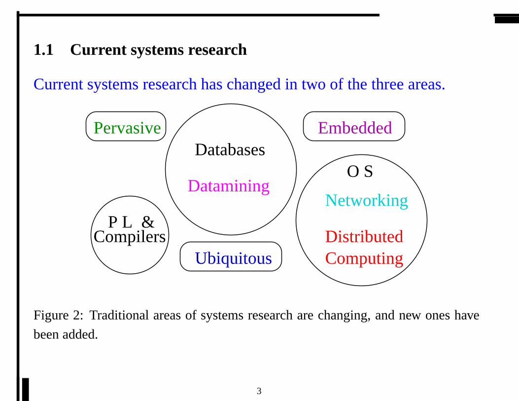
1.1 Current systems research

Current systems research has changed in two of the three areas.

Datamining

P L &Compilers

O S

DistributedComputing

Networking

DatabasesEmbedded

Ubiquitous

Pervasive

Figure 2: Traditional areas of systems research are changing, and new ones have

been added.

3

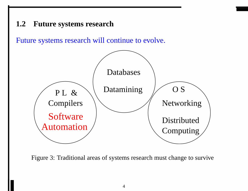
1.2 Future systems research

Future systems research will continue to evolve.

Automation

O S

DistributedComputing

Networking

DataminingP L &Compilers

Databases

Software

Figure 3: Traditional areas of systems research must changeto survive

4

New paradigms for softwaredevelopment

Hierarchical code development

Improves upon standard two level model: language+compiler

Allows appropriate optimizations to be done at different levels

Improves code correctness and decreases cost of code development

Automation of code production

Utilizes abstract descriptions as basis to generate code automatically

Leverages intrinsic domain languages

Improves code correctness and decreases cost of code development

Allows true optimization of generated code

5

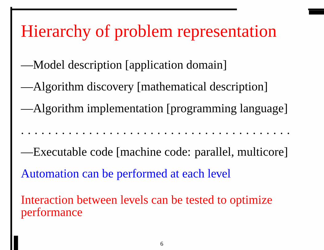
Hierarchy of problem representation

—Model description [application domain]

—Algorithm discovery [mathematical description]

—Algorithm implementation [programming language]

. . . . . . . . . . . . . . . . . . . . . . . . . . . . . . . . . . . . . . . .

—Executable code [machine code: parallel, multicore]

Automation can be performed at each level

Interaction between levels can be tested to optimizeperformance

6

Example of hierarchy: signalprocessing (Spiral project)

—Model description [Discrete Fourier Transform: DFT]

—Algorithm discovery [Cooley-Tukey FFT]

—Algorithm implementation [FFTW]

—Executable code [BLAS, ATLAS, OSKI]

Automation can be performed at each level: can derive

FFT from abstract definition of DFT

No need to hand-code for specific architectures

7

Paradigm limitations?

Must have hierarchical structure

But what doesn’t?

Common in computer architecture, compiler design, scientificcomputing, etc.

Automatic generation requires abstract model

In principle, this can be developed in any area, e.g., operatingsystems

Found in VLSI design, compiler design [3, 2], scientific computing[8, 7, 6, 5], etc.

8

Why focus on scientific computation?

Has built-in hierarchical structure

Models often built from simpler models

Laplace =⇒ Stokes=⇒ Navier-Stokes=⇒ Grade-2 fluids

Has built-in abstract descriptions

Equations are the language of science and engineering

E = mc2

F = ma

−ν ∆u + curl(u − α ∆u) × u + ∇ p = f

9

The software challenge

(Correct) interpretation of problem discription

Have to translate from a high-level description to low-level

executable, correctly!

Optimization of generated code

Have to solve disparate optimization problems at compile time or in

conjunction with run-time indicators

Tension between expressiveness and efficiencyIdeally the naive user could code in a high-level specificationlanguage and have it translated into efficient machine code.

10

Problem with single-language approach

C� � � � � � � � � � � � � � � � � �� � � � � � � � � � � � � � � � � �� � � � � � � � � � � � � � � � � �� � � � � � � � � � � � � � � � � �� � � � � � � � � � � � � � � � � �� � � � � � � � � � � � � � � � � �� � � � � � � � � � � � � � � � � �� � � � � � � � � � � � � � � � � �� � � � � � � � � � � � � � � � � �� � � � � � � � � � � � � � � � � �� � � � � � � � � � � � � � � � � �� � � � � � � � � � � � � � � � � �� � � � � � � � � � � � � � � � � �� � � � � � � � � � � � � � � � � �� � � � � � � � � � � � � � � � � �� � � � � � � � � � � � � � � � � �� � � � � � � � � � � � � � � � � �� � � � � � � � � � � � � � � � � �� � � � � � � � � � � � � � � � � �� � � � � � � � � � � � � � � � � �� � � � � � � � � � � � � � � � � �� � � � � � � � � � � � � � � � � �� � � � � � � � � � � � � � � � � �� � � � � � � � � � � � � � � � � �� � � � � � � � � � � � � � � � � �� � � � � � � � � � � � � � � � � �� � � � � � � � � � � � � � � � � �� � � � � � � � � � � � � � � � � �

� � � � � � � � � � � � � � � � � �� � � � � � � � � � � � � � � � � �� � � � � � � � � � � � � � � � � �� � � � � � � � � � � � � � � � � �� � � � � � � � � � � � � � � � � �� � � � � � � � � � � � � � � � � �� � � � � � � � � � � � � � � � � �� � � � � � � � � � � � � � � � � �� � � � � � � � � � � � � � � � � �� � � � � � � � � � � � � � � � � �� � � � � � � � � � � � � � � � � �� � � � � � � � � � � � � � � � � �� � � � � � � � � � � � � � � � � �� � � � � � � � � � � � � � � � � �� � � � � � � � � � � � � � � � � �� � � � � � � � � � � � � � � � � �� � � � � � � � � � � � � � � � � �� � � � � � � � � � � � � � � � � �� � � � � � � � � � � � � � � � � �� � � � � � � � � � � � � � � � � �� � � � � � � � � � � � � � � � � �� � � � � � � � � � � � � � � � � �� � � � � � � � � � � � � � � � � �� � � � � � � � � � � � � � � � � �� � � � � � � � � � � � � � � � � �� � � � � � � � � � � � � � � � � �� � � � � � � � � � � � � � � � � �� � � � � � � � � � � � � � � � � �

EX

PR

ES

SIV

EN

ES

S

EFFICIENCY

Scheme ML

C++

Fortran

Figure 4: The conflict between efficiency and expressiveness[M. Dragichescu].

11

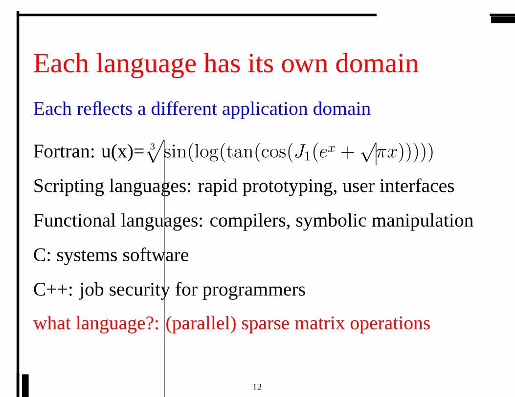
Each language has its own domain

Each reflects a different application domain

Fortran: u(x)=3√

sin(log(tan(cos(J1(ex +√

πx)))))

Scripting languages: rapid prototyping, user interfaces

Functional languages: compilers, symbolic manipulation

C: systems software

C++: job security for programmers

what language?: (parallel) sparse matrix operations

12

Nature of ‘answer’ changes over timeIn antiquity, an answer was a number: the length of the

diagonal of a unit square is√

2.

Later geometric figures were answers: elliptical orbits of

planets.

More recently, functions became an acceptable answer:

an ODE is solved by a Bessel function,J1.

In computational science, awell posed boundary value

problemis an acceptable answer.

All of these are abstractions that provide information ondemand.

13

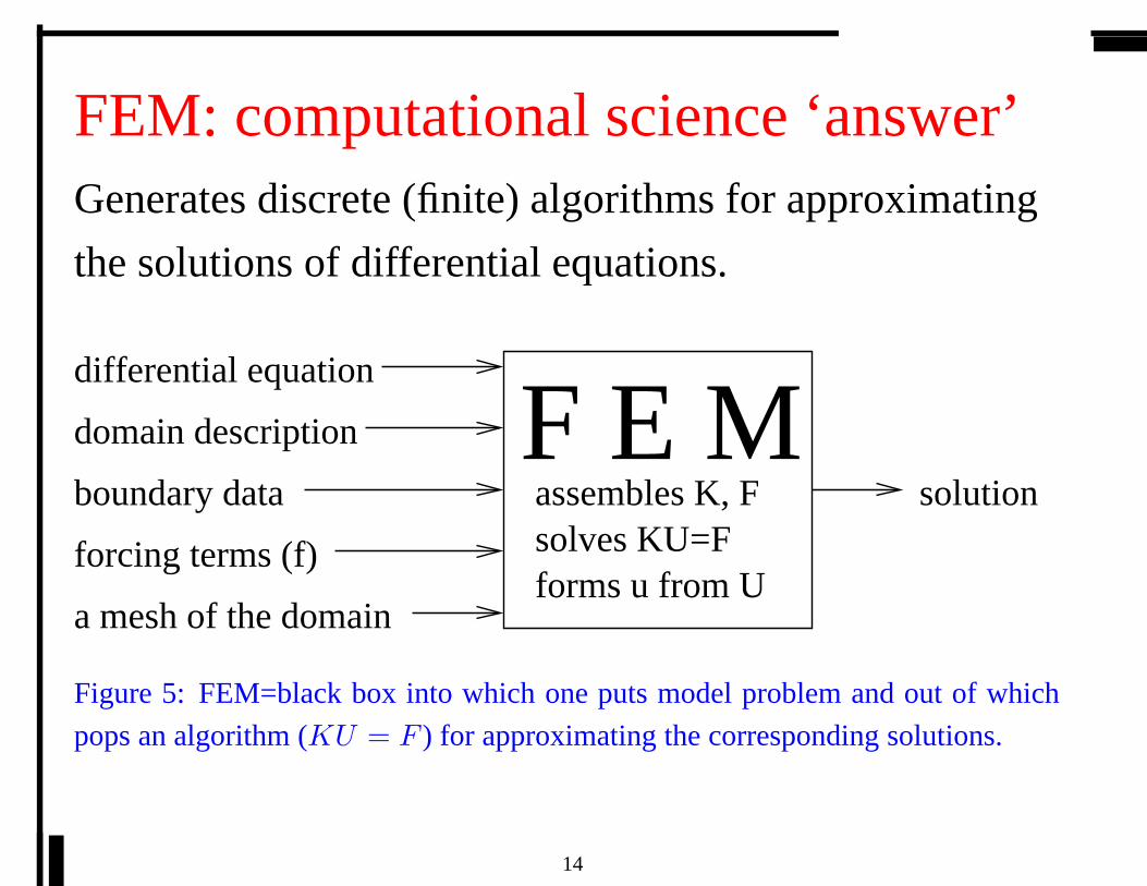
FEM: computational science ‘answer’Generates discrete (finite) algorithms for approximating

the solutions of differential equations.

solution

differential equation

domain description

boundary data

forcing terms (f)

a mesh of the domain

F E Massembles K, Fsolves KU=Fforms u from U

Figure 5: FEM=black box into which one puts model problem andout of which

pops an algorithm (KU = F ) for approximating the corresponding solutions.

14

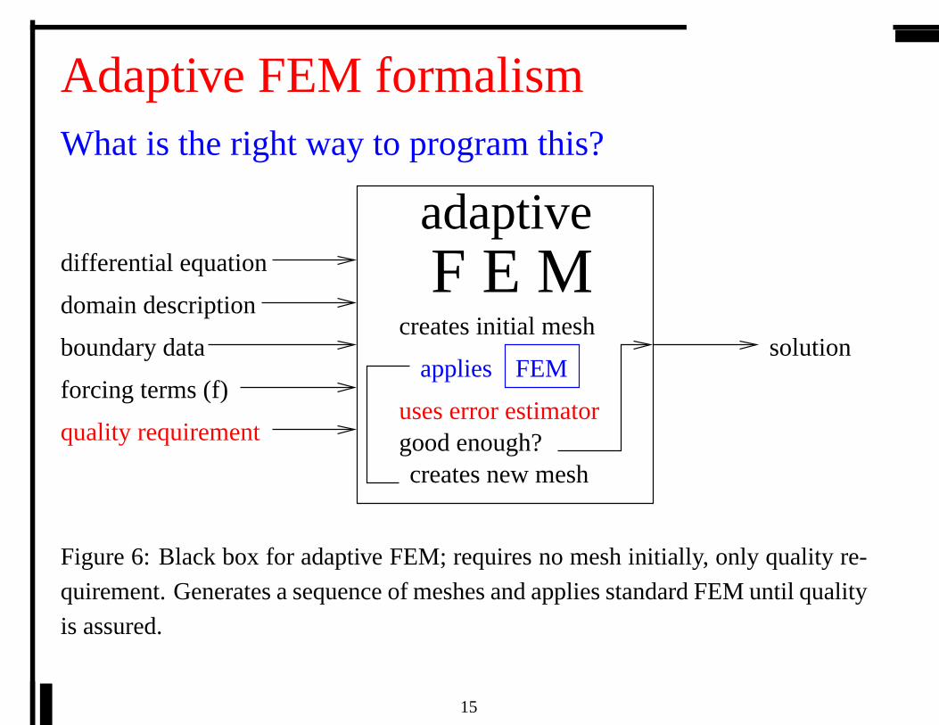
Adaptive FEM formalismWhat is the right way to program this?

FEM

quality requirement

differential equation

domain description

boundary data

forcing terms (f)

good enough?

solution

uses error estimator

adaptiveF E M

creates initial mesh

creates new mesh

applies

Figure 6: Black box for adaptive FEM; requires no mesh initially, only quality re-

quirement. Generates a sequence of meshes and applies standard FEM until quality

is assured.

15

Causes of efficiency–expressivenessconflict

Compilers perform transformations, not optimization.

Optimization at compile time, even if based on realistic performancemodels, would be wildly expensive (NPNP )

True optimization would have to involve evaluatingperformance.

Actual performance is often data dependent.

Best transformations are often domain dependent.

16

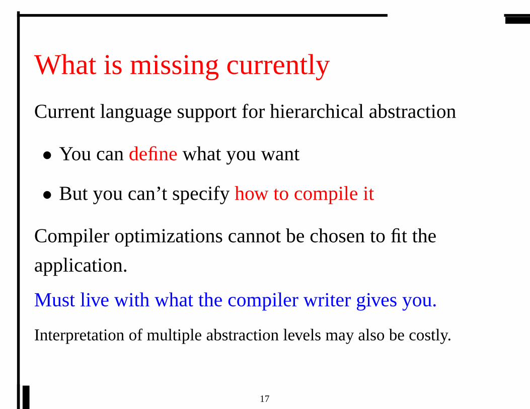
What is missing currently

Current language support for hierarchical abstraction

• You candefinewhat you want

• But you can’t specifyhow to compile it

Compiler optimizations cannot be chosen to fit the

application.

Must live with what the compiler writer gives you.

Interpretation of multiple abstraction levels may also be costly.

17

One solution: multi-lingual

approach

EX

PR

ES

SIV

EN

ES

S

EFFICIENCY

Scheme ML

C++

FortranC

Analysa

Figure 7: One way to combine efficiency and expressiveness [1].

18

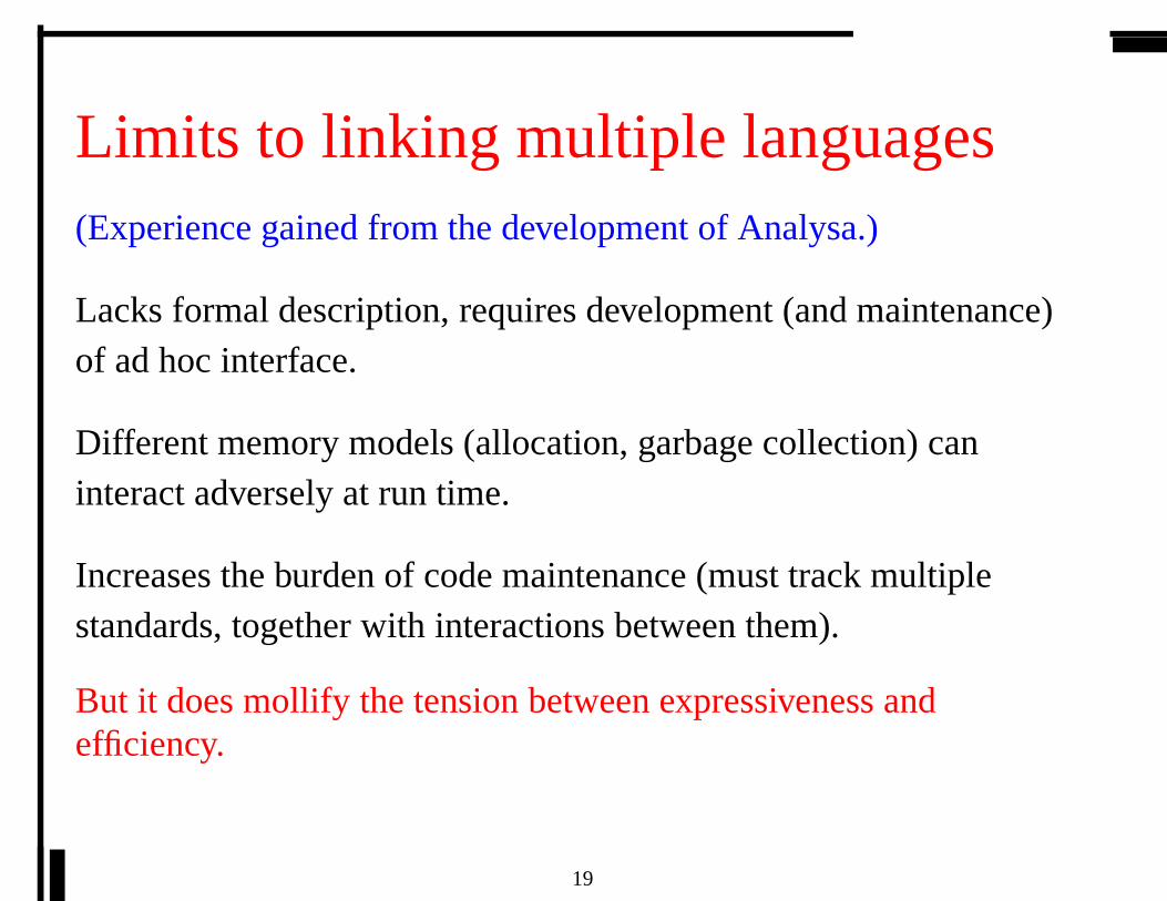
Limits to linking multiple languages(Experience gained from the development of Analysa.)

Lacks formal description, requires development (and maintenance)of ad hoc interface.

Different memory models (allocation, garbage collection)caninteract adversely at run time.

Increases the burden of code maintenance (must track multiplestandards, together with interactions between them).

But it does mollify the tension between expressiveness andefficiency.

19

Ken Kennedy’s telescoping languages

Languages

EX

PR

ES

SIV

EN

ES

S

EFFICIENCY

Scheme ML

C++

FortranC

Telescoping

Figure 8: Telescoping language approach [4].

20

Similar challengesfrom which we can learn

Same as problems in language/compiler design

Need to perform optimization and code generation

Often need to utilize these in an application-specific way (Spiral).

Hierarchical issues addressed in programming language

Manticore project for parallel computation

Algegra of code optimizations

Common to use Lambda Calculus or algebra of real numbers

Finite elements introduces optimization in vector spaces

21

2 Solving PDE’s: the FEM

Optimization of code for solving differential equations has beenstudied widely [5, 6, 7, 8].

Many of these approaches have been based on the finite elementmethod (FEM).

There are four distinct areas of finite element codes: function spaces,domain geometry/mesh, differential equation, and equation solution.

These are not hierarchical: interactions are multi-faceted.

Each area has it own natural language and its own optimizations.

But interactions require inter-procedural analysis toobtain ideal performance.

22

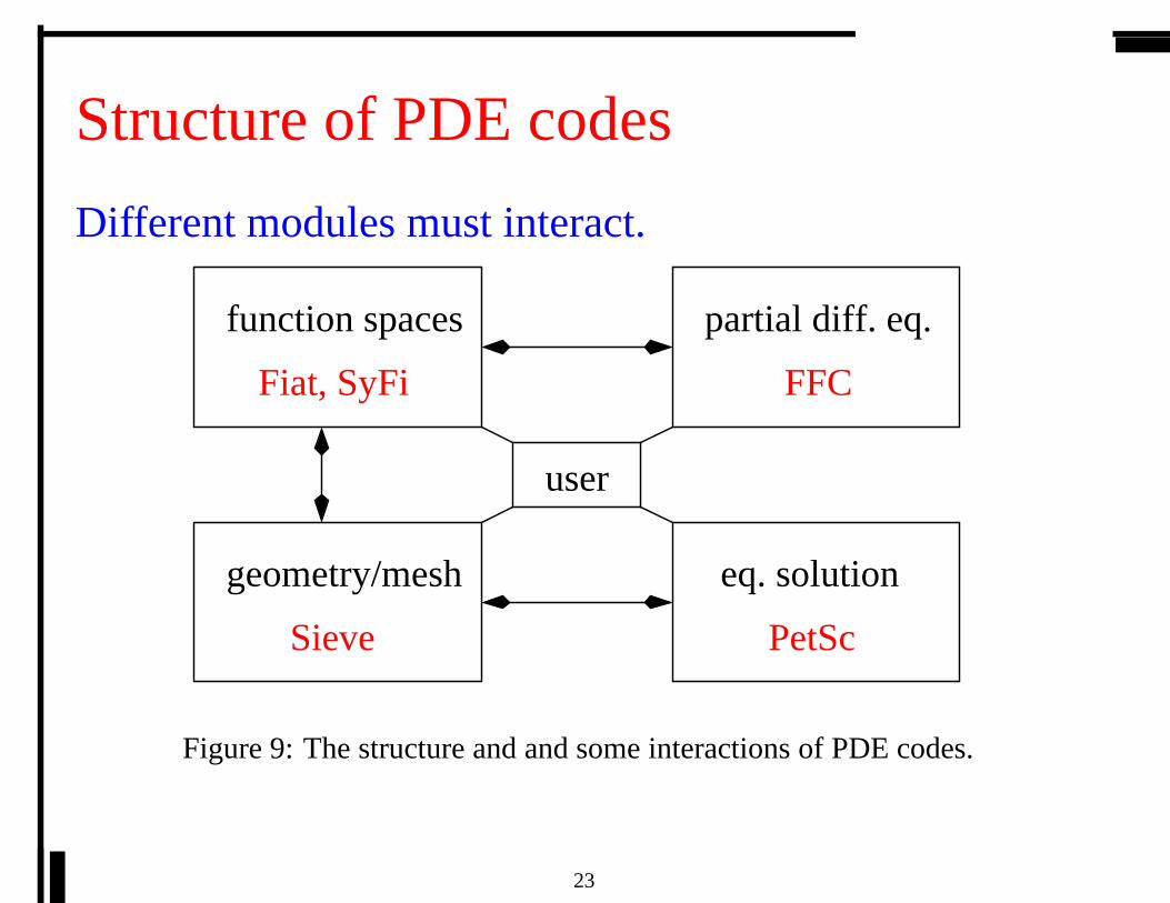
Structure of PDE codes

Different modules must interact.

user

function spaces

geometry/mesh eq. solution

partial diff. eq.

Fiat, SyFi

Sieve

FFC

PetSc

Figure 9: The structure and and some interactions of PDE codes.

23

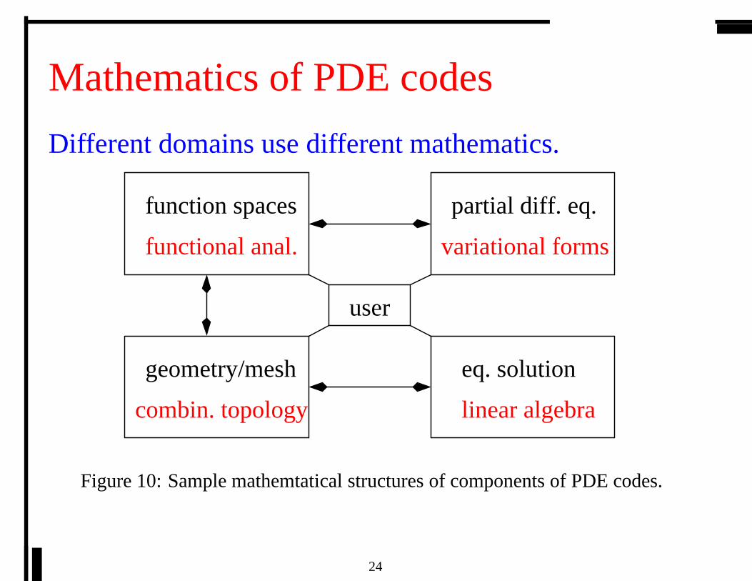
Mathematics of PDE codes

Different domains use different mathematics.

combin. topology

function spaces

geometry/mesh eq. solution

partial diff. eq.

user

variational forms

linear algebra

functional anal.

Figure 10: Sample mathemtatical structures of components of PDE codes.

24

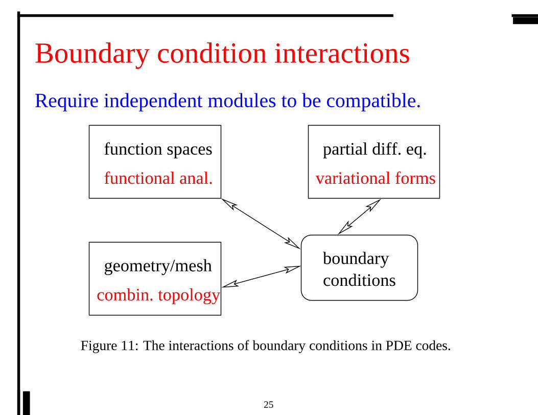
Boundary condition interactions

Require independent modules to be compatible.

boundary

function spaces

geometry/mesh

partial diff. eq.

variational formsfunctional anal.

combin. topologyconditions

Figure 11: The interactions of boundary conditions in PDE codes.

25

FErari interactions

FErari can be used as a matrix-free method.

May be of interest for multi-core processors.

FErari as a

function spaces

eq. solution

partial diff. eq.

variational forms

linear algebra

functional anal.

method

matrix−free

Figure 12: The interactions required to use FErari in PDE codes.

26

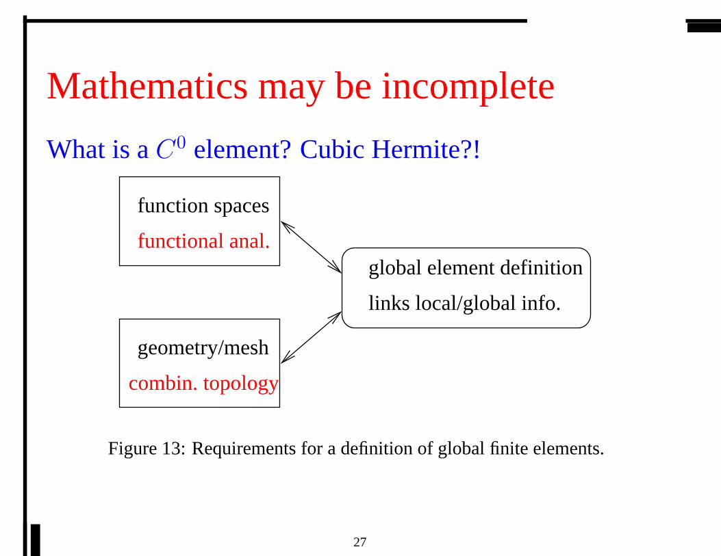
Mathematics may be incomplete

What is aC0 element? Cubic Hermite?!

global element definition

function spaces

geometry/mesh

functional anal.

combin. topology

links local/global info.

Figure 13: Requirements for a definition of global finite elements.

27

Software automation paradigm

application domain correct translation

code optimizationmath. abstraction

Figure 14: Components of the software automation paradigm.

Current (functional) PL research fits this paradigm:

Lambda calculus

application domain

math. abstraction

language compiler

Figure 15: PL paradigm as software automation.

28

Is Software Automation CS?Is it Math?Many areas now claim to be bothAlgorithms and complexity

Combinatorics

Computational biology

Software Automation is clearly

Computational Mathematics

29

FFC examples

# Copyright (c) 2005 Johan Jansson.

# Licensed under the GNU GPL Version 2

#

# The bilinear form e(u) : e(u) for linear

# elasticity with e(u) = grad(u) + grad(u)ˆT

#

# Compile this form with FFC: ffc Elasticity.form

element = FiniteElement("Vector Lagrange", "tetrahedron ", 1)

v = BasisFunction(element)

u = BasisFunction(element)

a = (u[i].dx(j) + u[j].dx(i)) * (v[i].dx(j) + v[j].dx(i)) * d x

30

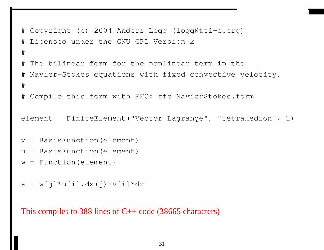
# Copyright (c) 2004 Anders Logg (logg@tti-c.org)

# Licensed under the GNU GPL Version 2

#

# The bilinear form for the nonlinear term in the

# Navier-Stokes equations with fixed convective velocity.

#

# Compile this form with FFC: ffc NavierStokes.form

element = FiniteElement("Vector Lagrange", "tetrahedron ", 1)

v = BasisFunction(element)

u = BasisFunction(element)

w = Function(element)

a = w[j]*u[i].dx(j)*v[i]*dx

This compiles to 388 lines of C++ code (38665 characters)

31

3 Code generation example: matrix formation

Formation of matrices takes substantialtime in finite element computations.

Disadvantage of finite elements over finite differences.

But standard algorithm can be far from optimal.

A general formalism can be automated called FErari:

Finite Element ReArRangement of Integrals

Eliminates efficiency penalty of finite elements.

32

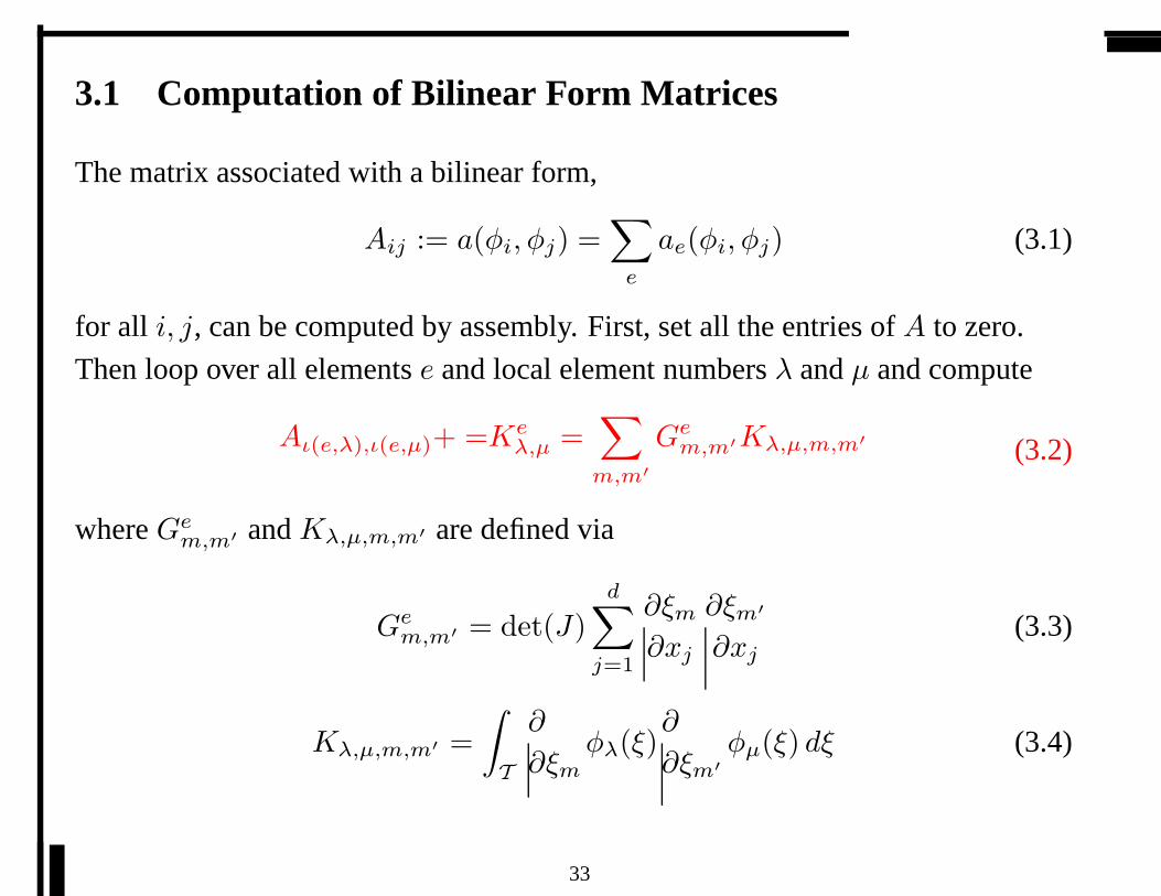
3.1 Computation of Bilinear Form Matrices

The matrix associated with a bilinear form,

Aij := a(φi, φj) =∑

e

ae(φi, φj) (3.1)

for all i, j, can be computed by assembly. First, set all the entries ofA to zero.

Then loop over all elementse and local element numbersλ andµ and compute

Aι(e,λ),ι(e,µ)+ =Keλ,µ =

∑

m,m′

Gem,m′Kλ,µ,m,m′ (3.2)

whereGem,m′ andKλ,µ,m,m′ are defined via

Gem,m′ = det(J)

d∑

j=1

∂ξm

∂xj

∂ξm′

∂xj

(3.3)

Kλ,µ,m,m′ =

∫

T

∂

∂ξm

φλ(ξ)∂

∂ξm′

φµ(ξ) dξ (3.4)

33

3.2 Matrix computation strategy

We optimize the computation of each

Keλ,µ =

∑

m,m′

Gem,m′Kλ,µ,m,m′ (3.5)

whereGem,m′ = det(J)

dX

j=1

∂ξm

∂xj

∂ξm′

∂xj

Kλ,µ,m,m′ =

Z

T

∂

∂ξm

φλ(ξ)∂

∂ξm′

φµ(ξ) dξ

Collection of dot products of fixed vectors (K) with

varying set of vectors (G’s encode “geometry”

information of elements).

Pre-computations can be done, based on relations amongtheK ’s, that reduce computational effort substantially.

34

3.3 TensorK for quadratics

zero entries,trivial entriesandcolinear entries(−4K3,1 = K3,4 = K4,1)

3 0 0 -1 1 1 -4 -4 0 4 0 0

0 0 0 0 0 0 0 0 0 0 0 0

0 0 0 0 0 0 0 0 0 0 0 0

-1 0 0 3 1 1 0 0 4 0 -4 -4

1 0 0 1 3 3 -4 0 0 0 0 -4

1 0 0 1 3 3 -4 0 0 0 0 -4

-4 0 0 0 -4 -4 8 4 0 -4 0 4

-4 0 0 0 0 0 4 8 -4 -8 4 0

0 0 0 4 0 0 0 -4 8 4 -8 -4

4 0 0 0 0 0 -4 -8 4 8 -4 0

0 0 0 -4 0 0 0 4 -8 -4 8 4

0 0 0 -4 -4 -4 4 0 -4 0 4 8

35

3.4 ComputingK for quadratics

Taking advantage of these simplifications, eachKe for quadratics intwo dimensions can be computed with at most 18 floating pointoperations instead of 288 floating point operations: animprovementof a factor of sixteen in computational complexity.

On the other hand, there are only 64 nonzero entries in eachK. Soeliminating multiplications by zero gives a four fold improvement.

Sparse matrix accumulation requires at least 76 (=36+36+4)memory references, not including sparse matrix indexing. Even ifthe matrix is stored in symmetric form, at least 46 (=21+21+4)memory references are needed.

Computational complexity can be

less than cost of memory references.

36

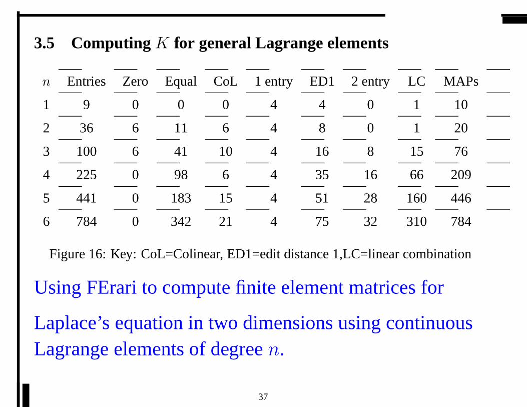
3.5 ComputingK for general Lagrange elements

n Entries Zero Equal CoL 1 entry ED1 2 entry LC MAPs

1 9 0 0 0 4 4 0 1 10

2 36 6 11 6 4 8 0 1 20

3 100 6 41 10 4 16 8 15 76

4 225 0 98 6 4 35 16 66 209

5 441 0 183 15 4 51 28 160 446

6 784 0 342 21 4 75 32 310 784

Figure 16: Key: CoL=Colinear, ED1=edit distance 1,LC=linear combination

Using FErari to compute finite element matrices for

Laplace’s equation in two dimensions using continuousLagrange elements of degreen.

37

from Numeric import zeros

G=zeros(4,"d")

def K(K,jinv):

detinv = 1.0/(jinv[0,0]*jinv[1,1] - jinv[0,1]*jinv[1,0] )

G[0] = ( jinv[0,0]**2 + jinv[1,0]**2 ) * detinv

G[1] = ( jinv[0,0]*jinv[0,1]+jinv[1,0]*jinv[1,1] ) * deti nv

G[2] = G[1]

G[3] = ( jinv[0,1]**2 + jinv[1,1]**2 ) * detinv

K[1,1] = 0.5 * G[0]

K[1,0] = -0.5 * G[1]- K[1,1]

K[2,1] = 0.5 * G[2]

K[2,0] = -0.5 * G[3]- K[2,1]

K[0,0] = -1.0 * K[1,0] + -1.0 * K[2,0]

K[2,2] = 0.5 * G[3]

K[0,1] = K[1,0]

K[0,2] = K[2,0]

K[1,2] = K[2,1]

return K

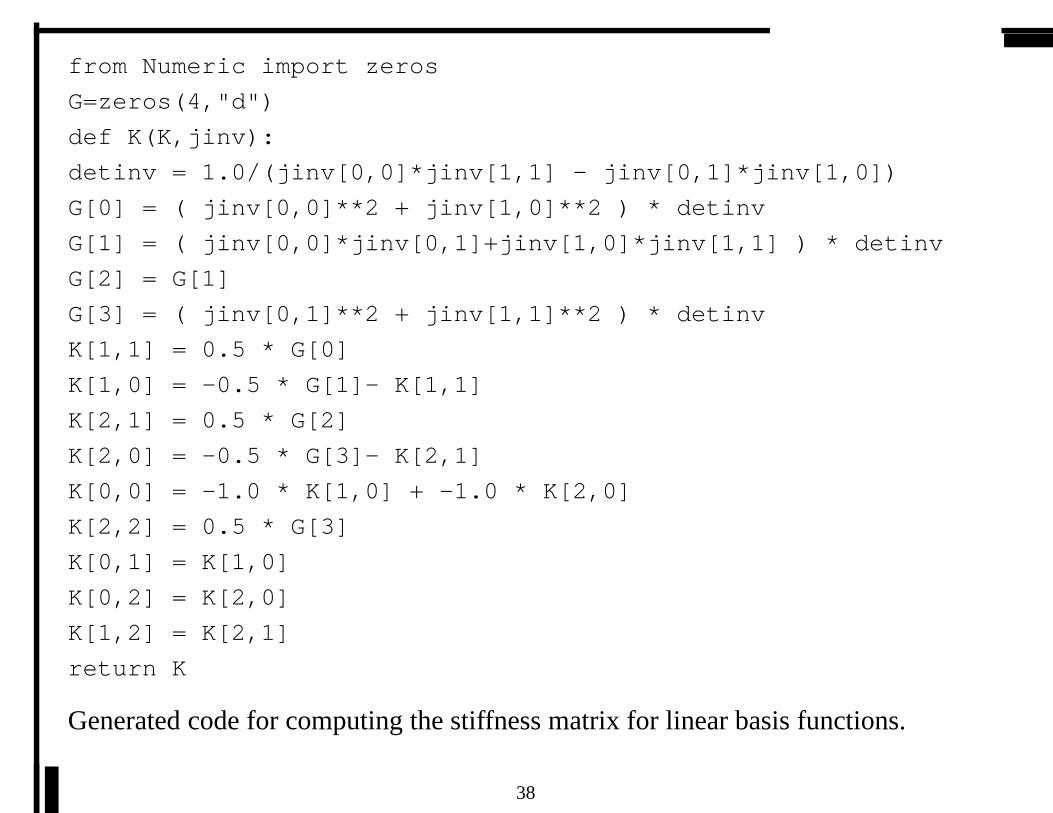
Generated code for computing the stiffness matrix for linear basis functions.

38

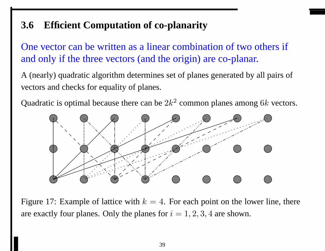
3.6 Efficient Computation of co-planarity

One vector can be written as a linear combination of two others ifand only if the three vectors (and the origin) are co-planar.

A (nearly) quadratic algorithm determines set of planes generated by all pairs of

vectors and checks for equality of planes.

Quadratic is optimal because there can be2k2 common planes among6k vectors.

Figure 17: Example of lattice withk = 4. For each point on the lower line, there

are exactly four planes. Only the planes fori = 1, 2, 3, 4 are shown.

39

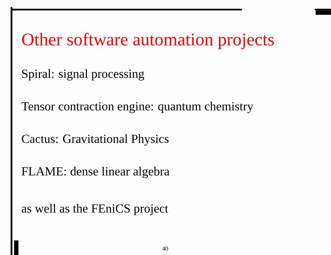
Other software automation projects

Spiral: signal processing

Tensor contraction engine: quantum chemistry

Cactus: Gravitational Physics

FLAME: dense linear algebra

as well as the FEniCS project

40

References

[1] Babak Bagheri and L. R. Scott. About Analysa. Research Report UC/CS

TR-2004-09, Dept. Comp. Sci., Univ. Chicago, 2004.

[2] Christopher Warwick Fraser.Automatic generation of code generators.PhD

thesis, 1977.

[3] Kingshuk Karuri.A Framework for Automatic Generation of Code

Optimizers. PhD thesis, 2001.

[4] Ken Kennedy, Bradley Broom, Arun Chauhan, Rob Fowler, John Garvin,

Charles Koelbel, Cheryl McCosh, and John Mellor-Crummey. Telescoping

languages: A system for automatic generation of domain languages.

Proceedings of the IEEE, 93(2), 2005. special issue on ”Program Generation,

Optimization, and Adaptation”.

[5] J. Korelc. Multi-language and multi-environment generation of nonlinear

finite element codes.Engineering with Computers, 18:312–327, Nov 2002.

10.1007/s003660200028.

41

[6] Joze Korelc. Automatic generation of finite-element code by simultaneous

optimization of expressions.Theoretical Computer Science, 187:231–248,

Nov 1997.

[7] Robert van Engelen, Lex Wolters, and Gerard Cats. CTADEL: a generator of

multi-platform high performance codes for PDE-based scientific applications.

In ICS ’96: Proceedings of the 10th international conference on

Supercomputing, pages 86–93, New York, NY, USA, 1996. ACM Press.

[8] Paul S. Wang, Hui-Qian Tan, Atef F. Saleeb, and Tse-Yung P. Chang. Code

generation for hybrid mixed mode formulation in finite element analysis. In

SYMSAC ’86: Proceedings of the fifth ACM symposium on Symbolic and

algebraic computation, pages 45–52, New York, NY, USA, 1986. ACM Press.

42