the decision to buy or lease equipment from an engineering
TRANSCRIPT

The decision to buy or lease equipment from an engineering
economics perspective
By
Cebsile Mkhatshwa
28319461
Submitted in partial fulfilment for the degree of
BACHELORS OF INDUSTRIAL ENGINEERING
In the
FACULTY OF ENGINEERING, BUILT ENVIRONMENT AND
INFORMATION TECHNOLOGY
UNIVERSITY OF PRETORIA
October 2011

1
Executive Summary
Leasing and purchasing equipment forms some of the expenses on the capital budget hence,
affects the net profit of a company. When deciding whether to lease or purchase equipment it
is essential to understand the cash flows associated with each option and the effects of certain
parameters on the cash flows in order to select the option that will give the highest return to
the investment. In this study the net present value (NPV) is used to decide whether to lease or
purchase equipment, with the help of spreadsheet models that represent the cash flows
associated with each option. Then the effect of inflation rates, project life, interest rates, loan
payback period and percentage equity used to purchase the asset on the NPVs of the
spreadsheet models is determined using sensitivity analysis.

2
Table of Contents Executive Summary ................................................................................................................................ 1
CHAPTER 1: Introduction and Background .......................................................................................... 4
1.1 Background and Problem Statement ....................................................................................... 4
1.2 Project Aim ............................................................................................................................. 4
1.3 Project Scope .......................................................................................................................... 5
Chapter 2: Literature Review .................................................................................................................. 6
2.1 Capital Budget ........................................................................................................................ 6
2.1.1 Importance of the capital budget ................................................................................... 6
2.1.2 Influence of the capital structure on capital budget decisions ........................................ 6
2.1.3 Influence of interest, tax and inflation rates on cost of capital ....................................... 7
2.2 Lease of Equipment ................................................................................................................ 8
2.2.1 Typical lease agreement .................................................................................................. 8
2.2.2 Different types of leases available .................................................................................. 8
2.2.3 Tax and leasing agreements ............................................................................................ 9
2.2.4 Influence of interest changes on a lease agreement ........................................................ 9
2.3 Purchasing of equipment ....................................................................................................... 10
2.3.1 Tax implications ............................................................................................................ 10
2.3.2 Depreciation .................................................................................................................. 10
2.4 Existing methodologies of making the lease-buy decision ................................................... 10
Chapter 3: Solution ............................................................................................................................... 13
3.1 Engineering methods and tools ............................................................................................. 13
3.2 Method selection and development..................................................................................... 14
Chapter 4: Analysis ............................................................................................................................... 22
Chapter 5: Conclusions ......................................................................................................................... 31
APPENDIX A – Purchasing models with different equity ................................................................... 32
APPENDIX B – Purchasing models with varying project life ............................................................. 36
APPENDIX C- Purchasing models with different pay back periods .................................................... 40
APPENDIX D-Purchasing models with different inflation rates ......................................................... 43
APPENDIX E- Leasing models with different inflation rates .............................................................. 46
APPENDIX F- leasing models with varying project lives .................................................................... 49

3
Appendix G – purchasing models with varying interest rates .............................................................. 52
Appendix H- leasing models with varying interest rates ....................................................................... 55
Bibliography ......................................................................................................................................... 58
List of tables
TABLE 1: INPUT DATA TO THE PURCHASE SPREADSHEET MODEL ...................................................................... 16
TABLE 2: PURCHASING SPREADSHEET MODEL ................................................................................................... 18
TABLE: 3 INPUT DATA FOR THE LEASING SPREADSHEET MODEL ....................................................................... 20
TABLE: 4 SPREAD SHEET THAT REPRESENTS THEN LEASING OPTION ................................................................ 20
TABLE 5: NPV AND EQUITY ................................................................................................................................ 23
TABLE: 6 CHANGE IN NPV AS THE PROJECT LIFE VARIES ............................................................................... 24
TABLE 7: NPV FOR VARYING PAYBACK PERIODS ............................................................................................... 25
TABLE 8: NPV AND INFLATION RATES WHEN PURCHASING ............................................................................................... 26
TABLE 9: NPV ASSOCIATED WITH DIFFERENT INFLATION RATES WHEN LEASING ........................................... 27
TABLE 10: NPV FOR DIFFERENT PROJECT DURATIONS IN THE LEASING OPTION ............................................. 28
TABLE 11: NPV FOR DIFFERENT INTEREST RATES ............................................................................................. 29
TABLE 12: NPV AND DIFFERENT INTEREST RATES WHEN THE ASSET IS LEASED .............................................. 30
List of figures
FIGURE 1: HYDRAULIC MIXER ................................................................................................................................................. 15
FIGURE 2: SENSITIVITY ANALYSIS OF NPV TO THE VARIATION IN THE % OF EQUITY USED TO PURCHASE THE ASSET .......... 22
FIGURE 3: SENSITIVITY ANALYSIS OF NPV TO THE VARIATION IN PROJECT LIFE IF ASSET IS PURCHASED ............................. 24
FIGURE 4: SENSITIVITY ANALYSIS OF NPV TO THE VARIATION IN PAYBACK PERIODS IF ASSET IS PURCHASED ...................... 25
FIGURE 5: SENSITIVITY ANALYSIS OF NPV TO THE VARIATION IN INFLATION IF THE ASSET IS PURCHASED........................... 26
FIGURE 6: SENSITIVITY ANALYSIS OF NPV TO THE VARIATION IN INFLATION RATES IF ASSET IS LEASED .............................. 27
FIGURE 7: SENSITIVITY ANALYSIS OF NPV TO THE VARIATION IN PROJECT LIFE IF THE ASSET IS LEASED............................. 28
FIGURE 8: SENSITIVITY ANALYSIS OF THE AFFECT OF INTEREST RATE ON THE NPV AN ASSET IS PURCHASED ...................... 29
FIGURE 9: SENSITIVITY ANALYSIS OF THE AFFECT OF INTEREST RATE ON THE NPV AN ASSET IS LEASED ............................. 30

4
CHAPTER 1: Introduction and Background
1.1 Background and Problem Statement Prior to the 1950s only land and buildings were leased. Today, however almost any fixed
asset can be leased. For example about 50% of all new commercial aircraft sold is purchase
by aircraft leasing companies (Brigham et al., 1999).
At times companies make the decision to buy or lease equipment while not taking into
account all the factors that will have a positive or negative effect on the cash flow associated
with the decision made. This could be due to the fact that the management of a trading entity
may not be aware of the long term impact that acquiring an asset through leasing or buying
has on the capital budget of the company.
Most published literature that discusses the decision to lease or purchase equipment only
addresses the matter from a certain perspective and hence leaves out other factors that are
relevant to management faced with the task of deciding to lease or purchase equipment. For
example some publications present mathematical models that can be used to decide whether
to lease or purchase equipment but leaves out the detailed theoretical explanations of the cash
flows incorporated into the formulas of the models and the effect that these cash flows will
have on the capital budget of the company, which is what management is interested in. These
models can prove to be of little help since they can be difficult to understand and implement
and require extensive mathematical knowledge to solve them.
There is a great need for a comprehensive analysis of leasing and purchasing equipment and a
simplified approach of deciding whether to lease or purchase equipment that will be relevant
and easy to implement for all companies.
1.2 Project Aim The aim of this study is to provide a detailed research on the following:
The cash flows associated with leasing and purchasing equipment.
The factors that companies should consider when contemplating to lease or purchase
equipment.
The effect that leasing and purchasing equipment has on a company’s capital budget.
Then finally provide a structured approach that can be followed by any company when
deciding to lease or purchase equipment.

5
1.3 Project Scope To conduct the study the following problem solving approach will be used (Tarquin, 2008:8)
Step 1: understand the problem.
Step 2: Collect information.
Step 3: Define feasible alternative solution and make realistic estimations.
Step 4: Identify criteria for decision making.
Step 5: Evaluate each alternative.
Step 6: Select the best alternative.
To accomplish the first two steps, an in depth study of the literature currently available about
buying and leasing equipment and how the capital budget is affected by leasing or purchasing
equipment. The effect that the size of the loan acquired to purchase the equipment, period to
pay back the loan, inflation rate and project life on the decision to purchase or lease
equipment.
With regards to step 3; the alternative solutions will be the different techniques of evaluating
capital investment decisions. Keep in mind that the solution in this case would be the best
suited technique to be used when deciding to lease or purchase equipment.
According to step 4, a decision making criteria must be selected for each technique
mentioned in step3.
In step 5 each decision making technique will be evaluated and compared against each other.
Lastly a conclusion will be reached on which technique is to be used when deciding to lease
or purchase equipment.

6
Chapter 2: Literature Review
2.1 Capital Budget A capital budget consists of an outline of planned long term investments on fixed assets.
Capital budgeting is the process of analyzing projects and deciding which ones to include in
the company’s capital budget. Assets included in the capital budget have the following
characteristics (du Toit et al., 2001):
The expected life of the asset is longer than one year.
They are not traded in the normal course of the firm’s business.
The equipment to be discussed in this study present the features or characteristics mentioned
above therefore they are recorded in the capital budget and can be referred to as capital
budget investments.
2.1.1 Importance of the capital budget The distribution of resources in the capital budget determines whether management will
be able to produce a minimum return on the investor’s money that the investor would
have received on an alternative investment. This factor determines whether investors keep
investing in the company or they take their investments elsewhere (Brigham et al.,2005).
From the capital budget potential investors and current investors can determine the firm’s
strategic direction.
The acquisition of assets or projects that the company decides to finance will affect the
company’ cash flow for a number of years still to come, that is why capital budgeting is
preceeded by a forecast of future expences and future income. A significant amount of
this forecast is done during the analysis of the cash flows associated with leasing or
purchasing equipment.
2.1.2 Influence of the capital structure on capital budget decisions
To acquire an asset buy leasing or purchasing a company needs capital. Capital structure
refers to the different sources of capital that a company uses, the fixed amount of capital
that the company gets from each source and the cost of each capital source. These
different sources of capital are referred to as capital components. According to Brigham
et al., (1999) the three major capital components are: common stock, preferred stock and
debt capital. Companies may choose to use only one of these sources of capital or a
combination of two sources or a combination of all three sources.

7
Common stock refers to the amount that shareholders have invested in the organisation
plus retained earnings, which is the amount earned from income generating activities
(Walter & Charles, 2008). Preferred stock is a hybrid of common stock and long-term
debt. Preferred stock can be referred to as long term debt because if it is used as capital to
acquire an asset then a fixed dividend must be paid to the preferred stockholders. It can
also be referred to as common stock because the dividend is not paid out to the preferred
stock holders unless the board of directors declare the dividend, as this is the case with
common stock (Walter & Charles, 2008). Debt capital refers to raising capital by
acquiring debt; it can be through a loan or issuing bonds. Each company ought to have an
optimal capital structure that is aimed at providing the highest possible economic value
added (EVA).
According to Brigham et al., (1999) the capital structure is used to determine the cost of
capital by using the weighted average cost of capital equation (WACC).
WACC = 𝒘𝒅𝒌𝒅 𝟏 − 𝑻 + 𝒘𝒑𝒔𝒌𝒑𝒔 + 𝒘𝒄𝒆𝒌𝒔 [𝟐. 𝟏]
wd, wps and wce are the weights used for debt, preferred and common equity respectively.
kd is the interest rate of the debt.
T is the marginal tax of the firm.
Kps is the preferred dividend divided by the net issuing price, 𝑘𝑝𝑠 = 𝐷𝑝𝑠
𝑃𝑛
Ks is the rate of return required by investors.
The weights for debt, preferred equity and common equity are determined by each
company on the company’s capital structure policy.
Capital structure enables management to determine beforehand the projects that will
require a minimum cost of capital. By considering the capital structure management can
determine the capital component that costs the most at that specific time, and then use less
of that capital component when financing new capital investments.
2.1.3 Influence of interest, tax and inflation rates on cost of capital
When interest rates in the economy increase the cost of debt capital will also increase
because bondholders and banks will require a higher interest rate. Higher interest rates
will also increase the cost of preferred equity capital. Variation in the tax rate will affect
the cost of capital equity. An increased tax rate will lead to a low cost of debt capital
according to the WACC equation (Brigham et al., 1999). An increase in inflation tends to

8
increase the required rates of return by the investors, this leads to a higher cost of capital
(du Toit et al., 2001).
2.2 Lease of Equipment
2.2.1 Typical lease agreement
Leasing is characterised by the separation of ownership of the asset and right of use of the
asset between the lessor and the lessee. The lessor owns the asset but the lessee has the right
to use the asset (du Toit et al., 2001). According to the Internal Revenue Service an
agreement is regarded as a lease agreement if the following requirements are met (Brigham
1999):
The period of leasing the asset (including renewals and extensions of the lease
agreement) should not exceed 80% of the estimated useful life of the asset. The
remaining useful life of the asset after the lease term must not be less than a year.
The residual value of the asset at the end of the lease term must at least equal 20% of
the value of the asset at the start of the lease period.
The lessee or any other party is not allowed to purchase the equipment at a price
determined at the start of the lease term.
A lease agreement usually contains the following information:
The duration of the lease contract.
The specific lease payments and the number of payments.
Conditions of renewal of the lease agreement.
Individual responsible for maintenance costs.
How the residual value will be incorporated in the cash flows.
The description of the leased assets.
2.2.2 Different types of leases available
Leasing takes place in four different forms, being, the operating lease, financial or capital
lease and a sale and sale back lease agreement (Brigham et al., 1999).
Operating lease
The lessor is required to maintain and service the leased equipment, the cost of
maintaining is built into the lease payment.
The lease payments are not sufficient for the lessor to cover the full capital
coat of the asset.
Operating lease agreements contain a cancellation clause which allows the
lessee to cancel the lease and return the asset before the end of the lease term.

9
Financial or capital lease
The lessor does not provide maintenance services.
The lease payments fully amortize the capital cost of the equipment.
The lease agreement is not cancellable, unless the asset is fully amortized.
Sale – and - Leaseback
A company that owns an asset sells the asset to another firm and
simultaneously executes an agreement to lease the equipment at specific terms
and period.
The seller gets the purchase price immediately from the buyer.
The seller still retains the use of the equipment.
2.2.3 Tax and leasing agreements
According to the Income Tax Act 1962, administered by the Commissioner of the South
African Revenue Services (SARS), tax payments and other expenditures incurred in the
production of income not of capital nature can be deducted from income for tax purposes.
These deductions grant tax savings for the lessee and are referred to as general deductions.
The tax savings are calculated in the following manner:
𝑻𝒂𝒙 𝒓𝒂𝒕𝒆 × 𝒍𝒆𝒂𝒔𝒆 𝒑𝒂𝒚𝒎𝒆𝒏𝒕 + (𝑶𝒕𝒉𝒆𝒓 𝒆𝒙𝒑𝒆𝒏𝒅𝒊𝒕𝒖𝒓𝒆𝒔 × 𝑻𝒂𝒙 𝒓𝒂𝒕𝒆) [2.2]
2.2.4 Influence of interest changes on a lease agreement
Interest rates influence the lease payments determined by the lessor on the lease agreement.
The internal rate of return (IRR) that will allow the net present value of the cash flows
experienced by the lessor equal to zero is the IRR that the lessor selects to determine the lease
payments.
The lessor determines the internal rate of return (IRR) required by considering the net
present value of the cash flows experienced while acquiring the asset and maintaining it.
These cash flows from the lessor perspective include: the net purchase price, maintenance
costs, tax on residual value and lease payment, depreciation and maintenance tax savings.
If the cost of capital (return required by the capital components) for acquiring and maintain
the asset was high, this will result in the lessor declaring a high IRR in order to pay back the
cost of capital and earn interest. This will result in high lease payments.
On the other hand if the return required by the capital components is relatively low, the lessor
will declare a lower IRR, hence the lease payments on the lease agreement will be lower
(Brigham et al., 1999).

10
2.3 Purchasing of equipment
2.3.1 Tax implications
According to the Legal and Policy division, South African Revenue Service (2009) all goods
purchased from a vendor value added tax (VAT) is paid as part of the purchase price. The
current vat rate is 14% is South Africa. Therefore when purchasing an asset, the VAT is
included in the purchase prize. Once the asset is purchased and put to use, the tax payer can
declare tax savings based on the operating expenses of the asset and depreciation expenses
(S.A Income tax Act section 6, 1962). If the asset is being resold at a market value that is
higher than the salvage value, a capital gains tax (CGT) is paid on the difference between the
two amounts (South African Income tax Act section 11, 1962).
2.3.2 Depreciation Depreciation refers to the reduction in the value of an asset (Tarquin, 2008). Depreciation
reduces the calculated net profit even though it is not a cash charge. A high depreciation leads
to a low tax bill (Brigham, 1999). Depreciation can be calculated using one of the following
methods
Straight line depreciation: The difference between the initial purchase price of the
asset and the estimated salvage value is divided by the economic life of the project to
find the annual depreciation amount (Tarquin, 2008). This method is mainly used for
stockholder reporting (or book purposes) (Brigham, 1999).
Modified accelerated cost recovery system (MACRS): This method consists of two
steps. In the first step the annual depreciation is determined by multiplying the initial
cost of the asset. In the second step, the book value in a particular year is determined
by subtracting the sum of annual depreciations (from previous years) from the initial
purchase price of the asset (Tarquin, 2008). This method is favoured when calculating
income tax since it yields high net profit reductions due to high depreciation
(Brigham, 1999).
2.4 Existing methodologies of making the lease-buy decision Various tools have been suggested to assist companies make the right choice to lease or
purchase equipment. The Vincil model also known as the Lease-Or-Borrow model is one of
these tools (Sartoris & Paul, 1973, 46:52). The Lease-Or-Borrow model compares the cost of
acquiring an asset through lease financing to the cost of acquiring the asset by purchasing the
asset using debt capital. The first step of the Lease-Or-Borrow model is to determine the net
present value of owning an asset, using the following formula
11
𝑵𝒆𝒕 𝒑𝒓𝒆𝒔𝒆𝒏𝒕 𝒗𝒂𝒍𝒖𝒆 𝒐𝒇 𝒑𝒖𝒓𝒄𝒉𝒂𝒔𝒆 = −𝑪 + 𝑫𝒏𝒕
(𝟏 + 𝒊)𝒏
𝒌
𝒏+𝟏
[𝟐. 𝟑]
Where C = Purchase Price
Dnt = Depreciation tax savings in year n
t = tax rate
i = Cost of capital
K = Life of the project
The second step is to determine the net present value of the lease payments, using the
following equation:
𝑵𝒆𝒕 𝑷𝒓𝒆𝒔𝒆𝒏𝒕 𝑽𝒂𝒍𝒖𝒆 𝒐𝒇 𝒍𝒆𝒂𝒔𝒆 = 𝑨𝒏𝒕
(𝟏+𝒊)𝒏𝒌𝒏=𝟏 −
𝑳𝒏
(𝟏+𝒓)𝒏𝒌𝒏=𝟏 [𝟐. 𝟒]
Where An = non interest portion of the lease payment in year n.
Ln = Lease payment in year n.
r = Basic interest rate.
k = Life of the asset.
i = Cost of capital
The highest positive NPV between the NPV of the lease and the NPV of purchasing indicates
the best alternative of acquiring the asset.
The Lease-Or-Buy model was developed by Johnson & Wilbur (1972). This model is similar
to the Lease-Or-Borrow model because it also develops the NPVs associate with leasing and
owning equipment. The difference between the two models is that the Lease-Or-Buy model
includes costs that are common when leasing or purchasing equipment, on the other hand the
Lease-Or-Borrow model omits these costs. Another significant difference between the two
models is that the Lease-Or-Buy model compares the costs of acquiring an asset through
leasing to the costs of acquiring through purchasing using own equity. On the other hand the
Lease-Or-Borrow model compares leasing to purchasing using debt capital.
The Lease-Or-Buy model consists of the following equations
𝑵𝑷𝑽 𝒑𝒖𝒓𝒄𝒉𝒂𝒔𝒆 = −𝑪 + 𝒕𝑫𝒏
(𝟏+𝒊)𝒏𝒌𝒏=𝟏 +
𝑹𝒏 (𝟏+𝒕)
(𝟏+𝒊)𝒏𝒌𝒏=𝟏 [2.5]

12
𝑵𝑷𝑽 𝒍𝒆𝒂𝒔𝒆 = 𝑹𝒏 +𝑶𝒏 (𝟏−𝒕)
(𝟏+𝒊)𝒏𝒌𝒏=𝟏 −
𝑳𝒏(𝟏−𝒕)
(𝟏+𝒓𝒕𝒊)𝒏𝒌𝒏=𝟏 [2.6]
Where Ri = Operating cash flow from the project in year i.
Oi = Operating costs that would occur under ownership of the asset but not under
the lease agreement.
rt = after tax interest rate.
Ln = Lease payment in year n.
Sartoris & Paul (173, 46:52) compared the two models (Lease-Or-Borrow and Lease-Or-
Buy) and reached a conclusion that Lease-Or-Borrow model leads to the correct decision
while Lease-Or-Buy model leads to an incorrect decision.

13
Chapter 3: Solution
3.1 Engineering methods and tools Leasing and purchasing equipment are both capital budget investments. Brigham et al.,(1999)
define the following capital budgeting decision rules that should be used to decide whether a
capital investment should be included in the capital budget or not.
Payback period – Compares the number of years required to recover the investment in
each project. The project with the lowest payback period is selected. It is applicable to
mutually exclusive projects.
𝑵𝒖𝒎𝒃𝒆𝒓 𝒐𝒇 𝒚𝒆𝒂𝒓𝒔 = 𝑰𝒏𝒊𝒕𝒊𝒂𝒍 𝑰𝒏𝒗𝒆𝒔𝒕𝒎𝒆𝒏𝒕
𝑨𝒏𝒏𝒖𝒂𝒍 𝒏𝒆𝒕 𝒄𝒂𝒔𝒉 𝒇𝒍𝒐𝒘 [𝟑. 𝟏]
Net Present Value (NPV) – NPV refers to the sum of the discounted cash flows at the
cost of capital. If NPV = 0, then the project is acceptable because the cash inflow is
sufficient to repay the initial investment at required rate of return of the capital. If
NPV > 0, then the project is still acceptable since the cash inflows will pay back the
cost of capital at a rate higher than the required cost of capital. If NPV < 0 then the
project is not acceptable since capital will be repaid at a rate that is less than the
required rate of return.
IRR (internal rate of return) –IRR is the rate of return required by a company to
ensures that the NPV of cash inflows is equal to zero. If the rate of return of any
project is less than the IRR of the company then that project is not included in the
capital budget.
MIRR (modified internal rate of return) – This decision making rule is an
improvement of the IRR. When using this rule, the terminal value (TV) has to be
defined. The TV is the future value of cash inflows. The MIRR is the discount rate
that ensures that the present value of cash outflows (PV cost) is equal to the present
value of the terminal value.
Profitability Index (Benefit cost ratio) – Shows the relative profitability of a project. A
project is acceptable if the Profitability index is greater than 1.0.
𝑷𝑰 = 𝑷𝑽 𝒃𝒆𝒏𝒆𝒇𝒊𝒕𝒔
𝑷𝑽 𝑪𝒐𝒔𝒕 [𝟑. 𝟐]

14
Brigham et al.,(1999) further mention that the net present value decision rule is the most
reliable and accurate decision rule.
3.2 Method selection and development To compare purchasing equipment and leasing equipment a cash flow analysis is used and the
cash flows are presented on spreadsheet models. This method is selected because it is easier
to prepare and understand spreadsheet models than to set up and understand mathematical
models. Hence, this method can be applied by any company. The NPV rule is used to analyse
the spreadsheets that represent the options of leasing and purchasing equipment in this study
because according to Brigham et al., (1999) this is the rule that managers prefer to use when
comparing projects. The reason for this is that the NPV value directly links to the economic
value added (EVA) to the company by a certain project and this is the information that
shareholders and investors are interested in. For example the NPV refers to the present value
of the EVA (Brigham et al., 1999). Brigham et al., (1999) further mentioned that well
managed companies cannot purchase equipment cash because cash is usually tied up in
assets.
To implement the method mentioned in the paragraph above, the following steps must be
followed.
I. State assumptions.
II. Collect the information that will be used to develop the spreadsheet models.
III. Present the expected cash flows on spreadsheet models.
IV. Determine the net present value in each of the spreadsheet models and decide on the
best alternative. The alternative with the highest positive NPV value will be accepted.
If the NPV value derived from the spread sheet calculations is negative, the option
represented by that spreadsheet is not accepted.
V. Determine how some inputs of the spreadsheet models affect the NPV, by changing
one input variable while keeping all other parameters and variables the same.
The final step is optional. It can be done if the company would like to know how certain
parameters will affect the cash flows associated with leasing and the cash flows associated
with purchasing. This step will be demonstrated in chapter 4.
To test this methodology, the steps listed above were used to decide whether to purchase or
lease an asset called the hydraulic mixer with scale (see figure 1). The relevant information
about the hydraulic mixer (e.g. purchase price, lease payments, operating costs) was made
available by the Turner and Morris Company located in Pretoria town Skinner Street. The
trade of the Turner and Morris Company is to sell and lease out fixed assets that are used in
the construction industry.

15
Figure 1: Hydraulic mixer
I. State assumptions
A loan is used to finance the purchase of the asset.
Payback period of the loan is 4 years.
The market value of the asset once it has been purchased decreases at a 10%
rate.
Life of the project is 15 years.
The minimum allowed rate of return (MARR) of the company is 15% since it
is normally stated to be higher than the rate of return charged by banks.
The lease presented on the spreadsheet model is an operating lease whereby
the lessor is responsible for the overhaul maintenance cost but the lessee is
responsible for the daily maintenance cost.

16
II. Collect relevant information
The data that is used to prepare the spread sheet models is presented on input tables
and calculations that precede each spread sheet model.
Steps III & IV are presented simultaneously on the spreadsheet models.
Below is the input table which represents data used to prepare the spreadsheet model that
represents the purchasing alternative.
Table 1: Input data to the purchase spreadsheet model
Cash Flow Analysis for purchasing a hydraulic mixer using a loan.
Scenario: Purchase equipment using a loan.
Input table
Purchase price + VAT 254 218.86
Loan Amount 254 218.86
Interest on loan (i) 7.00%
Payback period 4 years
Normal tax rate 28%
Secondary tax 10%
Life of project 15 years
Tax life 3 years

17
Calculations:
Annuity, A (n = 4) P(A/P,7,4)
Depreciation per year: R 75 053.03
(254218.86 - 40 000)/3
R 71 406.28667
Annual interest (n = 4) : A(P/A,7,n)*7% Interest in year 1 17795.37
Annual Income :
Interest in year 2 13787.32
each load = 5 litres at R50 per 5 litres
Interest in year 3 9498.71
In one hour = 4 loads
Interest in year 4 4910.12
operates for 8 hours 6 days per week Assume 52 weeks per year
(6*52*8)*(4*50)
Annual operating expenses
R 499200 diesel (R11 per hour) 440
2 labourers (R18 per hour) 89856 1 Operator ( R35 per hour) 87360
MARR After tax Engine oil and filter service 2000
MARR Before Tax = 15%
Total R 179656
MARR(Before tax) (1 - Tax rate) Assumption: work 8 hrs 6 days a week
0.108
Overhaul service every 3 years R 50 000
11%
Market Value After 15 years: 254 218.86 *( 1- g)^(15-1); g = 10%
58157.12098
The purchase price of this asset was provided by the Turner and Morris Company.
The loan used to purchase this equipment covers the entire purchase price. According
to Brigham et al., (1999) well managed companies cannot afford to purchase such
equipment cash since the company’s cash is tied up in fixed assets. The effect that the
percentage of own equity used to purchase the equipment is still to be investigated
further in this study.
The annuities and interest rates were calculated using discount factors published by
Blank Tarquin (2008).
The interest rate on the loan is 7% as this is the official rate of interest published by the
Legal and Policy division South African Revenue Services, March 2011.

18
The MARR before tax is 15% and it is based on the interest rate charged by the banks.
The MARR expected by management in companies is always higher that the interest
charged by the banks in order to declare a profit.
The depreciation used is straight line depreciation (Brigham et al., 1999:446)
The tax life of this equipment (cement mixer) is 3 years as stated on the Binding
General Ruling (Income Tax Act): NO.7 published 11 April 2011.
The Normal and Secondary tax rates are as published by the South African Revenue
Services.
To determine the market value at the end of the life of the project, it was assumed that
the market value decreases by 10% per year. The formula used is stated under
calculations.
The operating expenses and income are specific to the equipment being evaluated.
Below is the spreadsheet model that represents the option of purchasing the asset.
Table 2: Purchasing Spreadsheet model
Year
CFBT
Depreciation
Book
Value
Loan
Interest
Operating
cost
and
maintenance
Taxable
Income
Loan
Payment
Tax
payment
CFAT
0
1 499200 -71072.95 183,145.91 17795.37 179656 230675.67 75,053.03 64,589.19 179901.78
2 499200 -71072.95 112,072.95 13787.32 179656 234683.73 75,053.03 65,711.44 178779.52
3 499200 -71072.95 41,000.00 9498.71 R 229,656 R 188,972.33 75,053.03 52,912.25 R 141,578.71
4 499200 4910.12 179656 R 314,633.88 75,053.03 88,097.49 R 156,393.48
5 499200 179656 319544 89,472.32 230,071.68
6 499200 R 229,656 269544 75,472.32 R 194,071.68
7 499200 179656 319544 89,472.32 R 230,071.68
8 499200 179656 319544 89,472.32 R 230,071.68
9 499200 R 229,656 269544 75,472.32 R 194,071.68
10 499200 179656 319544 89,472.32 R 230,071.68
11 499200 179656 319544 89,472.32 R 230,071.68
12 499200 R 229,656 269544 75,472.32 R 194,071.68
13 499200 179656 319544 89,472.32 R 230,071.68
14 499200 179656 319544 89,472.32 R 230,071.68
15 499200 R 229,656 269544 75,472.32 R 194,071.68
MV 58,157 41,000.00 17,157.12 4,803.99 R 53,353.13
NPV:
179 901.78(P/F,11,1) + 178 779.52(P/F,11,2) + 141 578.71(P/F,11,3) + 156 393.48(P/F,11,4) + 230 071.68(P/F,11,5)
194 071.68(P/F,11,6) + 230 071.68(P/A,11,2)(P/F,11,6) + 194 071.68(P/F,11,9) + 230 071.68(P/A,11,2)(P/F,11,9)
+ 194 071.68(P/F,11,12) + 230 071.68(P/A,11,2)(P/F,11,12) + 194(P/F,11,15) + 53 353.13(P/F,11,15)

19
1414270.19
EAA (Equivalent Annual Annuity) = P(A/P,11,15)
196682.556
All cash flows are considered to be at the end of the year.
CFBT refers to cash flow before tax, and CFAT refers to cash flow after tax
The CFBT is the income generated by the equipment; in this case it is determined
under calculations.
The depreciation is calculated as stated on the calculations above.
The taxable income is calculated by subtracting the tax saving from depreciation and
expenditure and loses actually incurred during the year of assessment in the
production of income not of a capital nature (Income Tax Act, 1962) from the gross
income. In this case these expenses include the interest rate on the loan and operating
expenses.
𝑫𝒆𝒑𝒓𝒆𝒄𝒊𝒂𝒕𝒊𝒐𝒏 𝑻𝒂𝒙 𝒔𝒂𝒗𝒊𝒏𝒈𝒔 𝒂𝒕 𝒕𝒉𝒆 𝒆𝒏𝒅 𝒐𝒇 𝒕𝒉𝒆 𝒚𝒆𝒂𝒓 =
𝑫𝒆𝒑𝒓𝒆𝒄𝒊𝒂𝒕𝒊𝒐𝒏 𝒑𝒆𝒓 𝒚𝒆𝒂𝒓 × 𝑻𝒂𝒙 𝒓𝒂𝒕𝒆 [𝟑. 𝟑]
𝑶𝒕𝒉𝒆𝒓 𝒆𝒙𝒑𝒆𝒏𝒄𝒆𝒔 𝒕𝒂𝒙 𝒔𝒂𝒗𝒊𝒏𝒈𝒔 =
𝑬𝒙𝒑𝒆𝒏𝒄𝒆𝒔 × 𝒕𝒂𝒙 𝒓𝒂𝒕𝒆 [𝟑. 𝟒]
The loan payment is computed as stated under calculations. This amount includes
both the interest on the loan and the principle amount.
𝑻𝒂𝒙 𝒑𝒂𝒚𝒎𝒆𝒏𝒕 = 𝑻𝒂𝒙𝒂𝒃𝒍𝒆 𝒊𝒏𝒄𝒐𝒎𝒆 × 𝟎. 𝟐𝟖 [𝟑. 𝟓]
𝑪𝑭𝑨𝑻 =
𝑻𝒂𝒙𝒂𝒃𝒍𝒆 𝒊𝒏𝒄𝒐𝒎𝒆 − 𝒕𝒂𝒙 𝒑𝒂𝒚𝒎𝒆𝒏𝒕 − 𝒍𝒐𝒂𝒏 𝒑𝒂𝒚𝒎𝒆𝒏𝒕 + 𝒅𝒆𝒑𝒓𝒆𝒄𝒊𝒂𝒕𝒊𝒐𝒏 +
𝒍𝒐𝒂𝒏 𝒊𝒏𝒕𝒆𝒓𝒆𝒔𝒕. [𝟑. 𝟔]
After the life of the project (15 YEARS) the market value of the equipment is higher
than the book value (40 000). Capital gains tax is paid on the difference between the
market value and book value. The capital gains tax was assumed to be 28% of the
difference between the book value and the market value.
The NPV for the option to purchase equipment using a loan to finance it is positive,
which means that this option is acceptable.

20
Next, the option of leasing the asset is considered. Steps III & IV will be presented in the
same manner as in the option of purchasing the asset.
Table: 3 Input data for the leasing spreadsheet model
Scenario: Acquiring equipment through leasing
Input table
Purchase price +
VAT
254 218.86
Annual lease
payment
215 162.46
Normal tax rate 28%
Secondary tax 10%
Life of project 12 years
Tax life 3 years
Table: 4 Spread sheet that represents then leasing option
Year CFBT lease payment Operating cost Taxable Tax CFAT
and maintenance Income payment
0 -215162.46
1 499200 430324.92 179656 -110780.92 -110780.92
2 499200 215162.46 179656 104381.54 29226.8312 75154.7088
3 499200 215162.46 179656 104381.54 29226.8312 75154.7088
4 499200 215162.46 179656 104381.54 29226.8312 75154.7088
5 499200 215162.46 179656 104381.54 29226.8312 75154.7088
6 499200 215162.46 179656 104381.54 29226.8312 75154.7088
7 499200 215162.46 179656 104381.54 29226.8312 75154.7088
8 499200 215162.46 179656 104381.54 29226.8312 75154.7088
9 499200 215162.46 179656 104381.54 29226.8312 75154.7088
10 499200 215162.46 179656 104381.54 29226.8312 75154.7088
11 499200 215162.46 179656 104381.54 29226.8312 75154.7088
12 499200 179656 319544 89472.32 230071.68
NPV:
- 110 780 (P/F,11,1)+ 75 154.709*(P/A,11,10) (P/F,11,1)+ 230 071.68*(P/F,11,12)
364691.2973

21
EAA (Equivalent Annual annuity) = P(A/P,11,12)
56173.40053
The lease payment is always paid at the beginning of the year. However, the first
lease payment can be paid along with the second payment at the beginning of the first
year.
Lease payments are considered to be an expense, hence, there are tax savings
experienced due to lease payments. Equation [3.4] was used to determine the tax
savings associated with the lease payment.
The value of operating expenses represents the expenses experienced daily, not the
overhaul expenses. This value was calculated in the calculations preceding the
spreadsheet model that represents the purchasing option. Equation [3.4] was used to
determine the tax savings associated with this expense.
The NPV is positive which makes this alternative acceptable.
When considering the NPV values on the spreadsheets we notice that the NPV on the
spreadsheet that represents purchasing is higher (R 1 414 270.19) than the NPV valve on the
spreadsheet that represents leasing (R 364 691.2973). These values suggest that the
purchasing alternative should be implemented. According to the NPV rule the alternative
with the highest positive NPV should be implemented. However, there is still another factor
to consider; the lives of the projects are not the same. In order to compare projects with
different lives the Equivalent Annual Annuity (EAA) value should be used (Brigham et al.,
1999). In each spreadsheet the EAA value is calculated right after the NPV value. The option
with the highest positive EAA value should be chosen. The EAA of the purchasing
calculations is R 1960682.556 and the EAA value of the leasing calculations is R
560173.40053. The purchasing option has a higher EAA value which means the asset should
be purchased rather than leased.

22
Chapter 4: Analysis
To accomplish step V sensitivity analysis was carried out on both spreadsheet models, to
determine how certain parameters affect the cash flows associated with leasing and
purchasing.
To determine how the percentage of own equity used to purchase the equipment affects the
NPV, different purchasing spreadsheet models were prepared where the amount of own
equity used to purchase the asset varied from 0% of the purchase price to 100% of the
purchase price. The spreadsheet model representing 0% own equity can be seen on table 2
and the spreadsheet models representing 25% to 100% own equity can be found in appendix
A. From figure 2 it can be seen that when the percentage of own equity used to finance the
purchase price increases, the NPV or profit that is expected from a project will decrease at a
constant rate. This shows that it would be best to purchase the asset using a loan rather than
use own equity (company’s money) to purchase the equipment.
Figure 2: Sensitivity analysis of NPV to the variation in the % of equity used to purchase the asset
1360000
1370000
1380000
1390000
1400000
1410000
1420000
0% 25% 50% 75% 100%
NP
V
% of own equity used to purchase equipment
Change in NPV as equity changes
NPV

23
Table 5: NPV and Equity
NPV Equity
1414270 0%
1406336 25%
1398381 50%
1390413 75%
1382446 100%
Figure 3, below demonstrates how the NPV of a project changes if the duration of the project
decreases, when the asset is purchased using a loan. When the project life is varying the
market value of the asset at the end of the project life is affected, as well as the total income
generated since the number of operating years is varying. A project life of 15 years is the
normal scenario depicted on table 2, for further investigation the project life was reduced to 3
years (these spreadsheet models are shown in appendix B). On figure 3 it can be shown that
as the project life decreases from 15 years to 3 years the NPV or the return on the project
decreases. This is simply because the number of operating years has decreased hence less
profit is made.

24
Figure 3: Sensitivity analysis of NPV to the variation in project life if asset is purchased
Table: 6 Change in NPV as the project life varies
Project life NPV
3 812085.39
6 875706.2996
9 1141355.46
12 1179742.949
15 1223340.701
The graph bellow (figure 4) depicts how the payback period of a loan used to purchase an
asset affects the NPV. The payback period is increased from 4 years to 8, 12 and 15 years
(spreadsheet models representing these payback periods are found in appendix C). The
change in the payback period affects the annual loan payment expense. When the payback
period of the loan is increased to 8 years the NPV also goes up. This is because the loan is
paid over a longer period and in smaller quantities which leads to high annual after tax cash
0.00
200000.00
400000.00
600000.00
800000.00
1000000.00
1200000.00
1400000.00
3 6 9 12 15
Pro
ject
life
Project life
Change in NPV as project life changes
NPV
25
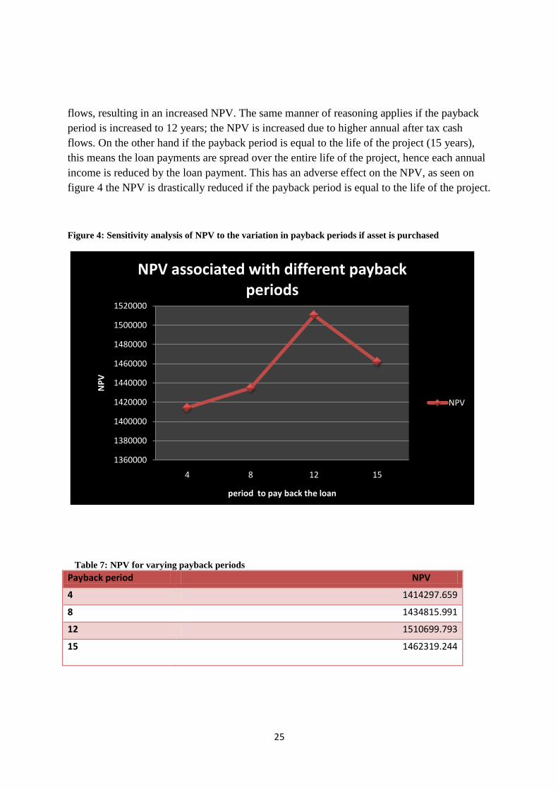
flows, resulting in an increased NPV. The same manner of reasoning applies if the payback
period is increased to 12 years; the NPV is increased due to higher annual after tax cash
flows. On the other hand if the payback period is equal to the life of the project (15 years),
this means the loan payments are spread over the entire life of the project, hence each annual
income is reduced by the loan payment. This has an adverse effect on the NPV, as seen on
figure 4 the NPV is drastically reduced if the payback period is equal to the life of the project.
Figure 4: Sensitivity analysis of NPV to the variation in payback periods if asset is purchased
Table 7: NPV for varying payback periods Payback period NPV
4 1414297.659
8 1434815.991
12 1510699.793
15 1462319.244
1360000
1380000
1400000
1420000
1440000
1460000
1480000
1500000
1520000
4 8 12 15
NP
V
period to pay back the loan
NPV associated with different payback periods
NPV

26
Figure 5 below illustrates how inflation affects the NPV associated with purchasing
calculations. The spreadsheets that support the information presented in figure 5 are
presented in appendix D. Inflation is the annual increase in the amount of money required to
purchase the same amount of goods. If the inflation rate is incorporated into the spreadsheet
model that represents purchasing, this results in the operating expenses increasing yearly at
the rate of inflation. As the inflation rate increases from 5% to 6.6% to 9.6% the NPV value
decreases since the yearly operating expenses also increases. The current inflation in South
Africa at the moment is estimated to be 6.6%, this estimate was determined through a process
called inflation targeting (de Jager & Kahan, 2011).
Figure 5: Sensitivity analysis of NPV to the variation in inflation if the asset is purchased
Table 8: NPV and inflation rates when purchasing
NPV inflation rate
1016691.3 5%
795365.58 6.60%
447344.19 9.60%
Further analysis was also done on the leasing spreadsheet. To investigate the effect of
inflation on the NPV if an asset is leased multiple leasing spreadsheets were prepared with
varying inflation rates. These spreadsheets can be seen in appendix E. Figure 6 below
0
200000
400000
600000
800000
1000000
1200000
5% 6.60% 9.60%
NP
V
Inflation rate
Change in NPV as inflation changes
NPV

27
demonstrates the results. The change in the inflation rate affects only the operating expenses
if the asset was leased. The lease payment expense is not affected because these payments are
determined at the beginning of the lease period and cannot be adjusted for inflation during the
duration of the lease; the inflation rate is considered when the payments are first established
at the beginning of the lease period. In figure 6, as the inflation rate increases from 5%, to
6.6% and to 9.6% the NPV of the leasing spread sheet is decreasing, the reason for this is that
as inflation gets higher the operating expenses get even more expensive. Once the inflation
hits 9.6%, the NPV will be negative, which makes the leasing option unacceptable. If the
inflation rate were to actually rise to 9.6% the asset would not be leased since the NPV when
the asset is leased is negative, the asset would be purchased because as seen in figure 5 the
NPV is positive when the asset is purchased and the inflation rate is 9.6%.
Figure 6: Sensitivity analysis of NPV to the variation in inflation rates if asset is leased
Table 9: NPV associated with different inflation rates when leasing
Inflation NPV
5% 313449.1171
6.60% 149529.2973
9.60% -305128.07
-400000
-300000
-200000
-100000
0
100000
200000
300000
400000
5% 6.60% 9.60%
NP
V
Inflation rate
Change in NPV as inflation changes
NPV

28
Figure 8 shows how different project lives can affect the NPV if an asset is leased. The
relevant spreadsheets are in Appendix F. As the life of the project is decreased from 12 to 9
years the NPV is also decreasing. The reason is that when the project life gets shorter, there
are less operating years hence, less income. When the asset is leased the market value of the
asset at the end of the project duration does not affect the NPV of profit from the project.
Figure 7: Sensitivity analysis of NPV to the variation in project life if the asset is leased
Table 10: NPV for different project durations in the leasing option
Project life Net Present Value
3 129421.4442
6 233247.6083
9 359744.6624
12 364691.2973
0
50000
100000
150000
200000
250000
300000
350000
400000
3 6 9 12
Ne
t P
rese
nt
Val
ue
Project Life
Change in NPV as project life increases
Net Present Value

29
To investigate how an increase in the interest rates would affect the profit expected from a
project whether the asset is leased or purchased further analysis was done on the leasing and
purchasing spreadsheet models and the results are show on figure 8 and figure 9. The
spreadsheet models supporting these graphs are on appendix G and appendix H respectively.
Figure 8: Sensitivity analysis of the affect of interest rate on the NPV an asset is purchased
Table 11: NPV for different interest rates
Interest rate NPV
0.07 1414270.194
0.08 1410565.397
0.11 1399170.018
0.14 1387507.857
1370000
1375000
1380000
1385000
1390000
1395000
1400000
1405000
1410000
1415000
1420000
0.07 0.08 0.11 0.14
NP
V
Interest rate
Change in NPV as interest rates increase
npv

30
Figure 9: Sensitivity analysis of the affect of interest rate on the NPV an asset is leased
Table 12: NPV and different interest rates when the asset is leased
INTERST RATE NPV
7% 364691.2973
8% 267922.9641
11% 231634.5301
14% 178398.398
From figure 8 and 9 it is evident that when the interest rate increases the return that is
expected on a project decreases, whether the asset was leased or purchased. However the
slope of the graph on figure 8 is –R 382 466.44 and the slope of the graph in figure 9 is
-R 3.7041E-07, these values show that an increase in the interest rates will have a higher
effect on the profit of a project if the assets used on the project are purchased.
0
50000
100000
150000
200000
250000
300000
350000
400000
7% 8% 11% 14%
NP
V
interest rates
Change in NPV as interest rate increases
npv

31
Chapter 5: Conclusions Based on the analysis in chapter 4, certain conclusions can be made regarding the effect that
inflation, interest rates and project life has on the decision to lease or purchase equipment.
The analysis also gave further insight on the effect of the loan payback period and the
percentage of equity used to purchase the equipment on the NPV if the asset is purchased.
The sensitivity analysis in figure 5 and 6 demonstrates the effect of different inflation
rates on the NPV when an asset is purchased and leased, respectively. The slope of
the graph in figure 5 is –12 277 451 and the slope of the graph in figure 6 is
-13 666 561, since figure 6 has a greater slope than figure 5 this implies that inflation
has a greater effect on the NPV if the asset is leased than when the asset is purchased.
Therefore, when an increase in inflation rate is expected it would be best to purchase
than to lease the asset.
The sensitivity analysis in figure 3 and in figure 7 show how the duration of the
project affects the NPV if the asset is purchased and leased respectively. The graph in
figure 3 has a slope of 37 551.576 and the slope of the graph in figure 7 is 27
743.55378. The slope of the sensitivity analysis graph (37 551.576) that reflects the
effect of the project life on the NPV when the asset is purchased is higher than the
slope of the sensitivity analysis graph (27 743.5) that shows the effect of the project
life when the asset leased. Therefore it can be concluded that it is best to lease the
asset than to purchase if the project life of the asset is less than 15 years.
Figure 8 demonstrates that as the interest rate increases the profit expected on a
project decreases at a rate of -382466 if the asset is purchased. On the other hand
figure 9 shows that as the interest rate increases the profit expected if the asset is
leased will decrease at a rate of -3.041E-07. From this it can be concluded that if a
rise in interest rates is anticipated it is best to lease the equipment.
If the decision to purchase the asset has been made the following conclusions can be made
based on figure 2 and 4.
Figure 2 shows the effect of using different values of own equity to purchase an asset
on the NPV when the asset is purchased. From this graph it can be concluded that it is
best to use a loan to purchase equipment since the return or profit of a project
decreases if own equity if used to finance the purchase price.
Figure 4 illustrates how different payback periods affect the NPV. Based on this
graph it can be concluded that as the loan payback period in increased the NPV will
also increase however, if the payback period is equal to the project life this leads to a
decrease in the NPV.

32
APPENDIX A – Purchasing models with different equity
Scenario: Purchase equipment using 25% equity.
Input table
Purchase price + VAT 254 218.86
Own equity 63 554.72
Loan Amount 190 664.15
Interest on loan (i) 7.00%
Payback period 4
Normal tax rate 28%
Secondary tax 10%
Life of project 15 years
Tax life 3 years
Year
CFBT
Depreciation
Book
Value
Loan
Interest
Operating cost
and maintenance
Taxable
Income
Loan
Payment
Tax
payment
CFAT
0 -63,554.72 -63,554.72
1 499200 -71072.9533 183,145.91 13346.53 179656 235124.516 56289.77553 65834.86 197419.36
2 499200 -71072.9533 112,072.95 10340.49 179656 238130.559 56289.77553 66676.56 196577.668
3 499200 -71072.9533 41,000.00 7124.034 229656 191347.013 56289.77553 53577.16 159677.061
4 499200 3682.59 179656 315861.41 56289.77553 88441.19 174813.03
5 499200 179656 319544 89472.32 230071.68
6 499200 229656 269544 75472.32 194071.68
7 499200 179656 319544 89472.32 230071.68
8 499200 179656 319544 89472.32 230071.68
9 499200 229656 269544 75472.32 194071.68
10 499200 179656 319544 89472.32 230071.68
11 499200 179656 319544 89472.32 230071.68
12 499200 229656 269544 75472.32 194071.68
13 499200 179656 319544 89472.32 230071.68
14 499200 179656 319544 89472.32 230071.68
15 499200 229656 269544 75472.32 194071.68
MV 58,157.12 41,000.00 17,157.12 4803.994 53,353.13
NPV:
-63 554.72 + 197 419.36(P/F,11,1) + 196 577.668(P/F,11,2) + 159 677.061(P/F,11,3) + 174 813.03(P/F,11,4)
230 071.68(P/F,11,5) + 194 071.68(P/F,11,6) + 230 071.68(P/A,11,2)(P/F,11,6) + 194 071.68(P/F,11,9)
230 071.68(P/,11,2)(F/P,11,9)+ 194 071.68(P/F,11,12) + 230 071.68(P/A,11,2)(P/F,11,12) + 194 071(P/F,11,15)
+ 53 353.13(P/F,11,15)
1406335.857

33
Scenario: Purchase equipment using 50% equity.
Input table
Purchase price + VAT 254 218.86
Own equity 63 554.72
Loan Amount 190 664.15
Interest on loan (i) 7.00%
Payback period 4
Normal tax rate 28%
Secondary tax 10%
Life of project 15 years
Tax life 3 years
Year
CFBT
Depreciation
Book
Value
Loan
Interest
Operating cost
and maintenance
Taxable
Income
Loan
Payment
Tax
payment
CFAT
0 -127,109.43 -127,109.43
1 499200 71072.95333 183,145.91 8923.956 179656 239547.091 37526.52 67073.19 214944.298
2 499200 71072.95333 112,072.95 6893.659 179656 241577.388 37526.52 67641.67 214375.814
3 499200 71072.95333 41,000.00 4749.356 R 229,656 193721.691 37526.52 54242.07 177775.41
4 499200 2455.06 179656 317088.94 37526.52 88784.9 193232.58
5 499200 179656 319544 89472.32 230071.68
6 499200 R 229,656 R 269,544 75472.32 194071.68
7 499200 179656 319544 89472.32 230071.68
8 499200 179656 319544 89472.32 230071.68
9 499200 R 229,656 269544 75472.32 194071.68
10 499200 179656 319544 89472.32 230071.68
11 499200 179656 319544 89472.32 230071.68
12 499200 R 229,656 269544 75472.32 194071.68
13 499200 179656 319544 89472.32 230071.68
14 499200 179656 319544 89472.32 230071.68
15 499200 R 229,656 269544 75472.32 194071.68
MV 58,157.12 41,000.00 17,157.12 4803.994 53,353.13
NPV:
-127 109.43 + 214 944(P/F,11,1) + 214 375.814(P/F,11,2) + 177 775.41(P/F,11,3) + 193 232.58(P/F,11,4)
230071.68(P/F,11,5) + 194 071.68(P/F,11,6) + 230 071.68(P/A,11,2)(P/F,11,6) + 194 071.68(P/F,11,9)
230 071.68(P/A,11,2)(P/F,11,9) + 194 071.68(P/F,11,12) + 194 071.68(P/F,11,12) + 230 071.68(P/A,11,2)(P/F,11,12)
194 071.68(P/F,11,15) + 53 353.13(P/F,11,15)
1398380.508

34
Scenario: Purchase equipment using 75% equity.
Input table
Purchase price + VAT 254 218.86
Own equity 63 554.72
Loan Amount 190 664.15
Interest on loan (i) 7.00%
Payback period 4
Normal tax rate 28%
Secondary tax 10%
Life of project 15 years
Tax life 3 years
Year
CFBT
Depreciation
Book
Value
Loan
Interest
Operating
cost
and
maintenance
Taxable
Income
Loan
Payment
Tax
payment
CFAT
0 -190,664.15 -190,664.15
1 499200 71,072.95 183,145.91 4448.8436 179656 244,022.20 18763.25851 68326.2168 232,454.52
2 499200 71,072.95 112,072.95 3446.8294 179656 245,024.22 18763.25851 68606.7808 232,173.96
3 499200 71,072.95 41,000.00 2374.678 229656 196,096.37 18763.25851 54906.9832 195,873.76
4 499200 1227.5299 179656 318,316.47 18763.25851 89128.6116 211,652.13
5 499200 179656 319,544.00 89472.32 230,071.68
6 499200 229656 269,544.00 75472.32 194,071.68
7 499200 179656 319,544.00 89472.32 230,071.68
8 499200 179656 319,544.00 89472.32 230,071.68
9 499200 229656 269,544.00 75472.32 194,071.68
10 499200 179656 319,544.00 89472.32 230,071.68
11 499200 179656 319,544.00 89472.32 230,071.68
12 499200 229656 269,544.00 75472.32 194,071.68
13 499200 179656 319,544.00 89472.32 230,071.68
14 499200 179656 319,544.00 89472.32 230,071.68
15 499200 229656 269,544.00 75472.32 194,071.68
MV 58157.12 41,000.00 17,157.12 4803.9936 53,353.13
NPV:
-190 664.15 + 232 454.52(P/F,11,1) + 232 173.96(P/F,11,2) + 195 873.76(P/F,11,3) + 211 652.13(P/F,11,4)
+ 230 071.68(P/F,11,5) + 194 071.68(P/F,11,6) + 230 071.68(P/A,11,2)(P/F,11,6) + 194 071.68(P/A,11,9)
+ 230 071.68(P/A,11,2)(P/F,11,9) + 194 071.68(P/F,11,12) + 230 071.68(P/A,11,2)(P/F,11,12)
+ 194 071.68(P/A,11,15) + 53 3553.13(P/A,11,15)
1390412.58

35
Scenario: Purchase equipment using 100% equity.
Input table
Purchase price +
VAT
254 218.86
Own equity (100%) 254 218.86
Loan Amount 0.00
Normal tax rate 28%
Secondary tax 10%
Life of project 15 years
Tax life 3 years
Year
CFBT
Depreciation
Book
Value
Operating cost
and maintenance
Taxable
Income
Tax
payment
CFAT
0 -254,218.86 -254,218.86
1 499200 71072.95333 183,145.91 179656 248471.047 69571.89307 249972.107
2 499200 71072.95333 112,072.95 179656 248471.047 69571.89307 249972.107
3 499200 71072.95333 41,000.00 229656 198471.047 55571.89307 213972.107
4 499200 179656 319544 89472.32 230071.68
5 499200 179656 319544 89472.32 230071.68
6 499200 229656 269544 75472.32 194071.68
7 499200 179656 319544 89472.32 230071.68
8 499200 179656 319544 89472.32 230071.68
9 499200 229656 269544 75472.32 194071.68
10 499200 179656 319544 89472.32 230071.68
11 499200 179656 319544 89472.32 230071.68
12 499200 229656 269544 75472.32 194071.68
13 499200 179656 319544 89472.32 230071.68
14 499200 179656 319544 89472.32 230071.68
15 499200 229656 269544 75472.32 194071.68
MV 58,157.12 41,000.00 17,157.12 4803.9936 53,353.13
NPV:
-254 218.86 + 249972.107(P/A,11,2) + 213972.107(P/F,11,3) + 230071.68(P/A,11,2)(P/F,11,3)
+ 194071.68(P/F,11,6) + 230071.68(P/A,11,2)(P/F,11,6) + 194071.68(P/F,11,9) + 230071.68(P/A,11,2)(P/F,11,9)
+ 194071.61(P/F,11,12) + 230071.68(P/A,11,2)(P/F,11,12) + 194071.68(P/F,11,15)
+ 53353.13(P/F,11,15)
1382446.222

36
APPENDIX B – Purchasing models with varying project life
Scenario: Purchase equipment using a loan.
Input table
Purchase price + VAT 254 218.86
Loan Amount 254 218.86
Interest on loan (i) 7.00%
Payback period 4
Normal tax rate 28%
Secondary tax 10%
Life of project 12 years
Tax life 3 years
Year
CFBT
Depreciation
Book
Value
Loan
Interest
Operating
cost
and
maintenance
Taxable
Income
Loan
Payment
Tax
payment
CFAT
0
1 499200 71072.95333 183,145.91 17795.37 179656 230675.67 75,053.03 64589.19 179901.78
2 499200 71072.95333 112,072.95 13787.32 179656 234683.73 75,053.03 65711.44 178779.52
3 499200 71072.95333 41,000.00 9498.71 229656 188972.33 75,053.03 52912.25 141578.71
4 499200 4910.12 179656 314633.88 75,053.03 88097.49 156393.48
5 499200 179656 319544.00 89472.32 230071.68
6 499200 229656 269544.00 75472.32 194071.68
7 499200 179656 319544.00 89472.32 230071.68
8 499200 179656 319544.00 89472.32 230071.68
9 499200 229656 269544.00 75472.32 194071.68
10 499200 179656 319544.00 89472.32 230071.68
11 499200 179656 319544.00 89472.32 230071.68
12 499200 229656 269544.00 75472.32 194071.68
MV 79776.572 41,000.00 38,776.57 10857.44 68,919.13
NPV:
179901.78(P/F,11,1) + 178 779.52(P/F,11,2) + 141 578.71(P/F,11,3) + 156 393.48(P/F,11,4) + 230 071.68(P/F,11,5)
194 071.68(P/F,11,6) + 230 0071.68(P/A,11,2)(P/F,11,6) + 194 071.68(P/F,11,9) + 230071.68(P/A,11,2)(P/F,11,9)
+ 194 071.68(P/F,11,12)+ 68 919.13(P/F,11,12)
1179742.95

37
Scenario: Purchase equipment using a loan.
Input table
Purchase price + VAT 254 218.86
Loan Amount 254 218.86
Interest on loan (i) 7.00%
Payback period 4
Normal tax rate 28%
Secondary tax 10%
Life of project 9 years
Tax life 10 years
Year
CFBT
Depreciation
Book
Value
Loan
Interest
Operating cost
and maintenance
Taxable
Income
Loan
Payment
Tax
payment
CFAT
0
1 499200 71072.95333 183,145.91 17795.37 179656 230675.67 75,053.03 64589.19 179901.78
2 499200 71072.95333 112,072.95 13787.32 179656 234683.73 75,053.03 65711.44 178779.52
3 499200 71072.95333 41,000.00 9498.71 179656 238972.33 75,053.03 66912.25 177578.71
4 499200 4910.12 179656 314633.88 75,053.03 88097.49 156393.48
5 499200 179656 319544.00 89472.32 230071.68
6 499200 179656 319544.00 89472.32 230071.68
7 499200 179656 319544.00 89472.32 230071.68
8 499200 179656 319544.00 89472.32 230071.68
9 499200 179656 319544.00 89472.32 230071.68
MV 109432.9 41,000.00 68,432.88 19161.21 90271.68
NPV:
179 901.78(P/F,11,1) + 178 779.52(P/F,11,2) + 177 578.71(P/F,11,3) + 156 393.48(P/F,11,4) +
230071.68(P/A,11,5)(P/F,11,4) + 90 271.68(P/F,11,9)
1141355.46
38
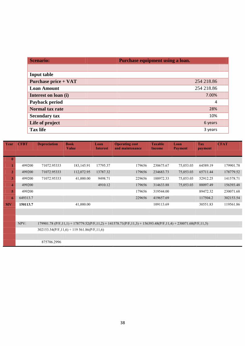
Scenario: Purchase equipment using a loan.
Input table
Purchase price + VAT 254 218.86
Loan Amount 254 218.86
Interest on loan (i) 7.00%
Payback period 4
Normal tax rate 28%
Secondary tax 10%
Life of project 6 years
Tax life 3 years
Year
CFBT
Depreciation
Book
Value
Loan
Interest
Operating cost
and maintenance
Taxable
Income
Loan
Payment
Tax
payment
CFAT
0
1 499200 71072.95333 183,145.91 17795.37 179656 230675.67 75,053.03 64589.19 179901.78
2 499200 71072.95333 112,072.95 13787.32 179656 234683.73 75,053.03 65711.44 178779.52
3 499200 71072.95333 41,000.00 9498.71 229656 188972.33 75,053.03 52912.25 141578.71
4 499200 4910.12 179656 314633.88 75,053.03 88097.49 156393.48
5 499200 179656 319544.00 89472.32 230071.68
6 649313.7 229656 419657.69 117504.2 302153.54
MV 150113.7 41,000.00 109113.69 30551.83 119561.86
NPV: 179901.78 (P/F,11,1) + 178779.52(P/F,11,2) + 141578.71(P/F,11,3) + 156393.48(P/F,11,4) + 230071.68(P/F,11,5)
302153.54(P/F,11,6) + 119 561.86(P/F,11,6)
875706.2996

39
Scenario: Purchase equipment using a loan.
Input table
Purchase price + VAT 254 218.86
Loan Amount 254 218.86
Interest on loan (i) 7.00%
Payback period 4
Normal tax rate 28%
Secondary tax 10%
Life of project 3 years
Tax life 3 years
Year
CFBT
Depreciation
Book
Value
Loan
Interest
Operating cost
and maintenance
Taxable
Income
Loan
Payment
Tax
payment
CFAT
0
1 499200 71072.95 183,145.91 17795.37 179656 410331.67 75,053.03 114,892.87 309254.10
2 499200 71072.95 112,072.95 13787.32 179656 414339.73 75,053.03 116,015.12 308131.84
3 705117.277 71072.95 41,000.00 9498.71 R 229,656 624545.61 75,053.03 174,872.77 455191.47
4 4910.12 75,053.03 -75053.03
NPV: 309254.10 (P/F,11,1) + 308131.84(P/F,11,2) + 455 191.47(P/F,11,3) - 75053.03(P/F,11,4)
812085.39

40
APPENDIX C- Purchasing models with different pay back periods
Scenario: Purchase equipment using a loan.
Input table
Purchase price + VAT 254 218.86
Loan Amount 254 218.86
Interest on loan (i) 7.00%
Payback period 8 years
Normal tax rate 28%
Secondary tax 10%
Life of project 15 years
Tax life 3 years
Year
CFBT
Depreciation
Book Value
Loan Interest
Operating cost and maintenance
Taxable Income
Loan Payment
Tax payment
CFAT
0
1 499200 71072.95333 183,145.91 17795.56 179656 230675.48 42,574.03 64589.14 212380.83
2 499200 71072.95333 112,072.95 16061.10 179656 232409.95 42,574.03 65074.79 211895.18
3 499200 71072.95333 41,000.00 14205.04 229656 184266.01 42,574.03 51594.48 175375.49
4 499200 12219.34 179656 307324.66 42,574.03 86050.9 190919.06
5 499200 10094.47 179656 309449.53 42,574.03 86645.87 190324.10
6 499200 7820.89 229656 261723.11 42,574.03 73282.47 153687.50
7 499200 5388.17 179656 314155.83 42,574.03 87963.63 189006.33
8 499200 2785.28 179656 316758.72 42,574.03 88692.44 188277.53
9 499200 229656 269544.00 75472.32 194071.68
10 499200 179656 319544.00 89472.32 230071.68
11 499200 179656 319544.00 89472.32 230071.68
12 499200 229656 269544.00 75472.32 194071.68
13 499200 179656 319544.00 89472.32 230071.68
14 499200 179656 319544.00 89472.32 230071.68
15 499200 229656 269544.00 75472.32 194071.68
MV 58157.121 41,000.00 17,157.12 4803.994 53353.13
NPV:
212 380.83(P/F,11,1) + 211 895.18(P/F,11,2) + 175 375.49(P/F,11,3) + 190 919.06(P/F,11,4) + 190 324.10*(F/P,11,5) +
153 687.50(P/F,11,6) + 189 006.33(P/F,11,7) + 188 277.53(P/F,11,8) + 194 071.68(P/F,11,9) + 230 071.68(P/A,11,2)(P/F,11,9)
+ 194 071.68(P/F,11,12) + 230 071.68(P/A,11,2)(P/F,11,12) + 194 071.68(P/F,11,15)
+ 53353.13(P/F,11,15)
1434815.991

41
Scenario: Purchase equipment using a loan.
Input table
Purchase price + VAT 254 218.86
Loan Amount 254 218.86
Interest on loan (i) 7.00%
Payback period 12 years
Normal tax rate 28%
Secondary tax 10%
Life of project 15 years
Tax life 3 years
Year
CFBT
Depreciation
Book
Value
Loan
Interest
Operating cost
and maintenance
Taxable
Income
Loan
Payment
Tax
payment
CFAT
0
1 499200 71072.95333 183,145.91 15778.68 179656 232692.36 32,006.15 65153.86 222383.98
2 499200 71072.95333 112,072.95 16800.32 179656 231670.73 32,006.15 64867.8 222670.04
3 499200 71072.95333 41,000.00 15735.89 229656 182735.16 32,006.15 51165.84 186372.00
4 499200 14596.85 179656 304947.15 32,006.15 85385.2 202152.64
5 499200 13378.28 179656 306165.72 32,006.15 85726.4 201811.45
6 499200 12074.35 229656 257469.65 32,006.15 72091.5 165446.34
7 499200 10679.01 179656 308864.99 32,006.15 86482.2 201055.65
8 499200 9186.21 179656 310357.79 32,006.15 86900.18 200637.67
9 499200 7588.79 229656 261955.21 32,006.15 73347.46 164190.39
10 499200 5879.56 179656 313664.44 32,006.15 87826.04 199711.80
11 499200 4050.70 179656 315493.30 32,006.15 88338.12 199199.72
12 499200 2093.91 229656 267450.09 32,006.15 74886.03 162651.82
13 499200 179656 319544.00 319544.00
14 499200 179656 319544.00 319544.00
15 499200 229656 269544.00 269544.00
MV 58157.12 41,000.00 17,157.12 4803.994 53353.13
NPV:
222 238.98 (P/F,11,1)+ 222 670.04(P/F,11,2) + 186 372.00(P/F,11,3) + 202152.64(P/F,11,4) +
201 811.45(P/F,11,5)+165 446.34(P/F,11,6) + 201 055.65(P/F,11,7) + 200 637.67P/F,11,8) + 164 190.39(P/F,11,9)
+199 199.80(P/F,11,10)+ 199 199.72(P/F,11,11) + 162 651.82(P/F,11,12) +319 544(P/A,11,2)(P/F,11,12)
+ 269 544(P/F,11,15) + 53353.13(P/F,11,15)
1510699.793

42
Scenario: Purchase equipment using a loan.
Input table
Purchase price + VAT 254 218.86
Loan Amount 254 218.86
Interest on loan (i) 7.00%
Payback period 4
Normal tax rate 28%
Secondary tax 10%
Life of project 15 years
Tax life 3 years
Year
CFBT
Depreciation
Book
Value
Loan
Interest
Operating cost
and maintenance
Taxable
Income
Loan
Payment
Tax
payment
CFAT
0
1 499200 71072.95333 183,145.91 17794.54 179656 230676.50 27,910.69 64589.42 227043.89
2 499200 71072.95333 112,072.95 17086.50 179656 231384.54 27,910.69 64787.67 226845.64
3 499200 71072.95333 41,000.00 16757.30 229656 181713.75 27,910.69 50879.85 190753.46
4 499200 15518.04 179656 304025.96 27,910.69 85127.27 206506.04
5 499200 14650.57 179656 304893.43 27,910.69 85370.16 206263.15
6 499200 13722.35 229656 255821.65 27,910.69 71630.06 170003.25
7 499200 12729.06 179656 306814.94 27,910.69 85908.18 205725.13
8 499200 11666.42 179656 307877.58 27,910.69 86205.72 205427.59
9 499200 10529.34 229656 259014.66 27,910.69 72524.11 169109.21
10 499200 9312.54 179656 310231.46 27,910.69 86864.81 204768.50
11 499200 8010.76 179656 311533.24 27,910.69 87229.31 204404.00
12 499200 6422.36 229656 263121.64 27,910.69 73674.06 167959.25
13 499200 5163.76 179656 314380.24 27,910.69 88026.47 203606.84
14 499200 3532.38 179656 316011.62 27,910.69 88483.25 203150.06
15 499200 1825.97 229656 267718.03 27,910.69 74961.05 166672.26
MV 58157.12 41,000.00 17,157.12 4803.994 53,353.13
NPV:
227 093.12(P/F,11,1) + 226 845.64(P/F,11,2) + 190 753.46(P/F,11,3) + 206 506.04(P/F,11,4) + 206 263.15(P/F,11,5) +
170003.25(P/F,11,6) + 205725.13(P/F,11,7) + 205 527.59(P/F,11,8)+ 169 109.21(P/F,11,9) + 204 768.50(P/F,11,10) +
204 404.00(P/F,11,11)+167 959.25(P/F,11,12) + 203 606.84(P/F,11,13) + 203 150.06(P/F,11,14) + 166 672.26(P/F,11,15)
+ 53 353.13(P/F,11,15)
1462319

43
APPENDIX D-Purchasing models with different inflation rates
Scenario: Purchase equipment using a loan.
Input table
Purchase price + VAT 254 218.86
Loan Amount 254 218.86
Interest on loan (i) 7.00%
Payback period 4
Normal tax rate 28%
Secondary tax 10%
Life of project 15 years
Tax life 3 years
Inflation rate 9.60%
Year
CFBT
Depreciation
Book
Value
Loan
Interest
Operating cost
and maintenance
Taxable
Income
Loan
Payment
Tax
payment
CFAT
0
1 499200 71072.95 183 145.91 17795.37 179656 230675.67 75 053.03 64 589.19 179901.78
2 499200 71072.95 112 072.95 13787.32 179656 234683.73 75 053.03 65 711.44 178779.52
3 499200 71072.95 41 000.00 9498.71 R 229 656 188972.33 75 053.03 52 912.25 141578.71
4 499200 4910.12 179656 314633.88 75 053.03 88 097.49 156393.48
5 499200 179656 319544.00 89 472.32 230 071.68
6 499200 R 229 656 269544.00 75 472.32 194 071.68
7 499200 179656 319544.00 89 472.32 230 071.68
8 499200 179656 319544.00 89 472.32 230 071.68
9 499200 R 229 656 269544.00 75 472.32 194 071.68
10 499200 179656 319544.00 89 472.32 230 071.68
11 499200 179656 319544.00 89 472.32 230 071.68
12 499200 R 229 656 269544.00 75 472.32 194 071.68
13 499200 179656 319544.00 89 472.32 230 071.68
14 499200 179656 319544.00 89 472.32 230 071.68
15 499200 R 229 656 269544.00 75 472.32 194 071.68
MV 58 157 41 000.00 17 157.12 4 803.99 53 353.13
NPV :
179 901.78(P/F,11,1) + 178 779.52(P/F,11,2) + 141 578.71(P/F,11,3) + 156 393.48(P/F,11,4) + 230 071.68(P/F,11,5)
194 071.68(P/F,11,6) + 230 071.68(P/A,11,2)(P/F,11,6) + 194 071.68(P/F,11,9) + 230 071.68(P/A,11,2)(P/F,11,9)
+ 194 071.68(P/F,11,12) + 230 071.68(P/A,11,2)(P/F,11,12) + 194(P/F,11,15) + 53 353.13(P/F,11,15)
1223341

44
Scenario: Purchase equipment using a loan.
Input table
Purchase price + VAT 254 218.86
Loan Amount 254 218.86
Interest on loan (i) 7.00%
Payback period 4
Normal tax rate 28%
Secondary tax 10%
Life of project 15 years
Tax life 3 years
Inflation rate 6.60%
Year
CFBT
Depreciation
Book
Value
Loan
Interest
Operating cost
and maintenance
Taxable
Income
Loan
Payment
Tax
payment
CFAT
0
1 499200 -71072.95 183 145.91 17795.37 196902.976 213428.70 75 053.03 59 760.03 167483.96
2 499200 -71072.95 112 072.95 13787.32 215805.6617 198534.07 75 053.03 55 589.54 152751.77
3 499200 -71072.95 41 000.00 9498.71 R 302 350 116278.69 75 053.03 32 558.03 89239.29
4 499200 4910.12 259229.2137 235060.67 75 053.03 65 816.99 99100.77
5 499200 284115.2182 215084.78 60 223.74 154861.04
6 499200 R 398 053 101146.80 28 321.10 72825.69
7 499200 341283.746 157916.25 44 216.55 113699.70
8 499200 374046.9856 125153.01 35 042.84 90110.17
9 499200 R 524 050 -24850.07 -24850.07
10 499200 449311.2239 49888.78 13 968.86 35919.92
11 499200 492445.1014 6754.90 1 891.37 4863.53
12 499200 R 689 929 -190729.07 -190729.07
13 499200 591532.9349 -92332.93 -92332.93
14 499200 648320.0966 -149120.10 -149120.10
15 499200 R 908 314 -409114.21 -409114.21
MV 58 157 41 000.00 17 157.12 4 803.99 R 53 353.13
NPV when taking in to account the inflation rate (6.6%):
167 483.96(P/F,11,1)+ 152 751.77(P/F,11,2)+ 89239.29(P/F,11,3) + 99 100.77(P/F,11,4) + 154 861.04(P/F,11,5) + 72 825.69(P/F,11,6)+
113 699.70(P/F,11,7) + 90 110.17(P/F,11,8) - 24 850.07(P/F,11,9) + 35 919.92(P/F,11,10) + 4863.53(P/F,11,11) - 190 729.07(P/F,11,12)+
-92 332(P/F,11,13) - 149 120.10(P/F,11,14) - 409 114.21(P/F,11,15) + 53 353.13(P/F,11,15)
447344.19

45
Scenario: Purchase equipment using a loan.
Input table
Purchase price + VAT 254 218.86
Loan Amount 254 218.86
Interest on loan (i) 7.00%
Payback period 4
Normal tax rate 28%
Secondary tax 10%
Life of project 15 years
Tax life 3 years
Inflation rate 5.0%
Year
CFBT
Depreciation
Book
Value
Loan
Interest
Operating
cost
and
maintenance
Taxable
Income
Loan
Payment
Tax
payment
CFAT
0
1 499200 -71072.95 183 145.91 17795.37 188638.8 221692.87 75 053.03 62 074.00 173434.16
2 499200 -71072.95 112 072.95 13787.32 198070.74 216268.99 75 053.03 60 555.32 165520.91
3 499200 -71072.95 41 000.00 9498.71 R 265 856 152772.81 75 053.03 42 776.39 115515.05
4 499200 4910.12 218372.9909 275916.89 75 053.03 77 256.73 128517.25
5 499200 229291.6404 269908.36 75 574.34 194334.02
6 499200 R 325 771 173428.57 48 560.00 124868.57
7 499200 270136.1978 229063.80 64 137.86 164925.94
8 499200 265433.7352 233766.26 65 454.55 168311.71
9 499200 R 356 272 142928.17 40 019.89 102908.28
10 499200 292640.6931 206559.31 57 836.61 148722.70
11 499200 307272.7277 191927.27 53 739.64 138187.64
12 499200 R 412 429 86770.82 24 295.83 62474.99
13 499200 338768.1823 160431.82 44 920.91 115510.91
14 499200 355706.5914 143493.41 40 178.15 103315.25
15 499200 R 477 438 21761.67 6 093.27 15668.40
MV 58 157 41 000.00 17 157.12 4 803.99 R 53
353.13
NPV when taking in to account the inflation rate (5%):
1016691

46
APPENDIX E- Leasing models with different inflation rates
Scenario: Acquiring equipment through leasing
Input table
Purchase price +
VAT
254 218.86
Annual lease
payment
215 162.46
Normal tax rate 28%
Secondary tax 10%
Life of project 15 years
Tax life 3 years
Inflation rate 6.6%
Year
CFBT
lease payment
Operating cost
and maintenance
Taxable
Income
Tax
payment
CFAT
0
1 499200 430324.92 191513.296 -122638.216 -122638.216
2 499200 215162.46 204153.1735 79884.36646 22367.62 57516.74385
3 499200 215162.46 217627.283 66410.25701 18594.87 47815.38505
4 499200 215162.46 231990.6837 52046.85633 14573.12 37473.73656
5 499200 215162.46 247302.0688 36735.47121 10285.93 26449.53927
6 499200 215162.46 263624.0053 20413.53467 5715.79 14697.74496
7 499200 215162.46 281023.1897 3014.35032 844.0181 2170.33223
8 499200 215162.46 299570.7202 -15533.1802 -15533.1802
9 499200 215162.46 319342.3877 -35304.84773 -35304.84773
10 499200 215162.46 340418.9853 -56381.44532 -56381.44532
11 499200 215162.46 362886.6384 -78849.09835 -78849.09835
12 499200 386837.1565 112362.8435 31461.6 80901.24733
NPV:
- 110 780 (P/F,11,1)+ 75 154.709*(P/A,11,10) (P/F,11,1)+ 230 071.68*(P/F,11,12)
149529.2973

47
Scenario: Acquiring equipment through leasing
Input table
Purchase price +
VAT
254 218.86
Annual lease
payment
215 162.46
Normal tax rate 28%
Secondary tax 10%
Life of project 15 years
Tax life 3 years
Inflation rate 5%
Year CFBT lease payment Operating cost Taxable Tax CFAT
and maintenance Income payment
0
1 499200 430324.92 188638.8 -119763.72 -119763.72
2 499200 215162.46 198070.74 85966.8 24070.704 61896.096
3 499200 215162.46 207974.277 76063.263 21297.7136 54765.54936
4 499200 215162.46 218372.9909 65664.5492 18386.0738 47278.47539
5 499200 215162.46 229291.6404 54745.8996 15328.8519 39417.04772
6 499200 215162.46 240756.2224 43281.3176 12118.7689 31162.54866
7 499200 215162.46 252794.0335 31243.5065 8748.18181 22495.32466
8 499200 215162.46 265433.7352 18603.8048 5209.06534 13394.73945
9 499200 215162.46 278705.422 5332.11803 1492.99305 3839.124982
10 499200 215162.46 292640.6931 -8603.1531 -8603.153068
11 499200 215162.46 307272.7277 -23235.188 -23235.18772
12 499200 322636.3641 176563.636 49437.818 127125.8178
NPV:
- 119763.72 (P/F,11,1)+ 61896.096*(P/F,11,2)+ 54765.54936(P/F,11,3) + 47278.47539(P/F,11,4) + 39417.04772(P/F,11,5)
+ 31162.54866(P/F,11,6) + 22495.32466(P/F,11,7) + 13394.73945(P/F,11,8) + 3839.124982 (P/F,11,9)- 8603.153068(P/F,11,10) +
- 23235.18772(P/F,11,11) + 127125.8178(P/F,11,12)
313449.1171

48
Scenario: Acquiring equipment through leasing
Input table
Purchase price +
VAT
254 218.86
Annual lease
payment
215 162.46
Normal tax rate 28%
Secondary tax 10%
Life of project 15 years
Tax life 3 years
Inflation rate 9.6%
Year CFBT lease payment Operating cost Taxable Tax CFAT
and maintenance Income payment
0
1 499200 430324.92 196902.976 -128027.896 -128028
2 499200 215162.46 215805.6617 68231.8783 19104.92593 49126.95
3 499200 215162.46 236523.0052 47514.53478 13304.06974 34210.47
4 499200 215162.46 259229.2137 24808.32628 6946.331358 17861.99
5 499200 215162.46 284115.2182 -77.67823693 -77.6782
6 499200 215162.46 311390.2792 -27352.73919 -27352.7
7 499200 215162.46 341283.746 -57246.20599 -57246.2
8 499200 215162.46 374046.9856 -90009.4456 -90009.4
9 499200 215162.46 409955.4962 -125917.9562 -125918
10 499200 215162.46 449311.2239 -165273.6839 -165274
11 499200 215162.46 492445.1014 -208407.5614 -208408
12 499200 539719.8311 -40519.83108 -40519.8
NPV:
- 128028*(P/F,11,1)+ 49126*(P/F,11,2)+ 34210.47*(P/F,11,3)+ 17861.99*(P/F,11,4) - 77.6782*(P/F,11,5) -
27352.7*(P/F,11,6) - 57246.2*(P/F,11,7) - 90009.4*(P/F,11,8) - 125918(P/F,11,9) - 165274*(P/F,11,10) -
208408(P/F,11,11) - 40519.8*(P/F,11,12)
-305128.07

49
APPENDIX F- leasing models with varying project lives
Scenario: Acquiring equipment through leasing
Input table
Purchase price + VAT 254 218.86
Annual lease payment 215 162.46
Normal tax rate 28%
Secondary tax 10%
Life of project 9 years
Tax life 10 years
Year CFBT lease payment Operating cost Taxable Tax CFAT
and maintenance Income payment
0 -215162.46
1 499200 430324.92 179656 -110780.92 -110780.92
2 499200 215162.46 179656 104381.54 29226.83 75154.7088
3 499200 215162.46 179656 104381.54 29226.83 75154.7088
4 499200 215162.46 179656 104381.54 29226.83 75154.7088
5 499200 215162.46 179656 104381.54 29226.83 75154.7088
6 499200 215162.46 179656 104381.54 29226.83 75154.7088
7 499200 215162.46 179656 104381.54 29226.83 75154.7088
8 499200 215162.46 179656 104381.54 29226.83 75154.7088
9 499200 499200 139776 359424
NPV
-215 162 - 110 780.92(P/F,11,1) + 75 154.71*(P/A,11,7)(P/F,11,1) + 359 424*(P/F,11,9)
359744.6624

50
Scenario: Acquiring equipment through leasing
Input table
Purchase price + VAT 254 218.86
Annual lease payment 215 162.46
Normal tax rate 28%
Secondary tax 10%
Life of project 6 years
Tax life 10 years
Year CFBT lease payment Operating cost Taxable Tax CFAT
and maintenance Income payment
0 -215,162.46
1 499200 430,324.92 179656 -110,780.92 -110,780.92
2 499200 215,162.46 179656 104,381.54 29226.8312 75,154.71
3 499200 215,162.46 179656 104,381.54 29226.8312 75,154.71
4 499200 215,162.46 179656 104,381.54 29226.8312 75,154.71
5 499200 215,162.46 179656 104,381.54 29226.8312 75,154.71
6 499200 179656 319,544.00 89472.32 230,071.68
MV:
- 215 162.46 - 110780.92(P/A,11,1) + 75 154.71*(P/A,11,4)(P/F,11,1) + 230 071.68*(P/F,11,6)
233247.6083

51
Scenario: Acquiring equipment through leasing
Input table
Purchase price + VAT 254 218.86
Annual lease payment 215 162.46
Normal tax rate 28%
Secondary tax 10%
Life of project 3 years
Tax life 10 years
Life of equipment 15 years
Year CFBT lease payment Operating cost Taxable Tax CFAT
and maintenance Income payment
0 -215,162.46
1 499200 430,324.92 179656 -110,780.92 -110,780.92
2 499200 215,162.46 179656 104,381.54 29226.83 75,154.71
3 499200 179656 319,544.00 89472.32 230,071.68
NPV:
-215 162.46 - 110780.92(P/F,11,1) + 75 154.71*(P/F,11,2) + 230 071.68*(P/F,11,3)
129421.444

52
Appendix G – purchasing models with varying interest rates
Cash Flow Analysis for purchasing a hydraulic mixer using a loan.
Scenario: Purchase equipment using a loan.
Input table
Purchase price + VAT 254,218.86
Loan Amount 254,218.86
Interest on loan (i) 8.00%
Payback period 4
Normal tax rate 28%
Secondary tax 10%
Life of project 15 years
Tax life 3 years
Year
CFBT
Depreciation
Book
Value
Loan
Interest
Operating cost
and maintenance
Taxable
Income
Loan
Payment
Tax
payment
CFAT
0
1 499200 71072.95 183,145.91 20337.29 179656 228133.76 76,753.76 63877.45 178,912.79
2 499200 71072.95 112,072.95 15824.17 179656 232646.88 76,753.76 65141.13 177649.12
3 499200 71072.95 41,000.00 10950.00 R 229,656 187521.05 76,753.76 52505.89 140284.35
4 499200 5685.30 179656 313858.70 76,753.76 87880.43 154909.81
5 499200 179656 319544.00 89472.32 230071.68
6 499200 R 229,656 269544.00 75472.32 194071.68
7 499200 179656 319544.00 89472.32 230071.68
8 499200 179656 319544.00 89472.32 230071.68
9 499200 R 229,656 269544.00 75472.32 194071.68
10 499200 179656 319544.00 89472.32 230071.68
11 499200 179656 319544.00 89472.32 230071.68
12 499200 R 229,656 269544.00 75472.32 194071.68
13 499200 179656 319544.00 89472.32 230071.68
14 499200 179656 319544.00 89472.32 230071.68
15 499200 R 229,656 269544.00 75472.32 194071.68
MV 58157.121 41,000.00 17,157.12 4803.994 53,353.13
NPV
178912.79(P/F,11,1) + 177649.12(P/F,11,2) + 140284.35(P/F,11,3) + 154909.81(P/F,11,4) + 230071.68(P/F,11,5) + 194071.68(P/F,11,6)
230071.68(P/A,11,2)(P/F,11,6) + 194071.68(P/F,11,9) + 230071.68(P/A,11,2)(P/F,11,9) + 194071.68(P/F,11,12)
230071.68(P/A,11,2)(P/F,11,12) + 194071.68(P/F,11,15) + 53353.13(P/F,11,15)
1410565.397

53
Scenario: Purchase equipment using a loan.
Input table
Purchase price + VAT 254,218.86
Loan Amount 254,218.86
Interest on loan (i) 11.00%
Payback period 4
Normal tax rate 28%
Secondary tax 10%
Life of project 15 years
Tax life 3 years
Year CFBT Depreciation Book Loan Operating cost Taxable Loan Tax CFAT
Value Interest and maintenance Income Payment payment
0
1 499200 71072.95333 183,145.91 27963.98 179656 220507.07 81,942.37 61741.98 175859.66
2 499200 71072.95333 112,072.95 22026.68 179656 226444.37 81,942.37 63404.42 174197.21
3 499200 71072.95333 41,000.00 15435.89 R 229,656 183035.15 81,942.37 51249.84 136351.79
4 499200 8120.41 179656 311423.59 81,942.37 87198.61 150403.03
5 499200 179656 319544.00 89472.32 230071.68
6 499200 R 229,656 269544.00 75472.32 194071.68
7 499200 179656 319544.00 89472.32 230071.68
8 499200 179656 319544.00 89472.32 230071.68
9 499200 R 229,656 269544.00 75472.32 194071.68
10 499200 179656 319544.00 89472.32 230071.68
11 499200 179656 319544.00 89472.32 230071.68
12 499200 R 229,656 269544.00 75472.32 194071.68
13 499200 179656 319544.00 89472.32 230071.68
14 499200 179656 319544.00 89472.32 230071.68
15 499200 R 229,656 269544.00 75472.32 194071.68
MV 58157.121 41,000.00 17,157.12 4803.994 53,353.13
NPV
175859.66(P/F,11,1) + 174197.21(P/F,11,2) + 136351.79(P/F,11,3) + 150403.03(P/F,11,4) + 230071.68(P/F,11,5)
194071.68(P/F,11,6) + 230071.68(P/A,11,2)(P/F,11,6) + 194071.68(P/F,11,9) + 230071(P/A,11,2)(P/F,11,9)
194071.68(P/F,11,12) + 230071.68(P/A,11,2)(P/F,11,12) + 194071.68(P/F,11,15) + 53353.13(P/F,11,15)
1399170.02

54
Scenario: Purchase equipment using a loan.
Input table
Purchase price + VAT 254,218.86
Loan Amount 254,218.86
Interest on loan (i) 14.00%
Payback period 4
Normal tax rate 28%
Secondary tax 10%
Life of project 15 years
Tax life 3 years
Year
CFBT
Depreciation
Book
Value
Loan
Interest
Operating
cost
and
maintenance
Taxable
Income
Loan
Payment
Tax
payment
CFAT
0
1 499200 71072.95333 183,145.91 35589.99 179656 212881.05 87,247.91 59606.69473 172689.39
2 499200 71072.95333 112,072.95 28357.67 179656 220113.38 87,247.91 61631.7467 170664.34
3 499200 71072.95333 41,000.00 20113.96 R 229,656 178357.09 87,247.91 49939.98446 132356.10
4 499200 10714.74 179656 308829.26 87,247.91 86472.19233 145823.89
5 499200 179656 319544.00 89472.32 230071.68
6 499200 R 229,656 269544.00 75472.32 194071.68
7 499200 179656 319544.00 89472.32 230071.68
8 499200 179656 319544.00 89472.32 230071.68
9 499200 R 229,656 269544.00 75472.32 194071.68
10 499200 179656 319544.00 89472.32 230071.68
11 499200 179656 319544.00 89472.32 230071.68
12 499200 R 229,656 269544.00 75472.32 194071.68
13 499200 179656 319544.00 89472.32 230071.68
14 499200 179656 319544.00 89472.32 230071.68
15 499200 R 229,656 269544.00 75472.32 194071.68
MV 58157.12 41,000.00 17,157.12 4803.993875 53353.13
NPV
172689.39(P/F,11,1) + 170664.34(P/F,11,2) + 132356.10(P/F,11,3) + 145823.89(P/F,11,4) + 230071.68(P/F,11,5)
194071.68(P/F,11,6) + 230071.68(P/A,11,2)(P/F,11,6) + 194071.68(P/F,11,9) + 230071.68(P/A,11,2)(P/F,11,9)
194071.68(P/F,11,12) + 230071.68(P/A,11,2)(P/F,11,12) + 194071.68(P/F,11,15) + 53353.13(P/F,11,15)
1387507.857

55
Appendix H- leasing models with varying interest rates
Cash Flow Analysis
Scenario: Acquiring equipment through leasing
Input table
Purchase price + VAT 254,218.86
interest rate 8%
Annual lease payment 232,375.46
Normal tax rate 28%
Secondary tax 10%
Life of project 15 years
Tax life 3 years
Year
CFBT
lease payment
Operating cost
and maintenance
Taxable
Income
Tax
payment
CFAT
0
1 499200 464750.9136 179656 -145206.9136 -145206.914
2 499200 232375.4568 179656 87168.5432 24407.1921 62761.3511
3 499200 232375.4568 179656 87168.5432 24407.1921 62761.3511
4 499200 232375.4568 179656 87168.5432 24407.1921 62761.3511
5 499200 232375.4568 179656 87168.5432 24407.1921 62761.3511
6 499200 232375.4568 179656 87168.5432 24407.1921 62761.3511
7 499200 232375.4568 179656 87168.5432 24407.1921 62761.3511
8 499200 232375.4568 179656 87168.5432 24407.1921 62761.3511
9 499200 232375.4568 179656 87168.5432 24407.1921 62761.3511
10 499200 232375.4568 179656 87168.5432 24407.1921 62761.3511
11 499200 232375.4568 179656 87168.5432 24407.1921 62761.3511
12 499200 179656 319544 89472.32 230071.68
NPV
-145206.914(P/F,11,1)) + 62761.3511(P/A,11,10)(P/F,11,1) + 230071.68(P/F,11,12)
267923

56
Cash Flow Analysis
Scenario: Acquiring equipment through leasing
Input table
Purchase price + VAT 254,218.86
interest rate 11%
Annual lease payment 232,375.46
Normal tax rate 28%
Secondary tax 10%
Life of project 15 years
Tax life 3 years
Year
CFBT
lease payment
Operating cost
and maintenance
Taxable
Income
Tax
payment
CFAT
0
1 499200 477660.6612 179656 -158116.6612 -158117
2 499200 238830.3306 179656 80713.6694 22599.83 58113.84
3 499200 238830.3306 179656 80713.6694 22599.83 58113.84
4 499200 238830.3306 179656 80713.6694 22599.83 58113.84
5 499200 238830.3306 179656 80713.6694 22599.83 58113.84
6 499200 238830.3306 179656 80713.6694 22599.83 58113.84
7 499200 238830.3306 179656 80713.6694 22599.83 58113.84
8 499200 238830.3306 179656 80713.6694 22599.83 58113.84
9 499200 238830.3306 179656 80713.6694 22599.83 58113.84
10 499200 238830.3306 179656 80713.6694 22599.83 58113.84
11 499200 238830.3306 179656 80713.6694 22599.83 58113.84
12 499200 179656 319544 89472.32 230071.7
NPV
-158117 (P/F,11,1) + 58113.84(P/A,11,10) (P/F,11,1) + 230071.7(P/F,11,12)
231634.5301

57
Cash Flow Analysis
Scenario: Acquiring equipment through leasing
Input table
Purchase price + VAT 254,218.86
interest rate 14%
Annual lease payment 232,375.46
Normal tax rate 28%
Secondary tax 10%
Life of project 15 years
Tax life 3 years
Year
CFBT
lease payment
Operating cost
and maintenance
Taxable
Income
Tax
payment
CFAT
0
1 499200 490570.4088 179656 -171026.4088 -171026
2 499200 245285.2044 179656 74258.7956 20792.46 53466.33
3 499200 245285.2044 179656 74258.7956 20792.46 53466.33
4 499200 245285.2044 179656 74258.7956 20792.46 53466.33
5 499200 245285.2044 179656 74258.7956 20792.46 53466.33
6 499200 245285.2044 179656 74258.7956 20792.46 53466.33
7 499200 245285.2044 179656 74258.7956 20792.46 53466.33
8 499200 245285.2044 179656 74258.7956 20792.46 53466.33
9 499200 245285.2044 179656 74258.7956 20792.46 53466.33
10 499200 245285.2044 179656 74258.7956 20792.46 53466.33
11 499200 245285.2044 179656 74258.7956 20792.46 53466.33
12 499200 179656 319544 89472.32 230071.7
NPV
-171026 + 53466.33(P/A,11,10)(P/F,11,1) + 230071.7(P/F,11,12)
178398.398

58
Bibliography B, T. (2008). Engineering Economy. New York: Mc Graw.Hill.
DE JAGER, S., & KAHAN, B. (2011). An assesment of inflation targetting. Economic History of
Developing Regions , S73-93.
EHRARDT, C., GAPENSKI, C., & BRIGHAM, E. (1999). Financial Mnagement, Theory and Practice 9th
edition. New York: Goerge Proval.
HARRISON, W., & HORNGREN, T. (2008). Financial Acounting 7th edition. London: PEARSON, Prentice
Hall.
NEWLAND, E., GEGEMANN, E., & DU TOIT, G. (2001). Capital Investment Decisions. Pretoria: Unisa
Press.
S.A department of revenue,(1962). Income Come tax Act. constitution . Pretoria, Gauteng
SARS. (2010, Febuary 28). Retrieved August 27, 2011, from www.gov.sars.za.
SARTOIS, L., & PAUL, S. (Summer 1973). Lease Evaluation: Another Capital budgetting decision.
Financial Management, Vol 2, , 46-52.
SouthAfrican, Department of legal and policy division . (2009, March 10). www.sars.gov.za.
Retrieved September 20, 2101