The criterion for determining the direction of crackpropagation in a random pattern composites

Jerzy Podgorski

Received: 15 February 2015 / Accepted: 25 August 2016 / Published online: 30 August 2016

� The Author(s) 2016. This article is published with open access at Springerlink.com

Abstract Presented paper contains results of frac-

ture analysis of brittle composite materials with a

random distribution of grains. The composite structure

has been modelled as an isotropic matrix that

surrounds circular grains with random diameters and

space position. Analyses were preformed for the

rectangular ‘‘numerical sample’’ by finite element

method. FE mesh for the examples were generated

using the authors’ computer program RandomGrain.

Fracture analyses were accomplished with the authors’

computer program CrackPath3 executing the ‘‘fine

mesh window’’ technique. Calculations were pre-

formed in 2D space assuming the plane stress state.

Current efforts focus on brittle materials such as rocks

or concrete.

Keywords Numerical analysis � Multiscale

modeling � Fracture mechanics � Cracks � Composites �Random pattern

List of symbols

a, b Constants in the

Drucker–Prager

failure criterion

a11, a12, a22 Constants in Sih strain

energy density (SED)

criterion

G Kirschhoff (shear)

modulus

E Young modulus

v Poisson ratio

ft Tension strength

fc Strength in uniaxial

compression

fcc Strength in biaxial

compression with r1/

r2 = 1

f0c Failure stresses in

biaxial compression

with r1/r2 = 2

fv Failure stress in

triaxial tension at r1/

r2/r3 = 1/1/1,

r1, r2, r3 Principal stresses

PðJÞ ¼ cos 13arccos aJ � b

� �Function describing

the shape of limit

surface in deviatoric

plane

a, b Constants in the P(J)

function

Presented on 24th International Workshop on Computational

Micromechanics of Materials (IWCMM4), October 1–3, 2014,

Madrid, Spain.

J. Podgorski (&)

Department of Structural Mechanics, Faculty of Civil

Engineering and Architecture, Lublin University of

Technology, ul. Nadbystrzycka 40, 20-618 Lublin, Poland

e-mail: j.podgorski@pollub.pl

123

Meccanica (2017) 52:1923–1934

DOI 10.1007/s11012-016-0523-y

C0, C1, C2 Constants in the JP

failure criterion,

r0 ¼ 13I1 Mean stress

s0 ¼ffiffiffiffiffiffi23J2

pOctahedral shear

stress

j ¼ s0

r0Octahedral stress ratio

I1 = r1 ? r2 ? r3 First invariant of the

stress tensor,

I3 = r1r2r3 Third invariant of the

stress tensor

J2, J3 Second and third

invariant of the stress

deviator

J ¼ 3ffiffi3

pJ3

2J3=2

2

Alternative invariant

of the stress deviator

l ¼ rrðrÞrf ðrÞ

Material effort ratio

rr Distance in the stress

space between origin

of the coordinate

system r1, r2, r3 and

stress point

r:rr ¼ffiffiffiffiffiffiffiffiffiffiffiffiffiffiffiffis2O þ r2

O

p

rf Distance in the stress

space between origin

and limit surface in

direction parallel to rrx,y Cartesian coordinate

r, u Polar coordinate

1 Introduction

The problem of crack propagation in engineering

materials assuming arbitrary stress state, is still a topic

of current research. Basic modes of fracture: opening

mode (mode I), sliding mode (mode II) and the tearing

mode (mode III) [22] are convenient methods for

estimating the strength of the material and the

direction of crack propagation. In the case of brittle

materials, which are often considered as the linear-

elastic medium until failure, convenient approach is to

apply linear-elastic fracture mechanics (LEFM). In

this case, the adoption of Westergaard solution for the

stress field around a crack tip gives the singularity of

type 1=ffiffir

pin the stress distribution, where r is the

distance from the crack tip. Disadvantage of this can

be avoided by taking stress intensity factors: KI ¼

limr!0

ffiffiffiffiffiffiffiffi2pr

pryyð# ¼ 0Þ; KII ¼ lim

r!0

ffiffiffiffiffiffiffiffi2pr

prxyð# ¼

0Þ; KIII ¼ limr!0

ffiffiffiffiffiffi2p

prryzð# ¼ 0Þ, (see Fig. 10), as

the material characteristics, determined respectively

in the modes I, II and III by simple laboratory tests.

In the case of adoption of elasto-plastic material

model disappear singularity of the stress field around

the crack tip, which is surrounded by the plastic zone.

This state is described by the elasto-plastic fracture

mechanics (EPFM).

Another approach is characterized by cohesive

zone model (CZM) proposed by Dugdale in 1960 and

Barenblatt in 1962. This model assumes a small zone

of weakened material (cohesive zone) in line the crack

tip to avoid singularity of the stress field in the LEFM

model. CZM is often used to model the destruction of

brittle materials such as rocks and concrete.

The theoretical and numerical analyzes, which aim

to predict the path of propagating cracks, criterion

indicating the direction of crack propagation is

particularly significant.

In simple conditions described by modes I, II and

III it is evident, but in conditions of complex stress

state and in particular a 3-axial stress state the different

criteria are used. Classic criterion for the maximum

tensile stress (MTS) proposed by Erdogan and Sih in

1963 [6] and modified by Sih [20] in 1974 a minimum

strain energy (S) criterion—SED:

S ¼ 116pG ða11K

2I þ 2a12KIKII þ a22K

2IIÞ, where a11,

a12, a22 are functions of the # angle (Fig. 10), and G is

the shear modulus.

Theocaris and Andrianopoulos [23] modified this

criterion by adding a volume strain energy term which

is particularly important for materials characterized by

internal friction. Here corresponds to the direction of

crack propagation described by angle # at which the

portion of volumeric strain energy SH reaches a

minimum at a constant of distortional energy portion

SD:

SH ¼ 1 � 2m6E

ðI1Þ2; SD ¼ 1 þ m3E

J2;

where E is the Young’s modulus, m—Poisson’s ratio,

I1 first invariant of the stress tensor and J2—the second

invariant of the stress deviator. The expression of this

condition by means of two invariants of the stress

tensor allows its easy application in any state of stress.

Criterion proposed by the author consisting in

finding the direction of propagation defined by the

1924 Meccanica (2017) 52:1923–1934

123

angle # for which the minimum is achieved for

criterion depending on the 3 stress tensor invariants.

This allows even better fit the criterion for material

characteristics, in particular of the brittle material

where relationship of the strength in a complex state of

stress from J3-invariant it is clearly visible [15].

A similar idea involving the dependence of the

criterion on the stress invariants applied Papadopoulos

[13], who assumed that the value of the 3rd invariant

of the stress tensor I3 = r1r2r3 reaches a maximum in

the direction of crack propagation.

Synthetic overview of the different propagation

criteria, both for linear model LEFM as well as non-

linear EPFM, can be found in paper Mroz and Mroz

[11].

The importance of accurately determine the stress

fields around the crack tip describe Berto and Lazzarin

[2, 3]. Precise determination of the crack direction is

particularly important in the case of composites, which

are composed of materials with different characteris-

tics and also necessary to consider the interface layer

at the border of these components. A number of

different approaches to this problem can be found in

the papers of Brighenti et al. [4] Carpinteria et al. [5]

Honein and Herrmann [7], Kitagawa et al. [8]

Murakami [12]. The use different criteria for the

propagation of the polycrystalline material presents

Sukumar and Srolovitz [21]. Application in the

analysis of the material models in mesoscale can be

found in the works of Wriggers and Moftah [25] and

Mishnaevsky [10].

The paper presents a computer analysis of the

fracture of the composite with a random structure,

which well corresponds to the structure of concrete.

The ways of geometry generation of such a composite,

criterion for initiation of cracks and derived from it a

condition specifying the direction of crack propaga-

tion is presented.

Presented computer simulation using finite element

analysis, which shows the propagation of crack

running between the grains of the composite. Because

at such a complex structure it is not possible to directly

apply the classical condition of crack propagation own

criterion, based on condition of the material destruc-

tion, was applied.

Presented computer simulation gave promising

results but it certainly should be confirmed by

laboratory experiments, which the author is planning

in the near future.

2 Generating the random structure of the model

For generating the geometry of the model containing

randomly spread inclusions surrounded with matrix

material, authors propose the Grains Neighbourhood

Areas algorithm (GNA) [17] which creates models of

the material in the way similar to the algorithm ‘‘larger

first’’, proposed by Van Mier and Van Vliet [24] or

described by Wriggers and Moftah for 3D structure

[25], however GNA works much more quickly. In the

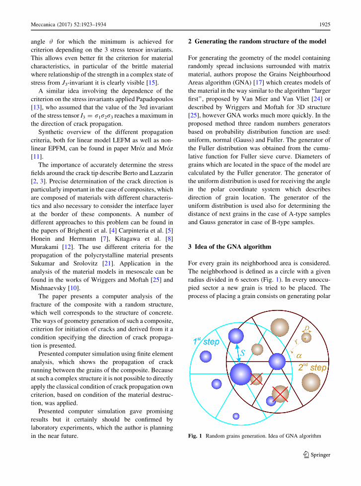
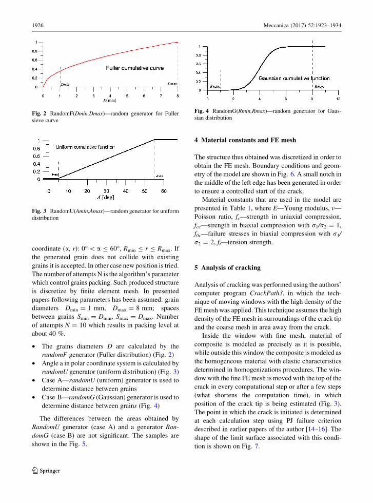
proposed method three random numbers generators

based on probability distribution function are used:

uniform, normal (Gauss) and Fuller. The generator of

the Fuller distribution was obtained from the cumu-

lative function for Fuller sieve curve. Diameters of

grains which are located in the space of the model are

calculated by the Fuller generator. The generator of

the uniform distribution is used for receiving the angle

in the polar coordinate system which describes

direction of grain location. The generator of the

uniform distribution is used also for determining the

distance of next grains in the case of A-type samples

and Gauss generator in case of B-type samples.

3 Idea of the GNA algorithm

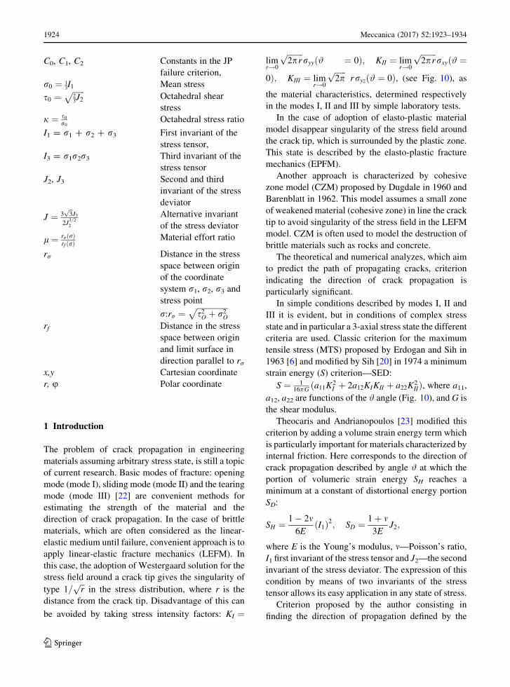
For every grain its neighborhood area is considered.

The neighborhood is defined as a circle with a given

radius divided in 6 sectors (Fig. 1). In every unoccu-

pied sector a new grain is tried to be placed. The

process of placing a grain consists on generating polar

Fig. 1 Random grains generation. Idea of GNA algorithm

Meccanica (2017) 52:1923–1934 1925

123

coordinate (a, r): 0�\ a B 60�, Rmin B r B Rmax. If

the generated grain does not collide with existing

grains it is accepted. In other case new position is tried.

The number of attempts N is the algorithm’s parameter

which control grains packing. Such produced structure

is discretize by finite element mesh. In presented

papers following parameters has been assumed: grain

diameters Dmin = 1 mm, Dmax = 8 mm; spaces

between grains Smin = Dmin, Smax = Dmax. Number

of attempts N = 10 which results in packing level at

about 40 %.

• The grains diameters D are calculated by the

randomF generator (Fuller distribution) (Fig. 2)

• Angle a in polar coordinate system is calculated by

randomU generator (uniform distribution) (Fig. 3)

• Case A—randomU (uniform) generator is used to

determine distance between grains

• Case B—randomG (Gaussian) generator is used to

determine distance between grains (Fig. 4)

The differences between the areas obtained by

RandomU generator (case A) and a generator Ran-

domG (case B) are not significant. The samples are

shown in the Fig. 5.

4 Material constants and FE mesh

The structure thus obtained was discretized in order to

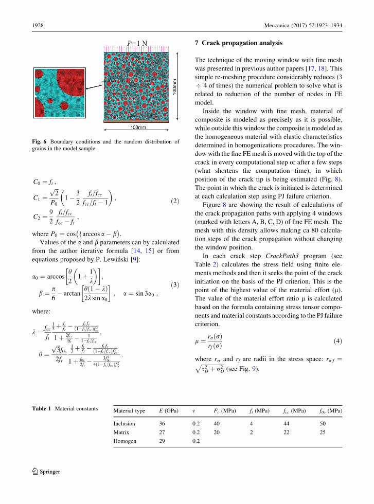
obtain the FE mesh. Boundary conditions and geom-

etry of the model are shown in Fig. 6. A small notch in

the middle of the left edge has been generated in order

to ensure a controlled start of the crack.

Material constants that are used in the model are

presented in Table 1, where E—Young modulus, v—

Poisson ratio, fc—strength in uniaxial compression,

fcc—strength in biaxial compression with r1/r2 = 1,

f0c—failure stresses in biaxial compression with r1/

r2 = 2, ft—tension strength.

5 Analysis of cracking

Analysis of cracking was performed using the authors’

computer program CrackPath3, in which the tech-

nique of moving windows with the high density of the

FE mesh was applied. This technique assumes the high

density of the FE mesh in surroundings of the crack tip

and the coarse mesh in area away from the crack.

Inside the window with fine mesh, material of

composite is modeled as precisely as it is possible,

while outside this window the composite is modeled as

the homogeneous material with elastic characteristics

determined in homogenizations procedures. The win-

dow with the fine FE mesh is moved with the top of the

crack in every computational step or after a few steps

(what shortens the computation time), in which

position of the crack tip is being estimated (Fig. 3).

The point in which the crack is initiated is determined

at each calculation step using PJ failure criterion

described in earlier papers of the author [14–16]. The

shape of the limit surface associated with this condi-

tion is shown on Fig. 7.

Fig. 2 RandomF(Dmin,Dmax)—random generator for Fuller

sieve curve

Fig. 3 RandomU(Amin,Amax)—random generator for uniform

distribution

Fig. 4 RandomG(Rmin,Rmax)—random generator for Gaus-

sian distribution

1926 Meccanica (2017) 52:1923–1934

123

6 PJ failure criterion

The criterion was proposed by author [14, 15] in 1984

in the form:

r0 � C0 þ C1PðJÞs0 þ C2s20 ¼ 0 ð1Þ

where PðJÞ ¼ cos 13arccos aJ � b

� �—function describ

ing the shape of limit surface in deviatoric plane,

r0 ¼ 13I1—mean stress, s0 ¼

ffiffiffiffiffiffi23J2

p—octahedral shear

stress, I1—first invariant of the stress tensor, J2, J3—

second and third invariant of the stress deviator,

J ¼ 3ffiffi3

pJ3

2J3=2

2

—alternative invariant of the stress deviator,

a, b, C0, C1, C2—material constants.

Classical failure criteria, like Huber–Mises, Tresca,

Drucker–Prager, Coulomb-Mohr as well as some new

ones proposed by Lade, Matsuoka, Ottosen, are

particular cases of the general form (1) PJ criterion.

Material constants can be evaluated on the basis of

some simple material test results like:

• fc—failure stress in uniaxial compression,

• ft—failure stress in uniaxial tension,

• fcc—failure stress in biaxial compression at r1/

r2 = 1,

• f0c—failure stress in biaxial compression at r1/

r2 = 2/1,

• fv—failure stress in triaxial tension at r1/r2/

r3 = 1/1/1,

For concrete or rock-like materials some simpli-

fication can be taken on the basis of the Rankine–

Haythornthwaite ‘‘tension cutoff’’ hypothesis: fv =

ft.Values of the material constants C0, C1, C2 can be

calculated from following equations:

Fig. 5 Specimen generated by RandomU procedure—case A, RandomG procedure—case B and the corresponding principal stress

maps

Meccanica (2017) 52:1923–1934 1927

123

C0 ¼ ft ;

C1 ¼ffiffiffi2

p

P0

1 � 3

2

ft=fccfcc=ft � 1

� �;

C2 ¼ 9

2

ft=fccfcc � ft

;

ð2Þ

where P0 ¼ cos 13arccos a� b

� �.

Values of the a and b parameters can by calculated

from the author iterative formula [14, 15] or from

equations proposed by P. Lewinski [9]:

a0 ¼ arccosh2

1 þ 1

k

� �� �;

b ¼ p6� arctan

h 1 � kð Þ2k sin a0

� �; a ¼ sin 3a0 ;

ð3Þ

where:

k ¼ fcc

ft

13þ ft

fc� ft fc

1�ft=fccð Þf 2cc

1 þ 2fcc3ft

� 11�ft=fcc

;

h ¼ffiffiffi3

pf0c

2ft

13þ ft

fc� ft fc

1�ft=fccð Þf 2cc

1 þ f0c2ft� 3f 2

0c

4 1�ft=fccð Þf 2cc

:

7 Crack propagation analysis

The technique of the moving window with fine mesh

was presented in previous author papers [17, 18]. This

simple re-meshing procedure considerably reduces (3

7 4 of times) the numerical problem to solve what is

related to reduction of the number of nodes in FE

model.

Inside the window with fine mesh, material of

composite is modeled as precisely as it is possible,

while outside this window the composite is modeled as

the homogeneous material with elastic characteristics

determined in homogenizations procedures. The win-

dow with the fine FE mesh is moved with the top of the

crack in every computational step or after a few steps

(what shortens the computation time), in which

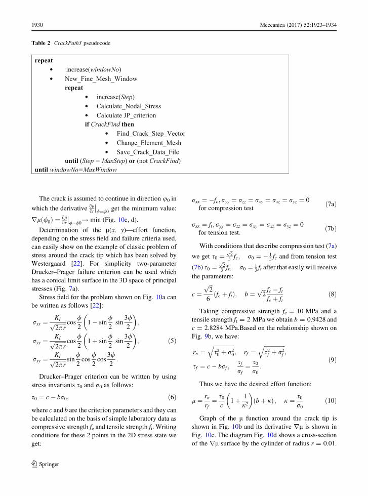
position of the crack tip is being estimated (Fig. 8).

The point in which the crack is initiated is determined

at each calculation step using PJ failure criterion.

Figure 8 are showing the result of calculations of

the crack propagation paths with applying 4 windows

(marked with letters A, B, C, D) of fine FE mesh. The

mesh with this density allows making ca 80 calcula-

tion steps of the crack propagation without changing

the window position.

In each crack step CrackPath3 program (see

Table 2) calculates the stress field using finite ele-

ments methods and then it seeks the point of the crack

initiation on the basis of the PJ criterion. This is the

point of the highest value of the material effort (l).

The value of the material effort ratio l is calculated

based on the formula containing stress tensor compo-

nents and material constants according to the PJ failure

criterion.

l ¼ rrðrÞrf ðrÞ

ð4Þ

where rr and rf are radii in the stress space: rr;f ¼ffiffiffiffiffiffiffiffiffiffiffiffiffiffiffiffis2O þ r2

O

p(see Fig. 9).

Fig. 6 Boundary conditions and the random distribution of

grains in the model sample

Table 1 Material constants Material type E (GPa) v Fc (MPa) ft (MPa) fcc (MPa) f0c (MPa)

Inclusion 36 0.2 40 4 44 50

Matrix 27 0.2 20 2 22 25

Homogen 29 0.2

1928 Meccanica (2017) 52:1923–1934

123

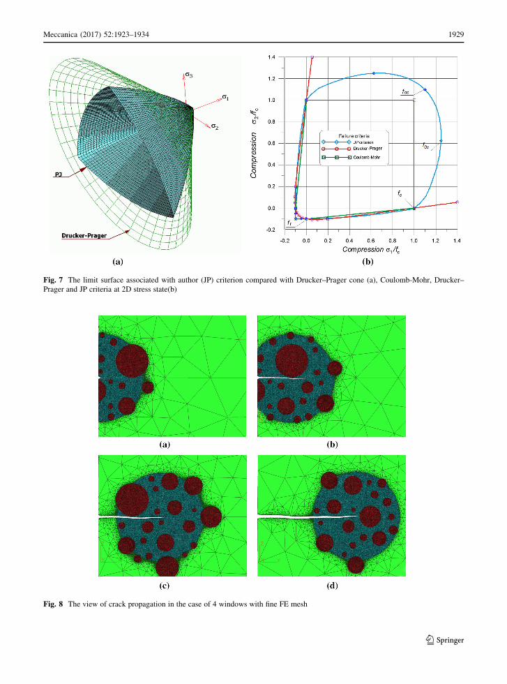
Fig. 7 The limit surface associated with author (JP) criterion compared with Drucker–Prager cone (a), Coulomb-Mohr, Drucker–

Prager and JP criteria at 2D stress state(b)

Fig. 8 The view of crack propagation in the case of 4 windows with fine FE mesh

Meccanica (2017) 52:1923–1934 1929

123

The crack is assumed to continue in direction u0 in

which the derivative olor

/¼/0

get the minimum value:

rlð/0Þ ¼ olor

/¼/0

! min (Fig. 10c, d).

Determination of the l(x, y)—effort function,

depending on the stress field and failure criteria used,

can easily show on the example of classic problem of

stress around the crack tip which has been solved by

Westergaard [22]. For simplicity two-parameter

Drucker–Prager failure criterion can be used which

has a conical limit surface in the 3D space of principal

stresses (Fig. 7a).

Stress field for the problem shown on Fig. 10a can

be written as follows [22]:

rxx ¼KIffiffiffiffiffiffiffiffi2pr

p cos/2

1 � sin/2

sin3/2

� �;

ryy ¼KIffiffiffiffiffiffiffiffi2pr

p cos/2

1 þ sin/2

sin3/2

� �;

rxy ¼KIffiffiffiffiffiffiffiffi2pr

p sin/2

cos/2

cos3/2

:

ð5Þ

Drucker–Prager criterion can be written by using

stress invariants s0 and r0 as follows:

s0 ¼ c� br0; ð6Þ

where c and b are the criterion parameters and they can

be calculated on the basis of simple laboratory data as

compressive strength fc and tensile strength ft. Writing

conditions for these 2 points in the 2D stress state we

get:

rxx ¼ �fc; ryy ¼ rzz ¼ rxy ¼ rxz ¼ ryz ¼ 0

for compression testð7aÞ

rxx ¼ ft; ryy ¼ rzz ¼ rxy ¼ rxz ¼ ryz ¼ 0

for tension test:ð7bÞ

With conditions that describe compression test (7a)

we get s0 ¼ffiffi2

p

3fc; r0 ¼ � 1

3fc and from tension test

(7b) s0 ¼ffiffi2

p

3ft; r0 ¼ 1

3ft after that easily will receive

the parameters:

c ¼ffiffiffi2

p

6fc þ ftð Þ; b ¼

ffiffiffi2

p fc � ft

fc þ ftð8Þ

Taking compressive strength fc = 10 MPa and a

tensile strength ft = 2 MPa we obtain b = 0.9428 and

c = 2.8284 MPa.Based on the relationship shown on

Fig. 9b, we have:

rr ¼ffiffiffiffiffiffiffiffiffiffiffiffiffiffiffis2

0 þ r20

q; rf ¼

ffiffiffiffiffiffiffiffiffiffiffiffiffiffiffis2f þ r2

f

q;

sf ¼ c� brf ;sfrf

¼ s0

r0

:ð9Þ

Thus we have the desired effort function:

l ¼ rr

rf¼ s0

c1 þ 1

j2

� �bþ jð Þ ; j ¼ s0

r0

ð10Þ

Graph of the l function around the crack tip is

shown in Fig. 10b and its derivative rl is shown in

Fig. 10c. The diagram Fig. 10d shows a cross-section

of the rl surface by the cylinder of radius r = 0.01.

Table 2 CrackPath3 pseudocode

repeatincrease(windowNo)New_Fine_Mesh_Windowrepeat

increase(Step)Calculate_Nodal_StressCalculate JP_criterion

if CrackFind thenFind_Crack_Step_VectorChange_Element_MeshSave_Crack_Data_File

until (Step = MaxStep) or (not CrackFind)until windowNo=MaxWindow

1930 Meccanica (2017) 52:1923–1934

123

Fig. 9 Definition of the material effort ratio l, a JP criterion, b Drucker–Prager criterion

Fig. 10 Material effort ratio for classical Westergaard stress

field near crack tip, Drucker -Prager failure criterion was used

for l definition, a) coordinates near crack tip, b) concentration of

the effort ratio near crack tip, c) field of the rl—effort ratio

derivative, d) rl—u dependency at r = 0.01 ? u0 = 0

Meccanica (2017) 52:1923–1934 1931

123

Visible is the minimum point of this section, which,

according to the prediction occurs at u = 0.

Assuming other criteria (e.g. JP) and material

heterogeneity we get much more complex terms

describing the angle of crack propagation. Charts of

the material effort for the heterogeneous composite

with strong circular inclusions is shown in Fig. 11. It

was made on a FEA mesh based on stress calculated

numerically, JP condition was used.

Known and described in the literature are several

criteria of crack propagation, starting from the classic

conditions of Griffith’s maximum energy release rate

criterion by the condition of minimum strain energy

density proposed by Erdogan and Sih and somewhat

similar to condition described above, Papadopoulos

Det-criterion [13]. Overview of the many conditions

of crack propagation in homogeneous materials can be

found in the paper of Mroz and Mroz [11].

Conditions for predicting of cracks propagation in

heterogeneous materials such as composites, geoma-

terials and polycrystalline materials are much more

complex. There may be mentioned, for example, the

approach proposed by Honein and Herrmann [7] and

Sukumar and Srolovitz [21], where considered mate-

rials similar to that described in this work.

The proposed simple, local criterion for composites

with brittle matrix makes it easy to predict the

direction of crack propagation. Criterion has been

repeatedly used by the author and colleagues in

numerical analyzes of crack rocks and concrete, where

the predominant failure modes corresponding to the

open crack—mode I.

After finding the direction of the crack propagation,

a FE mesh is modified in surroundings of the crack tip

in order to add the next crack segment with the length

equal to the size of the cracked element. The procedure

Fig. 11 Values of the material effort ratio l near the crack tip and grain border

-50 -48 -46 -44 -42 -40 -38 -36 -34 -32 -30 -28 -26 -24Y [mm]

-0.5

0

0.5

1

1.5

2

2.5

Z[m

m]

1 11 21 31 41 51 61 711 11 21 31 41 51 61 71

1 11 21 31 41 5161

71 811

11

233343

53

Crack path calculationsWindow AWindow BWindow CWindow DModel 2Model 3

Fig. 12 The path of the crack propagation

1932 Meccanica (2017) 52:1923–1934

123

is carried on until the demanded number of steps is

achieved or the crack stops propagating [18, 19],

Fig. 12.

The propagation of the analyzed crack was per-

formed on FE mesh consisted of 20,498 (window A)

up to 42,326 (window C) nodes. For comparison

purpose calculations for models without the windows

were also performed: Model 2—16,032 and Model

3—31,311 nodes. In the last two cases, paths of the

crack are less stable and the calculations times are

comparable to the time needed for the Model 1. The

hypothetical model 4, with mesh density comparable

to the model 1, would require execution time 20 times

longer to calculate 10 steps of the crack.

Windows with the fine FE mesh presented in this

paper were generated as a circle with the radius r %10 mm, created around of the crack tip. Grains lying

on the border of the circle were included in this

domain in order to make impossible creation of

artificial effects of the stress concentration on the

border of homogenized material. Model shown on

Fig. 3 (Model 1 with windows A, B, C, D) was created

assuming material constants given in the Table 1.

Other methods of analysis of crack propagation in

the heterogeneous materials were described e.g. in

papers: Bazant [1], Carpinteri and others. [5], Mish-

naevsky [10].

Known and described in the literature are several

criteria of crack propagation, starting from the classic

conditions of Griffith’s maximum energy release rate

criterion by the condition of minimum strain energy

density proposed by Erdogan and Sih and somewhat

similar to condition described above, Papadopoulos

Det-criterion [13]. Overview of the many conditions

of crack propagation in homogeneous materials can be

found in the paper of Mroz and Mroz [11].

Conditions for predicting of cracks propagation in

heterogeneous materials such as composites, geoma-

terials and polycrystalline materials are much more

complex. There may be mentioned, for example, the

approach proposed by Honein and Herrmann [7] and

Sukumar and Srolovitz [21], where considered mate-

rials similar to that described in this work.

8 Conclusions

Simulation of the crack propagation for composite

materials by FE method requires precise remeshing

technique and very fine element mesh. The method of

movable window with high mesh density seems to be a

promising solution technique for problems requiring a

high discretization level at a local scale. Cracking

analyses of geomaterials with random structures fit

naturally in this group. The CrackPath3 computer

code uses the new criterion for prediction of the crack

propagation direction which is simpler than suggested

for polycrystalline materials by Sukumar and Srolo-

vitz [21].

The proposed simple, local criterion for composites

with brittle matrix makes it easy to predict the

direction of crack propagation. Criterion has been

repeatedly used by the author in numerical analyzes of

crack in rock and concrete, where the predominant

failure modes corresponding to the open crack—mode

I. Presented computer simulation gave promising

results but it certainly should be confirmed by

laboratory experiments. Certainly would be interest-

ing testing the behavior of crack propagation in three-

dimensional models. This type analysis with FE

models is planned as the subject of next works of the

author.

Open Access This article is distributed under the terms of the

Creative Commons Attribution 4.0 International License (http://

creativecommons.org/licenses/by/4.0/), which permits unrest-

ricted use, distribution, and reproduction in any medium, pro-

vided you give appropriate credit to the original author(s) and

the source, provide a link to the Creative Commons license, and

indicate if changes were made.

References

1. Bazant Z (2002) Concrete fracture models: testing and

practice. Eng Fract Mech 69:165–205

2. Berto F, Lazzarin P (2010) On higher order terms in the

crack tip stress field. Int J Fract 161:221–226

3. Berto F, Lazzarin P (2013) Multiparametric full-field rep-

resentations of the in-plane stress fields ahead of cracked

components under mixed mode loading. J Fatigue 46:16–26

4. Brighenti R, Carpinteri A, Spagnoli A (2014) Influence of

material micro-voids and heterogeneities on fatigue crack

propagation. Acta Mech 225:3123–3135

5. Carpinteri A, Chiaia B, Cornetti P (2003) On the mechanics

of quasi-brittle materials with a fractal microstructure. Eng

Fract Mech 70:2321–2349

6. Erdogan F, Sih GC (1963) On the crack extension in plates

under plane loading and transverse shear. J Basic Engng.

85:519–527

7. Honein T, Herrmann G (1990) On bonded inclusions with

circular or straight boundaries in plane elastostatics. J Appl

Mech Trans ASME 57:850–856

Meccanica (2017) 52:1923–1934 1933

123

8. Kitagawa H, Yuuki R, Ohira T (1975) Crack-morphological

aspects in fracture mechanics. Eng Fract Mech 7:515–529

9. Lewinski P (1996) Nieliniowa analiza osiowo-syme-

trycznych konstrukcji powłokowych. Prace Naukowe PW

131:73

10. Mishnaevsky L (2007) Computational mesomechanics of

composites. Wiley, New York

11. Mroz KP, Mroz Z (2010) On crack path evolution rules. Eng

Fract Mech 77:1781–1807

12. Murakami Y (2002) Metal fatigue: effects of small defects

and nonmetallilc inclusions. Elsevier, Amsterdam

13. Papadopoulos GA (1987) The stationary value oh the third

stress invariant as a local fracture parameters (Det-crite-

rion). Eng Fract Mech 27:643–652

14. Podgorski J (1984) Limit state condition and the dissipation

function for isotropic materials. Arch Mech 36:323–342

15. Podgorski J (1985) General failure Criterion for isotropic

media. J Eng Mech ASCE 111:188–201

16. Podgorski J (2002) Influence exerted by strength criterion

on direction of crack propagation in the elastic-brittle

material. J Min Sci 38(4):374–380

17. Podgorski J, Nowicki T, Jonak J (2006) Fracture analysis of

the composites with random structure, IWCMM 16, Sep

25–25, 2006. Lublin, Poland

18. Podgorski J, Nowicki T (2007) Fine mesh window tech-

nique used in fracture analysis of the composites with ran-

dom structure, CMM-2007 - Computer Methods in

Mechanics, June 19–22, 2007. Łodz-Spała, Poland

19. Podgorski J, Sadowski T, Nowicki T (2008) Crack propa-

gation analysis in the media with random structure by fine

mesh window technique, WCCM8, ECCOMAS 2008, June

30–July 5, 2008. Venice, Italy

20. Sih GC (1973) Some basic problems in fracture mechanics

and new concepts. Eng Fract Mech vpl. 5:365–377

21. Sukumar N, Srolovitz DJ (2004) Finite element-based

model for crack propagation in polycrystalline materials.

Comput Appl Math 23(2–3):363–380

22. Sun CT, Jin ZH (2012) Fracture Mechanics. Academic,

Elsevier Inc, Amsterdam

23. Theocaris PS, Andrianopoulos NP (1982) The Mises elas-

tic–plastic boundary as the core region in fracture criteria.

Eng Fract Mech 16:425–432

24. Van Mier JGM, Van Vliet MRA (2003) Influence of

microstructure of concrete on size/scale effects in tensile

fracture. Eng Fract Mech 70:2281–2306

25. Wriggers P, Moftah SO (2006) Mesoscale models for con-

crete: homogenisation and damage behaviour. Finite Elem

Anal Des 42:623–636

1934 Meccanica (2017) 52:1923–1934

123