2.0 simple mechanism - prog.lmu.edu.ng 312 lectu… · application of kutzbach criterion to plane...
TRANSCRIPT

2.0 Simple Mechanism
As earlier mentioned a machine is a device which receives energy and transforms it into
some useful work. A machine consists of a number of parts or bodies. We shall study here the
Mechanisms of various parts or bodies from which the machine is assembled.
Kinematic Link or Element
Each part of a machine, which moves relative to some other parts, is known as a
Kinematic link (or simply link) or element. A link may consist of several parts, which are rigidly
fastened together, so that they do not move relative to one another. A link should have the
following characteristics.
1. It should have relative motion and
2. It must be a resistant body. (A body is said to be a resistance if it is capable of
transmitting the required forces with negligible deformation).
Types of Links
1. Rigid link: A rigid link is one which does not undergo any deformation while
transmitting motion. Strictly speaking, rigid links don not exists. However as the
deformation of a connecting rod, crank etc. of a reciprocating steam engine is not
appreciable, they can be considered as rigid links.
2. Flexible Link: A flexible link is one which is partly deformed in a manner not to affect
the transmission of motion. For example, belts, ropes, chains and wires are flexible links
and transmit tensile forces only.
3. Fluid Link: The link which is formed by having a fluid in a receptacle and the motion is
transmitted through the fluid by pressure or compression only, as in the case of hydraulic
presses, jacks and brakes.
Kinematic Pair
Two links which are connected together is such as way that their relative motion is
completely or successfully constrained forms a kinematic pair.
Types of Constrained Motions
The following are the three types of constrained motions:
1. Completely constrained motion: When the motion between a pair is limited to a definite
direction irrespective of the direction of force applied then the motion is said to be a completely
constrained motion.

Fig.2.1 Square bar in a square hole Fig.2.2. Shaft with collar in a circular hole
For example, the piston and cylinder (in a steam engine) form a pair and the motion of the piston
is limited to a definite direction (i.e. it will only reciprocate) relative to the cylinder irrespective
of the direction of motion of the crank.
The motion of a square bar in a square hole as in fig. 2.1 and motion of a shaft with
collars at each end in a circular hole, as in fig. 2.2 are examples of completely constrained
motion.
2. Incompletely constrained motion: when the motion between a pair can take place in
more than one direction, then the motion is called an incompletely constrained motion.
The change in the direction of impressed force may alter the direction of relative motion
between the pair. A circular bar or shaft in a circular hole as shown in fig. 2.3, is an
example of an incompletely constrained motion as it may either rotate or slide in a hole.
3. Successfully constrained motion: When the motion between the elements, forming a
pair, is such that the constrained motion is not completed by itself, but by some other
meant, then the motion is said to be successfully constrained motion. Consider a shaft in
a foot-step bearing in fig. 2.4, the shaft may rotate in a bearing or may move upwards (in
completely constrained motion), but if the load is placed on the shaft to prevent axial
upward movement of the shaft, then the motion of the pair is said to be successfully
constrained motion.

Kinematic Chain
When the Kinematic pairs are coupled in such a way that the last link is joined to the first
link to transmit definite motion (i.e completely or successfully constrained motion), it is called a
Kinematic chain. This is to say that a Kinematic chain may be defined as a combination of
kinematic pairs, joined in such a way that each link forms a part of two parts and the relative
motion between the links or elements is completely or successful constrained. For example, the
crankshaft of an engine forms a Kinematic pair with the bearings which a fixed in a pair, the
connecting rod with the crank forms a second kinematic pair, the piston with connecting rod
forms a third and the piston with the cylinder forms a fourth pair. The combination of these links
is a Kinematic chain.
Types of Kinematic chains
The most important kinematic chains are those which consist of four lower pairs, each
pair being a sliding pair or a turning pair. The following are the three types of Kinematic chains
with four lower pairs.
1. Four bar chain or quadric cycle chain
2. Single slider crank chain, and
3. Double slider crank chain.
Mechanism
When one of the links of a kinematic chain is fixed, the chain is known as Mechanism,
while the mechanism with more than four links is known as compound mechanism. When a
mechanism is required to transmit power or to do some particular type of work, it becomes a
machine.
Number of Degree of Freedom for Plane Mechanism
In the Design or analysis of a mechanism, one of the most important concern is the
number of degree of freedom (also called movability) of the mechanism. It is defined as the
number of input parameters (usually pair variables) which must be independently controlled is
order to bring the mechanism into a useful engineering purpose.
Application of Kutzbach Criterion to Plane Mechanisms
Kutzbach criterion for determining the number of degrees of freedom or movability (n) of
a plane mechanism is
n = 3 (l – 1) – 2j – h.

Note:
a. When n = 0, then the mechanism forms a structure and not relative motion between the
links is possible.
b. When n = 1, then the mechanism can be driven by a single input motion.
c. When n = 2, then two separate input motions are necessary to produce constrained
motion for the mechanism.
d. When n = -1 or less, then there are redundant constraints in the chain and it forms a
statically indeterminate structure.
Velocity in Mechanisms
There are two important methods of determining the velocity of any point on a link in a
mechanism out of many.
1. Instantaneous centre method
2. Relative velocity method.
- Velocity of a point on a link by Instantaneous centre method: The instantaneous
centre method of analyzing the motion in a mechanism is based upon the concept that any
displacement of a body (or rigid link) having motion in one plane, can be considered as a
pure rotational motion of a rigid link as a whole about some centre, known as
instantaneous centre or virtual centre of rotation.
- Number of Instantaneous centre in a mechanism
The number of instantaneous centres in a constrained kinematic chain is equal to the
number of possible combinations of two links.
The number of pairs of links or the number of instantaneous centres is the number of
combinations of n links taken two at a time.
Mathematically, number of instantaneous centres

N=
linksofNumbernwherenn
,2
1
- Types of Instantaneous centres
The instantaneous centres for a mechanism are of the following types
1. Fixed instantaneous centres,
2. Permanent instantaneous centres
3. Neither fixed nor permanent instantaneous centres.
The first two types i.e. fixed and permanent instantaneous centres, are together known as
primary instantaneous centres and the third type is known as secondary instantaneous centres.
Fig. 2.5: Types of instantaneous centre
Consider a four bar mechanism ABCD as shown is fig. 2.5. the instantaneous centres (N)
in a four bar mechanism is given by
N =
62
144
2
1
nn
The instantaneous centres I12 and I14 are called the fixed instantaneous centres as they
remain in the same place for all configuration of the mechanism. The instantaneous centres I23
and I34 are the permanent instantaneous centres as they move when the mechanism moves, but
the joints are of permanent nature. The instantaneous centres I13 and I24 are neither fixed nor
permanent instantaneous centres as they vary with the configuration of the mechanism.
Method of locating Instantaneous Centres in a Mechanism
Consider a pin jointed four bar mechanism as shown which in fig. 2.6 (a). The following
procedure is adopted for locating instantaneous centres.
1. First, Determine the number of instantaneous (N) by using the relation.

N =
62
144
2
1
nn
The instantaneous centres I12 and I14 are called the fixed instantaneous centres as they
remain in the same place for all configuration of the mechanism. The instantaneous centres I23
and I34 are the permanent Instantaneous centres as they move when the mechanism moves, but
the joints are of permanent nature. The instantaneous centres I13 and I14 are neither fixed nor
permanent instantaneous centres as they vary with the configuration of the mechanism.
Method of Locating Instantaneous Centres in a Mechanism
Consider a pin jointed four bar mechanism as shown in fig.2.6 (a). The following
procedure is adopted for locating instantaneous centres.
1. First, Determine the number of instantaneous centre (N) by using the relation N =
2
1nn, linksofNumbernwhere
In this case, N = 6
2. Make a list of all the Instantaneous centres in a mechanisms, since for a four bar
mechanism, there are six instantaneous centres, therefore these centres are listed as
shown in the table below (known as book – keeping table).
3. Locate the fixed and permanent instantaneous centres by inspection I12 and I14 are fixed
instantaneous centres and I23 and I34 are permanent instantaneous centres.
Links 1 2 3 4
Instantaneous centres (6 in
number)
12
13
14
23
24
34 -
(a) Four bar Mechanism (b) Circle diagram

4. Locate the remaining neither fixed nor permanent instantaneous centres (or secondary
centres) by Kennedy’s theorem. This is done by circle Diagram as shown in fig. 2.6(b),
mark points on a circle equal to the number of links in a mechanism. In this case, mark 1,
2, 3 and 4 on the circle.
5. Join the points by solid lines to show that these centres are already found. In the circle
Diagram these lines are 12, 23, 34 and 14 to indicate the centres I12, I23, I34 and I14.
6. In order to find the other two instantaneous, join two such points that the line joining
them form two adjacent triangles in the circle diagram. i.e. In the case of fig.2.6(b), join 1
and 3 to form the triangle 123 and 341 and the Instantaneous centre I13 which lie on the
intersection of I12 I23 and I14 and I34, produced if necessary on the mechanisms. Thus the
instantaneous centre I13 is located. Join 1 and 3 by a dotted line on the circle diagram and
mark number 5 on it. Similarly the instantaneous centre I24 will lie on the intersection of
I12 I14 and I23 I24, produced if necessary, on the mechanism. This I24 is located. Join 2 and
4 by a dotted line on the circle diagram and mark 6 on it.
Example 1
In a pin jointed four bar mechanism, as shown in the fig. below AB 300mm, Bc = CD =
360mm, and AD =600mm. The angle BAD = 60. The crank AB rotates uniformly at 100
r.p.m. Locate all the instantaneous centres and find the angular velocity of the link BC.
Solution
NAB = 100 r.p.m.
ωAB = sradx
/47.1060
1002
Since crank length AB= 300mm = 0.3m, therefore velocity of point B on link AB.
sm
ABV ABB
/14.3
3.047.10

Location of Instantaneous centre
Follow the method of locating instantaneous centre as previously discussed..
i.e N = 6. ………………………….. (n = 4)
Angular velocity of the link BC
ωBC = 5.0
141.3
13
BI
VB
= 6. 282 rad/s.
Example 2
Locate all the instantaneous centres of the slider crank mechanism as shown below. The
lengths of crank OB and connecting rod AB are 100mm and 400mm respectively, if the
crank rotates clockwise with an angular velocity of 10 rad/s, find.
(a) Velocity of the slider A and
(b) Angular velocity of the connecting rod AB.
Solution
Given: ωoB = 10rad/s, OB = 100mm = 0.1m
Linear velocity of the crank OB
VoB = VB = ωoB x OB
= 10 x 0.1 = 1m/s.
Location of instantaneous centres.

Since there are four links (n = 4), therefore the number of instantaneous centres
N=
62
144
2
1
nn
2. For a four link mechanism, the book keeping table may be drawn as previously discussed.
3. Locate the fixed and permanent instantaneous centre by inspection. These centres are I12, I23
and I34 as shown below, since the slider (link 4) moves on a straight surface (link 1), therefore
the instantaneous centre I14 will lie at infinity.
4. Locate the other two remaining neither fixed nor permanent instantaneous centres, by
Kennedy’s theorem. This is done by circle diagram.
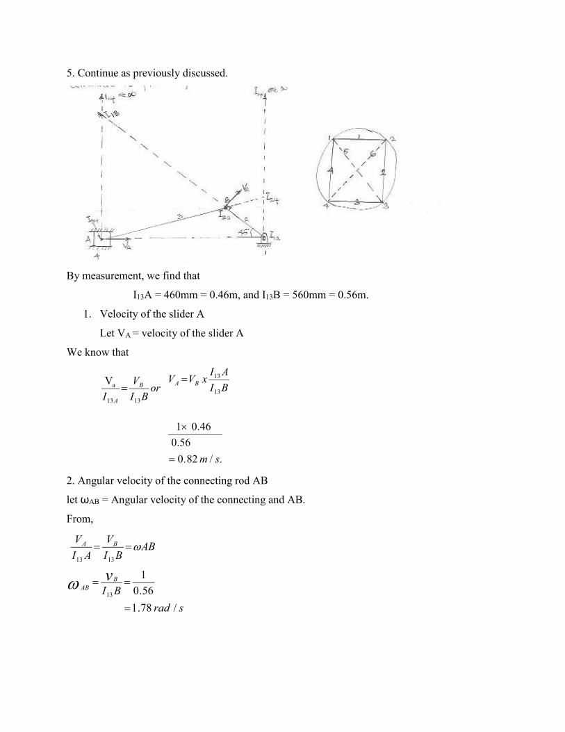
5. Continue as previously discussed.
By measurement, we find that
I13A = 460mm = 0.46m, and I13B = 560mm = 0.56m.
1. Velocity of the slider A
Let VA = velocity of the slider A
We know that
orBI
V
IB
A 1313
aV BI
AIxVV BA
13
13
./82.0
56.0
46.01
sm
2. Angular velocity of the connecting rod AB
let ωAB = Angular velocity of the connecting and AB.
From,
srad
BI
ABBI
V
AI
V
vB
AB
BA
/78.1
56.0
1
13
1313

Example 3
A mechanism as shown below has the following dimensions: OA = 200mm, AB = 1.5,
BC =600mm; CD = 500mm and BE = 400mm.
Locate the instantaneous centres. If the crank OA rotates Uniformly at 120 r.p.m clockwise, find
a. The velocity of B, C and D
b. The angular velocity of the link, AB, BC, and CD.
Solution
NoA = 120 r.p.m or ω0A = ./57.1260
1202srad
Since the length of crank OA = 200mm = 0.2m, therefore linear velocity of crank OA
VoA =VA =ωoA x OA = 12.57x 0.2
2.514 m/s.
Location of instantaneous centres
1. Since n = 6, N = 15
2. Make a list of the instantaneous centres in a mechanism. Since the mechanism has 15
instantaneous centres, therefore these centres are listed in the book keeping table.
Links 1 2 3 4 5 6
Instantaneous
Centre
15 in numbers
12
13
14
15
16
23
24
25
26
34
35
36
45
46
56
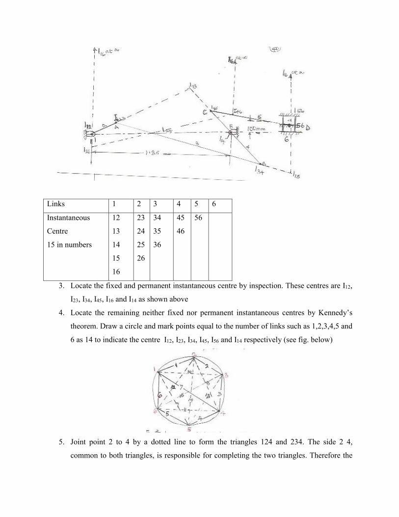
3. Locate the fixed and permanent instantaneous centre by inspection. These centres are I12,
I23, I34, I45, I16 and I14 as shown above
4. Locate the remaining neither fixed nor permanent instantaneous centres by Kennedy’s
theorem. Draw a circle and mark points equal to the number of links such as 1,2,3,4,5 and
6 as 14 to indicate the centre I12, I23, I34, I45, I56 and I14 respectively (see fig. below)
5. Joint point 2 to 4 by a dotted line to form the triangles 124 and 234. The side 2 4,
common to both triangles, is responsible for completing the two triangles. Therefore the
instantaneous centre I24 lies on the intersection of I12 I14 and I23 I34 produced if necessary.
Thus centre I24 is located. Mark number 8 on the dotted line 24 (because seven centres
have already been located)
6. Now join point 1 to 5 by a dotted line to form the triangle 1 4 5 and 1 5 6. The side 1 5,
common to both triangle, is responsible for completing the two triangles. Therefore the
instantaneous centres I15 lies on the intersection of I15 is located. Mark number 9 on the
dotted line 15.
7. Join point 1 to 3, …… for No 10
8. Join point 4 to 6 …… for No 11
9. Join point 2 to 6 ……for No 12
10. Similarly, the 13th, 14th and 15th instantaneous centres (i.e. I35, I25 and I36) may be
located by joining the point 3 to 5, 2 to 5 and 3 to 6 respectively.
By measurement, we find that
I13 A = 840mm = 0.84m, I13B = 107mm = 1.07m; I14B = 400mm = 0.4m
I14C = 200mm = 0.2m; I15 C = 740mm = 0.74m; I15D = 500mm = 0.5.
a) Velocity of Points B, C, and D
Let VB, VC and VD = velocity of the point B, C and D respectively
mls
BIxAI
VV
BI
V
AI
V
AB
BA
2.3
84.0
514.213
13
1313
Again
mls
xCIxBI
VV
CI
V
BI
V
BC
cB
6.1
2.04.0
2.314
14
1414
Similarly,
mls
DIxCI
VV
DI
V
CI
V
DC
DC
08.1
5.074.0
6.15
15
1315
2. Angular velocity of the link AB, BC and CD
Let CDACAB and , = Angular velocity of the links AB, BC, and CD reporting
sradCI
V
sradBI
V
sradAI
V
CCD
BBC
AAB
/16.274.0
6.1
/84.0
2.3
/99.284.0
514.2
15
14
13
Velocity in mechanism (relative velocity method)
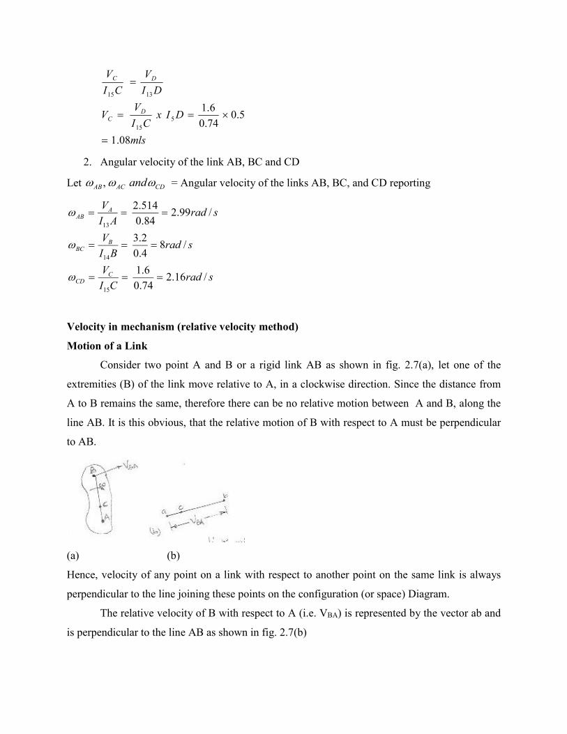
Motion of a Link
Consider two point A and B or a rigid link AB as shown in fig. 2.7(a), let one of the
extremities (B) of the link move relative to A, in a clockwise direction. Since the distance from
A to B remains the same, therefore there can be no relative motion between A and B, along the
line AB. It is this obvious, that the relative motion of B with respect to A must be perpendicular
to AB.
(a) (b)
Hence, velocity of any point on a link with respect to another point on the same link is always
perpendicular to the line joining these points on the configuration (or space) Diagram.
The relative velocity of B with respect to A (i.e. VBA) is represented by the vector ab and
is perpendicular to the line AB as shown in fig. 2.7(b)

Let ω = Angular velocity of the link AB about A.
We know that the velocity of any point B with respect to A.
VBA = )(............................ iABab
Similarly, the velocity of any point C on AB with respect to A
VCA = )(........................... iiACac
From equation (i) and (ii).
AB
AC
AB
AC
ab
ac
V
V
BA
CA .
.
Velocity of a point on a link by relative velocity method
Consider two points A and B on a link as shown in fig 2.8(a). Let the absolute velocity of
the point A ie. VA is known in magnitude and direction and the absolute velocity of the point B
ie. VB is known in direction only. Then the velocity of B may be determined by drawing the
velocity diagram as shown in fig. 2.8(b).
(a) Motion of points on a link (b) Velocity Diagram
The velocity diagram is drawn as follows:
1. Take some convenient point O, known as pole
2. Through O, draw Oa parallel and equal to VA, to some suitable scale
3. Through a, draw a line perpendicular to AB of fig. 2.8(a). this line will represent the
velocity B with respect to A, i.e, VBA.
4. Through O, draw a line parallel to VB intersecting the line of VBA at b.
5. Measure ob, which gives the required velocity of point B (VB), to the scale.
Note:

1. The vector ab which represents the velocity of B with respect to A (VBA) is known as
velocity of image of the link AB.
2. The absolute velocity of any point C on AB may be determined by dividing vector ab at c
in the same ratio as C divides AB. In other words
AB
AC
ab
ac
3. The absolute velocity of any other point D outside AB as shown in fig. 2.8(a), may also
be obtained by completing the velocity triangle abd and similar to triangle ABD, as
shown in fig. 2.8(b).
4. The angular velocity of the link AB may be found by dividing relative velocity of B with
respect to A (i.e. BA) by the length of link AB. Mathematically, angular velocity of the
link AB.
ωAB = AB
ab
AB
VBA
Velocities in slider crank mechanism
A slider crank mechanism is shown in fig. 2.9(a). The slider is attached to the connecting
rod AB. Let the radius of crank OB be r and let it rotates in a clockwise direction, about the point
O with uniform angular velocity W rad/s. therefore the velocity of B i.e VB is known in
magnitude and direction. The slider reciprocates along the line of stroke A0.
(a) Slider Crank Mechanism (b) Velocity Diagram
Rubbing velocity at a pin joint

The links in a mechanism are mostly connected by means of pin joints. The rubbing
velocity is defined as the algebraic sum between the angular velocities of the two links which are
connected by pin joints, multiplied by the radius of the pin.
Consider two links OA and 0B connected by means of pin joints O as shown in fig. 2.10
According to the definition,
Rubbing velocity at the pin joint o
= (�� � ��)r, if the links move in the same direction
= (�� � ��)r, if the links move in the opposite direction.
Note:
When the pin connects one sliding member and other turning member; the angular
velocity of the sliding member is zero. In such cases
Rubbing velocity at the pin joint = �.r
Example 1
In a four bar chain ABCD, AD is fixed and is 150mm long. The crank AB is 40mm long
and rotates at 120 r.p.m clockwise, while the link CD = 80mm Oscillates about D. Bc and AD
are of equal length. Find the angular velocity of CD when angle BAD=600.
Solution
NBA = 120 r.p.m, ωBA = sradX
/568.1260
1202
The length of crank AB = 40mm = 0.04m, therefore velocity B with respect to A or velocity of B
(since A is a fixed point).
VBA= VB = ωBA x AB = 12.568 x 0.04
= 0.503mls

First of all, draw the space diagram to some suitable scale, as shown in fig. 2.11(a) above and the
velocity diagram, as shown in fig 2.11(b) as discussed below.
1. Since the link AD is fixed, therefore point a and d are taken as one point in the velocity
diagram. Draw vector ab perpendicular to BA, to some suitable scale, to represent the
velocity B with respect to A or simply velocity of B (ie. VBA or VB) such that
Vector ab = VBA = VB = 0.503 mls
2. Now from point b, draw vector bc perpendicular to CB to represent the velocity of C
with respect to B (ie. VCB) and from point d, draw vector dc perpendicular to CD to
represent the velocity of C with respect to D or simply velocity of C (i.e. VCD or VC). The
vector bc and dc intersect at C.
By measurement, we find that
VCD = VC = vector dc = 0.385mls
We know that, CD = 80mm = 0.08m
-: Angular velocity of link CD,
WCD = 08.0
385.0
DC
VCD
= 4.8 rad/s. (clockwise about D)
Example 2: The crank and connecting rod of a theoretical steam engine are 0.5m and 2m long
respectively, the crank makes 180r.p.m in the clockwise direction. When it has turned 450 from
the inner dead centre position, determine:
a. Velocity of piston
b. Angular velocity of connecting rod.
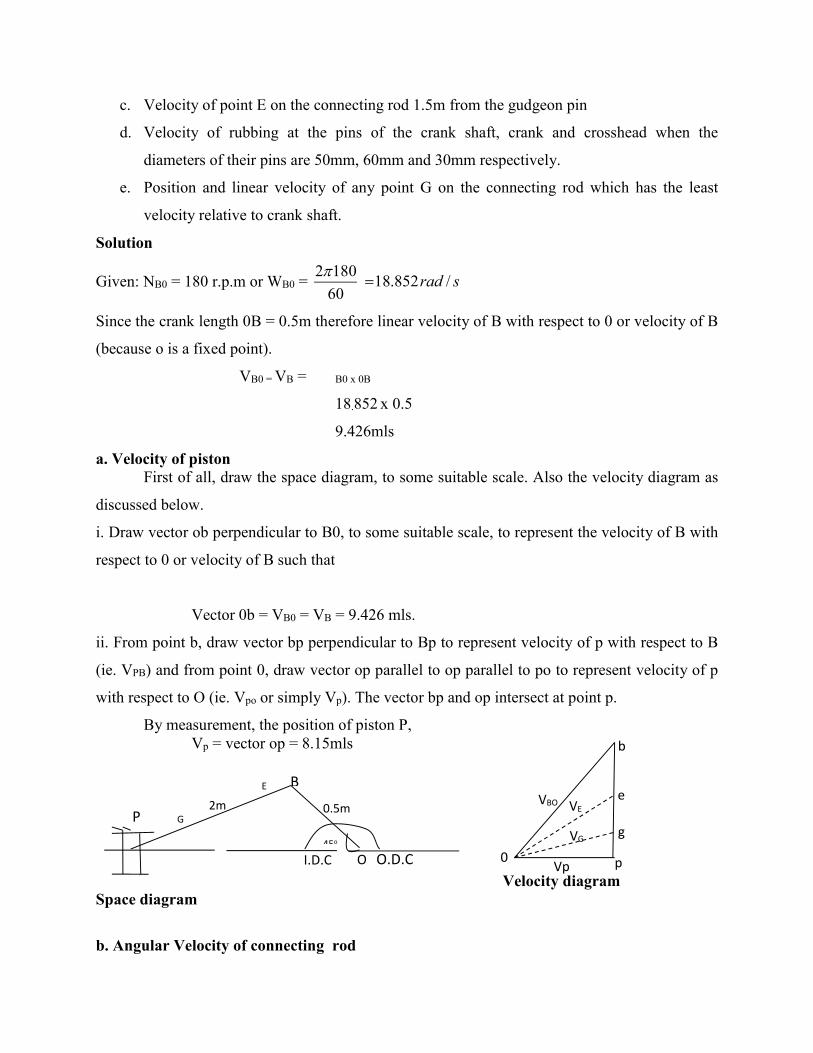
c. Velocity of point E on the connecting rod 1.5m from the gudgeon pin
d. Velocity of rubbing at the pins of the crank shaft, crank and crosshead when the
diameters of their pins are 50mm, 60mm and 30mm respectively.
e. Position and linear velocity of any point G on the connecting rod which has the least
velocity relative to crank shaft.
Solution
Given: NB0 = 180 r.p.m or WB0 = srad /852.1860
1802
Since the crank length 0B = 0.5m therefore linear velocity of B with respect to 0 or velocity of B
(because o is a fixed point).
VB0 = VB = B0 x 0B
18.852 x 0.5
9.426mls
a. Velocity of piston First of all, draw the space diagram, to some suitable scale. Also the velocity diagram as
discussed below.
i. Draw vector ob perpendicular to B0, to some suitable scale, to represent the velocity of B with
respect to 0 or velocity of B such that
Vector 0b = VB0 = VB = 9.426 mls.
ii. From point b, draw vector bp perpendicular to Bp to represent velocity of p with respect to B
(ie. VPB) and from point 0, draw vector op parallel to op parallel to po to represent velocity of p
with respect to O (ie. Vpo or simply Vp). The vector bp and op intersect at point p.
By measurement, the position of piston P, Vp = vector op = 8.15mls
Velocity diagram Space diagram
b. Angular Velocity of connecting rod
g
Vp p
e
b
VBO
0
VG
VE
O O.D.C I.D.C
P G 2m
E B
0.5m
45o

From the velocity diagram, the velocity of P with respect to B,
VPB = Vector bp = 6.8mls
Since the length of connecting rod PB is 2m, therefore angular velocity of the connecting
rod
ωPB = sradPB
VB /4.32
8.6
c. Velocity of point E on the connecting rod
By measurement, velocity of point E.
VE = vector oe = 8.5 mls
Or
Bp
bpxBEbeor
bp
be
Bp
BE
d. Velocity of rubbing
Diameter of crank shaft pin 0,
do = 50mm = 0.05m
Diameter of crank – pin at B,
dp = 60mm = 0.06m
And diameter of cross – head pin,
dc = 30mm = 0.03m
Velocity of rubbing at the pin of crank shaft
= 85.182
05.0
2xd
BOo
= 0.47mls
Velocity of rubbing at the pin of crank
smdPBB
B /47.0)4.385.18(2
06.0
20
……………… (ωBO is clockwise and ωPB is anticlockwise)
Velocity of rubbing at the cross-head
= mlsxxdPB
cc 051.04.3
2
03.0
2

e. The position of point G on the connecting rod which has the least velocity relative to crank
shaft is determined by drawing perpendicular from o to vector bp. Since the length of og will be
the least, therefore the point g represents the required position of G on the connecting rod.
By measurement,
Vector bg = 5 m/s
The position of point G on the connecting rod is obtained as follows
m
x
Bpxbp
bgBG
Bp
BG
bp
bg
47.1
28.6
5
Assignment
1. The Crank OA of the engine Mechanism as shown below rotates at 3600rev/min
anticlockwise. OA =100mm, and the connecting rod AB is 200mm long. Find (a) the
piston velocity (b) the angular velocity of AB (c) the velocity of point C on the rod 50mm
from A.
2. The figure below shows a four-bar mechanism OABQ with a link CD attached to C the
mid-point of AB. The end D of link CD is constrained to move vertically. OA=1m,
AB=1.6m, QB=1.2m, OQ=2.4m and CD=2m. For he position shown, the angular
velocity of Crank OA is 60 rev/min clockwise; find (a) the velocity of D (b) the angular
velocity of CD; (c) the

Acceleration in Mechanism
Acceleration Diagram for a link
Consider two points A and B on a rigid link in the fig 2.13 below. Let the point B moves
with respect to A, with an angular velocity of rad/s and let rad/s2 be the angular
acceleration of the link AB.
Fig. 2.13 (a) Link (b) Acceleration diagram
1. The centripetal or radial component of the acceleration of B with respect to A
BAVABxABlinkoflengthxBAa BA /2221
This radial component of acceleration acts perpendicular to the velocity VBA, In other
words, it acts parallel to the link AB
2. The tangential component of the acceleration of B with respect to A,
AB
ABLinktheofLengthBAa
1

This tangential component of acceleration acts parallel to the velocity VBA. In other
words it acts perpendicular to the link AB.
Acceleration of a point on a Link
Consider two points A and B on the rigid link, as shown in Fig. 2.14(a)
Let the acceleration of the point A i.e. aA is known in magnitude and direction and the direction
of path of B is given. The acceleration of the point B is determined in magnitude and direction
by drawing the acceleration diagram as discussed below.
1. From any point o1, draw vector o1a1 parallel to the direction of absolute acceleration at
point A i.e., aA to some suitable scale, as shown in fig. 2.14(b)
2. We know that the acceleration of B with respect to A i.e. aBA has the following two
components;
(i) Radial component of the acceleration of B with respect to A i.e. arBA and
(ii) Tangential component of the acceleration B with respect to A i.e. atBA. These two
component are mutually perpendicular.
3. Draw vector a1x parallel to the link AB (because radial component of the acceleration of
B with respect to A will pass through AB), such that
Vector AB
VBAaxa
BA2
11
Where, VBA = Velocity of B with respect to A
(a) Points on a link
(b) Acceleration Diagram

Note: The value of VBA may be obtained by drawing the velocity diagram as previously
discussed.
4. From point x, draw vector xb1 perpendicular to AB or vector a1x because tangential
component of B with respect to A i.e. atBA, is perpendicular to radial component arBA)
and through o1 draw a line parallel to the path of B to represent the absolute acceleration
of B i.e. aB. The vector xb1 and o1b1 intersect at b1. Now the values of aB may be
measured, to the scale
5. By joining the points a1 and b1 we may determine the total acceleration of B with respect
to A i.e. aBA. The vector a1b1 is known as acceleration image of the link AB.
6. For any other point C on the link draw triangle a1b1c1 similar to triangle ABC. Now
vector b1c1 represent the acceleration of C with respect to A i.e. aCA. As mentioned
earlier, aCB and aCA will each have two components as follows:
(i) aCB has two components: arCB and at
CB as shown by triangle b1zc1, in which b1z is
parallel to BC and ZC1 is perpendicular to b1Z or BC.
(ii) aCA has two components: arCA and at
CA as shown by triangle a1yc1 in which a1y is
parallel to AC and yc1 is perpendicular to a1y or AC.
7. The angular acceleration of the link AB is obtained by dividing the tangential component
of the acceleration of B with respect to BAtaA To the length of the link. Mathematically,
angular acceleration of the link AB,
AB
a BAt
AB
Acceleration in the slider Crank mechanism
A slider crank mechanism is shown in fig. 2.13 (a). Let the crank OB makes an angle θ
with the inner dead centre (I.D.C) and rotates in a clockwise direction about the fixed point O
with uniform angular velocity ωBO, rad/s
.: Velocity of B with respect to O or velocity of B (because O is a fixed point).
VBO = VB = WBO x OB, acting tangentially at B

We know that centripetal or radial acceleration of B with respect to O or acceleration of
B (because O is a fixed point)
aBo = aB = ω2 BO x OB =
OB
V BO2
(a) Slider crank mechanism (b) Acceleration Diagram
Fig. 2.13 Acceleration in the slider crank mechanism.
The acceleration diagram as shown above in fig 2.13(b) may be drawn as follows.
1. Draw vector ob parallel to BO an set off equal in magnitude of aBO = aB to some suitable
scale.
2. From point b1, draw vector b1x parallel to BA. The vector b1x represents the radial
component of the acceleration of A with respect to B whose magnitude is given by:
aAB = BA
VAB2
since the point B moves with constant angular velocity, therefore there will be no
tangential component of the acceleration.
3. From point x, draw vector xa1 perpendicular to b1x (or AB). The vector xa1 represents the
tangential component of the acceleration of A with respect to B ie. tABA
4. Since the point A reciprocates along AO, therefore the acceleration must be parallel to
AO, intersecting the vector xa1 at a1. Now the acceleration of the piston or the slider
A(aA) and tABa may be measured to the scale.

5. The vector b1 a1 which is the sum of the vector b1 x1 and x1a1, represents the total
acceleration of A with respect to B i.e aAB. The vector b1a1 represents the acceleration of
the connecting rod AB.
6. The acceleration of any other point on AB such as E may be obtained by dividing the
vector b1a1 at e1 in the same ratio as E divides AB. In other words
AB
AE
ba
ea
11
11
7. The angular acceleration of the connecting rod AB may be obtained by dividing the
tangential component of the acceleration of A with respect to B tABa to the length of AB.
In other words, angular acceleration of AB,
AB = .BofclockwiseAB
atAB
Example 1.The crank of a slider mechanism rotates clockwise at a constant speed of 300
r.p.m. the crank is 150mm and the connecting rod is 600mm long. Determine:
(a) linear velocity and angular acceleration of the mid point of the connecting rod,
(b) angular velocity and angular acceleration of the connecting rod, at a crank angle of 450
from inner dead centre position.
Solution: Given: NBO = 300 r.p.m or ωBO = 60
3002 X = 31.42 rad/s; OB = 150mm = 0.15m,
BA = 600mm = 0.6m.

Linear velocity of B with respect to O or velocity of B.
VBO = VB = ωBO x OB
= 31.42 x 0.15
= 4.713mls
Linear velocity of the mid point of the connecting rod.
- Draw space diagram, to some suitable scale
- For velocity diagram
1. Draw vector ob perpendicular to BO, to some suitable scale, to represent the velocity of
B with respect to O or simply velocity of represent the velocity of B i.e VBO or VB, such
that
Vector ob = VBO = VB = 4.713 mls.
2. From point b, draw vector ba perpendicular to BA to represent the velocity of A with
respect to B i.e VAB, and from point 0 draw vector oa parallel to the motion of A (which
is along AO) to represent the velocity of A i.e. VA. The vectors ba and oa intersect at a.
By measurement, the velocity of A with respect to B
VAB = vector ba = 3.4mls
And velocity of A, VA = Vector oa = 4m/s
3. To find the velocity of the midpoint D of the connecting rod AB, divide the vector ba at d
in the same ratio as D divides AB in the space diagram.
BABD
babd

4. Join od. Now the vector od represents the velocity of the mid point of the connecting rod
i.e VD.
By measurement,
VD = vector od = 4.1m/s.
Acceleration of the midpoint of the connecting rod.
We know that the radial component of the acceleration of B with respect to O or the
acceleration of B,
OB
Vaa BoB
rBC
2
2
2
1.148
15.0
713.4
mls
and the radial component of the acceleration of A with respect to B
5. BA
ABVar
AB
2
= 2
2
/3.196.0
4.3sm
Now, the acceleration diagram.
1. Draw vector o1 b1 parallel to Bo, to some suitable scale, to represent the radial component
of the acceleration of B with respect to O or simply acceleration of B ie.
21.148 mlsaora BrBo
2. The acceleration of A with respect to B has the following two component
a. The radial component of the acceleration of A with respect to B ie. rABa and
b. The tangential component of the acceleration of A with respect to B ie. tABa . These two
component are mutually perpendicular.

Therefore form point b1, draw vector b1x parallel to AB to represent arAB = 19.3m/s and from
point x draw vector xa1 perpendicular to vector b1 x whose magnitude is yet unknown.
3. Now from O1, draw vector O1 a1 parallel to the path of motion of A (which is along AO)
to represent the acceleration of A ie. aA. The vectors xa 1 and o1a1 intersect at a1. Join a1b1.
4. In order to find the acceleration of the midpoint D of the connecting rod AB, divide the
vector a1b1 at d1 in the some ratio as D divides AB.
i.e. BABDab
db 11
11
5. Join O1d1. The vector O1d1 represents the acceleration of mid point D of the
connecting rod.
By measurement
AD = vector o1d1 = 117m/s2
b. Angular velocity of the connecting rod AB,
ωAB = 267.56.0
4.3rads
BA
V AB (Anticlockwise about B)
c. Angular acceleration
By measurement, from the acceleration diagram
2103mlsatAB
Angular acceleration of the connecting rod AB,
�AB = ).(/.67.1716.0
103 2 aboutBclockwisesradBA
atAB