the complementary bell numbers - lsu math
TRANSCRIPT

IntroductionConstruction of the R-Matrix
ResultsConclusion
The Complementary Bell NumbersExplored via a Matrix Constructed with Rising Factorials
Jonathan Broom, Stefan Hannie, Sarah Seger
Ole Miss,ULL,LSU
July 6, 2012
Jonathan Broom, Stefan Hannie, Sarah Seger The Complementary Bell Numbers

IntroductionConstruction of the R-Matrix
ResultsConclusion
1 IntroductionFactorialsStirling NumbersBell Numbers
2 Construction of the R-Matrixλj(x)BasisCoefficientsMatrices
3 ResultsInfinite MatricesFinite Matrices
4 ConclusionConclusionAcknowledgementsWorks Cited
Jonathan Broom, Stefan Hannie, Sarah Seger The Complementary Bell Numbers
IntroductionConstruction of the R-Matrix
ResultsConclusion
FactorialsStirling NumbersBell Numbers
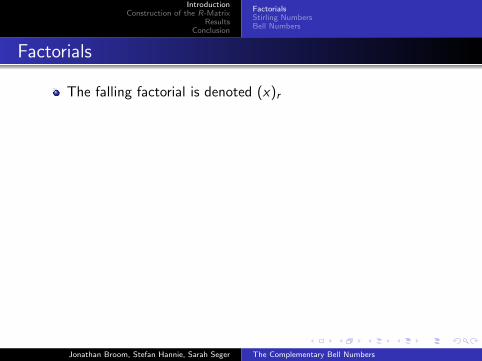
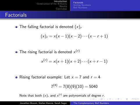
Factorials
The falling factorial is denoted (x)r
(x)r = x(x − 1)(x − 2) · · · (x − r + 1)
The rising factorial is denoted x (r)
x (r) = x(x + 1)(x + 2) · · · (x + r − 1)
Rising factorial example: Let x = 7 and r = 4
7(4) = 7(8)(9)(10) = 5040
Note that both (x)r and x (r) are polynomials of degree r .
Jonathan Broom, Stefan Hannie, Sarah Seger The Complementary Bell Numbers

IntroductionConstruction of the R-Matrix
ResultsConclusion
FactorialsStirling NumbersBell Numbers
Factorials
The falling factorial is denoted (x)r
(x)r = x(x − 1)(x − 2) · · · (x − r + 1)
The rising factorial is denoted x (r)
x (r) = x(x + 1)(x + 2) · · · (x + r − 1)
Rising factorial example: Let x = 7 and r = 4
7(4) = 7(8)(9)(10) = 5040
Note that both (x)r and x (r) are polynomials of degree r .
Jonathan Broom, Stefan Hannie, Sarah Seger The Complementary Bell Numbers

IntroductionConstruction of the R-Matrix
ResultsConclusion
FactorialsStirling NumbersBell Numbers
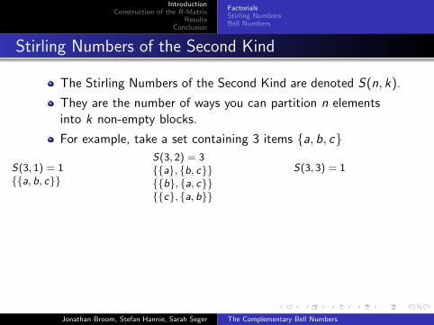
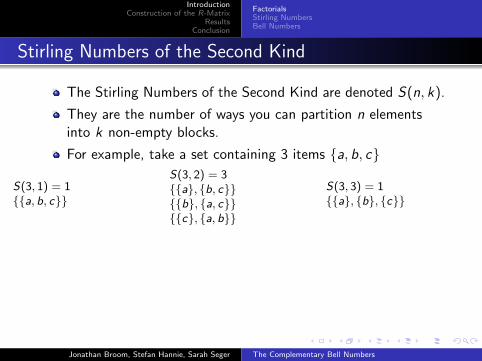
Stirling Numbers of the Second Kind
The Stirling Numbers of the Second Kind are denoted S(n, k).
They are the number of ways you can partition n elementsinto k non-empty blocks.
For example, take a set containing 3 items {a, b, c}
S(3, 1) = 1{{a, b, c}}
S(3, 2) = 3{{a}, {b, c}}{{b}, {a, c}}{{c}, {a, b}}
S(3, 3) = 1{{a}, {b}, {c}}
Another example for S(3, k):
Figure: S(3, 1) = 1 Figure: S(3, 2) = 3 Figure: S(3, 3) = 1
Jonathan Broom, Stefan Hannie, Sarah Seger The Complementary Bell Numbers

IntroductionConstruction of the R-Matrix
ResultsConclusion
FactorialsStirling NumbersBell Numbers
Stirling Numbers of the Second Kind
The Stirling Numbers of the Second Kind are denoted S(n, k).
They are the number of ways you can partition n elementsinto k non-empty blocks.
For example, take a set containing 3 items {a, b, c}
S(3, 1) = 1
{{a, b, c}}
S(3, 2) = 3{{a}, {b, c}}{{b}, {a, c}}{{c}, {a, b}}
S(3, 3) = 1{{a}, {b}, {c}}
Another example for S(3, k):
Figure: S(3, 1) = 1 Figure: S(3, 2) = 3 Figure: S(3, 3) = 1
Jonathan Broom, Stefan Hannie, Sarah Seger The Complementary Bell Numbers

IntroductionConstruction of the R-Matrix
ResultsConclusion
FactorialsStirling NumbersBell Numbers
Stirling Numbers of the Second Kind
The Stirling Numbers of the Second Kind are denoted S(n, k).
They are the number of ways you can partition n elementsinto k non-empty blocks.
For example, take a set containing 3 items {a, b, c}
S(3, 1) = 1{{a, b, c}}
S(3, 2) = 3{{a}, {b, c}}{{b}, {a, c}}{{c}, {a, b}}
S(3, 3) = 1{{a}, {b}, {c}}
Another example for S(3, k):
Figure: S(3, 1) = 1 Figure: S(3, 2) = 3 Figure: S(3, 3) = 1
Jonathan Broom, Stefan Hannie, Sarah Seger The Complementary Bell Numbers

IntroductionConstruction of the R-Matrix
ResultsConclusion
FactorialsStirling NumbersBell Numbers
Stirling Numbers of the Second Kind
The Stirling Numbers of the Second Kind are denoted S(n, k).
They are the number of ways you can partition n elementsinto k non-empty blocks.
For example, take a set containing 3 items {a, b, c}
S(3, 1) = 1{{a, b, c}}
S(3, 2) = 3
{{a}, {b, c}}{{b}, {a, c}}{{c}, {a, b}}
S(3, 3) = 1{{a}, {b}, {c}}
Another example for S(3, k):
Figure: S(3, 1) = 1 Figure: S(3, 2) = 3 Figure: S(3, 3) = 1
Jonathan Broom, Stefan Hannie, Sarah Seger The Complementary Bell Numbers

IntroductionConstruction of the R-Matrix
ResultsConclusion
FactorialsStirling NumbersBell Numbers
Stirling Numbers of the Second Kind
The Stirling Numbers of the Second Kind are denoted S(n, k).
They are the number of ways you can partition n elementsinto k non-empty blocks.
For example, take a set containing 3 items {a, b, c}
S(3, 1) = 1{{a, b, c}}
S(3, 2) = 3{{a}, {b, c}}
{{b}, {a, c}}{{c}, {a, b}}
S(3, 3) = 1{{a}, {b}, {c}}
Another example for S(3, k):
Figure: S(3, 1) = 1 Figure: S(3, 2) = 3 Figure: S(3, 3) = 1
Jonathan Broom, Stefan Hannie, Sarah Seger The Complementary Bell Numbers

IntroductionConstruction of the R-Matrix
ResultsConclusion
FactorialsStirling NumbersBell Numbers
Stirling Numbers of the Second Kind
The Stirling Numbers of the Second Kind are denoted S(n, k).
They are the number of ways you can partition n elementsinto k non-empty blocks.
For example, take a set containing 3 items {a, b, c}
S(3, 1) = 1{{a, b, c}}
S(3, 2) = 3{{a}, {b, c}}{{b}, {a, c}}
{{c}, {a, b}}
S(3, 3) = 1{{a}, {b}, {c}}
Another example for S(3, k):
Figure: S(3, 1) = 1 Figure: S(3, 2) = 3 Figure: S(3, 3) = 1
Jonathan Broom, Stefan Hannie, Sarah Seger The Complementary Bell Numbers

IntroductionConstruction of the R-Matrix
ResultsConclusion
FactorialsStirling NumbersBell Numbers
Stirling Numbers of the Second Kind
The Stirling Numbers of the Second Kind are denoted S(n, k).
They are the number of ways you can partition n elementsinto k non-empty blocks.
For example, take a set containing 3 items {a, b, c}
S(3, 1) = 1{{a, b, c}}
S(3, 2) = 3{{a}, {b, c}}{{b}, {a, c}}{{c}, {a, b}}
S(3, 3) = 1{{a}, {b}, {c}}
Another example for S(3, k):
Figure: S(3, 1) = 1 Figure: S(3, 2) = 3 Figure: S(3, 3) = 1
Jonathan Broom, Stefan Hannie, Sarah Seger The Complementary Bell Numbers
IntroductionConstruction of the R-Matrix
ResultsConclusion
FactorialsStirling NumbersBell Numbers
Stirling Numbers of the Second Kind
The Stirling Numbers of the Second Kind are denoted S(n, k).
They are the number of ways you can partition n elementsinto k non-empty blocks.
For example, take a set containing 3 items {a, b, c}
S(3, 1) = 1{{a, b, c}}
S(3, 2) = 3{{a}, {b, c}}{{b}, {a, c}}{{c}, {a, b}}
S(3, 3) = 1
{{a}, {b}, {c}}
Another example for S(3, k):
Figure: S(3, 1) = 1 Figure: S(3, 2) = 3 Figure: S(3, 3) = 1
Jonathan Broom, Stefan Hannie, Sarah Seger The Complementary Bell Numbers
IntroductionConstruction of the R-Matrix
ResultsConclusion
FactorialsStirling NumbersBell Numbers
Stirling Numbers of the Second Kind
The Stirling Numbers of the Second Kind are denoted S(n, k).
They are the number of ways you can partition n elementsinto k non-empty blocks.
For example, take a set containing 3 items {a, b, c}
S(3, 1) = 1{{a, b, c}}
S(3, 2) = 3{{a}, {b, c}}{{b}, {a, c}}{{c}, {a, b}}
S(3, 3) = 1{{a}, {b}, {c}}
Another example for S(3, k):
Figure: S(3, 1) = 1 Figure: S(3, 2) = 3 Figure: S(3, 3) = 1
Jonathan Broom, Stefan Hannie, Sarah Seger The Complementary Bell Numbers

IntroductionConstruction of the R-Matrix
ResultsConclusion
FactorialsStirling NumbersBell Numbers
Stirling Numbers of the Second Kind
The Stirling Numbers of the Second Kind are denoted S(n, k).
They are the number of ways you can partition n elementsinto k non-empty blocks.
For example, take a set containing 3 items {a, b, c}
S(3, 1) = 1{{a, b, c}}
S(3, 2) = 3{{a}, {b, c}}{{b}, {a, c}}{{c}, {a, b}}
S(3, 3) = 1{{a}, {b}, {c}}
Another example for S(3, k):
Figure: S(3, 1) = 1
Figure: S(3, 2) = 3 Figure: S(3, 3) = 1
Jonathan Broom, Stefan Hannie, Sarah Seger The Complementary Bell Numbers

IntroductionConstruction of the R-Matrix
ResultsConclusion
FactorialsStirling NumbersBell Numbers
Stirling Numbers of the Second Kind
The Stirling Numbers of the Second Kind are denoted S(n, k).
They are the number of ways you can partition n elementsinto k non-empty blocks.
For example, take a set containing 3 items {a, b, c}
S(3, 1) = 1{{a, b, c}}
S(3, 2) = 3{{a}, {b, c}}{{b}, {a, c}}{{c}, {a, b}}
S(3, 3) = 1{{a}, {b}, {c}}
Another example for S(3, k):
Figure: S(3, 1) = 1 Figure: S(3, 2) = 3
Figure: S(3, 3) = 1
Jonathan Broom, Stefan Hannie, Sarah Seger The Complementary Bell Numbers

IntroductionConstruction of the R-Matrix
ResultsConclusion
FactorialsStirling NumbersBell Numbers
Stirling Numbers of the Second Kind
The Stirling Numbers of the Second Kind are denoted S(n, k).
They are the number of ways you can partition n elementsinto k non-empty blocks.
For example, take a set containing 3 items {a, b, c}
S(3, 1) = 1{{a, b, c}}
S(3, 2) = 3{{a}, {b, c}}{{b}, {a, c}}{{c}, {a, b}}
S(3, 3) = 1{{a}, {b}, {c}}
Another example for S(3, k):
Figure: S(3, 1) = 1 Figure: S(3, 2) = 3 Figure: S(3, 3) = 1
Jonathan Broom, Stefan Hannie, Sarah Seger The Complementary Bell Numbers

IntroductionConstruction of the R-Matrix
ResultsConclusion
FactorialsStirling NumbersBell Numbers
Stirling Numbers of the Second Kind
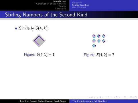
Similarly S(4, k):
Figure: S(4, 1) = 1 Figure: S(4, 2) = 7
Figure: S(4, 3) = 6 Figure: S(4, 4) = 1
Note: From the examples, it is clear that S(n, 1) = S(n, n) = 1.
Jonathan Broom, Stefan Hannie, Sarah Seger The Complementary Bell Numbers

IntroductionConstruction of the R-Matrix
ResultsConclusion
FactorialsStirling NumbersBell Numbers
Stirling Numbers of the Second Kind
Similarly S(4, k):
Figure: S(4, 1) = 1
Figure: S(4, 2) = 7
Figure: S(4, 3) = 6 Figure: S(4, 4) = 1
Note: From the examples, it is clear that S(n, 1) = S(n, n) = 1.
Jonathan Broom, Stefan Hannie, Sarah Seger The Complementary Bell Numbers
IntroductionConstruction of the R-Matrix
ResultsConclusion
FactorialsStirling NumbersBell Numbers
Stirling Numbers of the Second Kind
Similarly S(4, k):
Figure: S(4, 1) = 1 Figure: S(4, 2) = 7
Figure: S(4, 3) = 6 Figure: S(4, 4) = 1
Note: From the examples, it is clear that S(n, 1) = S(n, n) = 1.
Jonathan Broom, Stefan Hannie, Sarah Seger The Complementary Bell Numbers

IntroductionConstruction of the R-Matrix
ResultsConclusion
FactorialsStirling NumbersBell Numbers
Stirling Numbers of the Second Kind
Similarly S(4, k):
Figure: S(4, 1) = 1 Figure: S(4, 2) = 7
Figure: S(4, 3) = 6
Figure: S(4, 4) = 1
Note: From the examples, it is clear that S(n, 1) = S(n, n) = 1.
Jonathan Broom, Stefan Hannie, Sarah Seger The Complementary Bell Numbers

IntroductionConstruction of the R-Matrix
ResultsConclusion
FactorialsStirling NumbersBell Numbers
Stirling Numbers of the Second Kind
Similarly S(4, k):
Figure: S(4, 1) = 1 Figure: S(4, 2) = 7
Figure: S(4, 3) = 6 Figure: S(4, 4) = 1
Note: From the examples, it is clear that S(n, 1) = S(n, n) = 1.
Jonathan Broom, Stefan Hannie, Sarah Seger The Complementary Bell Numbers

IntroductionConstruction of the R-Matrix
ResultsConclusion
FactorialsStirling NumbersBell Numbers
Stirling Numbers of the Second Kind
Similarly S(4, k):
Figure: S(4, 1) = 1 Figure: S(4, 2) = 7
Figure: S(4, 3) = 6 Figure: S(4, 4) = 1
Note: From the examples, it is clear that S(n, 1) = S(n, n) = 1.
Jonathan Broom, Stefan Hannie, Sarah Seger The Complementary Bell Numbers

IntroductionConstruction of the R-Matrix
ResultsConclusion
FactorialsStirling NumbersBell Numbers
Growth
SH7, 4L = 350
SH6, 3L = 90
SH8, 4L = 1701
2 4 6 8k
500
1000
1500
SnHkL
The points labeled are the k values that yield the maximum S(n, k) for a given n.
Jonathan Broom, Stefan Hannie, Sarah Seger The Complementary Bell Numbers

IntroductionConstruction of the R-Matrix
ResultsConclusion
FactorialsStirling NumbersBell Numbers
Bell Numbers and Complementary Bell Numbers
The Bell Numbers are denoted B(n)
B(n) =n∑
k=1
S(n, k)
The Complementary Bell Numbers are denoted B̃(n)
B̃(n) =n∑
k=1
(−1)kS(n, k)
Jonathan Broom, Stefan Hannie, Sarah Seger The Complementary Bell Numbers
IntroductionConstruction of the R-Matrix
ResultsConclusion
FactorialsStirling NumbersBell Numbers
B̃(n) Examples
Examples:
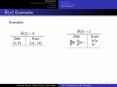
B̃(2) = 0
Odd Even{a, b} {a}, {b}
B̃(4) = 1
Odd Even
B̃(3) = 1
Odd Even
B̃(5) = −2
Odd Even
Jonathan Broom, Stefan Hannie, Sarah Seger The Complementary Bell Numbers

IntroductionConstruction of the R-Matrix
ResultsConclusion
FactorialsStirling NumbersBell Numbers
B̃(n) Examples
Examples:
B̃(2) = 0
Odd Even{a, b} {a}, {b}
B̃(4) = 1
Odd Even
B̃(3) = 1
Odd Even
B̃(5) = −2
Odd Even
Jonathan Broom, Stefan Hannie, Sarah Seger The Complementary Bell Numbers
IntroductionConstruction of the R-Matrix
ResultsConclusion
FactorialsStirling NumbersBell Numbers
B̃(n) Examples
Examples:
B̃(2) = 0
Odd Even{a, b} {a}, {b}
B̃(4) = 1
Odd Even
B̃(3) = 1
Odd Even
B̃(5) = −2
Odd Even
Jonathan Broom, Stefan Hannie, Sarah Seger The Complementary Bell Numbers

IntroductionConstruction of the R-Matrix
ResultsConclusion
FactorialsStirling NumbersBell Numbers
B̃(n) Examples
Examples:
B̃(2) = 0
Odd Even{a, b} {a}, {b}
B̃(4) = 1
Odd Even
B̃(3) = 1
Odd Even
B̃(5) = −2
Odd Even
Jonathan Broom, Stefan Hannie, Sarah Seger The Complementary Bell Numbers

IntroductionConstruction of the R-Matrix
ResultsConclusion
FactorialsStirling NumbersBell Numbers
B̃(n) Examples
Examples:
B̃(2) = 0
Odd Even{a, b} {a}, {b}
B̃(4) = 1
Odd Even
B̃(3) = 1
Odd Even
B̃(5) = −2
Odd Even
Jonathan Broom, Stefan Hannie, Sarah Seger The Complementary Bell Numbers

IntroductionConstruction of the R-Matrix
ResultsConclusion
FactorialsStirling NumbersBell Numbers
Complementary Bell Numbers
n B̃(n)0 11 −12 03 14 15 −26 −97 −98 509 267
10 41311 −218012 −1773113 −5053314 11017615 196679716 993866917 8638718...
...
æ æ
æ
æ æ
æ
æ æ
æ
2 4 6 8n
5
10
15
20
BnH-1L
Figure: |B̃(n)| for n ≤ 8Jonathan Broom, Stefan Hannie, Sarah Seger The Complementary Bell Numbers

IntroductionConstruction of the R-Matrix
ResultsConclusion
FactorialsStirling NumbersBell Numbers
Wilf’s Conjecture
H.S. Wilf’s Conjecture:
B̃(n) 6= 0 for all n > 2
Jonathan Broom, Stefan Hannie, Sarah Seger The Complementary Bell Numbers

IntroductionConstruction of the R-Matrix
ResultsConclusion
λj (x)BasisCoefficientsMatrices
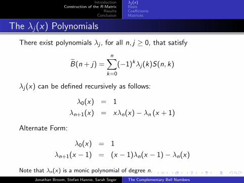
The λj(x) Polynomials
There exist polynomials λj , for all n, j ≥ 0, that satisfy
B̃(n + j) =n∑
k=0
(−1)kλj(k)S(n, k)
λj(x) can be defined recursively as follows:
λ0(x) = 1
λn+1(x) = xλn(x)− λn (x + 1)
Alternate Form:
λ0(x) = 1
λn+1(x − 1) = (x − 1)λn(x − 1)− λn(x)
Note that λn(x) is a monic polynomial of degree n.
Jonathan Broom, Stefan Hannie, Sarah Seger The Complementary Bell Numbers

IntroductionConstruction of the R-Matrix
ResultsConclusion
λj (x)BasisCoefficientsMatrices
The λj(x) Polynomials
There exist polynomials λj , for all n, j ≥ 0, that satisfy
B̃(n + j) =n∑
k=0
(−1)kλj(k)S(n, k)
λj(x) can be defined recursively as follows:
λ0(x) = 1
λn+1(x) = xλn(x)− λn (x + 1)
Alternate Form:
λ0(x) = 1
λn+1(x − 1) = (x − 1)λn(x − 1)− λn(x)
Note that λn(x) is a monic polynomial of degree n.
Jonathan Broom, Stefan Hannie, Sarah Seger The Complementary Bell Numbers
IntroductionConstruction of the R-Matrix
ResultsConclusion
λj (x)BasisCoefficientsMatrices
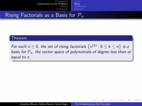
Rising Factorials as a Basis for Pn
Theorem
For each n ≥ 0, the set of rising factorials{
x (k) : 0 ≤ k ≤ n}
is abasis for Pn, the vector space of polynomials of degree less than orequal to n.
xn =n∑
k=0
(−1)n+kS(n, k)x (k) for all n ≥ 0
Jonathan Broom, Stefan Hannie, Sarah Seger The Complementary Bell Numbers

IntroductionConstruction of the R-Matrix
ResultsConclusion
λj (x)BasisCoefficientsMatrices
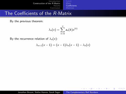
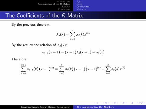
The Coefficients of the R-Matrix
By the previous theorem:
λn(x) =n∑
k=0
an(k)x(k)
By the recurrence relation of λn(x):
λn+1(x − 1) = (x − 1)λn(x − 1)− λn(x)
Therefore:
n+1∑k=0
an+1(k) (x − 1)(k) =n∑
k=0
an(k) (x − 1) (x − 1)(k) −n∑
k=0
an(k)x(k)
Lemma
For all n ≥ 0 and for all 0 ≤ k ≤ n + 1,
an+1(k)− (k + 1) an+1(k +1) = an(k − 1)− 2 (k + 1) an(k)+ (k + 1)2 an(k +1)
Jonathan Broom, Stefan Hannie, Sarah Seger The Complementary Bell Numbers
IntroductionConstruction of the R-Matrix
ResultsConclusion
λj (x)BasisCoefficientsMatrices
The Coefficients of the R-Matrix
By the previous theorem:
λn(x) =n∑
k=0
an(k)x(k)
By the recurrence relation of λn(x):
λn+1(x − 1) = (x − 1)λn(x − 1)− λn(x)
Therefore:
n+1∑k=0
an+1(k) (x − 1)(k) =n∑
k=0
an(k) (x − 1) (x − 1)(k) −n∑
k=0
an(k)x(k)
Lemma
For all n ≥ 0 and for all 0 ≤ k ≤ n + 1,
an+1(k)− (k + 1) an+1(k +1) = an(k − 1)− 2 (k + 1) an(k)+ (k + 1)2 an(k +1)
Jonathan Broom, Stefan Hannie, Sarah Seger The Complementary Bell Numbers

IntroductionConstruction of the R-Matrix
ResultsConclusion
λj (x)BasisCoefficientsMatrices
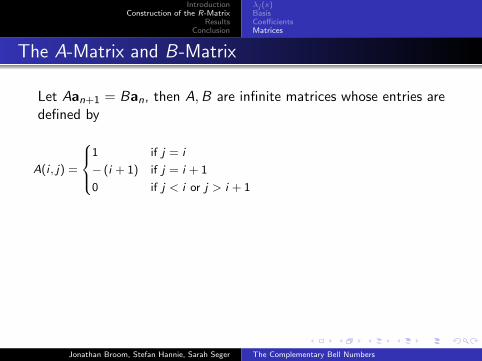
The A-Matrix and B-Matrix
Let Aan+1 = Ban, then A,B are infinite matrices whose entries aredefined by
A(i , j) =
1 if j = i
− (i + 1) if j = i + 1
0 if j < i or j > i + 1
B(i , j) =
1 if j = i − 1
−2 (i + 1) if j = i
(i + 1)2 if j = i + 1
0 if |i − j | > 1
A =
1 −1 0 0 . . .0 1 −2 0 . . .0 0 1 −3 . . .0 0 0 1 . . ....
......
.... . .
B =
−2 1 0 0 . . .1 −4 4 0 . . .0 1 −6 9 . . .0 0 1 −8 . . ....
......
.... . .
Jonathan Broom, Stefan Hannie, Sarah Seger The Complementary Bell Numbers
IntroductionConstruction of the R-Matrix
ResultsConclusion
λj (x)BasisCoefficientsMatrices
The A-Matrix and B-Matrix
Let Aan+1 = Ban, then A,B are infinite matrices whose entries aredefined by
A(i , j) =
1 if j = i
− (i + 1) if j = i + 1
0 if j < i or j > i + 1
B(i , j) =
1 if j = i − 1
−2 (i + 1) if j = i
(i + 1)2 if j = i + 1
0 if |i − j | > 1
A =
1 −1 0 0 . . .0 1 −2 0 . . .0 0 1 −3 . . .0 0 0 1 . . ....
......
.... . .
B =
−2 1 0 0 . . .1 −4 4 0 . . .0 1 −6 9 . . .0 0 1 −8 . . ....
......
.... . .
Jonathan Broom, Stefan Hannie, Sarah Seger The Complementary Bell Numbers
IntroductionConstruction of the R-Matrix
ResultsConclusion
λj (x)BasisCoefficientsMatrices
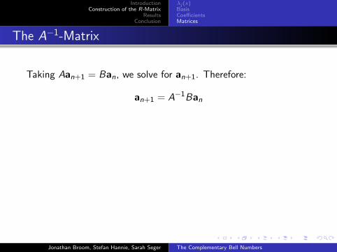
The A−1-Matrix
Taking Aan+1 = Ban, we solve for an+1. Therefore:
an+1 = A−1Ban
A−1(i , j) =
{j!i! if j ≥ i
0 if j < i A−1 =
1 1 2 6 24 . . .0 1 2 6 24 . . .0 0 1 3 12 . . .0 0 0 1 4 . . .0 0 0 0 1 . . ....
......
......
. . .
Jonathan Broom, Stefan Hannie, Sarah Seger The Complementary Bell Numbers

IntroductionConstruction of the R-Matrix
ResultsConclusion
λj (x)BasisCoefficientsMatrices
The A−1-Matrix
Taking Aan+1 = Ban, we solve for an+1. Therefore:
an+1 = A−1Ban
A−1(i , j) =
{j!i! if j ≥ i
0 if j < i
A−1 =
1 1 2 6 24 . . .0 1 2 6 24 . . .0 0 1 3 12 . . .0 0 0 1 4 . . .0 0 0 0 1 . . ....
......
......
. . .
Jonathan Broom, Stefan Hannie, Sarah Seger The Complementary Bell Numbers

IntroductionConstruction of the R-Matrix
ResultsConclusion
λj (x)BasisCoefficientsMatrices
The A−1-Matrix
Taking Aan+1 = Ban, we solve for an+1. Therefore:
an+1 = A−1Ban
A−1(i , j) =
{j!i! if j ≥ i
0 if j < i A−1 =
1 1 2 6 24 . . .0 1 2 6 24 . . .0 0 1 3 12 . . .0 0 0 1 4 . . .0 0 0 0 1 . . ....
......
......
. . .
Jonathan Broom, Stefan Hannie, Sarah Seger The Complementary Bell Numbers

IntroductionConstruction of the R-Matrix
ResultsConclusion
λj (x)BasisCoefficientsMatrices
The R-Matrix
Taking an+1 = A−1Ban, we call R = A−1B. Therefore:
an+1 = Ran
R(i , j) =
− j!
i! if j > i
−(i + 1) if j = i
1 if j = i − 1
0 if j < i − 1
R =
−1 −1 −2 −6 −24 . . .1 −2 −2 −6 −24 . . .0 1 −3 −3 −12 . . .0 0 1 −4 −4 . . .0 0 0 1 −5 . . ....
......
......
. . .
Jonathan Broom, Stefan Hannie, Sarah Seger The Complementary Bell Numbers

IntroductionConstruction of the R-Matrix
ResultsConclusion
Infinite MatricesFinite Matrices
The Lower Section
Lemma
For each n ∈ N, the nth power of R is defined and Rn(i , j) = 0 ifj < i − n.
R =
−1 −1 −2 −6 −24 . . .1 −2 −2 −6 −24 . . .0 1 −3 −3 −12 . . .0 0 1 −4 −4 . . .0 0 0 1 −5 . . .
.
.
.
.
.
.
.
.
.
.
.
.
.
.
.. . .
R2 =
0 1 4 18 96 . . .−3 1 2 12 72 . . .
1 −5 4 3 24 . . .0 1 −7 9 4 . . .0 0 1 −9 16 . . .
.
.
.
.
.
.
.
.
.
.
.
.
.
.
.. . .
R3 =
1 2 4 6 −24 . . .4 3 10 30 96 . . .
−6 13 −1 24 96 . . .1 −9 28 −17 44 . . .0 1 −12 49 −51 . . .
.
.
.
.
.
.
.
.
.
.
.
.
.
.
.. . .
R4 =
1 −1 −12 −78 −504 . . .−1 0 −14 −96 −648 . . .19 −21 13 −39 −312 . . .
−10 45 −85 76 −76 . . .1 −14 83 −217 249 . . .
.
.
.
.
.
.
.
.
.
.
.
.
.
.
.. . .
Jonathan Broom, Stefan Hannie, Sarah Seger The Complementary Bell Numbers

IntroductionConstruction of the R-Matrix
ResultsConclusion
Infinite MatricesFinite Matrices
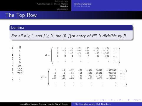
The Top Row
Lemma
For all n ≥ 1 and j ≥ 0, the (0, j)th entry of Rn is divisible by j!.
j j!0 11 12 23 64 245 1206 720...
...
R =
−1 −1 −2 −6 −24 −120 −720 . . .1 −2 −2 −6 −24 −120 −720 . . .0 1 −3 −3 −12 −60 −360 . . .0 0 1 −4 −4 −20 −120 . . .
.
.
.
.
.
.
.
.
.
.
.
.
.
.
.
.
.
.
.
.
.. . .
R4 =
1 −1 −12 −78 −504 36840 −953280 . . .−1 0 −14 −96 −648 35640 −923760 . . .19 −21 13 −39 −312 17700 −443880 . . .
−10 45 −85 76 −76 6000 −141000 . . .
.
.
.
.
.
.
.
.
.
.
.
.
.
.
.
.
.
.
.
.
.. . .
For R4: −783!
= −13, −5044!
= −21, 368405!
= 307, −9532806!
= −1324
Jonathan Broom, Stefan Hannie, Sarah Seger The Complementary Bell Numbers

IntroductionConstruction of the R-Matrix
ResultsConclusion
Infinite MatricesFinite Matrices
The Top Row
Lemma
For all n ≥ 1 and j ≥ 0, the (0, j)th entry of Rn is divisible by j!.
j j!0 11 12 23 64 245 1206 720...
...
R =
−1 −1 −2 −6 −24 −120 −720 . . .1 −2 −2 −6 −24 −120 −720 . . .0 1 −3 −3 −12 −60 −360 . . .0 0 1 −4 −4 −20 −120 . . .
.
.
.
.
.
.
.
.
.
.
.
.
.
.
.
.
.
.
.
.
.. . .
R4 =
1 −1 −12 −78 −504 36840 −953280 . . .−1 0 −14 −96 −648 35640 −923760 . . .19 −21 13 −39 −312 17700 −443880 . . .
−10 45 −85 76 −76 6000 −141000 . . .
.
.
.
.
.
.
.
.
.
.
.
.
.
.
.
.
.
.
.
.
.. . .
For R4: −783!
= −13, −5044!
= −21, 368405!
= 307, −9532806!
= −1324
Jonathan Broom, Stefan Hannie, Sarah Seger The Complementary Bell Numbers
IntroductionConstruction of the R-Matrix
ResultsConclusion
Infinite MatricesFinite Matrices
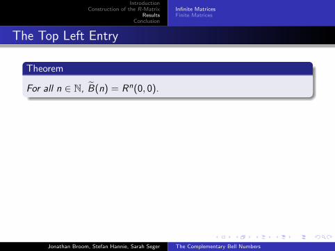
The Top Left Entry
Theorem
For all n ∈ N, B̃(n) = Rn(0, 0).
n B̃(n)1 −12 03 14 15 −26 −9...
...
R =
−1 −1 −2 −6 . . .1 −2 −2 −6 . . .0 1 −3 −3 . . .0 0 1 −4 . . .
.
.
.
.
.
.
.
.
.
.
.
.. . .
R5 =
−2 −11 −42 −156 . . .1 −13 −52 −216 . . .
−40 36 −74 −183 . . .55 −165 261 −335 . . .
.
.
.
.
.
.
.
.
.
.
.
.. . .
R2 =
0 1 4 18 . . .−3 1 2 12 . . .
1 −5 4 3 . . .0 1 −7 9 . . .
.
.
.
.
.
.
.
.
.
.
.
.. . .
R6 =
−9 −18 −4 40644 . . .−14 −27 −36 40548 . . .
76 −106 47 20286 . . .−220 536 −898 7473 . . .
.
.
.
.
.
.
.
.
.
.
.
.. . .
Jonathan Broom, Stefan Hannie, Sarah Seger The Complementary Bell Numbers

IntroductionConstruction of the R-Matrix
ResultsConclusion
Infinite MatricesFinite Matrices
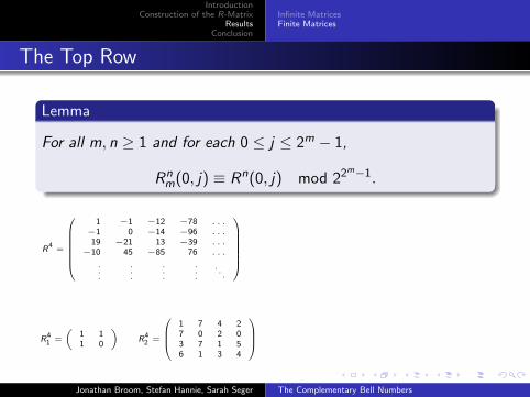
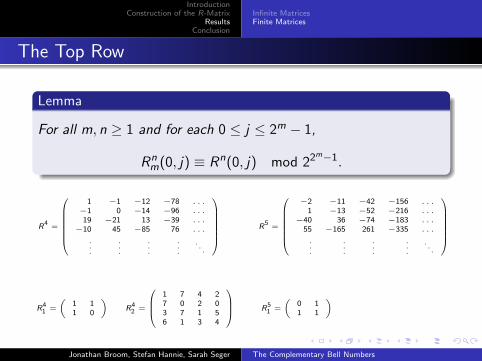
The Top Row
Lemma
For all m, n ≥ 1 and for each 0 ≤ j ≤ 2m − 1,
Rnm(0, j) ≡ Rn(0, j) mod 22m−1.
R4 =
1 −1 −12 −78 . . .−1 0 −14 −96 . . .19 −21 13 −39 . . .
−10 45 −85 76 . . .
.
.
.
.
.
.
.
.
.
.
.
.. . .
R41 =
(1 11 0
)R4
2 =
1 7 4 27 0 2 03 7 1 56 1 3 4
R5 =
−2 −11 −42 −156 . . .1 −13 −52 −216 . . .
−40 36 −74 −183 . . .55 −165 261 −335 . . .
.
.
.
.
.
.
.
.
.
.
.
.. . .
R51 =
(0 11 1
)R5
2 =
6 5 6 41 3 4 04 0 6 53 3 5 5
Jonathan Broom, Stefan Hannie, Sarah Seger The Complementary Bell Numbers

IntroductionConstruction of the R-Matrix
ResultsConclusion
Infinite MatricesFinite Matrices
The Top Row
Lemma
For all m, n ≥ 1 and for each 0 ≤ j ≤ 2m − 1,
Rnm(0, j) ≡ Rn(0, j) mod 22m−1.
R4 =
1 −1 −12 −78 . . .−1 0 −14 −96 . . .19 −21 13 −39 . . .
−10 45 −85 76 . . .
.
.
.
.
.
.
.
.
.
.
.
.. . .
R41 =
(1 11 0
)
R42 =
1 7 4 27 0 2 03 7 1 56 1 3 4
R5 =
−2 −11 −42 −156 . . .1 −13 −52 −216 . . .
−40 36 −74 −183 . . .55 −165 261 −335 . . .
.
.
.
.
.
.
.
.
.
.
.
.. . .
R51 =
(0 11 1
)R5
2 =
6 5 6 41 3 4 04 0 6 53 3 5 5
Jonathan Broom, Stefan Hannie, Sarah Seger The Complementary Bell Numbers
IntroductionConstruction of the R-Matrix
ResultsConclusion
Infinite MatricesFinite Matrices
The Top Row
Lemma
For all m, n ≥ 1 and for each 0 ≤ j ≤ 2m − 1,
Rnm(0, j) ≡ Rn(0, j) mod 22m−1.
R4 =
1 −1 −12 −78 . . .−1 0 −14 −96 . . .19 −21 13 −39 . . .
−10 45 −85 76 . . .
.
.
.
.
.
.
.
.
.
.
.
.. . .
R41 =
(1 11 0
)R4
2 =
1 7 4 27 0 2 03 7 1 56 1 3 4
R5 =
−2 −11 −42 −156 . . .1 −13 −52 −216 . . .
−40 36 −74 −183 . . .55 −165 261 −335 . . .
.
.
.
.
.
.
.
.
.
.
.
.. . .
R51 =
(0 11 1
)R5
2 =
6 5 6 41 3 4 04 0 6 53 3 5 5
Jonathan Broom, Stefan Hannie, Sarah Seger The Complementary Bell Numbers

IntroductionConstruction of the R-Matrix
ResultsConclusion
Infinite MatricesFinite Matrices
The Top Row
Lemma
For all m, n ≥ 1 and for each 0 ≤ j ≤ 2m − 1,
Rnm(0, j) ≡ Rn(0, j) mod 22m−1.
R4 =
1 −1 −12 −78 . . .−1 0 −14 −96 . . .19 −21 13 −39 . . .
−10 45 −85 76 . . .
.
.
.
.
.
.
.
.
.
.
.
.. . .
R41 =
(1 11 0
)R4
2 =
1 7 4 27 0 2 03 7 1 56 1 3 4
R5 =
−2 −11 −42 −156 . . .1 −13 −52 −216 . . .
−40 36 −74 −183 . . .55 −165 261 −335 . . .
.
.
.
.
.
.
.
.
.
.
.
.. . .
R51 =
(0 11 1
)R5
2 =
6 5 6 41 3 4 04 0 6 53 3 5 5
Jonathan Broom, Stefan Hannie, Sarah Seger The Complementary Bell Numbers
IntroductionConstruction of the R-Matrix
ResultsConclusion
Infinite MatricesFinite Matrices
The Top Row
Lemma
For all m, n ≥ 1 and for each 0 ≤ j ≤ 2m − 1,
Rnm(0, j) ≡ Rn(0, j) mod 22m−1.
R4 =
1 −1 −12 −78 . . .−1 0 −14 −96 . . .19 −21 13 −39 . . .
−10 45 −85 76 . . .
.
.
.
.
.
.
.
.
.
.
.
.. . .
R41 =
(1 11 0
)R4
2 =
1 7 4 27 0 2 03 7 1 56 1 3 4
R5 =
−2 −11 −42 −156 . . .1 −13 −52 −216 . . .
−40 36 −74 −183 . . .55 −165 261 −335 . . .
.
.
.
.
.
.
.
.
.
.
.
.. . .
R51 =
(0 11 1
)
R52 =
6 5 6 41 3 4 04 0 6 53 3 5 5
Jonathan Broom, Stefan Hannie, Sarah Seger The Complementary Bell Numbers

IntroductionConstruction of the R-Matrix
ResultsConclusion
Infinite MatricesFinite Matrices
The Top Row
Lemma
For all m, n ≥ 1 and for each 0 ≤ j ≤ 2m − 1,
Rnm(0, j) ≡ Rn(0, j) mod 22m−1.
R4 =
1 −1 −12 −78 . . .−1 0 −14 −96 . . .19 −21 13 −39 . . .
−10 45 −85 76 . . .
.
.
.
.
.
.
.
.
.
.
.
.. . .
R41 =
(1 11 0
)R4
2 =
1 7 4 27 0 2 03 7 1 56 1 3 4
R5 =
−2 −11 −42 −156 . . .1 −13 −52 −216 . . .
−40 36 −74 −183 . . .55 −165 261 −335 . . .
.
.
.
.
.
.
.
.
.
.
.
.. . .
R51 =
(0 11 1
)R5
2 =
6 5 6 41 3 4 04 0 6 53 3 5 5
Jonathan Broom, Stefan Hannie, Sarah Seger The Complementary Bell Numbers

IntroductionConstruction of the R-Matrix
ResultsConclusion
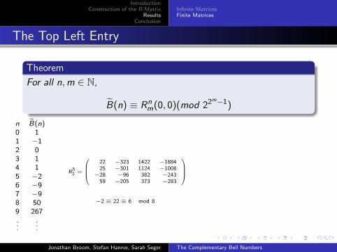
Infinite MatricesFinite Matrices
The Top Left Entry
Theorem
For all n,m ∈ N,
B̃(n) ≡ Rnm(0, 0)(mod 22m−1)
n B̃(n)0 11 −12 03 14 15 −26 −97 −98 509 267...
...
R52 =
22 −323 1422 −188425 −301 1124 −1008
−28 −96 382 −24359 −205 373 −283
−2 ≡ 22 ≡ 6 mod 8
R92 =
46203 −112360 161308 −13968631762 −66157 80710 −76050
9756 −18293 24253 −3675010181 −20787 33462 −30421
267 ≡ 46203 ≡ 3 mod 8
Jonathan Broom, Stefan Hannie, Sarah Seger The Complementary Bell Numbers

IntroductionConstruction of the R-Matrix
ResultsConclusion
Infinite MatricesFinite Matrices
The Top Left Entry
Theorem
For all n,m ∈ N,
B̃(n) ≡ Rnm(0, 0)(mod 22m−1)
n B̃(n)0 11 −12 03 14 15 −26 −97 −98 509 267...
...
R52 =
22 −323 1422 −188425 −301 1124 −1008
−28 −96 382 −24359 −205 373 −283
−2 ≡ 22 ≡ 6 mod 8
R92 =
46203 −112360 161308 −13968631762 −66157 80710 −76050
9756 −18293 24253 −3675010181 −20787 33462 −30421
267 ≡ 46203 ≡ 3 mod 8
Jonathan Broom, Stefan Hannie, Sarah Seger The Complementary Bell Numbers

IntroductionConstruction of the R-Matrix
ResultsConclusion
ConclusionAcknowledgementsWorks Cited
Conclusion
In Conclusion:
Additional Results
Alternate Bases
Jonathan Broom, Stefan Hannie, Sarah Seger The Complementary Bell Numbers

IntroductionConstruction of the R-Matrix
ResultsConclusion
ConclusionAcknowledgementsWorks Cited
Conclusion
In Conclusion:
Additional Results
Alternate Bases
Jonathan Broom, Stefan Hannie, Sarah Seger The Complementary Bell Numbers
IntroductionConstruction of the R-Matrix
ResultsConclusion
ConclusionAcknowledgementsWorks Cited
Conclusion
In Conclusion:
Additional Results
Alternate Bases
Jonathan Broom, Stefan Hannie, Sarah Seger The Complementary Bell Numbers

IntroductionConstruction of the R-Matrix
ResultsConclusion
ConclusionAcknowledgementsWorks Cited
Acknowledgements
We would like to thank LSU for hosting the SMILE Program.Thank you NSF for funding the VIGRE program. Thank you to Dr.De Angelis for spending his summer with us. Thank you to SimonPfeil for mentoring us.
Jonathan Broom, Stefan Hannie, Sarah Seger The Complementary Bell Numbers

IntroductionConstruction of the R-Matrix
ResultsConclusion
ConclusionAcknowledgementsWorks Cited
Works Cited
T. Amdeberhan, V. De Angelis, and V.H. Moll.Complementary Bell Numbers: Arithmetical Properties andWilf’s Conjecture. 2011.
http://www-history.mcs.st-and.ac.uk/Miscellaneous/StirlingBell/stirling2.html
Jonathan Broom, Stefan Hannie, Sarah Seger The Complementary Bell Numbers