the community reinvestment act and its effect on - cohnreznick
TRANSCRIPT

The Community Reinvestment Act and Its Effect on Housing Tax Credit Pricing
A Corresponding Analysis to CohnReznick’s Report The Low-Income Housing Tax Credit Program at Year 25: An Expanded Look at Its Performance

CohnReznick gathered information from the Federal Deposit Insurance Corporation’s (FDIC’s) website to obtain the address of every branch location for the top 20 commercial banks and used information gathered from the housing credit industry participants listed in Appendix A to compile this study. The information provided to us has not been indepen-dently tested or verified. As a result, we have relied exclusively on the study participants for the accuracy and completeness of their data. No study can be guaranteed to be 100% accurate, and errors can occur. CohnReznick does not warrant the completeness or the accuracy of the data submitted by study participants and thus does not accept responsibility for your reliance on this report or any of the information contained herein. The information contained in this report includes estimations, approximations and assump-tions and is not intended to be legal, accounting or tax advice. Please consult a lawyer, accountant or tax advisor before relying on any information contained in this report. CohnReznick disclaims any liability associated with your reliance on any information contained herein.
To ensure compliance with the requirements imposed by the IRS, we inform you that any U.S. federal tax advice contained in this communication (including any attachments) is not intended or written to be used, and cannot be used, for the purpose of (i) avoiding penal-ties under the Internal Revenue Code or (ii) promoting, marketing or recommending to another party any transaction or matter addressed herein.
Report Restrictions

A CohnReznick Report | 1
Table of Contents
Introduction . . . . . . . . . . . . . . . . . . . . . . . . . . . . . . . . . . . . . . . . . . . . . . . . . . . . . . . . . 3
Chapter 1: Executive Summary . . . . . . . . . . . . . . . . . . . . . . . . . . . . . . . . . . . . . . 5
Chapter 2: Background: The CRA and the Housing Tax Credit Program . . . . . . . . . . . . . . . . . . . . . . . . . . . . . 10
2.1: Overview . . . . . . . . . . . . . . . . . . . . . . . . . . . . . . . . . . . . . . . . 10
2.2: The Beginning of the CRA . . . . . . . . . . . . . . . . . . . . . . . . . 10
2.3: The Evolution of the CRA . . . . . . . . . . . . . . . . . . . . . . . . . . 12
2.4: A Synergistic Relationship: The CRA and the Housing Tax Credit Program . . . . . . . . . . . . . . . 14
2.5: The Geographic Mismatch . . . . . . . . . . . . . . . . . . . . . . . . 15
Chapter 3: Study Methodology . . . . . . . . . . . . . . . . . . . . . . . . . . . . . . . . . . . . 19
Chapter 4: Findings: The Impact of the CRA on the Housing Tax Credit Program . . . . . . . . . . . . . . . . . . . . . . 26
4.1: CRA Impact on the Availability of Housing Tax Credit Equity . . . . . . . . . . . . . . . . . . . . . . . 26
4.2: How Much Is a Dollar of Housing Tax Credit Worth? . . . . . . . . . . . . . . . . . . . . . . . . 27
4.3: State-Level Housing Tax Credit Pricing Analysis . . . . . . . . . . . . . . . . . . . . . . . . . . . . . . . . . . . 31
4.4: Individual Market Housing Tax Credit Pricing Analysis . . . . . . . . . . . . . . . . . . . . . . . . . 35
4.5: Are There Any Factors That Drive Pricing More Than the CRA? . . . . . . . . . . . . . . . . . . . . . . 45
Appendices: . . . . . . . . . . . . . . . . . . . . . . . . . . . . . . . . . . . . . . . . . . . . . . . . . . . . . . . 48
Appendix A: Acknowledgements. . . . . . . . . . . . . . . . . . . . . . . . 48
Appendix B: Surveyed Property Distribution by State and by CRA Heat Zone . . . . . . . . . . . . . . . . . . . . . 49
Appendix C: Distribution of Heat Map-Coded Zip Codes by State . . . . . . . . . . . . . . . . . . . . . . . . . 51

| The Community Reinvestment Act2
FiguRe 2.2(A) Philadelphia Federal Home Loan Bank Board Map – 1934 . . . . . . . . . 11FiguRe 2.2(B) Post CRA — Surveyed Housing Tax Credit Property Locations
on Philadelphia FHLBB Map . . . . . . . . . . . . . . . . . . . . . . . . . . . . . . . 12FiguRe 2.4.1 Asset Concentrations among U.S. Banks . . . . . . . . . . . . . . . . . . . . . . 15FiguRe 2.4.2(A) Percentage of CRA Ratings — All Banks . . . . . . . . . . . . . . . . . . . . . . 16FiguRe 2.4.2(B) Percentage of CRA Ratings — Top 20 Banks . . . . . . . . . . . . . . . . . . . 16FiguRe 3.1 Top 20 U.S.-Based Commercial Banks . . . . . . . . . . . . . . . . . . . . . . . . 20FiguRe 3.2 Heat Map Key . . . . . . . . . . . . . . . . . . . . . . . . . . . . . . . . . . . . . . . . . 22FiguRe 3.3 National CRA Heat Map . . . . . . . . . . . . . . . . . . . . . . . . . . . . . . . . . . 23FiguRe 4.1.1 Surveyed Properties on CRA Heat Map . . . . . . . . . . . . . . . . . . . . . . . 26FiguRe 4.1.2 Surveyed Property Distribution by Heat Zone . . . . . . . . . . . . . . . . . . . 27FiguRe 4.2.1 Housing Tax Credit Pricing Trend for Selected MSAs (2006–2008) . . . . . 29FiguRe 4.2.2 2008 Median Housing Tax Credit Pricing for Selected MSAs . . . . . . . . 30FiguRe 4.3.1 2005–2007 Statewide Median Housing Tax Credit Pricing . . . . . . . . . . 32FiguRe 4.3.2 2005–2007 Top 5 and Bottom 5 Statewide
Median Housing Tax Credit Pricing . . . . . . . . . . . . . . . . . . . . . . . . . . 33FiguRe 4.3.3 2006: Regulators Incentivize Investment:
Louisiana vs. National Median Tax Credit Pricing . . . . . . . . . . . . . . . . 34FiguRe 4.3.4 Statewide Housing Tax Credit Pricing Trend by Time Period. . . . . . . . . 34FiguRe 4.4.1(A) Operating Performance: National, Indiana
and Indianapolis MSA . . . . . . . . . . . . . . . . . . . . . . . . . . . . . . . . . . . . 36FiguRe 4.4.1(B) CRA Heat Map of Indiana with Surveyed Properties . . . . . . . . . . . . . . 37FiguRe 4.4.1(C) CRA Heat Map of Indianapolis with Surveyed Properties . . . . . . . . . . 38FiguRe 4.4.1(D) Indiana vs. Indianapolis Housing Tax Credit Pricing by CRA Zone . . . . 38FiguRe 4.4.2(A) Operating Performance: National, Arkansas
and Little Rock MSA . . . . . . . . . . . . . . . . . . . . . . . . . . . . . . . . . . . . . 39FiguRe 4.4.2(B) CRA Heat Map of Arkansas with Surveyed Properties . . . . . . . . . . . . . 40FiguRe 4.4.2(C) CRA Heat Map of Little Rock with Surveyed Properties . . . . . . . . . . . . 41FiguRe 4.4.2(D) Arkansas vs. Little Rock Housing Tax Credit Pricing by CRA Zone . . . . . 41FiguRe 4.4.3(A) Operating Performance: National, California
and San Diego MSA . . . . . . . . . . . . . . . . . . . . . . . . . . . . . . . . . . . . . 42FiguRe 4.4.3(B) CRA Heat Map of California with Surveyed Properties . . . . . . . . . . . . 43FiguRe 4.4.3(C) CRA Heat Map of San Diego with Surveyed Properties. . . . . . . . . . . . 44FiguRe 4.4.3(D) California vs. San Diego Housing Tax Credit Pricing by CRA Zone . . . . 44
Index of Figures

A CohnReznick Report | 3
The housing tax credit industry’s worst-kept secret is the relationship between the
Community Reinvestment Act (CRA) and the price of housing credit capital. The CRA, a federal banking statute initially enacted to reverse decades of disinvestment in our nation’s urban centers, ensures that banks that accept monetary deposits in distressed neighborhoods are also meeting the investment and borrowing needs
of those neighborhoods. The Low-Income Housing Tax Credit Program (housing tax credit), established in Section 42 of the Internal Revenue Code, was designed to stimulate the production of affordable housing in the United States—and has been undoubtedly successful at doing so. In fact, a great synergy has developed between the CRA and the housing tax credit program; while the latter program spurs the development of affordable housing projects, the former acts as a source of capital formation for many of those very projects.
Since the mid-1990s, the equity market for housing tax credit investments has been predominantly composed of large, publicly traded companies, most of which are in the banking and financial services sector. CohnReznick estimates that approximately $10 billion of capital was committed to housing tax credit investments in 2012, and that the banking sector was the source for approximately 85% of that amount.1 U.S. banks were among the first corporate investors in housing credit projects and have seen their market share in these investments grow steadily to a level where it currently represents the life blood of the housing tax credit equity market.
Why are housing credit investments so attractive to banks? There are a number of reasons:
• The housing tax credit is earned over a 15-year period but is claimed over an acceler-ated 10-year timeframe, beginning in the year in which the property is placed in service and units are occupied. The ideal housing credit investor is a company with a track record of consistent growth in earnings and is a “regular” federal taxpayer. This has been the profile of the U.S. banking industry for 24 of the last 26 years.
• When bank investors were surveyed about why they were so attracted to housing credit investments, they responded that their principal motivation for making such investments was to help meet their obligation to comply with the CRA.2 Banks are obligated, under the CRA regulations, to make loans, provide services and make investments in low- to moderate-income neighborhoods in those areas within which they conduct business. There are a limited number of qualified equity investments under CRA regulations, and many of these have unattractive yield and/or risk profiles. Among the available invest-ment options, housing credit investments appear to be the clear investor favorite.
Introduction
1 This estimate is largely based on data collected during an industry survey CohnReznick conducted in January 2013, adjusted based on anecdotal evidence.
2 Source: Ernst & Young. “Low Income Housing Tax Credit Investment Survey – October 2009,” page 5.

| The Community Reinvestment Act4
• Surveyed banks also cited that on a risk-adjusted basis, the yields of housing credit invest-ments are superior to many available alternatives. This is, in part, because banks enjoy a lower cost of funds than other investors, which widens the spread between that cost and the rate of return offered by housing credit investments.
While the Community Reinvestment Act has been an enormously successful vehicle for assembling capital for the development of affordable housing, criticism has been leveled at the fact that much of the banking sector’s demand for housing credit investment is disproportionately focused in parts of the country where bank deposits—and conse-quently, bank appetite for CRA eligible investments—are the highest.
The CRA has been the subject of studies over the years by academics, think tanks and government agencies. Many of these studies focused on CRA-regulated loans versus equity investments. In fact, to the best of our knowledge, no previous study has analyzed the impact the CRA has had on the availability and price of housing tax credit equity capital. CohnReznick has undertaken this pioneering study with the goal of filling this knowl-edge gap and providing food for thought. As a result of this study, CohnReznick arrived at the conclusion that, while the success of the CRA and housing tax credit program, and the synergy between the two cannot be denied, the spread in housing tax credit prices between projects in CRA-hot versus CRA-not markets suggests that a new approach to how CRA assessment areas are defined may be in order.3
3 CohnReznick has become accustomed to referring to areas with high CRA value as “CRA-hot” and areas with limited CRA value as “CRA-not.”

A CohnReznick Report | 5
ChApteR 1:
Executive Summary
The Community Reinvestment Act has been a great engine of capital formation for developing affordable housing in the United States. The
affordable housing industry would not be the same without the synergy between the CRA and the housing tax credit program. As investors and regulators have become increasingly confident in the financial performance of housing tax credit properties as an asset class, the housing tax credit program has become more reliant on the banking sector, as a highly reliable source of equity, to meet its capital needs. This has been a largely favorable development because banks, for example, filled most of the equity gap created when Fannie Mae and Freddie Mac exited the housing credit market in 2007 and 2008. In fact, according to CohnReznick’s data and analysis approximately 76% of the surveyed housing tax credit properties are located in areas where at least one of the top 20 u.S. commercial banks has CRA responsibility.
In theory, a dollar of housing tax credit should be worth a dollar, whether the tax credit is generated by a project located in Martinsville, West Virginia, or downtown San Francisco, California. As a practical matter, however, housing credit investors must acquire tax credits at a discount from a dollar to achieve a return on their capital and some level of invest-ment yield on that capital. The magnitude of the discount is a function of several factors that ultimately determine the “cost” of housing credit equity.
| The Community Reinvestment Act6
Our study reveals several findings:
•We posit that the largest single determinant of housing tax credit pricing is based on the CRA investment test value of a given property’s location. By “CRA investment test value” we refer to the fact that a housing tax credit project located within a bank’s CRA footprint will receive positive consideration in determining whether a bank has met its CRA investment test objectives. The investment test is one of the three tests by which large banks are evaluated for CRA performance, the other two being the lending and service tests.4 The data CohnReznick collected clearly indicate large pricing spreads—as wide as $0.35 per $1.00 of housing tax credit at the extreme ends of the pricing spectrum between CRA-hot and CRA-not locations—which cannot be explained sufficiently by factors other than the CRA.
•Notwithstanding the synergy that has developed between the CRA and the housing tax credit program, it is clear that there is a mismatch between the factors that drive investment test objectives and the manner in which housing credits are allocated. The allocation of housing credits is principally driven by each state’s assessment of its most critical housing needs. The banking sector’s demand for housing credit investment is disproportionately focused in parts of the country where bank deposits—and conse-quently, investment test requirements—are the highest. Therefore, the banking sector’s demand for housing credit investment is not proportionately aligned with the location of housing credit properties. This has led to a phenomenon of overlapping CRA assessment areas in highly populated markets. As a result, the investment test tends to drive capital to highly competitive areas that may result in a disproportionately small number of avail-able investment opportunities, as measured by population and/or deposits. Competition for housing tax credit investments in areas with limited investment opportunities tends to create a massive supply/demand imbalance.
• in general, housing tax credit prices have increased while yields have trended down-wardovertimeasinvestorshavebecomemoreconfidentintherisk/rewardprofileofhousing tax credit investments. That said, another major determinant of pricing is the equity demand for housing credit investments at a particular point in time. Thus, when the equity market was at its historical peak volume in 2006, housing tax credits were trading more or less at par ($1 for $1) in many locations. It is within this period that we observed, from data collected in this study, the narrowest ($0.14) spread between states with the highest and most concentrated CRA demand and those with the least. By contrast, when economic conditions in the U.S. and around the globe deteriorated in 2008-2009 and taxable incomes against which tax credits are applied decreased, investor demand necessitated significantly lower tax credit pricing. In CRA-hot areas of the country, however, even during the bottom of the equity market, demand for housing credit investments and housing tax credit prices were affected by a much smaller magnitude. the most sought-after CRA markets had the strongest resistance to steep decreases in tax credit prices, even in the midst of market uncertainty.
4 Large banks are currently defined as those having assets of $1.186 billion or more for December 31 of both of the past two years, effective January 1, 2013. Source: http://www.ffiec.gov/cra/examinations.htm.

A CohnReznick Report | 7
Further, given the fact that CRA-motivated banks were virtually the sole source of housing tax credit equity during the recent economic downturn, much steeper differ-ences in price were observed between CRA-hot and CRA-not markets. During this period, a $0.24 spread was observed between some states. If not for the Tax Credit Exchange Program and the Tax Credit Assistance Program, we would have expected this spread to be even wider.5
CohnReznick concludes that all else remaining constant, the more the market is domi-nated by CRA-motivated investors who invest only in certain areas of the country, the wider the pricing spread one may expect to see between areas with intense CRA compliance demand and areas without.
Since CRA-motivated banks represented virtually the sole source of equity during the recent economic downturn, two interesting trends in pricing developed:
» In the most highly sought after markets for housing credit investment, (San Francisco, New York, Los Angeles, etc.) housing tax credit prices decreased but by a very modest level. Median pricing in CRA-hot markets was just under $1.00.
» By contrast, median pricing in smaller metropolitan areas like Indianapolis and Milwaukee decreased by substantial levels to $0.68. Median tax credit prices in micropolitan and rural areas were as low as $0.60, turning financially feasible projects into deals that simply did not “pencil out.”6 As indicated previously, many projects in this category were saved by the Tax Credit Assistance and Exchange programs, which created substantially higher levels of equity/capital.
• Housing tax credit pricing can also be influenced by the timing of capital contributions, the composition of tax benefits (credits and losses) and the investors’ view of the proj-ect’s real estate fundamentals. It has been suggested by some industry participants that real estate fundamentals—perhaps better characterized as the real estate risk/reward profile—drive pricing more than any other factor. The analysis of our data, however, leads us to a different conclusion.
» It is clear, based on our own anecdotal experience, that investors will sacrifice yield for deal quality in projects located in CRA-hot markets. These judgments may increase the price for $1 of housing tax credit by $0.05 to $0.10.
» Differential pricing at these levels is, however, trumped by the difference in a project’s “CRA value.” While housing credit properties in major metropolitan areas enjoy certain advantages such as higher spreads between market and tax credit rents and shorter lease-up periods, the investment performance of housing credit
5 The Tax Credit Exchange Program and Tax Credit Assistance Program are two programs enacted under the 2009 American Recovery and Reinvestment Act that allow state housing credit allocation agencies to elect to exchange a portion of their housing tax credit allocations for grants from Treasury for $0.85 per dollar of tax credit. Anecdotal experience suggests that states with a relatively low level of CRA demand (and where housing tax credit prices fell sharply to less than $0.85 per dollar of tax credit) chose to utilize the program more than others. The Tax Credit Assistance Program is a grant program that provided supplemental grant funds to assist housing tax credit projects during 2007–2009.
6 United States Micropolitan Statistical Areas, as defined by the Office of Management and Budget, are urban areas in the United States based around an urban cluster with a population of 10,000 to 49,999.

| The Community Reinvestment Act8
properties in urban areas, as the study data demonstrate, is not materially different from housing credit properties in other areas. The principal driver of the flow of bank capital to major metropolitan areas is the fact that properties in these areas have higher “CRA value,” meaning they are much more likely to be within the CRA assessment area of one of the top 20 U.S. banks. Thus, for example, surveyed property investments priced in 2008 ranged from a high of $1.06 in San Francisco to $0.68 in Indianapolis. While housing credit projects in San Francisco have generally fared better than projects in Indianapolis, the basic performance metrics—occu-pancy, debt coverage and cash flow—are not significant enough to explain a $0.38 pricing discount. We conclude that differences in the banking profile of the two cities, and thus demand for CRA eligible investments, are far more responsible for the pricing spreads than so-called real estate fundamentals.
• Indianapolis and San Francisco have virtually identical populations but the population density is eight times higher in San Francisco.
• There are three times as many top 20 U.S. bank branches in San Francisco (1,023) than there are in Indianapolis (348).
• San Francisco has the third highest volume of bank deposits per capita in the country versus Indianapolis, which ranks 35th.
CohnReznick’sfindingssuggestthatthepremiuminvestorsacceptwheninvestinginhousing tax credit projects is driven far more by their CRA value than by any notion that they are making a higher-quality real estate investment. The reality is that tax credit pricing has evolved over time to a two-tier pricing system. For projects with the highest level of CRA value, the major banks compete aggressively and routinely pay more than $1.00 for $1.00 of credit.
• When we analyzed individual markets around the country we found that pricing was higher in zip codes where one or more top 20 U.S. banks operate than those where none of the top 20 banks maintain branch operations, with a handful of exceptions. In Indianapolis, surveyed housing tax credit projects reported a $0.24 spread between proj-ects located in the CRA-hottest zones (defined by CohnReznick to be areas that have 10 or more bank branches of the top 20 U.S. banks) and areas where none of the top 20 U.S. banks operate. In San Diego, we found housing credit projects with median pricing of $1.00 in CRA-not areas and $0.93 in what would normally have been CRA-hot zones.
While pricing spreads in some individual markets CohnReznick analyzed are not as wide as might be expected, this is in part due to the “spillover” effect and the manner in which CRA assessment areas are self-defined under the current CRA rules and regu-lations. For example, in the state of California where so many CRA-obligated banks compete for a limited quantity of housing tax credit investments, the lines between CRA-hot and CRA-not areas have become so homogenized that virtually the entire state appears CRA-hot. Banks conducting business in the largest metropolitan areas have been working with their regulators to establish self-assessment areas with “generous” metropolitan area borders to take the pressure off the hyper-competition for projects in markets where the top 20 banks’ CRA obligations overlap. This has had the effect of homogenizing the pricing of tax credits in select markets.
A CohnReznick Report | 9
To conclude, the data CohnReznick compiled demonstrate that housing tax credits are priced at premium levels when, among other factors, the demand and supply of housing credit investments are not in balance. The demand is principally driven by the motivation of the housing tax credit equity market’s principal participants—the banking sector’s desire to receive favorable treatment under the CRA regulations. While the success of the CRA and housing tax credit programs, and the synergy between the two, cannot be denied, the spread in housing tax credit prices between projects in CRA-hot versus CRA-not markets suggests that a new approach to how housing assessment areas are defined may be in order.
Encouraging the movement of capital to projects that rebuild communities while meeting safety and soundness standards are among the highest priorities of banking regulators. As such, the banking regulators have become strong advocates for the housing credit program as well as for the New Markets and Historic Tax Credit Programs. However, the regulators have been aware of the mismatch between the areas where CRA capital is targeted and where property is located for some time. In fact, the Federal Financial Institutions Examination Council (FFIEC) published guidance in 2000 providing that a bank could receive positive consideration for its investment in properties located “within broader statewide or regional areas that included their assessment area”.7 The regulation was intended to address criticism that CRA capital was not reaching certain areas and that CRA-targeting makes it difficult to market housing credit funds with a regional or national focus. The regulators have also demonstrated some flexibility in the delineation of assess-ment areas and the rating of investment test performance given the shortage of housing credit investment opportunities in certain areas.
Given its cost neutrality and regulatory versus legislative nature, CRA reform continues to receive broad support from the industry and government players alike. Based on our find-ings, CohnReznick has several recommendations that we hope the regulating agencies will consider.
• We encourage the adoption of more sophisticated investment test reporting in a form that would facilitate statistical measurement and comparison of the type which has become commonplace in the lending test arena.
• We believe that to the extent investment test targets are based on deposit volume, deposits from overseas customers or corporations and institutional investors domiciled outside the bank’s assessment area should be excluded.
• Banks should be permitted to invest in broader statewide and regional areas that could include bank assessment areas. Receiving positive consideration without first having to demonstrate that banks are “adequately meeting” the community development needs of their assessment areas may narrow tax credit pricing gaps and encourage investment in housing credit properties located in areas that are in need of capital.
7 http://www.ffiec.gov/cra/pdf/qa01.pdf
| The Community Reinvestment Act10
2.1: Overview
Since the mid-1990s, the equity market for housing tax credit investments has been composed almost exclusively of large, publicly
traded corporations, predominantly banks and other financial services firms. U.S. banks were among the first institutional investors in housing tax
credit projects after the program’s enactment in 1986. Their market share has grown steadily and now represents the primary source of capital for the housing tax credit program. In fact, CohnReznick estimates that U.S. corporate investors committed approximately $10 billion of capital to finance housing credit projects in 2012, and that approximately 85% of this capital came from the banking sector.
There are a number of factors that explain why housing tax credit investments have become so attractive to banks:
• Banks typically report fairly stable earnings from year to year and are thus predictable “regular” federal taxpayers having sufficient taxable income against which to offset tax credits.
• Banks benefit from very low-cost capital, which makes the spread between their borrowing cost and the yield from housing credit investments more favorable than for most organizations in other sectors.
• As a regulatory matter, banks are obligated to operate in a “safe and sound” manner, which requires them to avoid investments that represent potential loss of capital. The strong financial performance track record of housing tax credit investments has histori-cally been an ideal match for bank investors with a conservative focus.
• When surveyed about why housing credit investments are so attractive to banks, investors reported that compliance with their obligations under a federal banking statute known as the Community Reinvestment Act was their principal objective.8 Notwithstanding their CRA objectives, U.S. banks have become sophisticated housing tax credit investors and have learned to leverage their equity investments to sell other products and services to the development community.
2.2: The Beginning of the CRAThe Community Reinvestment Act was enacted in 1977 to ensure that banks and other depository institutions help meet the credit needs of the communities in which they operate. When the CRA was enacted, the nation’s urban centers, particularly the low-to-moderate income neighborhoods, were experiencing the effect of urban blight caused in part by decades of “disinvestment” in the real property and small businesses in these neighborhoods.
ChApteR 2:
Background: The CRA and the Housing Tax Credit Program
8 Source: Ernst & Young. “Low-Income Housing Tax Credit Investment Survey – October 2009.”

A CohnReznick Report | 11
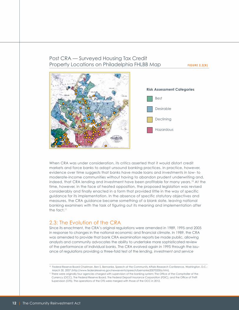
By enacting the CRA, Congress sought to halt the practice of systematically denying credit to residents and businesses in low-income neighborhoods, a practice that has come to be known as redlining. Ironically, the term redlining has its origins in a program adopted by the federal government. In 1934, the Federal Home Loan Bank Board (FHLBB) commissioned maps to be drafted for the nation’s 234 largest cities. The maps were intended to identify those areas determined to be the most and least risky neighborhoods in which to make mortgage loans. The areas demarcated with red lines were considered the most risky areas in which to make loans and were even categorized as “hazardous.” Figure 2.2(A) displays the FHLBB map of Philadelphia.
Since 1934, when the maps were commissioned, clearly much has changed in Philadelphia. Using the criteria established by the FHLBB, areas once described as “best” neighborhoods might be described by the mapmakers as “hazardous” today and vice versa. However, Philadelphia’s south side was home to many low-income neighborhoods in 1934, and that continues to be the case today. Nonetheless, one change that has taken place is the development of numerous low-income housing tax credit projects, principally made by CRA-driven bank investors in many of the formerly redlined “hazardous” neighborhoods. Figure 2.2(B) shows the same FHLBB map of Philadelphia, with housing tax credit properties reported by survey respondents plotted.
Philadelphia Federal Home Loan Bank Board Map—19349 FiguRe 2.2(A)
Risk Assessment Categories
Best
Desirable
Declining
Hazardous
9 National Archives. Home Owners Loan Corporation Map from the Federal Home Loan Bank Board; http://www.archives.gov/index.html.
| The Community Reinvestment Act12
10 Federal Reserve Board Chariman, Ben S. Bernanke, Speech at the Community Affairs Research Conference, Washington, D.C.; March 30, 2007 (http://www.federalreserve.gov/newsevents/speech/bernanke20070330a.htm).
11 There were originally four agencies charged with supervision of the banking system: The Office of the Comptroller of the Currency (OCC), The Federal Reserve Board, The Federal Deposit Insurance Corporation (FDIC), and the Office of Thrift Supervision (OTS). The operations of the OTS were merged with those of the OCC in 2012.
When CRA was under consideration, its critics asserted that it would distort credit markets and force banks to adopt unsound banking practices. In practice, however, evidence over time suggests that banks have made loans and investments in low- to moderate-income communities without having to abandon prudent underwriting and, indeed, that CRA lending and investment have been profitable for many years.10 At the time, however, in the face of heated opposition, the proposed legislation was revised considerably and finally enacted in a form that provided little in the way of specific guidance for its implementation. In the absence of specific statutory objectives and measures, the CRA guidance became something of a blank slate, leaving national banking examiners with the task of figuring out its meaning and implementation after the fact.11
2.3: The Evolution of the CRASince its enactment, the CRA’s original regulations were amended in 1989, 1995 and 2005 in response to changes in the national economic and financial climate. In 1989, the CRA was amended to provide that bank CRA examination reports be made public, allowing analysts and community advocates the ability to undertake more sophisticated review of the performance of individual banks. The CRA evolved again in 1995 through the issu-ance of regulations providing a three-fold test of the lending, investment and service
Post CRA — Surveyed Housing Tax Credit Property Locations on Philadelphia FHLBB Map FiguRe 2.2(B)
Risk Assessment Categories
Best
Desirable
Declining
Hazardous

A CohnReznick Report | 13
activities of banking institutions within their assessment areas.12 In subsequent years, the examining agencies focused more on assessing the effectiveness of the CRA, and in 2005 expanded the definition of “community development” to include lending, investment and services to middle-income communities in distressed rural areas and in Federal Emergency Management Agency (FEMA) designated disaster areas.
The regulations written to carry out the CRA’s intent, while extensive, are the object of regular criticism for their perceived lack of clarity. One of the areas that has proven chal-lenging to interpret and administer is the meaning of the term “assessment area.”
The CRA does not actually make reference to the term assessment area. The statute provides that regulated financial institutions must “…demonstrate that [their] deposit facilities serve the convenience and the needs of the communities in which [they] are chartered to do business.”13 The statute also directs supervisory agencies to assess a bank’s record of meeting the credit needs of its “entire community, including low and moderate-income neighborhoods.”14
In its present form, the CRA requires that documented evaluations of a depository institu-tion’s CRA performance be made public and that the evaluation report make reference to “metropolitan area distinctions.”15 The following general principles in the regulations represent most of what the CRA tells us about geography:
• A bank’s CRA performance should be evaluated in those communities in which it collects deposits.
• The primary geographical measuring point is the Metropolitan Statistical Area (MSA).
• The appropriate assessment area for banks conducting business in multiple states will be determined by either the bank’s regulator or by the bank in consultation with its regulator.
In writing the regulations regarding assessment areas, the supervisory agencies were conscious that delineating specific boundaries might be problematic and give rise to assess-ment areas that were too large, too small or that did not reflect the political jurisdictions within which a bank principally was conducting business. As a result, the burden of delineating assessment areas was shifted to the banks. Banks are now obligated to define their assess-ment areas in accordance with these additional principle rules enunciated by the agencies:
• An assessment area must include one or more metropolitan statistical area.
• It may include one or more contiguous political subdivision.
• Must include the “geographies” (such as a census tract) in which the institution has its main office, branches, deposit-collecting ATMs and surrounding areas in which the institu-tion holds a significant number of loans.
12 Only large banks are evaluated on all three tests: lending, investment and service. Smaller banks may not be subject to the investment test. Large banks are currently defined as those having assets of $1.186 billion or more for December 31 of both of the previous two years, effective January 1, 2013. Source: http://www.ffiec.gov/cra/examinations.htm.
13 12 U.S.C. 2901, Sec. 802(a)(1)14 12 U.S.C. 2901, Sec. 804(a)(1)15 12 U.S.C. 2901, Sec. 807(b)(1) and Sec. 807(d)(2)

| The Community Reinvestment Act14
2.4: A Synergistic Relationship: The CRA and the Housing Tax Credit ProgramWhile there is no statutory linkage between the CRA and the housing tax credit program, the Act and the program have evolved in ways that have made them inextricably linked. As noted, CRA compliance has become the single biggest driver of the equity market for housing credit investments for over a decade. While a number of CRA-qualified investment options exist, most banks identify housing credit investments as a preferred option among the various alternatives. The reasons for this include:
• Committing equity to a housing tax credit property means that the investment will auto-matically be treated as a qualified community development investment under the CRA’s investment test requirements.
• Housing tax credit properties are rarely foreclosed upon, which has provided investors a high degree of confidence that they will receive both the return of their capital and the projected yield on their capital over the life of the investment. Other forms of CRA investment, by contrast, may offer marginal financial benefits and/or a less attractive risk/reward profile.
• Most housing tax credit investments are structured by syndication firms that in turn bear the majority of the responsibility for acquisition due diligence and for ongoing asset management. As a result, housing tax credit investments do not require the same alloca-tion of internal bank resources than may be the case for investments that banks originate and manage directly.
• An investment in a housing tax credit “fund” offers both risk diversification and yields that are generally well in excess of the bank’s cost of capital.
For 18 of the past 20 years, demand for housing tax credit investments has risen steadily while the volume of available housing tax credits, subject to a fixed limit under the autho-rizing statute, has grown at a much slower pace. The sole exception to this trend occurred in 2008 and 2009, when the equity market for housing credits was affected by the depar-ture of its two largest investors, Fannie Mae and Freddie Mac, coupled with sharply lower demand from financial services companies. Notwithstanding the reduction in demand for housing credit investments during this period, CohnReznick estimates that the total market share of CRA-motivated bank investors actually increased to nearly 100% in 2009, the year in which the equity market reached its recent low point ($4.5 billion in total equity in 2009 vs. $9 billion in 2006). Given the fact that nearly every national bank suffered financial losses in 2008 and 2009, the increase in the banking sector’s market share during this period can only be understood by the power of CRA as an investment objective. Three years after the sharp dip in the equity market, two of the largest U.S. banks, despite having no current need for housing tax credits, and billions of dollars in suspended tax benefits, continue to be major housing tax credit investors. For these banks, the apparent motivation for their continued housing tax credit investment is maintenance of their outstanding CRA ratings under the Act’s investment test.

A CohnReznick Report | 15
In recent years, the demand for housing tax credit investment among the largest national banks has expanded significantly as the banks have grown through mergers and acquisi-tions, as well as through the consolidation of the banks that failed between 2008 and 2010. As the largest banks have expanded, their CRA assessment areas have grown rapidly and now overlap each other in an increasing number of markets, primarily in urban centers along the coasts and in the most densely populated cities. The impact of this consolidation has been profound. Accordingly, the Federal Reserve Bank in Dallas reported that since 1970, the share of assets controlled by the five largest banking institutions in the U.S. has tripled from 17% to 52%.16
1970■ Top 5 Banks . . . . . . . . . . . . . . . . . 17%
■ Large and Medium Banks (95) . . . . . . . . . . . . . . . . . . 37%
■ Smaller Banks (12,500) . . . . . . 46%
2010■ Top 5 Banks . . . . . . . . . . . . . . . . . 52%
■ Large and Medium Banks (95) . . . . . . . . . . . . . . . . . . 32%
■ Smaller Banks (5,700) . . . . . . . 16%
46%
32%
37%
52%
17%
16%
Asset Concentrations Among U.S. Banks FiguRe 2.4.1
As the top five banks’ share of the total deposit base has grown, so too has their CRA investment volume. CohnReznick estimates that the top five U.S. banks now control roughly 50% of the housing tax credit equity market.
16 Source: Federal Reserve Bank of Dallas. “2011 Annual Report.”
| The Community Reinvestment Act16
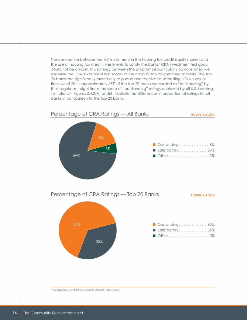
The connection between banks’ investment in the housing tax credit equity market and the use of housing tax credit investments to satisfy the banks’ CRA investment test goals could not be clearer. This synergy between the programs is particularly obvious when we examine the CRA investment test scores of the nation’s top 20 commercial banks. The top 20 banks are significantly more likely to pursue and receive “outstanding” CRA evalua-tions. As of 2011, approximately 65% of the top 20 banks were rated as “outstanding” by their regulator—eight times the share of “outstanding” ratings achieved by all U.S. banking institutions.17 Figures 2.4.2(A) and(B) illustrate the differences in proportion of ratings for all banks in comparison to the top 20 banks.
■ Oustanding . . . . . . . . . . . . . . . . . . 8%
■ Satisfactory . . . . . . . . . . . . . . . . . 89%
■ Other . . . . . . . . . . . . . . . . . . . . . . . . 3%89%
3%
8%
Percentage of CRA Ratings — All Banks FiguRe 2.4.2(A)
■ Oustanding . . . . . . . . . . . . . . . . . 65%
■ Satisfactory . . . . . . . . . . . . . . . . . 35%
■ Other . . . . . . . . . . . . . . . . . . . . . . . . 0%
65%
35%
Percentage of CRA Ratings — Top 20 Banks FiguRe 2.4.2(B)
17 Interagency CRA Rating Search Module; FFIEC.com.

A CohnReznick Report | 17
The dramatic difference in the distribution of outstanding ratings between the top 20 banks and the rest of the banking sector is a direct consequence of the differences in banks’ motivations:
• Every bank that enjoys the benefit of Federal Deposit Insurance must agree to comply with the requirements of the CRA.
• Every holding company must have at least a “satisfactory” rating before it can apply to change its charter, open a branch, expand into a new business or merge with or acquire another bank.
• Large banks view securing and maintaining an outstanding CRA rating as a way to compete with their peers and to optimize their prospects for regulatory approval of acquisitions, changes in their charter, etc.
2.5: The Geographical MismatchClearly, the largest banks have the greatest incentive to pursue outstanding CRA ratings. Since CRA performance evaluation is principally driven based upon where deposits are located, the largest, most densely populated cities and money centers attract the largest dollar volume of CRA commitments with respect to satisfying the Act’s lending and invest-ment tests. This is compounded by the fact that the current evaluation methodology does not adjust the deposit volume in money centers to net out deposits held for individuals and corporations that are physically located in other areas, or for foreign deposits. Thus, if a large Omaha-based investment firm transfers its free cash to a New York-based bank, the New York bank’s, as opposed to the Omaha bank’s, expected level of performance with respect to CRA lending and investment in the New York metropolitan area will increase.18 For that reason, the headquarters of a national bank will generate a disproportionately large amount of the bank’s core capital and, with that, a disproportionately large compo-nent of the bank’s CRA obligation. These factors have the effect of funneling CRA capital to the cities with the largest deposit base.
By contrast, housing tax credits are allocated in a manner that reflects local housing priori-ties rather than population, deposit volume or similar quantitative methodology. Under IRC Section 42, the distribution of housing tax credits is delegated to states, which in turn desig-nate a state housing credit agency to decide the manner in which the share of housing tax credits will be allocated.19 States are required to produce annual qualified allocation plans that are intended to reflect the state’s most pressing housing needs. The process by which housing priorities are determined typically ensures that housing tax credits will be awarded to projects in as many areas of the state as possible. For this reason, a dispropor-tionately smaller amount of housing credits will typically be awarded to center cities when viewed strictly from a population perspective.
18 We looked at bank deposit volume in Chicago to test this issue, and found that total deposits in Cook County were three times the average volume of total deposits in suburban counties, on a per capita basis, even though Cook County area median income is significantly lower.
19 A handful of states have designated more than one agency for this purpose.

| The Community Reinvestment Act18
From a geographical perspective, the CRA and the housing tax credit program operate according to such different distribution methodologies that they are virtually guaranteed to conflict with one another. This is exacerbated by the fact that housing tax credits are such a scarce commodity. The amount of housing tax credits allocated to a given state cannot begin to scratch the surface of the need for affordable housing in that state.20 The state allocating agencies that award credits to specific projects are mindful of the fact that low-income seniors and families need affordable housing in every congressional district in their state. The agencies’ housing priorities are based on a multitude of factors such as serving tenants with special needs, access to tenant services, the quality of the project’s sponsorship, demand for three- or four-bedroom units in some areas versus one-bedroom units in others and how tenant incomes compare with the income levels and rents of other tenants and properties in the market.
Ultimately, the manner in which CRA assessment areas are defined and investment test objectives are measured is a function of where the highest levels of bank activity occur. Housing credits are allocated, by contrast, by who the tenants are and how their needs can be met. While housing credit allocations are by no means blind to population, they are also clearly not driven by it.
The divergence between the manner in which the CRA directs investment capital and where housing credit projects are located tends to heighten what is already a mismatch between demand and supply. For many years, housing tax credit analysts have pointed to the difference in how housing tax credits are priced as being the direct consequence of that imbalance. Other observers have taken the view that if housing tax credits are more expensive in certain markets, it is simply a reflection of the lower level of real estate risk and/or higher real estate values in those markets.
CohnReznick undertook an analysis of whether and to what extent tax credits trade at different prices based on location. We then matched geographies with high and low CRA value to determine whether these locations matched up with any such differences with “CRA-hot” areas having high CRA value and “CRA-not” areas having limited CRA value. While most syndicators and investors accept the premise that housing credits are more expensive in some markets, there is less than universal agreement on the cause of such differences and whether any impact that the CRA may have on pricing is a positive or negative outcome. Before CohnReznick undertook this study, the only published objective analysis that we are aware of concerning this issue was recently undertaken by the U.S. Government Accountability Office (GAO). The GAO’s report on this issue, titled Community Reinvestment Act: Challenges in Quantifying its Effect on Low-Income Housing Tax Credit Investment, found that tax credit pricing does vary by area and that the differences in housing tax credit pricing were substantial in certain markets. Their report concludes that: (i) measuring the impact of CRA on pricing is very complex; (ii) there were several possible causes for differential pricing; and (iii) the GAO could not conclude based on its data that the CRA was the principal cause of differential pricing.
20 According to the Joint Center for Housing studies of Harvard University’s report, “The State of the Nation’s Housing 2012,” 20.2 million of U.S. households were severely rent burdened in 2010, i.e., having to contribute more than 50% of household income to rent.

A CohnReznick Report | 19
ChApteR 3:
Study Methodology
CohnReznick has undertaken an analysis of the degree to which CRA investment test compliance impacts the cost of housing tax credit
equity based on the following methodology. We began with the premise that CRA assessment areas are not exclusive to any one bank, that they overlap in many metropolitan areas and that the number of overlapping assessment areas and the concentration of deposits within them ultimately drives whether a market will be CRA-hot or CRA-not. Rather than rely on data from the state allocating agencies, CohnReznick focused on leveraging the database compiled to study the operating performance of housing tax credit properties.21
As previously noted, the assessment area rules are unfortu-nately complex. The demarcation of an assessment area includes those areas in which the bank has its headquarters branch, its satellite branches and deposit-collecting ATMs, as well as surrounding areas in which the bank has originated or purchased a majority of its loans. For multistate banks, the regulators evaluate CRA performance in every multi-state metropolitan area and for each state within that area. These “subratings” are then weighted by deposit volume to produce the bank’s overall CRA rating.22 As noted above, this evaluation methodology funnels CRA capital into large,
densely populated cities with a disproportionate percentage of the bank’s overall deposit base. This is of course particularly true of the nation’s largest banks.
Given the phenomenon of capital concentration in the banking system, CohnReznick focused on the CRA assessment area profiles of the 20 largest US commercial banks. This subset of banks represents a high percentage of the housing credit equity market and a correspondingly high percentage of all U.S. bank deposits. By focusing on commercial banks, CohnReznick deliberately excluded certain large banks that have limited CRA obligations by reason of their focus on nontraditional banking services. Figure 3.1 illustrates the list of banks selected for this analysis as well as the name of each bank’s regulator, the size of its asset base and its most recent CRA rating. While seven of these banks received “satisfactory” overall evaluations, all 20 received “outstanding” investment test evaluations in most of their individual assessment areas.
21 “The Low-Income Housing Tax Credit Program at year 25: An Expanded Look at Its Performance.” A list of data providers is included as Appendix A.
22 The largest national banks can have 500 or more individual assessment areas in which they have CRA obligations.

| The Community Reinvestment Act20
RANk* iNStitutioN NAme heADquARteRS totAl ASSetS** RegulAtoR lAteSt CRA SCoRe***
1 JP Morgan Chase New York, NY $2,359,141,000 OCC Outstanding
2 Bank of America Charlotte, NC $2,212,004,452 OCC Outstanding
3 Citigroup, Inc. New York, NY $1,864,660,000 OCC Outstanding
4 Wells Fargo San Francisco, CA $1,422,968,000 OCC Outstanding
5 U.S. Bancorp Minneapolis, MN $353,855,000 OCC Outstanding
6 PNC Financial Services Pittsburgh, PA $305,285,879 OCC Outstanding
7 Capital One Mclean, VA $206,103,658 FRB Outstanding
8 TD Bank US Portland, ME $218,916,640 OCC Outstanding
9 BB&T Corp Winston-Salem, NC $183,872,371 OTS Satisfactory
10 Suntrust Banks Atlanta, GA $173,566,088 FRB Satisfactory
11 RBS Citizens
Financial Group
Providence, RI $127,911,732 OCC Outstanding
12 Regions Financial Birmingham, AL $121,347,388 FRB Satisfactory
13 Fifth Third Bank Cincinnati, OH $121,893,748 FRB Satisfactory
14 BMO Financial Corp Wilmington, DE $116,109,476 OCC Satisfactory
15 Union Bank San Francisco, CA $96,992,464 OCC Outstanding
16 KeyCorp Cleveland, OH $89,425,613 OCC Outstanding
17 M&T Bank Corporation Buffalo, NY $83,008,803 FRB Outstanding
18 Bancwest Honolulu, HI $79,869,488 FDIC Satisfactory
19 Comerica Bank Dallas, TX $65,398,175 FRB Outstanding
20 Huntington Bank Columbus, OH $56,153,185 OCC Satisfactory
Top 20 U.S.-based Commercial Banks FiguRe 3.1
* Ranked in the order of total assets as of December 31, 2012. Banks that are considered not subject to CRA mandate have been excluded from this list. ** Total assets were as of December 31, 2012 (displayed in thousand dollars) and taken from http://www.ffiec.gov/nicpubweb/nicweb/Top50Form.aspx. *** The four banking regulators assign an overall CRA rating using a four-tiered rating system: Outstanding, Satisfactory, Needs to Improve, and Substantial Noncompliance.

A CohnReznick Report | 21
Given the very large number of assessment areas for these banks, CohnReznick initially hoped to use the public CRA reports submitted to the Federal Financial Institutions Examination Council and aggregate those data to an organization level in order to assemble a comprehensive list. The public investment test reporting is compiled in an exhaustive series of PDFs that did not permit easy construction of a database. After consultation with one of the CRA regulatory agencies, it was agreed that the location of individual bank branches was a reasonable proxy for the geographic areas that govern the assessment areas for these banks.
We utilized the Federal Deposit Insurance Corporation’s website to obtain the address of every branch location for the top 20 commercial banks. The bank branch location data were exported into spreadsheet format for sorting and editing. Once foreign branches were removed from the dataset, address information for 35,479 bank branch locations in 10,697 zip codes (this represents approximately 25% of the zip codes in the United States) remained. This data were uploaded into Maptitude, mapping software published by the Caliper Corporation, a firm that specializes in geographic information software.

| The Community Reinvestment Act22
The bank branch locations were plotted by address on a U.S. map using their five-digit zip codes. Based on the number of bank branches located in each zip code, CohnReznick color coded the boundaries of each zip code to identify the CRA value of an investment
in that area. For this purpose we established five levels of bank branch concentration and characterized these as “heat zones.” Areas with the highest branch concentration are referred to as Zone 5. Due to the absence of academic research around the effect of investment test concentra-tion, we were left to devise our own for measuring investment concentration.23 Therefore, CohnReznick stratified the zones. The color orange denotes Zone 5, which we define as an area with more than 10 bank branches maintained by the nation’s top 20 U.S. banks and thus an area we deemed to have the highest level of CRA value for investment test purposes. The
question of whether there should be more or fewer zones to test for concentration and whether the number of bank branches is the most appropriate metric, we leave to those who may pursue this initiative in the future.
The use of five zones is arguably a more conservative approach than needed. The fact that the methodology was utilized uniformly across every market is a further demonstra-tion of our interest in supporting a conclusion rather than a predetermined premise. Given the fact that the same bank can have multiple branches within a single zip code, we found that in a small handful of zip codes, there were more than 20 individual branches operated by the top banks. Not surprisingly most of these “very” CRA-hot areas are located in zip codes 10019–10022, which correspond to Manhattan, New York and the surrounding boroughs.
CRA heAt ZoNe DeSigNAtioN NumBeR oF top 20 uS BANk BRANCheS
Zone 1 0 branches
Zone 2 1-2 branches
Zone 3 3-5 branches
Zone 4 6-9 branches
Zone 5 10 or more branches
Heat Map Key FiguRe 3.2
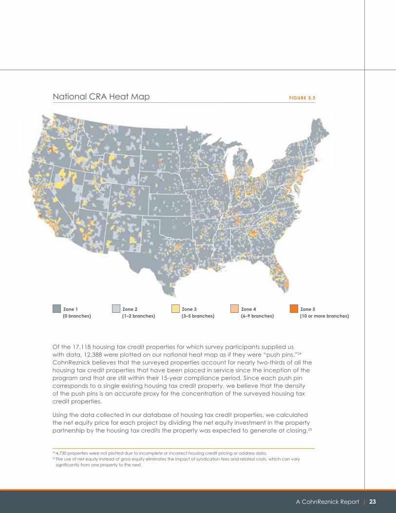
The composite effect of identifying all of the zip codes in the country with bank branch concentration provided us with what we have referred to here as a National CRA Heat Map. The map is illustrated in Figure 3.3.
23 By contrast, a great deal of research has been conducted with respect to measuring the CRA’s impact on mortgage lending.
A CohnReznick Report | 23
Of the 17,118 housing tax credit properties for which survey participants supplied us with data, 12,388 were plotted on our national heat map as if they were “push pins.”24 CohnReznick believes that the surveyed properties account for nearly two-thirds of all the housing tax credit properties that have been placed in service since the inception of the program and that are still within their 15-year compliance period. Since each push pin corresponds to a single existing housing tax credit property, we believe that the density of the push pins is an accurate proxy for the concentration of the surveyed housing tax credit properties.
Using the data collected in our database of housing tax credit properties, we calculated the net equity price for each project by dividing the net equity investment in the property partnership by the housing tax credits the property was expected to generate at closing.25
24 4,730 properties were not plotted due to incomplete or incorrect housing credit pricing or address data.25 The use of net equity instead of gross equity eliminates the impact of syndication fees and related costs, which can vary
significantly from one property to the next.
National CRA Heat Map FiguRe 3.3
Zone 1 Zone 2 Zone 3 Zone 4 Zone 5 (0 branches) (1–2 branches) (3–5 branches) (6–9 branches) (10 or more branches)

| The Community Reinvestment Act24
This analysis provided 16,953 valid results, which we further filtered by excluding data from projects considered to be outliers. Approximately 25% of the surveyed properties were excluded from this study because the pricing data reported for those projects represented a material variance from our median pricing data.26 For example, we requested that survey participants exclude equity related to the acquisition of state tax credits (which trade at substantially lower prices) and historic tax credits (which can also trade at very different levels). Upon review of the data, however, it was apparent that several respondents failed to follow our request to net out the state credit and/or historic credit equity component. After screening out these additional outlier projects, 12,388 properties remained.
Several caveats are appropriate regarding the subject of tax credit “pricing.” In the first instance, housing tax credits cannot be traded for cash. In order for an investor to be allocated housing tax credits, it must become an owner in the partnership that owns the property. Thus the phrase “tax credit pricing” is simply shorthand for the ratio of an investor’s long-term equity commitment to a given property and the housing tax credits it expects to claim. We use the terms “tax credit pricing” and “net equity pricing” inter-changeably in this report.
We appreciate the fact that the use of the tax credit price as a simplifying assumption can be misleading. Thus, for example, assume that there are two housing tax credit invest-ments with the same pricing profile—$8.5 million of equity for $10 million of credits. In the first case, an investor might be required to contribute 100% of the equity requirement at closing. If the equity investment had been spread over a three-year period, the nominal tax credit price would be the same, but the two investments would produce very different rates of return. In the same way, a housing credit project financed with tax-exempt bonds
26 In general, we classified properties as outliers when the tax credit price was less than $0.60 and greater than $1.35.

A CohnReznick Report | 25
will typically generate higher tax losses because of higher interest expense deductions. Having acknowledged these variations, there is no data to suggest that properties located in CRA-hot areas are more likely to have multiyear pay-in schedules than properties in CRA-not locations. Thus, while the use of tax credit pricing is not a perfect proxy for cost, variations of this type are unlikely to have a meaningful impact on the outcome in the context of a dataset this large.
In addition to calculating the tax credit price for each project, we tracked the year in which the property was placed in service or was expected to be placed in service. Given that the development timeline for a typical housing credit project is one-two years, the year a project is placed in service reflects a one- to two- year delay from the date in which the equity price was determined.27 We adopted a unifying assumption that the net equity price was determined two years before the project was actually placed in service.
Finally, because it is common for housing tax credit projects to experience delays in construction or lease-up, developers are typically required to make so-called adjuster payments to equity investors to make them whole from a yield perspective. We asked respondents to provide us with the originally agreed-upon net equity investment and projected credits at closing to ensure that net equity assumptions would be compared on a consistent basis.
Notwithstanding the efforts made to conduct our analysis thoughtfully, there are limita-tions to our findings, largely because of the complexity of this undertaking, and adopting assumptions that must be simplified to arrive at a conclusion. Thus, for example, while we identified bank branch locations for the top 20 banks, we did not include data to weight each location by the volume of deposits maintained in each branch. Had we done so, the designation of CRA-hot zones would presumably have reflected sharper distinctions between the hottest and coldest markets in instances where the number of bank branches may not have been a good indicator of deposit volume.
Once the processes of plotting the surveyed properties, calculating their tax credit prices and screening for bad data were complete, we began to study the data on a national, state and metropolitan-area basis to look for evidence of differential tax credit pricing in CRA-hot versus CRA-not locations.
27 There are cases where the timing gap between the date the tax credit price was determined and when the underlying property was placed in service has been significantly longer than anticipated.

| The Community Reinvestment Act26
4.1: CRA Impact on the Availability of Housing Tax Credit Equity
As previously stated, there is a clear and unassailable relationship between the CRA investment test value of a housing tax credit invest-
ment and its geographic location. This outcome is essentially guaranteed by the concentration of bank deposits in the hands of the largest national banks, which in turn conduct a disproportionate amount of their business in urban centers. The fact that a large portion of the available housing tax credits are being acquired by the same top five banks that control 52% of all U.S. bank deposits is unlikely to be a coincidence.
The properties CohnReznick surveyed are located in 7,438 zip codes in all 50 states in markets that range from CRA-hot to CRA-not. As Figure 4.1.1 illustrates, every housing credit property is represented by a single push pin. The density of those push pins corresponds to the concentration of housing credit capital.
ChApteR 4:
Findings: The Impact of the CRA on the Housing Tax Credit Program
Surveyed Properties on CRA Heat Map FiguRe 4.1.1
Zone 1 Zone 2 Zone 3 Zone 4 Zone 5 (0 branches) (1–2 branches) (3–5 branches) (6–9 branches) (10 or more branches)
A CohnReznick Report | 27
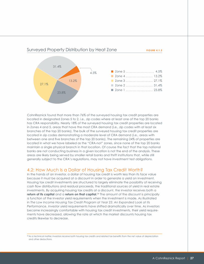
■ Zone 5 . . . . . . . . . . . . . . . . . . . . . 4.5%
■ Zone 4 . . . . . . . . . . . . . . . . . . . . 13.2%
■ Zone 3 . . . . . . . . . . . . . . . . . . . . 27.1%
■ Zone 2 . . . . . . . . . . . . . . . . . . . . 31.4%
■ Zone 1 . . . . . . . . . . . . . . . . . . . . 23.8%
4.5%
27.1%
31.4%
13.2%
23.8%
Surveyed Property Distribution by Heat Zone FiguRe 4.1.2
CohnReznick found that more than 76% of the surveyed housing tax credit properties are located in designated Zones 5 to 2, i.e., zip codes where at least one of the top 20 banks has CRA responsibility. Nearly 18% of the surveyed housing tax credit properties are located in Zones 4 and 5, areas that have the most CRA demand (i.e., zip codes with at least six branches of the top 20 banks). The bulk of the surveyed housing tax credit properties are located in zip codes demonstrating a moderate level of CRA demand (i.e., areas with between one and five branches of the top 20 banks). The remaining 24% of properties are located in what we have labeled as the “CRA-not” zones, since none of the top 20 banks maintain a single physical branch in that location. Of course the fact that the top national banks are not conducting business in a given location is not the end of the analysis. These areas are likely being served by smaller retail banks and thrift institutions that, while still generally subject to the CRA’s regulations, may not have investment test obligations.
4.2: How Much Is a Dollar of Housing Tax Credit Worth? In the hands of an investor, a dollar of housing tax credit is worth less than its face value because it must be acquired at a discount in order to generate a yield on investment. Housing tax credit investments are structured to largely eliminate the possibility of receiving cash flow distributions and residual proceeds, the traditional sources of yield in real estate investments. By acquiring housing tax credits at a discount, the investor receives both a return of its capital and a return on that capital.28 The amount of the discount is principally a function of the investor yield requirements when the investment is made. As illustrated in The Low Income Housing Tax Credit Program at Year 25: An Expanded Look at Its Performance, investor yield requirements have shifted dramatically over time. As investors became increasingly comfortable with housing tax credit investments, their yield require-ments have decreased, allowing the rate at which the market discounts housing tax credits likewise to decrease.
28 As a technical matter, investors receive both housing tax credits and related tax benefits from the net value of depreciation and other deductions.

| The Community Reinvestment Act28
When housing tax credits trade at low discount rates (i.e., high prices), the amount of equity that must be invested for each dollar of tax credit must increase. For example, when discount rates and investor yields reached historically low levels in 2006, housing tax credits were trading almost at par ($1:$1). During that year, a project with $10 million of housing credits would have attracted, on average, an equity investment of $9.5 million ($0.95/$1). If an identical project competed for capital in 2009, when weak demand forced sharply higher discount rates, an investor might have reduced its investment offer to $6.5 million ($0.65/$1) for the same $10 million of housing credits. The loss of $3 million in capital between these hypothetical examples would require the developer to fill the financing gap by applying for a larger mortgage or by seeking additional “soft” financing from a state or local government agency.
In 2009, this meant that many housing tax credit projects that had secured development rights, received a reservation of housing tax credits and obtained an equity commit-ment from an investor or syndicator suddenly became economically infeasible. In many instances, equity commitments, most of them nonbinding, were either withdrawn or replaced with lower offers. Were it not for the passage of the Tax Credit Assistance Program and the Tax Credit Exchange Program introduced by the American Recovery and Reinvestment Act in 2009, many housing tax credit projects would have simply been impos-sible to finance.29 This is important to keep in mind because Figure 4.1.1 shows only surveyed housing tax credit properties that were completed under the housing tax credit program, and not those that opted for the Tax Credit Exchange Program in lieu of the traditional syndicated housing tax credit investment model or those that simply could not overcome the financial feasibility hurdle because of difficulty attracting tax credit equity. If an analysis of the latter were performed, we would expect to see an overwhelming portion of afford-able properties located in CRA-not markets. Anecdotal experience suggests that states with a relatively low concentration of CRA-motivated demand reported higher utilization of the Tax Credit Exchange program and a larger share of stalled projects during 2008–2009.
29 See footnote 5 for background information on the Tax Credit Assistance and Tax Credit Exchange programs.

A CohnReznick Report | 29
The housing credit market began to recover in 2010, and by the end of 2011 the demand for housing credit investments had returned to pre-2008 levels. In certain parts of the country, however, even during the bottom of the equity market, demand for housing credit investments and housing tax credit prices were impacted much less severely. The resis-tance to sharply lower tax credit prices even in the midst of a market uncertainty was most evident in the most sought after CRA markets, including cities such as New York and San Francisco, and to a much lesser extent in projects located in Indianapolis and Milwaukee.
DeCReASe iN meDiAN tAx CReDit pRiCe
2006–2008
1New York–Northern New Jersey– Long Island, NY–NJ–PA MSA
$0.10
2 San Francisco–Oakland–Fremont, CA MSA $0.11
3 Chicago–Joliet–Naperville, IL–IN–WI MSA $0.14
AveRAge $0.12
4 Cleveland–Elyria–Mentor, OH MSA $0.18
5 Milwaukee–Waukesha–West Allis, WI MSA $0.19
6 Indianapolis–Carmel, IN MSA $0.22
AveRAge $0.20
Housing Tax Credit Pricing Trend for Selected MSAs (2006–2008) FiguRe 4.2.1
Given the sharp decline in equity demand during 2008, tax credit prices should have moved sharply lower, and as Figure 4.2.2 illustrates, that is exactly what happened in most of the country. While virtually all markets witnessed a downward trend in pricing from 2006 to 2008, the pricing reduction in the three CRA-hot MSAs averaged $0.12 per dollar of credit versus $0.20 per dollar of credit in the three CRA-not MSAs. The only way that we believe the resistance to sharply lower pricing can be explained is to credit the powerful influence that the CRA has on these CRA-hot markets.
Figure 4.2.2 illustrates the 2008 median housing tax credit pricing for selected MSAs. As previously noted, 2008 represents the bottom of the tax credit market over the past 15 years. CohnReznick has chosen a sampling of MSAs to illustrate the spread in median pricing from top to bottom.

| The Community Reinvestment Act30
meDiAN houSiNg tAx CReDit pRiCe30
populAtioN RANk
DepoSit peR CApitA RANk
San Francisco–Oakland–Fremont, CA MSA
$1.06 12 1
Los Angeles–Long Beach–Santa Ana, CA MSA
$1.00 2 17
New Orleans–Metairie–Kenner, LA MSA
$0.99 N/R N/R
Washington–Arlington–Alexandria, DC–VA–MD–WV MSA
$0.98 7 10
Seattle–Tacoma–Bellevue, WA MSA $0.98 15 25
New York–Northern New Jersey– Long Island, NY–NJ–PA MSA
$0.95 1 4
Miami–Fort Lauderdale–Pompano Beach, FL MSA
$0.93 8 13
Philadelphia–Camden–Wilmington, PA–NJ–DE–MD MSA
$0.90 6 2
Des Moines–West Des Moines, IA MSA $0.74 N/R N/R
Milwaukee–Waukesha–West Allis, WI MSA
$0.70 N/R N/R
Grand Rapids–Wyoming, MI MSA $0.69 N/R N/R
Indianapolis–Carmel, IN MSA $0.68 35 29
2008 Median Housing Tax Credit Pricing for Selected MSAs FiguRe 4.2.2
30 Population and population by MSA data obtained from the United States Census Bureau; http://www.census.gov/population/metro/.
A CohnReznick Report | 31
Demand fell sharply in 2008 following the exits of Freddie Mac and Fannie Mae from the market. The data reflected in Figure 4.2.2 are remarkable in several respects. With median pricing averaging $0.70, the downward pressure on tax credit pricing is largely attributable to decreased prices of the four MSAs shown at the bottom of the chart. While these four MSAs are all located in the Midwest, except for Indianapolis none of them make the list of the 35 largest metropolitan areas by population or per capita bank deposit volume. In contrast, the downward movement in pricing was much less pronounced in metropolitan areas with the highest population density and a disproportionate share of bank deposits. The fact that housing tax credits traded at just below $1/$1 in the most densely populated cities such as San Francisco, Los Angeles, Washington, New York and Miami, when they could have been acquired for $0.35-$0.40 less elsewhere, illustrates the power of the CRA and demonstrates the inelasticity of demand in CRA-hot markets. Note, in this context, not every city or town is located in an MSA. Roughly 16% of the U.S. residents lived outside one of the 374 MSAs in either a micro-politan area (10,000-50,000 residents) or area with fewer than 10,000 residents.31 These areas are generally Zone 1 loca-tions, and housing tax credit properties here have generated pricing below $0.70.
4.3: State-Level Tax Credit Pricing AnalysisIt has proven difficult to develop meaningful nationwide data to measure differential pricing in CRA-hot versus CRA-not markets. The reasons for this are numerous but have largely to do with the fact that the major banks have chosen self-assessment areas that do not line up neatly with metropolitan area geographies. Given the scarcity of tax credit properties in major city locations, assessment areas have apparently been expanding to include areas that are outside of city boundaries that would typically be considered suburban communities. This is particularly true, for example, in California, where the San Francisco, Los Angeles and San Diego metropolitan areas contain well over half the state’s population.32
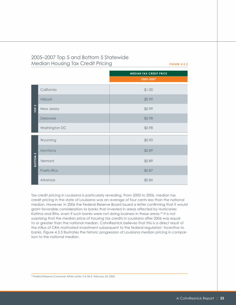
As an alternative to comparing housing tax credit prices by discrete geographies, CohnReznick analyzed the range in pricing on a state-by-state basis. As Figure 4.3.1 indi-cates, for the years 2005-2007, the median price for housing tax credits by state ranged from $1.00 in California to $0.86 for surveyed properties developed in Arkansas. For purposes of this analysis, CohnReznick chose the subset of surveyed properties that closed in 2005-2007 to minimize the impact of the 2008–2009 economic downturn.
31 Office of Management & Budget, OMB bulletin No. 10-02, December 2009.32 US Census Bureau 2011 Estimate: Los Angeles-Long Beach- Santa Ana, MSA: 12,944,804; San Francisco-Oakland-Freemont,
MSA: 4,391,037; San Diego-Carlsbad-San Marcos, MSA: 3,140,069 for a total population of 38,040,000.

| The Community Reinvestment Act32
Housing tax credit prices on a statewide basis provide useful data concerning tax credit pricing in CRA-hot vs. CRA-not markets. As Figure 4.3.2 illustrates, median housing tax credit prices are highest in states dominated by the top 20 banks and, more precisely, the top five banks in particular. It is not surprising that in Arkansas, Puerto Rico and Montana, where the number of top 20 bank branches is the lowest, tax credit prices are also the lowest. Unlike California with its major population centers, Arkansas has only one of the nation’s top 100 metropolitan areas, Little Rock, and 76% of the state’s residents live outside of this area.
ME
NY
PA
VA
NJDEMDDC
NHVTMARICT
NC
SC
GAALMS
TN
KY
OHINIL
MI
WI
MN
IA
MO
AR
TX
OK
KS
NE
SD
WY
COUT
NMAZ
NDMT
ID
NV
WA
OR
CA
LA
FL
WV
15.0% and below 15.1% to 22.0% 22.1% to 28.0% 28.1% to 34.0% 34.1% and above
2005–2007 Statewide Median Housing Tax Credit Pricing FiguRe 4.3.1
$0.90 and below $0.90 to $0.93 $0.93 to $0.95 $0.95 to $0.97 $0.97 and above
A CohnReznick Report | 33
meDiAN tAx CReDit pRiCe
2005–2007
top
5
California $1.00
Missouri $0.99
New Jersey $0.99
Delaware $0.98
Washington DC $0.98
Bo
tto
m 5
Wyoming $0.90
Montana $0.89
Vermont $0.89
Puerto Rico $0.87
Arkansas $0.86
2005–2007 Top 5 and Bottom 5 Statewide Median Housing Tax Credit Pricing FiguRe 4.3.2
Tax credit pricing in Louisiana is particularly revealing. From 2000 to 2006, median tax credit pricing in the state of Louisiana was an average of four cents less than the national median. However, in 2006 the Federal Reserve Board issued a letter confirming that it would grant favorable consideration to banks that invested in areas affected by Hurricanes Katrina and Rita, even if such banks were not doing business in these areas.33 It is not surprising that the median price of housing tax credits in Louisiana after 2006 was equal to or greater than the national median. CohnReznick believes that this is a direct result of the influx of CRA-motivated investment subsequent to the federal regulators’ incentive to banks. Figure 4.3.3 illustrates the historic progression of Louisiana median pricing in compar-ison to the national median.
33 Federal Reserve Consumer Affairs Letter, CA 06-5, February 24, 2006.

| The Community Reinvestment Act34
2006: Regulators Icentivize Investment: Louisiana vs. National Median Tax Credit Pricing FiguRe 4.3.3
meD
iAN
ho
uSi
Ng
CR
eDit
pR
iCiN
g
$1.00
$0.95
$0.90
$0.85
$0.80
$0.75
$0.702000 2001 2002 2003 2004 2005 2006 2007 2008 2009
■ Louisiana Median ■ National Median
In order to examine how differential pricing may have changed during certain time periods, we divided the 11-year period from 2000 through 2010 into three periods: 2000–2004, 2005–2007 and 2008–2010. Figure 4.3.4 is an analysis of statewide housing tax credit pricing by the three distinct time periods.
YeAR CloSeD
2000–2004 2005–2007 2008–2010
Overall Median Net Equity Price $0.88 $0.95 $0.73
Lowest Statewide Median Net Equity Price $0.77 $0.86 $0.64
Highest Statewide Median Net Equity Price $0.95 $1.00 $0.89
Price Disparity $0.18 $0.14 $0.25
Statewide Housing Tax Credit Pricing by Time Period FiguRe 4.3.4

A CohnReznick Report | 35
When the equity market was at its historical peak volume in 2006, housing tax credits were trading more or less at par, $1 for $1 in many locations. It is within this period (2005–2007) that we observed, from data collected in this study, the narrowest ($0.14) spread between states with the highest and most concentrated CRA demand and those with the least. By contrast, when economic conditions in the USA and around the world deteriorated in 2008–2009 and taxable incomes against which tax credits are applied decreased, investor demand neces-sitated significantly lower tax credit pricing. Further, given the fact that CRA-motivated banks were virtually the sole source of housing tax credit equity in the market during the 2008–2010 economic downturn, much steeper differences in price were observed between CRA-hot and CRA-not markets. During this period, a $0.24 spread was observed between some states.
4.4: Individual Market Housing Tax Credit Pricing AnalysisIn an attempt to “account” for potential differences in real estate quality, CohnReznick undertook an analysis of states with one or more large metropolitan areas to explore the pricing spread between CRA-hot and CRA-not markets in both the metropolitan areas and the state as a whole. We studied the impact of CRA on housing credit pricing in many metro-politan areas, but have chosen to present the following areas for comparative purposes:
• Indianapolis, Indiana• Little Rock, Arkansas• San Diego, California.
Without regard to the manner in which pricing is analyzed using every conceivable variable (by year, by region, by state, by property type), tax credit pricing is almost always higher in CRA heat Zones 2, 3, 4 and 5 than in Zone 1. Again, Zone 1 is where none of the top 20 U.S. commercial banks have a physical branch. In some cases, the pricing “spreads” are not as wide as might be expected. Thus, as previously suggested, tax credit pricing for housing credit properties in areas such as southern California and the greater New York metropolitan area tend to blend together as a result of “overlapping” areas of CRA investment test responsibility. In southern California, for example, we observed a grouping of projects in Zone 1 that were actually priced at higher levels than some projects in Zone 5 areas. This appears to be further evidence of the impact of increasingly wide self-assessment areas.

| The Community Reinvestment Act36
4.4.1: Indianapolis, Indiana
Indianapolis is the largest city in Indiana, and the 12th largest city in the United States, with a 2010 population of more than 825,000. Indianapolis is ranked 26th among MSAs in our dataset containing 102 properties representing 8,657 total units, 7,932 of which are low-income housing units. The surveyed housing tax credit properties represent more than $430 million of equity. The 78 stabilized properties in this dataset reported 94.0% 2010 median occupancy, which was less than the national 96.6% median. The state’s 2010 median debt coverage ratio (DCR)
and per-unit cash flow were 1.17 and $284, respectively, which were both below the national medians of 1.24 and $419.34 No
one would argue with the assertion that Indianapolis represents an urban area in Indiana with a more dense population than the rest of the state. If operating metrics and perceived real estate quality were driving credit pricing, then it would not stand to reason that proper-ties in Indiana, Indianapolis in particular, would generate median pricing consistent with the CRA-hottest areas in the country. Based on the pricing data we analyzed, it does not appear that the historical operating performance of housing tax credit properties in this market, which have lagged behind the national median, has had a meaningful impact on the price of housing credits in Indianapolis, particularly in CRA-hot areas.
meDiAN phYSiCAl oCCupANCY
meDiAN DeBt CoveRAge RAtio
meDiAN peR uNit CASh FloW
2008 2009 2010 2008 2009 2010 2008 2009 2010
National 96.4% 96.3% 96.6% 1.15 1.21 1.24 $250 $341 $419
Indiana 94.0% 94.0% 94.4% 0.85 1.05 1.14 ($228) $77 $212
Indianapolis–Carmel, IN MSA 92.6% 93.2% 94.0% 0.77 0.99 1.17 ($482) $49 $284
Operating Performance: National, Indiana and Indianapolis MSA FiguRe 4.4.1(A)
The spread in median housing tax credit pricing from the CRA-hot Zone 5 and CRA-not Zone 1 was just $0.09 for properties located throughout the State of Indiana. However, if we focus more narrowly on Indianapolis, the pricing spread more than doubled and illustrates a $0.24 difference between median housing credit pricing in zones 5 and 1.
As noted previously, both Indiana and Indianapolis properties have historically demon-strated weaker operating metrics relative to the national medians for occupancy, DCR and per-unit cash flow. The performance of properties in Indianapolis lagged behind the
34 Debt coverage ratio is defined as net operating income less required replacement reserve deposits divided by mandatory debt service payments. Per-unit cash flow is defined as available cash flow after deducting debt service payments and required replacement reserve contributions.

A CohnReznick Report | 37
state as a whole except in the year 2010. If tax credit investors were selectively investing based on the “quality” of the real estate in a given area, tax credit pricing should logi-cally have been consistently lower in Indianapolis. While at first glance this appears to be the case in desig-nated Zones 1-4, where Indianapolis properties exhibit a median price that is lower than the state median, the distribution of properties by heat zone depicts a more complete picture. For example, while surveyed Indianapolis properties located
in Zone 1 reported a median tax credit price of $0.75, which is lower than
the state median of $0.82, only 5% of surveyed Indianapolis properties are located in Zone 1. In
comparison, 18% of surveyed Indianapolis proper-ties are located in Zone 5, which bears the greatest
CRA demand from the top 20 U.S. banks. Credits for these properties were “traded” for nearly $1 for $1 of housing tax
credit. Only 9% of surveyed properties in the State of Indiana are located in Zone 5, and those reported prices that are 10 cents lower.
Indianapolis is not the only example of an MSA where properties underperform, and yet housing tax credit pricing is high in CRA-hot areas. CohnReznick observed numerous MSAs in our dataset, including Atlanta and Detroit, where we see the same phenomenon: below-median operating performance coupled with premium CRA pricing. We conclude that the CRA values of housing tax credit properties in these areas have historically over-ridden what might have otherwise been lower tax credit prices if tax credit pricing were based solely on perceived real estate quality and performance.
Zone 1
Zone 2
Zone 3
Zone 4
Zone 5
CRA Heat Map of Indiana with Surveyed Properties FiguRe 4.4.1(B)
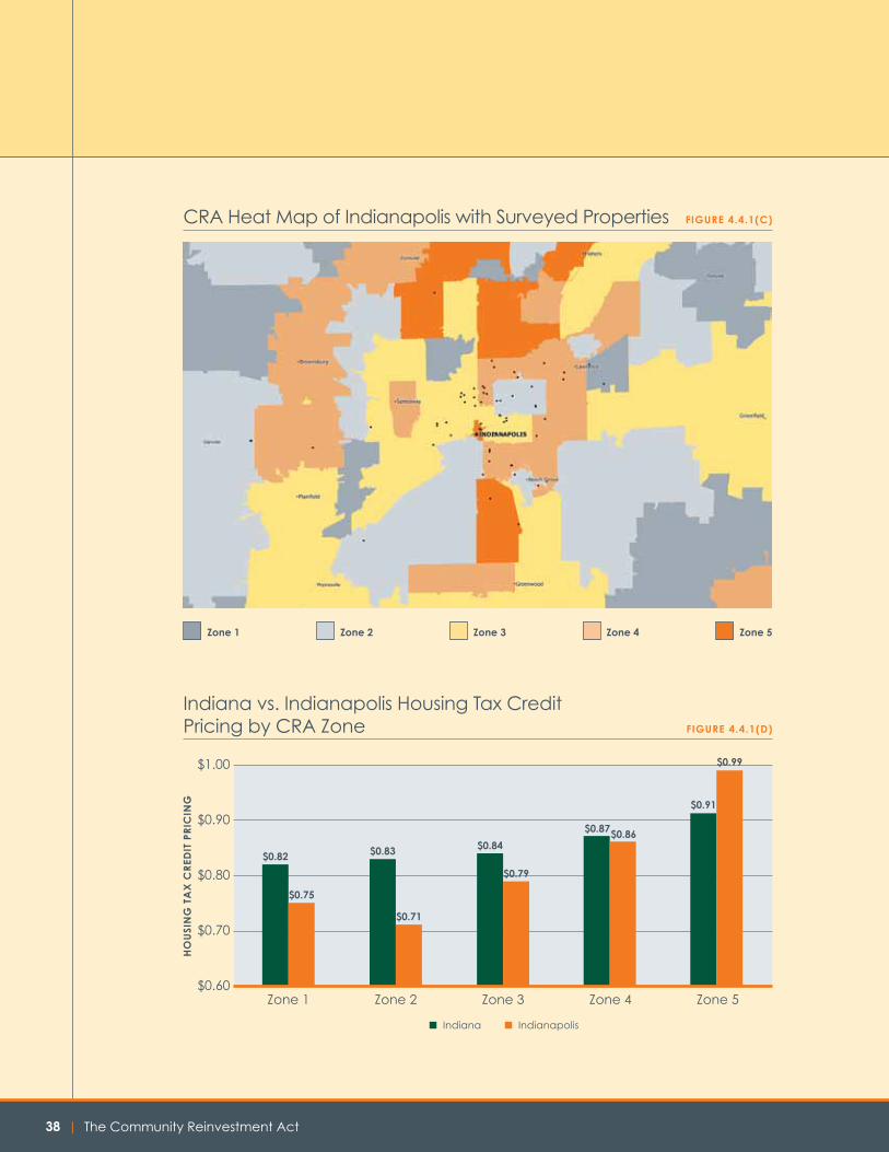
| The Community Reinvestment Act38
CRA Heat Map of Indianapolis with Surveyed Properties FiguRe 4.4.1(C)
Zone 1 Zone 2 Zone 3 Zone 4 Zone 5
Indiana vs. Indianapolis Housing Tax Credit Pricing by CRA Zone FiguRe 4.4.1(D)
Zone 1 Zone 2 Zone 3 Zone 4 Zone 5
$1.00
$0.90
$0.80
$0.70
$0.60
$0.82 $0.83 $0.84
$0.87
$0.91
ho
uSi
Ng
tA
x C
ReD
it p
RiC
iNg
$0.75
$0.71
$0.79
$0.86
$0.99
■ Indiana ■ Indianapolis

A CohnReznick Report | 39
4.4.2: Little Rock, Arkansas
Little Rock, the capital of Arkansas and its largest city, is the 47th largest city in the United States with a 2010 population of more than 193,000. Little Rock is ranked 61st among MSAs in our dataset containing 43 properties, 3,259 total units, 2,004 of which are low-income housing units. These proper-ties represent more than $95 million of equity and $101 million of housing credits. The 38 stabilized properties in this dataset reported 95.2% 2010 median occupancy, which was less than the national 96.6% median. The 2010 median DCR and per-unit cash flow were 1.02 and $7, respectively, which were both significantly less than the 1.24 and $419 national medians.
Once again, if perceived real estate quality were an overriding determinant for investment, Arkansas might not appear to be the most attractive state in which to invest. Not unlike Indianapolis, however, Little Rock reports premium housing tax credit pricing in CRA-hot areas.
meDiAN phYSiCAl oCCupANCY
meDiAN DeBt CoveRAge RAtio
meDiAN peR uNit CASh FloW
2008 2009 2010 2008 2009 2010 2008 2009 2010
National 96.4% 96.3% 96.6% 1.15 1.21 1.24 $250 $341 $419
Arkansas 96.0% 96.0% 96.0% 1.16 1.18 1.17 $179 $245 $250
Little Rock– North Little Rock–Conway, AR MSA
95.9% 95.0% 95.2% 1.04 1.08 1.02 ($47) $63 ($7)
Operating Performance: National, Arkansas and Little Rock MSA FiguRe 4.4.2(A)

| The Community Reinvestment Act40
While Arkansas had no Zone 5 areas according to CohnReznick’s criteria, its Zone 4 areas reported housing tax credit pricing that is consistent with Zone 5 areas across the country.35 The absence of Zone 5 areas is a reflection of a lower number of banks operating in Arkansas, but the pricing of the Zone 4 areas confirms that investors’ demand for CRA credit is just as strong as other CRA-hot areas of the country. The spread in median housing credit pricing from the hottest CRA Zone 4 to the CRA-not zone 1 is $0.10 in Arkansas. The pattern here is very similar to CohnReznick’s findings for Indiana. The difference in housing tax credit pricing from properties located in Little Rock in Zone 4 to those in Zone 1 was $0.20 per $1 of tax credit.
CRA Heat Map of Arkansas with Surveyed Properties FiguRe 4.4.2(B)
Zone 1
Zone 2
Zone 3
Zone 4
Zone 5
35 We note that there are very few projects located in Zone 5 areas in the State of Arkansas. In order to maintain data provider confidentiality, we have not presented the limited property pricing data we obtained for these areas.
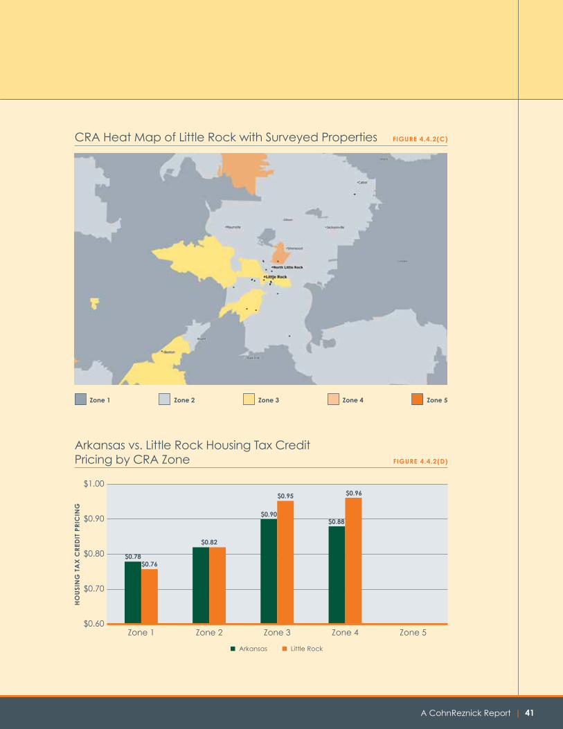
A CohnReznick Report | 41
CRA Heat Map of Little Rock with Surveyed Properties FiguRe 4.4.2(C)
Zone 1 Zone 2 Zone 3 Zone 4 Zone 5
Arkansas vs. Little Rock Housing Tax Credit Pricing by CRA Zone FiguRe 4.4.2(D)
Zone 1 Zone 2 Zone 3 Zone 4 Zone 5
$1.00
$0.90
$0.80
$0.70
$0.60
$0.78
$0.82
$0.90$0.88
ho
uSi
Ng
tA
x C
ReD
it p
RiC
iNg
■ Arkansas ■ Little Rock
$0.76
$0.95 $0.96
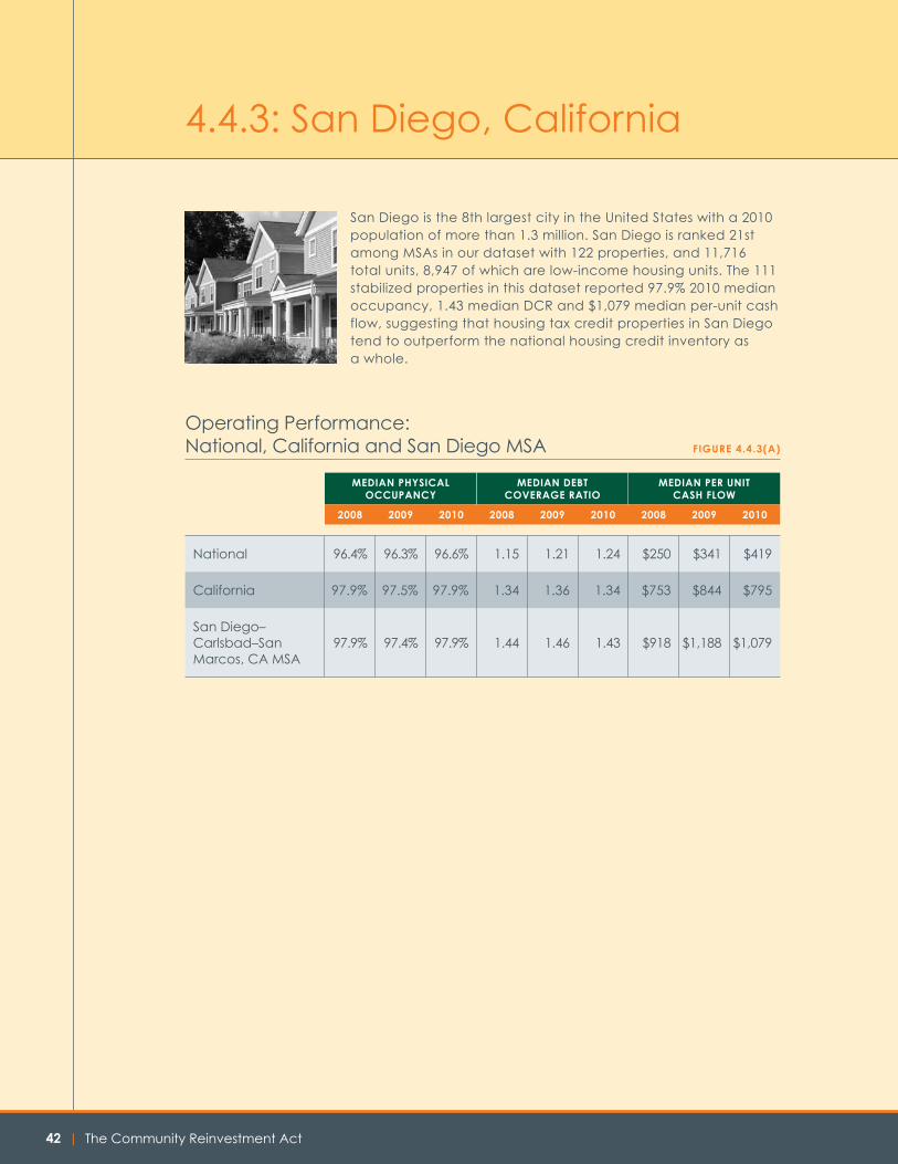
| The Community Reinvestment Act42
4.4.3: San Diego, California
San Diego is the 8th largest city in the United States with a 2010 population of more than 1.3 million. San Diego is ranked 21st among MSAs in our dataset with 122 properties, and 11,716 total units, 8,947 of which are low-income housing units. The 111 stabilized properties in this dataset reported 97.9% 2010 median occupancy, 1.43 median DCR and $1,079 median per-unit cash flow, suggesting that housing tax credit properties in San Diego tend to outperform the national housing credit inventory as a whole.
meDiAN phYSiCAl oCCupANCY
meDiAN DeBt CoveRAge RAtio
meDiAN peR uNit CASh FloW
2008 2009 2010 2008 2009 2010 2008 2009 2010
National 96.4% 96.3% 96.6% 1.15 1.21 1.24 $250 $341 $419
California 97.9% 97.5% 97.9% 1.34 1.36 1.34 $753 $844 $795
San Diego–Carlsbad–San Marcos, CA MSA
97.9% 97.4% 97.9% 1.44 1.46 1.43 $918 $1,188 $1,079
Operating Performance: National, California and San Diego MSA FiguRe 4.4.3(A)
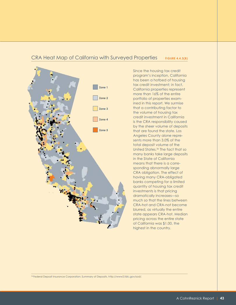
A CohnReznick Report | 43
Since the housing tax credit program’s inception, California has been a hotbed of housing tax credit investment; in fact, California properties represent more than 16% of the entire portfolio of properties exam-ined in this report. We surmise that a contributing factor to the volume of housing tax credit investment in California is the CRA responsibility caused by the sheer volume of deposits that are found the state. Los Angeles County alone repre-sents more than 3.0% of the total deposit volume of the United States.36 The fact that so many banks take large deposits in the State of California means that there is a corre-sponding abnormally large CRA obligation. The effect of having many CRA-obligated banks competing for a limited quantity of housing tax credit investments is that pricing dramatically increases—so much so that the lines between CRA-hot and CRA-not become blurred, as virtually the entire state appears CRA-hot. Median pricing across the entire state of California was $1.00, the highest in the country.
CRA Heat Map of California with Surveyed Properties FiguRe 4.4.3(B)
Zone 1
Zone 2
Zone 3
Zone 4
Zone 5
36 Federal Deposit Insurance Corporation: Summary of Deposits. http://www2.fdic.gov/sod/.
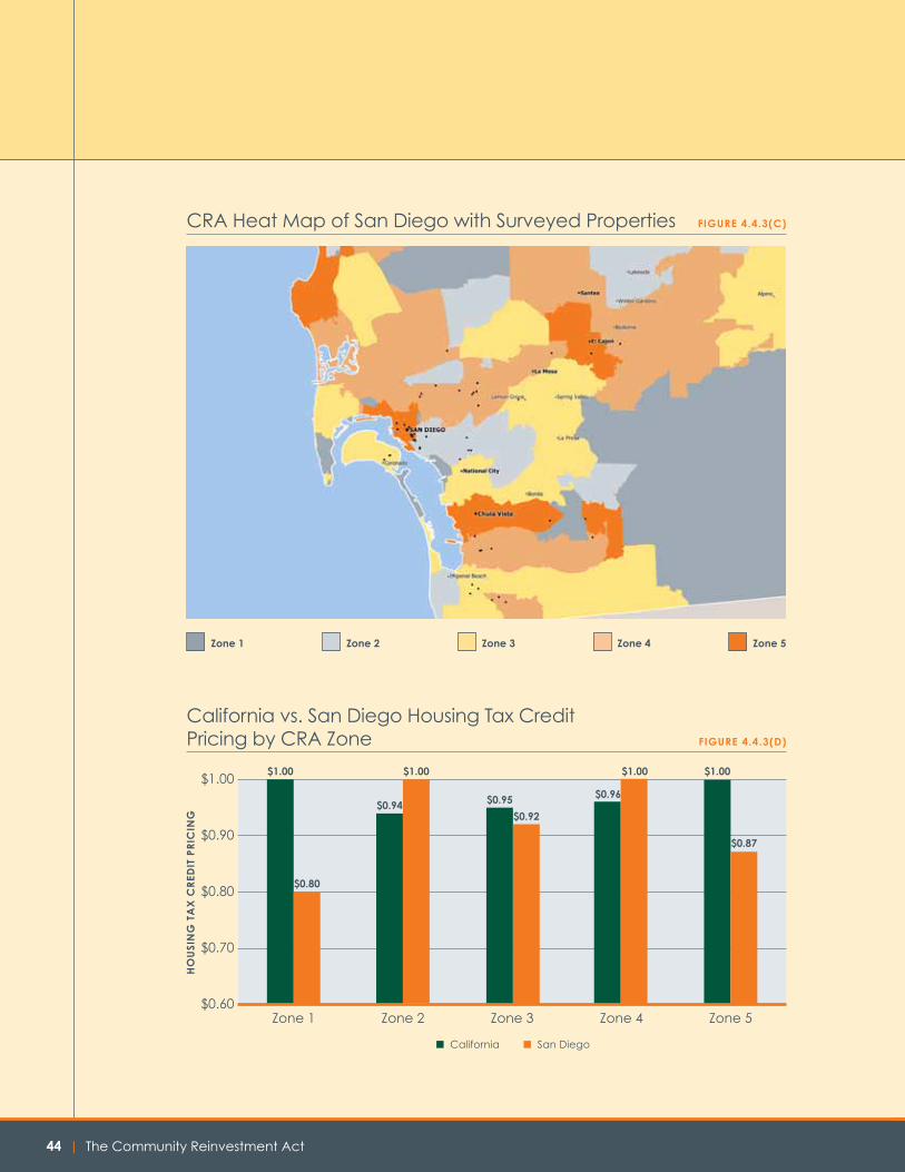
| The Community Reinvestment Act44
CRA Heat Map of San Diego with Surveyed Properties FiguRe 4.4.3(C)
Zone 1 Zone 2 Zone 3 Zone 4 Zone 5
California vs. San Diego Housing Tax Credit Pricing by CRA Zone FiguRe 4.4.3(D)
Zone 1 Zone 2 Zone 3 Zone 4 Zone 5
$1.00
$0.90
$0.80
$0.70
$0.60
$1.00
$0.94 $0.95 $0.96
$1.00
ho
uSi
Ng
tA
x C
ReD
it p
RiC
iNg
■ California ■ San Diego
$0.80
$1.00
$0.92
$1.00
$0.87
A CohnReznick Report | 45
Several trends have become apparent at this point:
• Housing tax credit pricing is almost always highest in center city locations where popula-tion density is the highest.
• While the population of Indianapolis is greater than that of San Francisco, the latter has the second highest population density in the USA, which accounts in part for the fact that housing tax credit prices are higher for projects based in San Francisco than in Indianapolis.
• The cities where CohnReznick found wider pricing spreads between CRA zones are those cities like Little Rock and Indianapolis where population density decreases dramatically once the city line is crossed.
4.5. Are There Any Factors That Drive Pricing More Than the CRA?We posit that the largest single determinant of housing tax credit pricing is based on the CRA investment test value of a given property’s location. The data CohnReznick collected clearly indicate large pricing spreads—as wide as $0.35 per $1.00 of tax credit at the extreme ends of the pricing spectrum between CRA-hot and CRA-not locations—which cannot be explained sufficiently by factors other than the CRA.
In addition to the CRA investment test value of a given property’s location, there are other factors that influence housing tax credit price:
•Overall economic and equity market condition—During 2005–2007, when the national median housing tax credit price was $0.95 and housing tax credit investment volume was at a historical high, CohnReznick observed the narrowest ($0.14 on a statewide basis) pricing spread across the country. Syndicators regularly found themselves in competition to line up projects to satisfy the demand from their investors. Even states with the least CRA demand were able to attract capital at pricing approaching $0.90 per dollar of credit.
•Makeup of investor base—Just before the 2008-2009 downturn, housing tax credit prices were very high (circa $1 for $1), yields were very low and the equity market was largely made up of Freddie Mac, Fannie Mae and the top 20 banks. Then, in short succes-sion (by housing tax credit market standards), Fannie Mae and Freddie Mac exited the market, and the near meltdown in financial markets followed soon after during 2008. Given the fact that CRA-motivated banks were virtually the sole source of housing tax credit equity capital remaining in the market, we expected to see sharp differences in price between CRA-hot and CRA-not markets. This is precisely what appears to have happened. Further, a large number of projects that were supposed to have closed in 2008 and the first half of 2009 simply stalled. However, with passage of the American Recovery and Reinvestment Act, the Tax Credit Assistance and Exchange programs made equity available to stalled projects and the logjam began to dissipate toward the end of 2009. Accordingly, projects in CRA-not markets were able to attract the equiva-lent of tax credit equity at $0.85 per $1.

| The Community Reinvestment Act46
•Real estate quality—While most industry participants tend to acknowledge the existence of the pricing disparity, some observers attribute the driving force of the pricing spread to factors such as the quality of the real estate fundamentals, location and developer strength. In commercial real estate circles, it is almost an article of faith that center city real estate will trade at a premium to real estate located outside the city. One need only look at the difference in capitalization rates for properties located in urban vs. suburban vs. rural areas from one metropolitan market to the next. Is it possible that the same pricing hierarchy is at work in the case of housing tax credit developments as with other forms of real estate? CohnReznick does not believe this is the case and points to the following data as support for this conclusion:
» Real estate capitalization rates are shorthand for the most common metrics of valuing real property, by capitalizing its cash flow by a factor that reflects the prospects for future growth in those cash flows and any material risks to their realization. With statutory rent restrictions constraining the income potential of housing tax credit properties, one outcome is that housing tax credit properties are underwritten with very little margin for error in generating sufficient net oper-ating income. As a practical matter, the manner in which housing credit rents and expenses are underwritten by the state housing finance agencies guarantees that cash flows will be modest in virtually every property. Thus, housing tax credit properties generally do not generate surplus cash flow. In addition, any growth that takes place in housing tax credit property cash flows is unlikely to benefit investors in any event, as surplus cash flow is often intended for uses such as paying deferred or incentive-based fees to the developer, property manager and syndi-cator and replenishing operating reserves.
» Housing tax credit developments in center city locations are often developed by nonprofit organizations with a mission to develop housing that remains affordable to low-income tenants for as long as possible. Therefore, nonprofit organizations

A CohnReznick Report | 47
do not have financial gain as their primary objective, and these projects are often structured in such a way that the likelihood of the investors receiving residual proceeds is exceedingly remote. If two otherwise identical housing tax credit projects are developed in the same center city location—one by a for-profit devel-oper, and the second by a nonprofit general partner—the real estate value of the former should, in theory, be much higher. There is, however, no evidence that investors are paying higher prices for housing tax credits from projects sponsored by for-profit developers. We conclude, therefore, that while investors may assign lower risk to projects in center city locations, the premium that investors accept when investing in housing tax credit projects in the cities is driven far more by the project’s CRA value than by any notion that the investors are making a higher-quality real estate investment.
» At the end of the analysis, the attributes that give real estate its economic value—cash flow from operations and growth in residual value—are simply not possible in most housing tax credit properties. In this context we note, however, that investors in housing tax credit properties financed in the early to mid-1990s have realized significant residual value in some of these properties. Interestingly, anecdotal experience suggests that in many of these cases, the properties that have gener-ated residual proceeds have actually been located in suburban areas as often as in center city locations.
On the question of real estate risk and its potential impact on pricing, CohnReznick recognizes that housing credit developments in urban areas tend to lease up more quickly than in smaller and more rural markets. The difference between the market rate rent in cities like New York, Chicago and San Francisco and the allowable housing credit rents in those markets can be extraordinarily large. With a rent advantage that can easily surpass $1,000 a month, housing credit units that become available in these and similar cities are commonly leased up immedi-ately because of the significant imbalance between their supply and demand. A similarly sized project developed in a rural area might take six months to lease up compared to the very short period of time required to lease up its urban coun-terpart. However, once both projects have achieved tax credit occupancy, their future operating results are likely to be much more similar. As our operating data analysis suggests, the occupancy levels in projects located in rural versus urban projects tend to be very similar. From a long-term perspective, the relative real estate risk profile in the typical urban property may not be appreciably different from that of a property in a small town 100 miles from the city limits.
» CohnReznick concludes that the premium that investors accept when investing in housing tax credit projects in cities is driven far more by their CRA value than by any notion that they are making a higher-quality real estate investment.

| The Community Reinvestment Act48
CohnReznick would like to thank the following organizations for contributing data for the study:
• AEGON USA Realty Advisors
• Alliant Capital
• Bank of America
• Boston Capital
• Boston Financial Investment Management
• Centerline Capital Group
• Citibank
• City Real Estate Advisors
• Community Affordable Housing Equity Corporation
• Enterprise Community Investment
• First Sterling
• Great Lakes Capital Fund
• Housing Vermont
• Hunt Capital Partners
• Hudson Housing
• John Hancock
• J.P. Morgan Chase
• Massachusetts Housing Investment Corporation
• Merritt Community Capital
• Michel Associates
• Midwest Housing Equity Group
• Mountain Plains Equity Group
• National Development Council
• National Equity Fund
• Northern New England Housing Investment Fund
• Ohio Capital Corporation for Housing
• PNC Multifamily Capital
• Raymond James
• Red Capital Group
• RBC Capital Markets
• Red Stone Equity Partners
• The Richman Group Affordable Housing Corporation
• Stratford Capital
• The Summit Group
• SunTrust Community Development Corporation
• Union Bank of California
• U.S. Bank
• WNC Associates
AppeNDix A
Acknowledgments

A CohnReznick Report | 49
AppeNDix B
Surveyed Property Distribution by State and by CRA Heat Zone
StAte ZoNe 5 ZoNe 4 ZoNe 3 ZoNe 2 ZoNe 1
Alabama 0 3 27 58 77
Alaska 0 2 3 10 5
Arizona 2 22 20 26 30
Arkansas 1 5 9 37 76
California 38 137 192 140 129
Colorado 3 14 30 33 28
Connecticut 1 3 19 30 9
Delaware 0 6 7 7 1
District of Columbia 5 5 3 3 1
Florida 25 68 88 58 45
Georgia 9 23 47 54 66
Guam 0 0 0 0 1
Hawaii 0 0 0 0 16
Idaho 1 4 14 16 5
Illinois 16 32 60 51 88
Indiana 8 16 35 48 58
Iowa 0 1 21 47 62
Kansas 0 1 3 37 91
Kentucky 4 11 22 30 61
Louisiana 3 16 25 45 72
Maine 0 4 14 23 17
Maryland 18 26 29 41 9
Massachusetts 0 3 24 78 35
Michigan 9 30 64 111 89
Minnesota 0 2 37 67 77
Mississippi 0 0 9 44 54
Missouri 1 7 26 82 73
Montana 0 1 5 12 25
Nebraska 0 3 12 26 48
Nevada 6 8 11 14 5
New Hampshire 0 2 8 15 23
New Jersey 11 28 48 35 18
New Mexico 0 0 0 0 0
New York 27 38 104 126 102
North Carolina 5 25 52 94 92
North Dakota 0 1 4 14 15
Ohio 15 33 74 97 78
Oklahoma 0 0 4 13 140
Oregon 7 24 44 32 12
Pennsylvania 5 13 49 83 65
Puerto Rico 0 0 0 2 58
Rhode Island 0 1 0 14 7

| The Community Reinvestment Act50
StAte ZoNe 5 ZoNe 4 ZoNe 3 ZoNe 2 ZoNe 1
South Carolina 2 13 33 43 59
South Dakota 0 3 4 14 11
Tennessee 4 12 26 44 29
Texas 17 47 90 152 202
Utah 0 14 16 21 7
Vermont 0 0 8 19 28
Virgin Islands 0 0 0 0 4
Virginia 8 27 59 47 61
Washington 8 38 56 49 18
West Virginia 0 0 2 15 62
Wisconsin 1 9 41 65 74
Wyoming 0 0 6 12 8

A CohnReznick Report | 51
AppeNDix C
Distribution of Heat Map-Coded Zip Codes by State
Zip codes identified as having at least one or more bank branch of the top 20 US commercial banks are referred to as “CRA zip codes.” The
CRA percentage column was calculated by dividing the number of CRA zip codes by the total number of zip codes in each state. The weighted state CRA column takes into account the prevalence of the escalating CRA heat zones. Each zip code located in heat Zone 2 was weighted with a 2, each zip code located in heat Zone 3 was weighted with a 3, and so on. This resulted in the weighted state CRA percentage.
StAte totAl Zip CoDeS# oF CRA Zip CoDeS CRA %
WeighteD StAte CRA %
Alabama 820 177 21.6% 39.3%
Alaska 273 35 12.8% 25.2%
Arizona 527 204 38.7% 39.5%
Arkansas 704 204 29.0% 55.4%
California 2,609 986 37.8% 65.2%
Colorado 656 163 24.8% 47.0%
Connecticut 433 145 33.5% 55.6%
Delaware 96 40 41.7% 67.3%
District of Columbia 292 28 9.6% 26.7%
Florida 1,468 684 46.6% 72.9%
Georgia 954 258 27.0% 52.0%
Guam 13 1 7.7% 14.3%
Hawaii 137 0 0.0% 0.0%
Idaho 320 99 30.9% 52.4%
Illinois 1,576 375 23.8% 47.5%
Indiana 975 259 26.6% 48.6%
Iowa 1,056 115 10.9% 21.3%
Kansas 749 71 9.5% 18.4%
Kentucky 948 139 14.7% 31.4%
Louisiana 719 169 23.5% 44.2%
Maine 486 0 0.0% 25.6%
Maryland 605 238 39.3% 65.5%
Massachusetts 694 258 37.2% 56.8%
Michigan 1,160 419 36.1% 59.8%
Minnesota 1,023 173 16.9% 31.9%
Mississippi 532 95 17.9% 32.0%
Missouri 1,157 217 18.8% 35.7%
Montana 404 40 9.9% 19.6%
Nebraska 619 66 10.7% 22.2%
Nevada 253 85 33.6% 60.8%
New Hampshire 284 69 24.3% 41.3%
New Jersey 724 441 60.9% 81.5%
New Mexico 425 77 18.1% 34.7%

| The Community Reinvestment Act52
StAte totAl Zip CoDeS# oF CRA Zip CoDeS CRA %
WeighteD StAte CRA %
New York 2,161 743 34.4% 58.7%
North Carolina 1,080 304 28.1% 49.8%
North Dakota 406 25 6.2% 12.8%
Ohio 1,420 485 34.2% 58.9%
Oklahoma 764 44 5.8% 11.7%
Oregon 470 162 34.5% 59.8%
Pennsylvania 2,188 520 23.8% 43.1%
Puerto Rico 176 5 2.8% 5.5%
Rhode Island 90 31 34.4% 52.0%
South Carolina 535 147 27.5% 50.1%
South Dakota 385 47 12.2% 23.7%
Tennessee 786 221 28.1% 50.3%
Texas 2,603 687 26.4% 49.5%
Utah 345 101 29.3% 52.2%
Vermont 309 36 11.7% 22.7%
Virgin Islands 16 0 0.0% 0.0%
Virginia 1,218 277 22.7% 44.8%
Washington 720 272 37.8% 62.9%
West Virginia 850 34 4.0% 8.1%
Wisconsin 896 240 26.8% 46.4%
Wyoming 195 27 13.8% 26.3%

A CohnReznick Report | 53
About Us
About the Tax Credit Investment Services GroupThe Tax Credit Investment Services (TCIS) group is a dedicated business unit within CohnReznick focused on evaluating and advising clients on tax-advantaged investments, including low-income housing, historic rehabilitation, new markets and renewable energy. As a group made up of experts with a fairly narrow industry focus, TCIS covers a variety of consulting areas, including investment due diligence, investment and business strategy, and industry benchmarking research for the benefit of investor and syndicator communities.
The TCIS team is composed of a multidisciplinary group of professionals, including CPAs, attorneys, financial analysts and other professionals with experience as state housing finance agency and commercial real estate execu-tives. CohnReznick’s TCIS team members have authored a number of affordable housing industry studies, speak regularly at industry conferences and have been widely quoted in the financial press concerning tax credit investments.
In addition to the professional experience of TCIS team members, the group’s clients benefit from the knowledge and experience of hundreds of CohnReznick audit, tax and consulting professionals working on investment tax credit transactions on a daily basis.
For more information about TCIS, please visit www.cohnreznick.com/tcis.
To contact TCIS, please call 1.617.648.1400 or write to:
CohnReznick – TCIS One Boston Place, Suite 500 Boston, MA 02108
About CohnReznickWith origins dating back to 1919, CohnReznick LLP is currently the 11th largest accounting, tax and advisory firm in the United States, combining the resources and technical exper-tise of a national firm with the hands-on, entrepreneurial approach that today’s dynamic business environment demands. The firm was formed out of the combination of J.H. Cohn and Reznick Group in October 2012. CohnReznick serves a large number of diverse indus-tries and offers specialized services to Fortune 1000 companies, owner-managed firms, international enterprises, government agencies, not-for-profit organizations, and other key market sectors.
Headquartered in New York, NY, CohnReznick serves its clients with more than 280 partners, 2,000 employees and 25 offices nationwide. The firm is a member of Nexia International, a global network of independent accountancy, tax, and business advisors. For more informa-tion, visit www.cohnreznick.com.

One Boston Place, Suite 500 Boston, MA 02108 617.648.1400
www.cohnreznick.com