the collapse of single bubbles and approximation of the...
TRANSCRIPT

J. Fluid Mech., page 1 of 37 c© Cambridge University Press 2011
doi:10.1017/jfm.2011.85
1
The collapse of single bubbles and approximationof the far-field acoustic emissions for cavitation
induced by shock wave lithotripsy
A. R. JAMALUDDIN1†, G. J. BALL2, C. K. TURANGAN3
AND T. G. LEIGHTON4‡1School of Engineering Sciences, University of Southampton, Highfield SO17 1BJ, UK
2Atomic Weapons Establishment, Aldermaston, Reading RG7 4PR, UK3Institute of High Performance Computing, Singapore 138632
4Institute of Sound and Vibration Research, University of Southampton, Highfield SO17 1BJ, UK
(Received 2 August 2010; revised 17 January 2011; accepted 14 February 2011)
Recent clinical trials have shown the efficacy of a passive acoustic device usedduring shock wave lithotripsy (SWL) treatment. The device uses the far-field acousticemissions resulting from the interaction of the therapeutic shock waves with the tissueand kidney stone to diagnose the effectiveness of each shock in contributing to stonefragmentation. This paper details simulations that supported the development of thatdevice by extending computational fluid dynamics (CFD) simulations of the flow andnear-field pressures associated with shock-induced bubble collapse to allow estimationof those far-field acoustic emissions. This is a required stage in the development ofthe device, because current computational resources are not sufficient to simulate thefar-field emissions to ranges of O(10 cm) using CFD. Similarly, they are insufficientto cover the duration of the entire cavitation event, and here simulate only the firstpart of the interaction of the bubble with the lithotripter shock wave in order todemonstrate the methods by which the far-field acoustic emissions resulting from theinteraction can be estimated. A free-Lagrange method (FLM) is used to simulatethe collapse of initially stable air bubbles in water as a result of their interactionwith a planar lithotripter shock. To estimate the far-field acoustic emissions fromthe interaction, this paper developed two numerical codes using the Kirchhoff andFfowcs William–Hawkings (FW-H) formulations. When coupled to the FLM code,they can be used to estimate the far-field acoustic emissions of cavitation events. Thelimitation of the technique is that it assumes that no significant nonlinear acousticpropagation occurs outside the control surface. Methods are outlined for amelioratingthis problem if, as here, computational resources cannot compute the flow field tosufficient distance, although for the clinical situation discussed, this limitation istempered by the effect of tissue absorption, which here is incorporated through thestandard derating procedure. This approach allowed identification of the sources of,and explanation of trends seen in, the characteristics of the far-field emissions observedin clinic, to an extent that was sufficient for the development of this clinical device.
Key words: bubble dynamics, cavitation, hydrodynamic noise
† Present address: Romax Technology Limited, Nottingham Science and Technology Park,Nottingham NG7 2PZ, UK
‡ Email address for correspondence: [email protected]

2 A. R. Jamaluddin, G. J. Ball, C. K. Turangan and T. G. Leighton
1. IntroductionShock wave lithotripsy (SWL; also known as extracorporeal shock wave lithotripsy)
is a technique for fragmenting kidney or gall stones with shock waves (Lingemanet al. 2009; Leighton & Cleveland 2010). It involves focusing thousands of shocksonto the stones to break them into small pieces that can be dissolved by drugsor passed in urine. A variety of mechanisms could potentially contribute to stonefragmentation, including direct action of stress and cavitation. Cavitation bubblesare almost certainly very important, and have been observed both in vitro and invivo during lithotripsy (Coleman et al. 1987; Kuwahara et al. 1989; Coleman et al.1992, 1993; Delius & Gambihler 1992; Zhong et al. 1997; Cleveland et al. 2000).The interaction of shock with cavitation, stone and tissue generates far-field acousticsignals that, it was suggested, could be detected by a passive acoustic device andused as an indicator of the effectiveness of the lithotripter shock in breaking thestone (Coleman et al. 1992, 1993; Leighton 1994, 2004; Fedele et al. 2004; Baileyet al. 2005). The requirement for such a device is clear from the fact that around30 %–50 % of patients require re-treatment.
A recent clinical study of this new device for the efficacy of the SWL provided atest of the treatment success that has 91.7 % sensitivity automatically delivered bythe device (Leighton et al. 2008a ,b). Using state-of-the-art diagnostic suites on thesame set of patient treatments in-theatre, clinicians scored a sensitivity of 36.8 %,although statistics from current clinical trials on how use of the machine affectsre-treatment rates will be more meaningful. Some clinicians are exploring the extentto which the device might condense the ‘patient pathway’ (DH 2004) so that, forexample, the signals detected in the first hundred or so shocks on a patient canbe used (prior to the likely onset of adverse side effects) to predict whether it isworth continuing with lithotripsy or whether the patient should be sent insteadfor ureteroscopic stone removal (Smith et al. 2009; Fedele et al. 2010; Leighton &Cleveland 2010).
The simulations conducted here are to predict the far-field pressure emissions. Thelink between these and damage is made through empirical observation of patients(Leighton et al. 2008c), and there is no intention here of linking the calculatedpressure and flow fields to damage. The search for such a direct linkage is subject toan ongoing and intensive international research effort (Philipp & Lauterborn 1998;Tong et al. 1999; Eisenmenger 2001; Zhong, Zhou & Zhu 2001; Zhu et al. 2002;Cleveland & Sapozhnikov 2005; Birkin et al. 2005a; Calvisi et al. 2007; Klaseboeret al. 2007; Sapozhnikov et al. 2007; Calvisi, Iloreta & Szeri 2008; Iloreta, Fung &Szeri 2008; Lauterborn & Kurz 2010). To be clinically relevant, the output ofsuch research would require challenging extrapolation to clinical tissue from thematerials used in laboratory experiments or simulations (e.g. water, stone phantomsand rigid boundaries). To enable the new device to be developed before completionof such a lengthy international research effort, in the current study the simulationswere conducted in parallel with laboratory and patient experiments (Leighton et al.2008a ,b,c).
Development of this device (Leighton et al. 2008c) did not assume that cavitationwas the sole source of stone fragmentation but rather designed a tool that interpretedthe far-field acoustic emissions generated by the interaction of the shock, tissue,cavitation and stone. Such interpretations should be based on predictive simulationsof the far-field acoustic emissions that would result from those interactions. Itis important to understand the advantages and limitations of each method ofsimulating cavitation events. When lithotripter shock waves interact with a bubble,

The shock-induced bubble collapse in SWL and its far-field acoustic emissions 3
sub-microsecond features are crucial, but the sequence of events can last hundreds ofmicroseconds. The method described here brings to the range of available techniquesthe ability to include liquid compressibility and blast wave generation, high-speedliquid jets and loss of bubble sphericity, bubble fragmentation and (with limitedgeometries) multi-bubble interactions.
Current computational resources however limit the scope of practical numericalsimulations to less than the first microsecond of the interaction. Earlier methodshad also included loss of sphericity and jets, but not compressibility or bubblefragmentation, and operate on a similarly restricted time scale (Blake, Taib & Doherty1986; Ding & Gracewski 1996; Blake et al. 1997). In contrast, the most popularmethod for simulating lithotripter shock–bubble interaction is through the use ofthe Gilmore equation, which can cover the hundreds of microseconds required toencompass the initial collapse of the bubble (simulated here), and also the subsequentexpansion under the prolonged tensile portion of the lithotripter pulse, followed bythe second collapse. However, the Gilmore equation can only model a single bubbleand must assume spherical symmetry (so neglecting jetting and fragmentation). TheGilmore equation also assumes that the pressure field in the liquid radiated from thebubble collapse results directly from matching the pressure boundary conditions acrossthe bubble wall as the gas is adiabatically compressed during the collapse (i.e. theGilmore model does not include the blast wave). Nevertheless its overriding advantageis its ability to predict the bubble dynamics over the hundreds of microseconds forwhich a single cavitation event will persist during such lithotripter shock–bubbleinteractions (Leighton & Cleveland 2010).
The current paper extends the free-Lagrange simulation technique studiedpreviously (Jamaluddin, Ball & Leighton 2002, 2004; Turangan et al. 2008) tointroduce a method for predicting the far-field pressures resulting from the firstcollapse. The laboratory and patient trials conducted with the device that monitorsthese far-field pressure emissions found that for the vast majority of cases in bothlaboratory and patient trials, the far-field emissions from this first event exceededthose of later collapse cycles (see, e.g. figure 9 of Leighton et al. 2008c). Such patientdata are invaluable in providing an endpoint to which bridges must be built fromthe simulations conducted here. Such bridges are found in the careful laboratoryexperimentation which elucidates the factors which influence the interactions betweenthe stone, bubble and the incident and cavitation shock waves and their reflections(Calvisi et al. 2007, 2008; Iloreta et al. 2008).
Two projects were proposed to extend the time scales over which the numericalscheme used here (free-Lagrange method, FLM) could be applied. The first wasto use FLM to simulate both the initial shock–bubble interaction and the latercollapse (both types of behaviour having individually been simulated by Turanganet al. 2008), but coupling the two through use of the Gilmore model to cover theprolonged expansion phase. Funding could not be obtained for this study, and itsrole in developing the clinical device was filled in by laboratory tests (Fedele 2008).The second was to compare the FLM predictions with the dynamics of laser-inducedbubbles, as a proxy for isolating the collapse which occurs after the prolongedexpansion phase. However, such studies proved to be of limited use in this projectbecause, although post-event damage on solid specimens in the proximity of thecavitation collapse was readily quantified, real-time monitoring of the erosion causedby such events showed significant amounts of that damage occurred before thecavitation collapse as a result of the initial interaction of the laser with the liquid(Hirsimaki et al. 2006).

4 A. R. Jamaluddin, G. J. Ball, C. K. Turangan and T. G. Leighton
Cavitation erosion is well known for the deleterious effects it produces to structures.Indeed this has been correlated with acoustic emission and vibration (van der Meulen1986a ,b; O’Leary et al. 1997; Leighton et al. 2003). However, cavitation erosionhas been beneficial for some applications, such as in (cavitation) cleaning (Zequiri,Hodnett & Leighton 1997; Leighton et al. 2005; Birkin, Offin & Leighton 2005b),muscle injury therapy (Jarvinen et al. 2005), SWL (Coleman et al. 1987; Takayama1999; Delius 2000), dental ultrasonics (O’Leary et al. 1997; Lea, Price & Walmsley2005) and lipoplasty (e.g. in ultrasound-assisted lipoplasty (UAL) to remove excessivefat deposit under the skin; Cooter et al. 2001). Besides cavitation erosion, adiabaticcompression of cavitation bubbles that leads to hot spot creation was also identifiedas one of the mechanisms by which explosion can start in commercial explosives(Coley & Field 1973; Chaudhri & Field 1974; Field, Swallowe & Heavens 1982;Bourne & Field 1991; Field 1994) and sometimes in accidental explosions during thetransport of energetic materials (Kendrinskii 1997). If the cavitation occurs close to aboundary, or if the bubble collapse is itself caused by an incident shock wave (Field1994), then the bubble can form a high-speed jet that passes through the bubble (asfirst suggested by Kornfeld & Suvorov 1944), a process which, upon impact of the jetagainst the downstream bubble surface, emits an intense blast wave (Lauterborn &Kurz 2010). A recent review by Lauterborn & Kurz (2010) has given much detailabout the physics of bubble oscillations.
Depending on the initial bubble size (Leighton 2007), shock–bubble interaction isan extremely violent event. The high-speed jet may exceed 1 km s−1 and its impactcan generate an intense blast wave exceeding 1 GPa in strength (Jamaluddin et al.2004; Jamaluddin 2005). For even stronger incident shock waves, the jet velocitycould reach up to 8000 ± 4000 m s−1 as observed experimentally by Bourne & Field(1991) in experiments of shock-induced collapse of a 2D cavity. In related studies,luminescence was also observed (Dear, Field & Walton 1988; Bourne & Field 1991;Field 1994; Leighton 1994; Bourne & Field 1999; Bourne & Milne 2003). Thephenomena of high-speed jet impingement and blast wave emission from jet impactare relevant to SWL as probably the main mechanisms of adverse effects. Moreover(and in particular with respect to the formation of surface cracks), they are significantcontributors to stone fragmentation, together with the impact of the shock wave onthe stone and the subsequent evolution of stress inside the stone (Zhu et al. 2002;Leighton & Cleveland 2010). Studies in shock–bubble interaction include experimentsusing high-speed photography of several thousand to a few million frames per second(Tomita & Shima 1986; Dear & Field 1988; Bourne & Field 1991; Ohl et al. 1999;Sankin et al. 2005). The use of lasers to generate a single cavitation bubble in liquidpioneered by Lauterborn (1972) and later popularised by him and his co-workers(Vogel, Lauterborn & Timm 1989; Philipp & Lauterborn 1998; Ohl et al. 1999;Brujan et al. 2001; Lindau & Lauterborn 2003) is now considered a standard practicebecause of its advantages in controlling key parameters of the bubble (although inthis programme of work, real-time monitoring of erosion was necessary to determinehow much damage was caused by the main cavitation event, and how much by theinitial interaction of the laser with the liquid; Hirsimaki et al. 2006).
Other studies are via modelling/simulations such as the use of the Gilmore model(Church 1989), arbitrary Lagrangian–Eulerian method (Ding & Gracewski 1996),boundary element method (BEM) (Klaseboer et al. 2006, 2007), interface capturingweighted essentially non-oscillatory (WENO) schemes (Johnsen & Colonius 2009)and the FLM (Ball et al. 2000; Jamaluddin 2005; Turangan et al. 2008). BEM hasbeen an extremely popular method in bubble dynamics simulations (Blake et al. 1986,

The shock-induced bubble collapse in SWL and its far-field acoustic emissions 5
1997; Tong et al. 1999; Fong et al. 2006; Klaseboer et al. 2006; Turangan et al.2006). Although the model assumes that the liquid phase is incompressible and thescalar properties of the gas are spatially uniform, Klaseboer et al. (2006, 2007) haveshown that with some assumptions, BEM is still applicable to limited applicationsof shock–bubble interaction. FLM, on the other hand, has advantages over othersimulation methods mentioned above that include its suitability for highly deformingflow, ability to sharply resolve material interfaces and to capture flow discontinuities,e.g. shock waves, as it takes into account the liquid compressibility. Apart fromthe Gilmore model, all the techniques mentioned in this paragraph are sufficientlycomputationally intensive that the computational domain (in both space and time) isrestricted to less than the duration of the shock–bubble interactions that occur duringlithotripsy. Certainly, the resources available to most projects could not simulate thepressure fields of interest to this project, which are at ranges of O(10 cm).
Many applications require a far-field acoustic emission prediction from fluiddynamics disturbances, e.g. helicopter rotor noise. Various schemes have beenproposed such as the direct method that solves the Navier–Stokes equations andsimultaneously solves the flow field and acoustic propagation. However, this methodis computationally expensive and requires a huge domain. Our current study exploresa more efficient technique to predict the far-field acoustic emissions whereby theseemissions could be obtained using near-field solutions. This is done by separating thecomputational domain into a primary region that covers the nonlinear area wherethe flow is solved using suitable fluid dynamics methods, and a secondary regionthat covers the linear area where acoustic schemes are used (e.g. the Kirchhoff andFfowcs Williams-Hawkings (FW-H) methods). The Kirchhoff and FW-H methods areattractive as they use surface integrals instead of volume integrals over the primaryregion for the far-field acoustic emission prediction, and have been applied to variousaeroacoustic problems, e.g. helicopter, jet and propeller noise.
The Kirchhoff method assumes that the acoustic transmission is governed by asimple wave equation (Farassat & Myers 1988). It provides a link between thenonlinear near field of the flow and the acoustically linear far field. A controlsurface is assumed to enclose all the nonlinear effects and sound sources in the nearfield (Lyrintzis & George 1989; Lyrintzis & Xue 1991). Its main advantages areits simplicity and accuracy. The surface integrals and the required input parameters(the derivatives of pressure) on the control surface can be evaluated from suitablefluid dynamics data. One disadvantage is that the control surface must be placedin the linear region such that the input parameters are compatible with linearwave propagation. As the linear region is not well defined, the control surface mustbe positioned well away from the acoustic sources, but in most cases the solutions arenot well resolved away from the source and require a fine mesh to ensure accuratewave resolution.
The FW-H equation for the aerodynamic sound radiated by a moving object is anexact rearrangement of the continuity and the Navier–Stokes equations in the formof an inhomogeneous wave equation with surface sources (monopole and dipole) andvolume source (quadrupole) (di Francescantonio 1997). The monopole and dipoleterms are easy to evaluate as they are surface integrals over the control surface. Themajor difficulty is that the quadrupole terms evaluation requires a volume integralcalculation. This method has several advantages over the Kirchhoff method. First,each of the three sources in the FW-H formulation has physical meaning that helpsunderstanding of the generation of the pressure field. The monopole component isdetermined by the geometry and kinematics of the body. The dipole component is

6 A. R. Jamaluddin, G. J. Ball, C. K. Turangan and T. G. Leighton
generated by the force acting on the fluid due to the presence of the body. Thequadrupole component accounts for nonlinear wave effects, e.g. variations in the localsound speed, turbulence and contributions from shocks. Second, FW-H does notrequire the flow to obey the linear wave equation at the control surface, so it is lessvulnerable to error if there is some moderate level of nonlinearity in the acoustic fieldat the control surface.
Our objectives were to simulate the fluid dynamics events associated with theshock–bubble interaction in shock wave lithotripsy for various scenarios (in a freefield and near a rigid wall) using the free-Lagrange numerical scheme, and to showhow, with sufficient computing power, it is possible to replace the Gilmore equationpredictions of the far-field acoustic emissions caused by the associated cavitationevents with predictions made by coupling of fluid dynamics data using the correct(blast wave) source for the dominant component. The impetus for generating thiscapability was to identify trends and mechanisms sufficient to support the developmentof an acoustic sensor that ultimately was used as an indicator of stone fragmentationand targeting in SWL (Leighton et al. 2008c) to give early warning of stones thatwill not respond to SWL (Fedele et al. 2010; Leighton & Cleveland 2010). Leightonet al. (2008a) provide the overview of how these simulations fitted into the researchprogramme of simulation and experimentation to develop the sensor. This articlecovers the following material: the numerical schemes for the free-Lagrange numericalmethod and acoustic emissions are presented in § 2. The simulation of the lithotriptershock–bubble interactions in a free field are detailed in § 3 and the interactions near arigid wall in § 4, together with a description of the method for predicting the far-fieldacoustic emissions of the cavitation events.
2. Free-Lagrange method and acoustic emission schemes2.1. Free-Lagrange method
The FLM code, Vucalm, used in the simulations presented here was initially developedfor 2D simulations (Ball 1996; Ball et al. 2000). Substantial further development ofthe code was carried out for simulations involving solid material with strength inorder to model for high and hypervelocity impact problems (Howell & Ball 2002) andsimulations in axisymmetric geometry (Jamaluddin et al. 2002, 2004; Leighton 2004;Turangan 2004; Jamaluddin 2005; Turangan et al. 2008). Vucalm solves the unsteady,compressible Euler equations on an unstructured Lagrangian finite-volume mesh. Themethod allows the mesh to convect with the local flow velocity, which results in theabsence of advective fluxes. Consequently, features such as material interfaces aresharply resolved at all times. Allowing the mesh to change its connectivity freelyprevents the severe mesh distortion associated with conventional Lagrangian schemesin which fixed mesh connectivity is adopted.
Vucalm uses a Voronoi mesh, the construction of which is based on computationalparticles that initially fill the computational domain (figure 1a). The mesh formspolygonal cells that enclose each particle and the region closest to the particle(Ball 1996). These particles are assigned with fluid type, thermodynamic properties,coordinates and flow conditions. Vucalm employs Riemann solvers (Godunov-type)with nominal second-order accuracy in space and first-order in time to compute thenumerical fluxes across cell boundaries to update the flow density, velocities andtemperature. If the cell represents a material with strength, e.g. aluminium, edge-oriented normal and shear stresses are computed to update the deviatoric stresses(Howell & Ball 2002; Turangan et al. 2008).

The shock-induced bubble collapse in SWL and its far-field acoustic emissions 7
Nominal fluid interface
(a) (b)
Cell-centredparticle
Boundary markers Temporary particles Boundary
Fluid 1 Fluid 2
Interface
FB
FC
FA
B
C
A
x
Figure 1. (a) Voronoi mesh used in FLM simulations. Nominal fluid interfaces are normallydrawn for plotting purposes as the actual interface is determined by the cell boundaries sharedby the dissimilar fluids. (b) Artificial surface tension: an irregularity on the interface betweenFluid 1 and Fluid 2 is shown where a target particle B is off the line joining neighbours Aand C by a distance x. Restoring forces FA, FB and FC are applied to A, B and C, respectivelyso as to drive x towards zero to maintain a ‘smooth interface.’
As each Voronoi cell represents an individual fluid type, material interfaces alwayscoincide with the Voronoi cell boundaries. However, the interfaces tend to wrinkle ona scale comparable to the mesh resolution, which may grow when subjected to mesh-induced high-wavenumber instabilities. To minimize these instabilities, an interfacesmoothing algorithm has been incorporated into Vucalm by adding a source termthat constitutes a force to the governing equations (Howell & Ball 2000). This acts asan artificial surface tension applied only to particles adjacent to the interfaces, whichreduces both the amplitude and growth rate of small-scale perturbations (figure 1b).
A validation of Vucalm for a shock-induced bubble collapse problem has beenpresented previously in Jamaluddin (2005) and Turangan et al. (2008). It involves ascenario where a spherical bubble of 1.0 mm in radius is collapsed by a 0.528 GPaplanar shock. The result was compared with the arbitrary Lagrangian–Eulerian (ALE)simulation (Ding & Gracewski 1996). Not only did the FLM simulation match thepredictions of the ALE code in capturing the phenomena of bubble jetting and jetvelocity profile, it also demonstrates a better shock resolution particularly within andin the vicinity of the bubble, and is able to continue beyond the jet impact eventshowing the emission of the intense blast wave and the toroidal bubble formation,which the ALE simulation was not able to attain.
2.2. Acoustic emission schemes
To estimate the acoustic emission in the far field generated by a shock–bubbleinteraction, two acoustic emission numerical codes were developed using the Kirchhoffand FW-H formulations. The integral formulations of these schemes allow radiatingsounds to be evaluated based on quantities recorded on an arbitrary near-fieldcontrol surface that encloses the sound sources. The codes predict the far-fieldacoustic emissions that would be recorded by an observer located anywhere outsidethe source region. This is accomplished using two steps (figure 2). First, Vucalm isused to evaluate the flow field in the near field and on the control surface. Second, theinformation from the control surface is then used to determine the far-field emissionsby means of the acoustic emission codes. Current computational limitations precludethe option of using Vucalm on its own to simulate the entire flow field and record the

8 A. R. Jamaluddin, G. J. Ball, C. K. Turangan and T. G. Leighton
Vucalm computational domain
Near-fieldcontrol surface Sencloses thesound source
Control points located on control surface S
Nonlinear sound is confined to a region insidecontrol surface S
Nonlinear sound source
Observer in far fieldSound propagates linearly
outside the control surface S
Figure 2. Schematic of Vucalm and acoustic emission simulation coupling. The Vucalmdomain encloses the sound source, the control surface S and control points. The nonlinearsound propagation is confined inside S, and the sounds are assumed to propagate linearlyoutside S. An observer is placed in the far field where the acoustic emissions are to be recorded.
C1axi
C2axi
C3axi
C4axi
Cnaxi dθ
xcoc
xAxis of symmetryxn–4
yn–4
Vucalm computational domainy
n
r
(x, t)
(y, τ)
Control surface S
(a) (b)
θ
Figure 3. (a) Kirchhoff’s control surface S. θ is the angle between the normal vector on thesurface n and the radiation vector r . (b) For the axisymmetric case, Kirchhoff’s control points(Ci
axi, . . . , Cnaxi) are placed on the circumference of the semicircle that is rotated about the axis
of symmetry.
far-field acoustic emissions as this would require an excessively huge computationaldomain. Indeed, current computational facilities will not always be sufficient for theless demanding but more practicable task of calculating the flow field out to a sufficientrange of the control surface, such that propagation beyond that control surface isalways linear. One of the objectives of this paper is to demonstrate the techniques toallow such calculations when such computational power becomes readily accessible.
2.2.1. The Kirchhoff formulation
For a stationary control surface S (figure 3a), the Kirchhoff formulation (Farassat &Myers 1988) that gives the far-field emission of sources (e.g. acoustic) confined withinS can be written as
Φ(x, t) =1
4π
∫S
[Φ
r2
∂ r∂n
− 1
r
∂Φ
∂n+
1
c r
∂ r∂n
∂Φ
∂τ
]τ
dS, (2.1)
where Φ is a quantity satisfying the wave equation outside S, c is the sound speedat ambient conditions and n is the normal vector on the surface. Here, Φ is a

The shock-induced bubble collapse in SWL and its far-field acoustic emissions 9
z
y
x
xcoc
rcp
n
dSim
Geometric control pointControl surface point
C2G
C1G
C3G
CiG (xm, yi, zi)
m
Controlsurfaceline
Control surface point
A
B
CP
Control surface
Axis of symmetryVucalm particle
x
y
(a) (b)
Figure 4. (a) Interpolation from Vucalm particles to the Kirchhoff’s control surface point.Three Vucalm particles of the same material (A, B and C ) determine the values of p, ∂p/∂n,∂p/∂t of the Kirchhoff’s control surface point P. (b) The values of p, ∂p/∂n, ∂p/∂t of thecontrol surface points are interpolated onto the geometric control points (C1
G, . . . , CjG). For
example, for the mth control surface point that has an elemental area dSmi , the geometric
control point CiG(xm, yi, zi) = Cm
axi(xm, ym). Superscript j indicates the number of geometriccontrol points in one rotation.
pressure disturbance, p, and its normal and time derivatives (∂p/∂n and ∂p/∂t) mustbe continuous outside S. The surface S is assumed to be non-deformable and fixed inspace, and encloses the sound sources and nonlinear effects. The subscript τ indicatesthe integrands are evaluated at the emission (retarded) time given by τ = t − τ ′, whereτ ′ = r/c is the wave propagation time to observer, r = x − y is the radiation vectorand r = |x − y| is the distance between the observer and the source.
The Kirchhoff scheme requires stored time histories of p, ∂p/∂n and ∂p/∂t on thecontrol surface, S. Since the scheme assumes that the linear wave equation is validoutside S, it must be large enough to contain the region of all nonlinear behaviour.In the present work, a sphere has been chosen for the control surface S, which isincorporated in the Vucalm computational domain via a semicircle that is rotatedabout the axis of symmetry. Control points are distributed uniformly along thecircumference of the semicircle separated by a constant angle dθ (figure 3b).
In Vucalm simulations, p, ∂p/∂n, and ∂p/∂t are evaluated at the control surfacepoints (C1
axi, . . . , Cnaxi) by a linear interpolation of those input parameters from
three neighbouring Vucalm particles where the flow gradient is taken into account(figure 4a). For the far-field acoustic emission calculation, these data are stored andthen interpolated onto the geometric control points (C1
G, . . . , CjG) (figure 4b). The
Kirchhoff integral is then evaluated through a summation of the contributions fromeach geometric control point to obtain the pressure at an arbitrary point outside S.
2.2.2. The Ffowcs William–Hawkings formulation
The FW-H formulation is derived directly from the conservation of mass andmomentum. Therefore, it can be applied to an arbitrary surface whether or not thedisturbance propagation is linear outside the control surface S. The nonlinear wavepropagation is taken into account by the quadrupole source. The solution to theFW-H equation can be written as p′(x, t) =p′
T(x, t)+p′
L(x, t)+p′
Q(x, t), where p′(x, t)
is the far-field acoustic pressure outside the source region, and the subscripts T, Land Q represent the thickness (monopole), loading (dipole) and quadrupole sources

10 A. R. Jamaluddin, G. J. Ball, C. K. Turangan and T. G. Leighton
(di Francescantonio 1997). If the control surface S is sufficiently far from the source,the nonlinearity is taken into account by the surface integrals as the quadrupole sourcebecomes negligible. Indeed, Brentner & Farassat (1998) argued that the solution isless sensitive to placement of the control surface even if the quadrupole source isneglected. Following Farassat & Succi (1983), where a stationary fictitious controlsurface S is used and the quadrupole source is negligible, the FW-H formulation(without the quadrupole source) is given by
p′(x, t) =1
4π
(∫ρ0 U̇n
rdS +
1
c
∫L̇r
rdS +
∫Lr
r2dS
), (2.2)
where Un and Lr are the dot products of variables Ui and Li with the unit vector inthe normal direction n̂ and radiation direction r̂ , respectively, c is the sound speedof the medium and r is the distance between the control point and the observer. Theterms U̇n and L̇r are the rate of change of Un and Lr , respectively, and Ui = ρ ui/ρ0
and Li = Pij n̂j + ρuiun where ρ0 is the density of the medium (water) in the far field,ρ is the density of the fluid on S, ui is the velocity at the control point, Pij is thepressure at the control point on S, n̂j is the unit vector normal to S and un is thefluid velocity at the control point in the direction normal to S. This FW-H scheme isapplicable to the Kirchhoff-type surface and therefore their discretization techniquesand control surface geometries are similar.
The interpretation of (2.1) and (2.2) is that the integration occurs over a surface.The integration is calculated at the emission or retarded time that is the same asthat recorded in the Vucalm simulation. The formulation requires that the observertime t and location x are fixed during the integral evaluation. Because the retardedtime formulation is used, temporal interpolation of the input data is required. Timehistories of p′, ρ and ρui are stored by choosing both the observer position and theobserver time, evaluating the surface integrals and then stepping to the next observertime in the time history.
Hence, in the Vucalm simulation, the input data are expediently evaluated at thecontrol points by spatial interpolation at the source time. At the end of the simulation,a time history of the required data is stored and utilized in the acoustic emissioncodes. A time increment of the observer time is specified by the user and the upperand lower integral limits are calculated based on the duration of the recorded Vucalmdata. Following this, a temporal interpolation of the data to the retarded time τ ateach location in the input data is performed. The retarded time for each control pointis simply the difference between the observer time t and the wave radiation time fromthe corresponding control point to the observer. Interpolation in time is necessaryso that the contributions from all control points can be added together at the sameobserver time.
The FW-H requires the storage of ρ, p′ and ρui for each control point, and theKirchhoff requires p, ∂p/∂n and ∂p/∂t . The Kirchhoff method is simpler and easierto implement but assumes a solution of the linear wave equation on surface S. TheFW-H method, however, allows for nonlinearities on S. Therefore, if the Vucalmsolution does not satisfy the linear wave equation on the control surface, the resultsfrom the Kirchhoff method change dramatically, which leads to a higher sensitivityfor the control surface location.
2.2.3. Validation of the acoustic emission codes
The validation of the Kirchhoff scheme involves predicting the far-field acousticemissions radiated by a rigid pulsator in water and comparing those to the analytical

The shock-induced bubble collapse in SWL and its far-field acoustic emissions 11
solution. The rigid pulsator is a sphere that changes volume without a commensuratechange in the pressure within the sphere, so that wall motion alone is responsiblefor the radiation of a spherical sinusoidal wave into the surrounding water (Leighton1994).
For the Kirchhoff validation case, the variation of pulsator radius with time isdefined by R(t) = R0 − Rε0 eiwt , where R0 is the equilibrium radius and Rε0 is thepulsator radial displacement amplitude. The acoustic pressure at any radius r � R0 isgiven by
P (r, t) = ρ0cU0
R0
rcosX0 e(iωt−k(r−R0)+X0) (2.3)
whose magnitude is |P (r, t)| = (ρ0c|U0|R20k)/(r
√1 + (kR0)2), where ρ0 is the
equilibrium fluid density, c is the speed of acoustic waves, U0 = −iωRε0 must beequal to the radial fluid particle velocity ε̇ at the pulsator wall at all times,
cos X0 = kR0/√
1 + k2R20 , R0 = 0.02 mm and k is the wavenumber. The near-field
pressure–time history at every control point on the control surface S is calculatedfrom |P (r, t)|. The normal and time derivatives of pressure are obtained from (2.3)and substituted into (2.1). The analytical solution is directly calculated from (2.3) fora single far-field observer.
For the analysis, an observer is positioned at 500 mm from the centre of theoscillating pulsator, i.e. x = (0, 500 mm, 0). The parameters of the driving pressureare: ω = 4.7837 × 10⁶ s−1 (f = 7.6 × 10⁵ Hz), U0 = 20 m s−1, the period is 1.313 µs andthe wavelength in water is 2mm. The results of tests carried out for a range of controlsurface radii Rcs (1 mm � Rcs � 2 mm) are presented in figure 5(a). Jamaluddin (2005)also conducted tests for larger Rcs (10 mm � Rcs � 20 mm). Both the prediction andanalytical solution for two different ranges of Rcs give the same far-field acousticemissions and therefore they are independent of the size of Rcs for the small-amplitudewaves used in this validation.
For the FW-H scheme test, a different set of equations for pressure and velocityare used to take into account the phase difference between the two terms from nearfield to the far field because accurate knowledge is required of both the particlevelocity on the surface and the volume integral of the FW-H scheme. The amplitudeof the test signals for the FW-H test problems satisfies the linear wave equation. Thevalidation test case involves an analysis of a spherical spreading wave originating froma point source. First, consider that the acoustic particle velocity in the r direction,U , is in phase with the acoustic pressure, p, everywhere in the far field of a simpleacoustic source radiating spherical waves. In the far field, p and U are related by thecharacteristic impedance as p(r, t)/U (r, t) = ρc. In the near field of a time harmonicsource, the pressure is given by
p = −iQseik(r−ct)
r. (2.4)
The corresponding particle velocity component in the r direction is
U =1
ρc
(1 +
i
kr
)p (2.5)
whose real parts of pressure and velocity are given as
p(r, t) =Qs
rsin ω
(r
c− t
)and U (r, t) =
Qs
ρrcsin ω
(r
c− t
)+
Qs
kρr2ccosω
(r
c− t
),
(2.6)

12 A. R. Jamaluddin, G. J. Ball, C. K. Turangan and T. G. Leighton
Far-field pressure (acoustic) emission from a rigid pulsator in water for various Rcs – using the Kirchhoff scheme
–80
–60
–40
–20
0
20
40
60
80
328 329 330 331 332 333 334 335 336
328 329 330 331 332 333 334 335 336
Time (µs)
Pre
ssur
e (P
a)P
ress
ure
(Pa)
Analytical sol.
Rcs = 1.0 mm
Rcs = 1.5 mm
Rcs = 2.0 mm
Far-field pressure (acoustic) emission from a spherical spreading wave in water for various Rcs – using the FW-H scheme
–4000
–3000
–2000
–1000
0
1000
2000
3000
4000
(a)
(b)
Analytical sol.Rcs = 0.2 mm
Rcs = 0.6 mm
Rcs = 2.0 mm
Figure 5. Comparisons of the far-field acoustic emissions by an observer located atx = (0, 500mm, 0) with the analytical solution using the Kirchhoff and FW-H schemes for: (a)small amplitude driving pressure, (b) large amplitude driving pressure. Refer to the text fordriving pressure parameters.
respectively. These equations of pressure and velocity are used to generate the dataat the control points for input to the FW-H integral for the far-field calculation.Tests were carried out to examine the dependencies on the control surface radiusRcs for the stated range (0.2 mm � Rcs � 2.0 mm) (figure 5b). The parameters ofthe driving pressure are: ω = 4.7837 × 10⁶ s−1 (f = 7.6 × 10⁵ Hz), pressure amplitudeQs = 2.0 × 10³ Pa, the period is 1.313 µs and the wavelength in water is 2 mm. Theresults for larger Rcs (5.0 mm � Rcs � 7.5 mm) are also presented by Jamaluddin(2005). The predicted far-field emissions are independent of control surface placementand in agreement with the analytical solution. It should be stressed that thesevalidation exercises are undertaken against a rigid sphere analytical prediction,which includes only linear dynamics, so does not fully explore the ability of thecodes to encompass nonlinear features. This aspect will be explored more fullyin § 3.4.

The shock-induced bubble collapse in SWL and its far-field acoustic emissions 13
Thermodynamic properties Water Air (bubble)
Density, ρ (kg m−3) 1000 1.2246Pressure, P (kPa) 101.325 101.325Temperature, T (K) 288.15 288.15Specific heat ratio, γ – 1.4
Table 1. Properties of water and air bubble at standard atmospheric conditions.
3. Lithotripter shock–bubble interaction in a free field3.1. Mesh resolution and artificial surface tension
A mesh resolution study was initially performed to determine the optimum meshresolution required to capture the shock–bubble interaction events at minimalcomputational cost. It involves a scenario where a lithotripter shock in water collapsesan initially spherical bubble immersed in water. The initial radius R0 was set at0.04 mm, because in vivo experiments suggested initial radii of 0.04–0.06 mm are oftypical size (Coleman & Saunders 1989; Cunningham et al. 2001; Turangan et al.2008). The bubble is located near a rigid wall at a distance d = 0.0425 mm. Thewall is represented by a fully-reflecting boundary of the computational domain. Thelithotripter shock, modelled to propagate towards the bubble and the wall, consistsof a P + = 60 MPa compressive wave and a P − = 10 MPa tensile wave. Its analyticalexpression can be written as
Ps (t) = 2 Ps e−βd t cos(ω t + π/3), (3.1)
where Ps is the shock amplitude that equals the positive peak pressure P + whenthe rise time is zero, βd = 9.1 × 10⁵ s−1 is the decay constant and ω =2πf wheref =83.3 kHz (Church 1989). The water is represented by the Tait equation of state(EOS) and the air bubble by the ideal gas EOS. The flow initial conditions are givenin table 1.
Three cases were tested: coarse mesh (6135 cells), intermediate mesh (32 085 cells)and fine mesh (77 406 cells). In the simulations, these cell numbers changed slightly asa result of an adaptive mesh refinement procedure employed to prevent a mismatchin cell area ratio particularly around the bubble interface. As indicated by bubblevolume–time histories (figure 6a), the intermediate and fine mesh curves are in goodagreement from the start until the time when the simulation was stopped. The collapserate in the coarse mesh case is greater than that of the other two cases (apparent fromt = 0 to t ≈ 0.21 µs). The intermediate mesh is optimum in capturing the dynamics ofthe collapse and therefore, it was used for the subsequent simulations.
For the artificial surface tension (see § 2.1), it was necessary to determine therequired value of a non-dimensional smoothing gain, α, associated with its restoringforce. The choice, however, is currently based on user experience. We performed astudy by running three simulations with different α to determine the optimum α
that allows the bubble to evolve naturally while effectively maintaining a smoothinterface, and compared the results with that of α = 0. The smoothing gains, α,tested are 4 × 10³, 8 × 10³ and 16 × 103, obtained via trial and error. In the earlystage of collapse, bubble deformation is minimal. Towards the final stage, the bubbleundergoes a rapid deformation including its high-speed jet formation. The selectionof a suitable α is thus made based on the comparison of the bubble evolution towardsthe end of the collapse. As Jamaluddin (2005) shows, for α = 0, the highly shearing

14 A. R. Jamaluddin, G. J. Ball, C. K. Turangan and T. G. Leighton
α = 0
α = 4 × 10³
α = 8 × 10³
α = 16 × 103
Bub
ble
volu
me
(nor
mal
ized
), V
/Vi
0.2
0.4
0.6
0.8
1.0
Intermediate mesh
Fine mesh
Coarse mesh
Time (µs)0 0.05 0.10 0.15 0.20 0.25
0.2
0.4
0.6
0.8
1.0
Time (µs)0 0.05 0.10 0.15 0.20 0.25
(a) (b)
Figure 6. Plots of bubble volume–time history for: (a) mesh resolution (6135 cells for coarse,32 085 for intermediate and 77 406 for fine mesh). Both the intermediate and fine meshcurves coincide. Note that the bubble collapse is non-symmetrical (it forms a jet) and itsvolume is calculated from the plots similar to figure 9 where Vi is the initial bubble volume.(b) Smoothing gains, α, for the artificial surface tension.
flow causes wrinkles on the bubble surface/interface. Increasing α to 4 × 10³ improvesthe interface smoothness although signs of wrinkles still exist. For α = 8 × 10³, theinterface is smoother. When α = 16 × 103, the restoring force appears to be excessiveand causes a slightly earlier collapse. Given that the simulation with α =0 is the gaugefor correct physical features of bubble collapse, the comparison of bubble shape andits volume–time history (figure 6b) for various α shows that α = 8 × 10³ is optimum,and hence it was used.
3.2. Bubble dynamics
For the lithotripter shock–bubble interaction in a free field, a spherical airbubble immersed in water is impacted by a lithotripter shock (P + = 90 MPa andP − = −10 MPa) (figure 7). The shock is introduced by imposing a time-dependentpressure boundary condition on the left computational boundary. The initialconditions of the water and air bubble are standard atmospheric conditions (seetable 1). The initial bubble radius R0 is 0.06 mm. When comparisons were madebetween the 0.04 and 0.06 mm bubble radius cases, the dynamics of the collapsingbubble is similar. The only difference is in the duration of the collapse and a slightreduction in the magnitude of the blast wave when R0 = 0.06 mm.
The sequence of this shock–bubble interaction is plotted in figure 9. As a result ofthe profound acoustic impedance mismatch, a relatively weak shock is transmittedinto the air bubble when the lithotripter shock (indicated as IS in figure 8a) impactsthe left bubble surface, whilst a strong expansion fan (EX) is reflected in the water.The shock in the bubble propagates more slowly and decouples from the incidentshock. The high-speed flow behind the incident shock and the inertia of the watercause the bubble surface to form an impinging jet. The intersection of the shock andexpansion waves at the bubble surface results in weakening and curvature of theshock (figure 9a).
The pressure gradient in the water near the bubble’s upstream surface increasesas time progresses. The collapse is non-spherical as the bubble’s downstream surfaceremains nearly stationary up to just before t =0.19 µs (figure 9b). At about t =0.20 µs(figure 9c), the bubble’s upstream surface starts to involute to form the high-speed

The shock-induced bubble collapse in SWL and its far-field acoustic emissions 15
Lithotripter shockWater
Axis of symmetry
Kirchhoff/FWHcontrol surface
Air bubble
0.42 mm R0
Pressurerecording point
0.5 mm
0.18 mm
1.0 mm
θ = 19°
C10axi
Figure 7. A bubble with initial radius R0 = 0.06 mm located in a free field in water is impactedby a lithotripter shock (P + = 90 MPa, P − = −10 MPa). The Kirchhoff/FW-H control surfaceradius Rcs = 5 R0 = 0.2 mm and 90 control points. Figure not to scale.
(a) (b)
Bub
ble
wal
l vel
ocit
y (m
s–1
)
200
400
600
800
1000
0
1200
1400
Time (µs)
Pre
ssur
e (M
Pa)
Bub
ble
volu
me,
V (×1
0–14
m3 )
20
40
60
80
100
0–0.2 0
Time (µs)
–0.10–0.20 0 0.10 0.20 0.300.2 0.4 0.6 0.8
20
40
60
80
100
0
Downstream wallUpstream wall
PressureVolume
BWIS
EX
Figure 8. (a) Pressure- and bubble volume–time history. Pressure is measured at the recordingpoint located on the axis of symmetry (see figure 7). Labelling: IS, lithotripter shock; EX,expansion waves; BW, blast wave; (b) Liquid jet velocity–time history.
liquid jet running to the right. The motion of the bubble during this phase is controlledalmost exclusively by the water inertia. The liquid jet continues to accelerate andimpacts the downstream surface at about t = 0.221 µs, forming a toroidal bubbleof highly compressed air (figure 9d ). The variation of jet velocity with time isshown in figure 8b). The jet continues to accelerate as it pierces the bubble with amaximum velocity of over 1.2 km s−1 attained immediately prior to the jet impact. Itis believed that high-speed jets of this type play a primary role in cavitation erosion(Benjamin & Ellis 1966) as well as formation of circular pits and indentation on metalfoils (Coleman et al. 1987). The development of real-time techniques for monitoringthe formation of damage (Birkin, Offin & Leighton 2004a ,b), and their correlationwith high-speed photography (Vian, Birkin & Leighton 2010), should enable crucialtests in this area to be conducted. The initial collapse and all the bubble motion

16 A. R. Jamaluddin, G. J. Ball, C. K. Turangan and T. G. Leighton
80
Transmittedshock in thebubble
Bubble initial location
Bubble surface
Bubble surface
Bubble fragments
Bubble fragments
Blast wave emittedfrom the jet impact
800
200
75
100
205
13550
500
3150
Bubble wave emittedfrom the jet impact
40
4.5160100
100
20050
1.53.5
210150
70
300425
70
�Pair = 0.05 MPa�Pwater = 10 MPa
�Pair = 0.5 MPa�Pwater = 10 MPa
�Pwater = 100 MPa
�Pwater = 5 MPa
�Pair = 0.5 MPa
�Pwater = 25 MPa
�Pwater = 10 MPa
50
300.15
0.25
t = 0.07 µs
t = 0.20 µs
t = 0.23 µs t = 0.29 µs
t = 0.19 µs
t = 0.22 µs
(a) (b)
(c) (d )
(e) ( f )
Figure 9. (a)–(f ) Bubble evolution following its interaction with a lithotripter shock in afree field showing the high-speed jet formation, jet impact, blast wave emission and bubblefragmentation. The contours are of pressure with �Pwater and �Pair indicating contour intervalsin water and bubble, respectively. The initial location of bubble surface is indicated by thedashed line, and the two arrows below each panel indicate the initial bubble radii and meetbelow the initial bubble centre. An animation of a qualitatively similar collapse can be foundon the Journal of Fluid Mechanics web page associated with Turangan et al. (2008).
shown in figure 9 are driven solely by the compressive wave of the lithotripter shockas the bubble does not encounter the tensile wave of the shock before the primarycollapse is complete.
The impact of the jet on the bubble downstream surface emits an intense blast wave.It also leads to the creation of bubble fragments (figure 9e) that may coalesce withthe main cavity or act as nuclei for further cavitation events. The most likely scenariois that these fragments expand and undergo some coalescence during the prolongedtensile tail of the lithotripter pulse (Leighton, Ho & Flaxman 1997; Leighton et al.1998; Leighton, Cox & Phelps 2000). The peak overpressure exceeds 1GPa. As a resultof the high velocity of the liquid jet, the radiated blast wave advances relatively slowlyto the left, and therefore its front in the vicinity of the jet impact is non-spherical. Theinteraction also produces a strong vortex flow. As depicted in figure 9(e), the air cavityis drawn into the vortex core while the blast wave continues to propagate outwards.The blast wave produces a sharp peak (BW) on the pressure–time history curverecorded at the pressure point (figure 8a) but its strength decreases exponentially

The shock-induced bubble collapse in SWL and its far-field acoustic emissions 17
Radiation pathObserver
Blast wave origin
Initial bubblecentre
P1
y
x
z
r̂
rb
P2P3
P4
P5θ = 270°
θ = 270°θ = 270°
θ = 90°
φ = 60°
φ φ
φ = 30°φ = 0°
φ = 30°
θ = 90°φ = 60°
(a) (b)
φ φ̂
θ̂
θ
Figure 10. (a) Nomenclature and the acoustic emission problem geometry. (b) Blast waveradiation path to observer for five different θ and φ combinations on the XY -plane, whichrepresents five observer’s locations.
as it propagates radially into the surrounding water. The radiated blast wave couldexplain the large pressure spikes recorded by Zhong et al. (1997) near the primarycollapse in their experiments.
The time history of the bubble volume (figure 8a) indicates a nearly linear reductionfrom when the bubble is impacted by the shock until its first minimum at t ≈ 0.22 µs.The end of the near-linear phase correlates with the liquid jet impact. At this time,the internal pressure greatly exceeds that of the surrounding water, and the bubblebegins to expand, entering an oscillatory state with further cycles of expansions andcollapses. The simulation was halted after the third collapse, but the Gilmore modelpredicts that when the bubble encounters the tensile portion of the lithotripter pulseit will enter a phase of prolonged expansion. This is followed by a series of dampedoscillations that eventually tend to the natural frequency of the final bubble (Church1989).
3.3. Far-field acoustic emissions of bubble collapse in a free field calculated usingthe Kirchhoff and FW-H schemes
The control surface, S, for the evaluation of the Kirchhoff and FW-H integrals(figure 7) has a radius Rcs =0.2 mm and 90 control points placed along its halfcircumference. For the far-field acoustic emission calculation, the observer is placedat a distance rb = 150 mm away from the initial bubble centre. This is chosen as itis a typical radiation wave distance from the lithotripter focal point to the sensorthat is placed on the skin of the patient during clinical use of the sensor that thesesimulations were designed to support (Leighton et al. 2008b).
The nomenclature, geometry and reference frame for the acoustic emission problemsare illustrated in figure 10(a). The nomenclature used for describing the observerposition is identical to the one used for structuring and discretization of the sphericalcontrol surface in § 2.2. The reference frame (x, y, z) is analogous to the one used in theVucalm formulation, i.e. the lithotripter shock propagates in the positive x direction.However, in Vucalm, the x-axis represents the axis of symmetry. The variables θ
and φ are used to describe the position of the observer. Based on the geometryshown in figure 10(a), the polar coordinates for any point on the control surface

18 A. R. Jamaluddin, G. J. Ball, C. K. Turangan and T. G. Leighton
Kirchhoff far-field pressure emission, Rcs = 0.2 mm
–20–10
01020304050
98.3 98.4 98.5 98.6 98.7 98.8 98.9 99.0
98.3 98.4 98.5 98.6 98.7 98.8 98.9 98.2 98.4 98.6 98.8 99.0 99.299.0
–20–10
01020304050
98.3 98.4 98.5 98.6 98.7 98.8 98.9 99.0
P5P4P3P2P1
P5P4P3P2P1
P5P4P3P2P1
FWH far-field pressure emission, Rcs = 0.2 mm
FWH far-field pressure emission, Rcs = 0.35 mm
–20–10
01020304050
(×103)
(×103) (×103)
(×102)
Time (µs) Time (µs)
Pre
ssur
e (P
a)P
ress
ure
(Pa)
FWH far-field pressure emission of Rcs = 0.35 mm derated by 0.3 dB cm–1 MHz–1
for tissue absorption
–50–40–30–20–10
0102030
P1
P2
P3P4
P5
(a) (b)
(c) (d)
Figure 11. The far-field acoustic emissions read by an observer located at 150 mm fromthe initial bubble centre for five θ and φ combinations (i.e. observer’s locations denoted byP1–P5 – refer to figure 10). (a) Kirchhoff scheme with Rcs = 0.2 mm, (b) FW-H scheme withRcs = 0.2 mm, (c) FW-H scheme with Rcs =0.35 mm, (d ) the data of frame (c) derated by thestandard value of 0.3 dB cm−1 MHz−1 to include the effect of absorption in tissue.
and the observer are given by (x = rb sin θ sinφ, y = rb cosφ, z = rb cos θ sinφ) wherer2b = x2 + y2 + z2.Figure 11(a) shows the pressure–time history calculated in the far field using the
Kirchhoff formulation. Results for various θ and φ are plotted for comparison todetermine the variation in the far-field pressure profile at different observer positionsand the dependency on the directionality of the lithotripter shock. The same set ofVucalm simulation data was used for all calculations.
Comparison of the near-field pressure–time history (figure 8a) with the predictedfar-field acoustic waveforms using the Kirchhoff method (figure 11a) shows that bothpressure profiles have similar characteristics. The trough of the expansion wave andthe sharp peak of the spherical blast wave generated by the liquid jet impact are wellcaptured. Owing to the non-symmetrical nature of bubble collapse, the peak positivepressure of the blast wave is greater when θ =90◦. For this location, the observer ispositioned closer to the origin of the blast wave, compared to when θ =270◦. As theobserver position is rotated on the XY -plane from θ = 90◦, φ = 60◦ (P5) to θ =270◦,φ = 60◦ (P1), the waves travel longer distances to the observer. It might suggest thatthe signal strength changes with location because the pressure amplitude seen bythe observer decreases. However, since Rcs = 0.2mm and rb = 150 mm, the maximumvariation in path length for the blast wave with θ is only of the order of 0.05 %.Therefore, it is believed that the directional nature of the blast wave is more likely toexplain the observations.

The shock-induced bubble collapse in SWL and its far-field acoustic emissions 19
The advantages and disadvantages of the FW-H and the Kirchhoff formulationsare discussed in § 2.2, but the deciding factor is how well these methods compare inpractice. The main advantage in applying the FW-H equation on a Kirchhoff-typeintegration surface is that the coupling with fluid dynamics codes is easier becausethe normal derivative of pressure is no longer required (di Francescantonio 1997).Furthermore, the calculations carried out in this work do not include the quadrupolesource terms, which greatly simplifies the acoustical problem. The numerical accuraciesof both the Kirchhoff and FW-H codes are very similar because the quadrature isbased on the Vucalm mesh, and therefore the time computations and quadraturepoints are identical for these two codes. Moreover, the characteristics of the controlsurface are identical, and similar discretizations of the surface and spatial interpolationtechniques for the input data are implemented.
The results of the predicted far-field noise using the FW-H scheme for Rcs = 0.2 mmand Rcs =0.35 mm are shown in figures 11(b) and 11(c) respectively. The results forRcs = 0.2mm agree with those of the Kirchhoff results (figure 11a). As Rcs is increasedto 0.35 mm, the amplitude of the far-field pressure is smaller for all five observerpositions. This could be attributed to the attenuation and spreading of the near-fieldpressure in the Vucalm calculation as it propagates across a coarser mesh in theregion away from the bubble (mesh density reduces with increasing distance fromthe bubble). Another explanation for the difference could be attributed directly tothe formulation of the FW-H code itself. As the integration surface is moved fartheraway, more of the nonlinearity contribution is accounted for by the surface integrals(di Francescantonio 1997; Brentner & Farassat 1998). Hence, the reduction in theamplitude of the far-field blast wave pressure might be because of the inclusionof higher degree of nonlinearity in the FW-H calculation. The nonlinearity causessteepening and shock dissipation. However, if this was the case, one would expect thedifference between the two methods to be greater when Rcs = 0.2mm. This is becausethe degree of nonlinearity is greater when Rcs = 0.2mm than when Rcs = 0.35mm.The Kirchhoff method is expected to be prone to error if the control surface is inthe nonlinear region, but not the FW-H. However, the results presented here showthat the Kirchhoff and FW-H methods agree well for Rcs = 0.2 mm. Therefore, it isunlikely that the discrepancy is due to the greater nonlinearity in the region whereRcs = 0.2mm. Hence, the dissipation in the blast wave pressure for Rcs = 0.35 mmpredicted by FW-H code is most probably due to coarsening of the Voronoi mesh inthe region away from the bubble in the Vucalm simulation.
The predictions presented here are compromised by the assumption of linearpropagation outside of the control surface, which introduces a degree of error thatis yet unquantified. Here, we explore the nature of this error, and § 3.5 describesmethods for predicting far-field acoustic emissions.
3.4. Nonlinear wave propagation
The preceding discussion illustrates the importance of determining the presence andeffects of nonlinearity, since much of acoustical theory is linear, in that it assumesa linear relationship between acoustic pressure and density. This approximationcan be thought of as neglecting the higher order terms in the following seriesexpansion:
p = c20ρ +
1
2
c20
ρ0
B
Aρ2 + · · · , (3.2)
where c0 is the sound speed for waves of infinitesimal amplitude and B/A is thesecond-order parameter of nonlinearity, and for water B/A= 5 (Leighton 2007).

20 A. R. Jamaluddin, G. J. Ball, C. K. Turangan and T. G. Leighton
No bubble
With bubble
Pressure versus time for control point #10Non-linear wave analysis for pressure recorded
at control point #10
0 0.1 0.2 0.3 0.4 0.5 0.6
Time (µs) Time (µs)
Pre
ssur
e (M
Pa)
20
80
40
60
328.6328.4 328.8 329.0
10
5
15
20
25
30
35
0
Pre
ssur
e (k
Pa)
(a) (b)
Figure 12. (a) The pressure-time history at the control point number 10, C10axi (see figure 7).
(b) The effect of nonlinearity on the pressure amplitude and shape of the waveform shown inframe (a).
Nonlinear absorption is a process associated with nonlinear propagation that leadsto a change in the amplitude and shape of the propagating wave. During nonlinearacoustic wave propagation, the higher order term pumps energy from lower to higherfrequencies, and plane wave descriptions are available as to how the balance betweenthis effect and absorption changes the waveform (Hamilton & Blackstock 1998;Leighton 2007). A method for transforming plane wave solutions to account forspreading of spherical waves is given by Hamilton & Blackstock (1998). The solutionfor the pressure of a spherical wave with source condition p = f (t) at r = r0 isgiven by
p(r, τ ) =(r0
r
)f
(τ ±
(βpr
ρ0 c30
)ln
(r
r0
)), (3.3)
where r is the radial coordinate (defined positive outward), ρ is the density, c is thesound speed, τ is the coordinate for the retarded time frame (i.e. τ = t ∓ (r − r0)/c0)and β is the traditional coefficient of nonlinearity for the fluid in which the wavepropagates, given by 1 + B/(2A).
The pressure–time histories recorded at one of the control points (i.e. number 10,C10
axi) on the control surface with and without the bubble present are depicted infigure 12(a). For simplicity, we ignore the pressure contribution from other controlpoints. For any distance r , higher pressure values will travel faster than lower pressurevalues. As a result, at some propagation distance, the high-amplitude compressivepressure will overtake the lower pressure portion of the waveform. The effect ofnonlinearity on the pressure plotted in figure 12(a) is given in figure 12(b). Thesolution is no longer valid because it predicts a multi-valued waveform, which is notphysical.
The acoustic propagation to the far field using the Kirchhoff and FW-H methodswere performed using linear wave propagation. Given the amplitudes and distancesinvolved, some nonlinear propagation will have occurred, although more so in waterthan tissue because of the higher absorption in the latter – see (§ 3.5). The validationexercise undertaken for both the Kirchhoff and FW-H codes (§ 2.2.3) did not test theeffect of nonlinear propagation: an analytical solution was used to provide the data

The shock-induced bubble collapse in SWL and its far-field acoustic emissions 21
on the control surface, and then these data were used as inputs to the Kirchhoff andFW-H codes to estimate the far-field pressure emission and compare that with theanalytical solution. The distance of the control surface for the validation exercise was10 times the equilibrium radius of the pulsator, whilst in the far-field calculationspresented for SWL (figures 11 and 18) the control surface is only five times the initialbubble radius. The obvious solution would be to compute the flow field out to rangessufficient to ensure negligible nonlinear propagation, but this was not feasible withthe computational facilities available for the studentship reported here. A lower costoption is to estimate the effect of nonlinear propagation by analysing the nonlinearspherical wave propagation shown in figure 12(b). It is clear that the solution predictsa multi-valued waveform. In order to avoid unphysical solutions, the wave shouldbe propagated in small steps. Each time the wave tends to become multi-valued, themulti-valued region should be replaced with a shock front using the equal area rule(see Hamilton & Blackstock 1998, p. 102). The shock is then propagated at the meanof the two velocities appropriate to the pressures either side of the shock front. Thisis a weak shock model.
To summarize, there are two options for correcting the far-field predictions in § 3.3for the omission of nonlinear propagation outside of the control surface. Suchpropagation undoubtedly occurs, given amplitudes of 80 MPa on the control surfaceshown in figure 12(a). One is to use a sufficiently (but currently unfeasible) largecontrol surface such that all the nonlinear propagation takes within it. The second isto use the method of § 3.4 to propagate waveforms in the manner of (3.3) from onecontrol volume to a larger one, then use these waveforms as input for a new FW-Hprediction based on this larger control surface and using successive control surfacesuntil such distances are achieved that the dynamics are sufficiently linear.
However, both approaches are prohibitively computationally expensive for theresources of this project. A more important feature is to consider the effect of realtissue, given that the Vucalm simulations assumed water around the bubble. Anobjective of this project was to understand the sources of, and trends in, the far-field characteristics to allow estimation of the extent to which the predictions of theGilmore model could be trusted. This was important because although the Gilmoremodel contains assumptions that would not be met in practice (the bubble remainsspherical and intact at all times and pulsates in an infinite homogeneous body ofliquid), its computational speed in obtaining far-field predictions was faster than theapproach described in this paper, and so (once its limitation had been characterizedagainst test cases using Vucalm) the Gilmore model was sufficiently rapid to coverthe great variety of clinical conditions needed for the development of the device.Therefore, we will next consider the extent to which the presence of tissue, as opposedto water, affects the far-field waveforms.
3.5. The effect of tissue
The cavitation detected by the clinical sensor occurs, not in water, but in vivo. Whilstin vivo cavitation can differ greatly from that in water if, for example, the bubble isconfined within a blood vessel (Leighton, White & Marsden 1995a , b; Zhong et al.2001; Cui et al. 2006; Gao, Hu & Hu 2007; Sassaroli & Hynynen 2007; Freund 2008),the cavitation simulated for this model resembles more that undertaken in the urinecollection system, where cavitation is known to occur more readily during SWL thanit does in the parenchyma (Bailey et al. 2005). However, the subsequent propagationof the acoustic wave occurs through a variety of other tissue types that can differsignificantly from water in the extent to which they tend to promote nonlinear

22 A. R. Jamaluddin, G. J. Ball, C. K. Turangan and T. G. Leighton
propagation (through B/A) and the extent to which the waves (and particularlyany higher harmonics) are suppressed through frequency-dependent absorption. Thebalance between the two is characterized by the Gol’dberg number, equal to the ratioof the two length scales. It is given by the e-folding distance for the amplitudes ofacoustic pressure to be absorbed, divided by the propagation distance required toform a shock through nonlinear propagation in the absence of absorption. Hence,the Gol’dberg number is greater than unity if nonlinear effects dominate, and lessthan unity if the absorption (which tends to increase with frequency) dominates overand above the tendency to propagate nonlinearly (Gol’dberg 1956; Leighton 2007).Its value depends on the signal amplitude, frequency content and the tissue medium:in urine it tends to be high because of low absorption, whereas in fat it tends to beless than unity because of high absorption there (Bouakaz et al. 2004).
The authors could find no information for the clinical scenario they consider,of a spherically spreading blast wave of more than 1GPa peak overpressure, theGol’dberg numbers for tissue having been characterized for plane wave propagationof pressure fields with amplitudes typical of those generated directly by clinicaldiagnostic apparatus (Haran & Cook 1983; Duck 2010). In general, B/A varies onlyby a factor of around 2 between tissue types for a beam of given amplitude, beingsimilar to water for most liquid tissues like urine, and ranging up to double that ofwater for fat. This is very much less than the range seen in absorption between varioustissues. Hence, in translating the nonlinearity propagation seen in water to that seenin tissue for the same beam, for most tissue types it is the change in absorptionwhich is the overwhelming consideration, not the change in B/A (Duck 2010). Theabsorption coefficients for soft tissue in the literature are for lower signal amplitudesthan the ∼1 GPa levels found in this paper, and vary considerably (Burley et al. 1980;Goss, Johnston & Dunn 1980; Damianou, Sanghvi & Fry 1997; Bailey et al. 2003;Zderic et al. 2004; Liu et al. 2006; Coussios & Roy 2008). To reduce the range ofvalues available even for the restricted amplitude range of clinical diagnostic deviceoutput, it is a standard practice to ‘derate’ the field values measured in water by0.3 dB cm−1 MHz−1, and for the data specific to the tissues and amplitudes occurringin this paper, this is also applied to the predicted values here to estimate the signalsthat would be detected were the fields to propagate through soft tissue. The authorsrecognize that, in the absence of accepted procedures for higher amplitudes, theyare applying the derating rules outside of the amplitude range for which they wereintended.
Even though there are some features that will mitigate the assumptionscompromised in using this standard value (e.g. the spherical spreading of the blastwave will rapidly attenuate it), nevertheless it is recognized that data for the specificconditions of the pressure field and tissue relevant to this paper are required, butnot currently available. Applying this correction to the Fourier transforms of thedata in figure 11(c) (and, later, figure 18b), and then performing an inverse Fouriertransform, therefore provides the best estimate currently available for the far-fieldwaveform that would be detected through tissue. Figure 11(d ) shows the data offigure 11(c) but derated by the standard value of 0.3 dB cm−1 MHz−1 to include theeffect of absorption in tissue. This reduces the amplitudes significantly; the variouspeaks are more severely attenuated as the characteristic frequencies increase (suchthat the second maximum at 90◦ is significantly attenuated between figures 11c and11d ). The attenuation was included by taking a fast Fourier transform (FFT) of thedata, applying the filter and then applying an inverse-FFT. This method provides aconservative estimate since such a correction does not allow for the extra absorption

The shock-induced bubble collapse in SWL and its far-field acoustic emissions 23
Lithotripter shockRigid wall
Water
Axis of symmetry
Kirchhoff/FWH
control surface
Air bubble
0.96 mm R0 d
Pressurerecording point
0.8 mm
Figure 13. A bubble (R0 = 0.04 mm) initially located at a distance d near a rigid wall interactswith a lithotripter shock (P + = 60 MPa, P − = −10MPa). The Kirchhoff/FW-H control surfacehas a radius Rcs = 5 R0 = 0.2 mm and 90 control points. Only the control points inside thedomain (dotted line) contribute to the far-field acoustic emission calculation. Figure not toscale.
that is caused by nonlinear propagation (Liu et al. 2006). It is applied here becauseapplication of such linear correction factors is currently the standard method ofcorrecting in-water measurements of sound fields for in vivo ones, and indeed muchof the safety procedures for biomedical ultrasound are based on such a methodology(O’Brien, Yang & Simpson 2004; Whittingham 2007).
4. Lithotripter shock–bubble interaction near a rigid wallSimulations of single bubble collapses near a rigid wall at various stand-off distances
are presented here. The aims are to study the interaction phenomena, the collapseof the bubble, the effects of stand-off distances ζ and the far-field acoustic emissionsfrom the cavitation events evaluated using the Kirchhoff and FW-H schemes. Theschematic of the interaction is illustrated in figure 13. The initial conditions of theflow are given in table 1, and R0 = 0.04 mm (Cunningham et al. 2001). Approximately3.5 × 104 cells were used, and all elapsed times are measured from when the shockfirst impacts the bubble. The observer is placed at a distance rb =150 mm from theinitial bubble centre at five different locations on the XY -plane.
Six different simulations presented here are based on the stand-off distances, ζ , listedin table 2. The lithotripter shock strength and initial bubble radius are constant, butthe distance d varies. For calculation of ζ , the bubble maximum radius, Rmax, is takento be the bubble initial radius, R0. This assumes that, before it is collapsed by thelithotripter shock, the bubble is at its maximum radius. Here, the asymmetric collapseof the bubble is induced not only by the relatively strong lithotripter shock but alsoby the presence of the rigid wall.
4.1. Detailed analysis of the bubble with ζ = 1.0625
The interaction of the shock with this bubble is chronologically shown in figure 14.The transmitted shock inside the bubble induces substantial heating of the contentof the bubble (assumed to be air) (Ball et al. 2000). The bubble undergoes aviolent deformation that includes high-speed jet impingement, shock transmissionand reflection, blast wave emission from the jet impact and bubble fragmentation,which are similar to those of the interaction in a free field (§ 3.2).

24 A. R. Jamaluddin, G. J. Ball, C. K. Turangan and T. G. Leighton
Case Initial radius R0 (µm) Distance d (µm) Stand-off distance ζ
1 40 42.5 1.06252 40 45.0 1.1253 40 55.0 1.3754 40 65.0 1.6255 40 75.0 1.8756 40 85.0 2.125
Table 2. Six case studies are simulated for a bubble collapse near a rigid wall. The stand-offdistance ζ = d/Rmax, where the bubble maximum radius, Rmax, is here taken to equal R0.
At t = 0.06 µs, the incident shock has traversed the full bubble width and impactsthe wall (figure 14b). The reflected shock further interacts with the expansion wave(figure 14c), but the bubble’s downstream surface is minimally affected by the shock.This results in the non-symmetric deformation of the bubble whereby the upstreamsurface moves rapidly to the right but the downstream surface remains static. Thereflected incident shock impacts the downstream surface creating a high-pressureregion above the bubble, which appears to compress the bubble (figure 14d ). A steeppressure gradient in the water near the left side of the bubble drives the flow creatingthe impinging jet (figure 14d–f ).
The initially weak transmitted shock propagating within the bubble hasstrengthened as a result of the focusing effect arising from the curvature of thebubble interface (figure 14d ). By t =0.14 µs, the shock within the bubble convergesnear the bubble downstream surface and results in an increase in pressure in thatregion. The intricate shape of the transmitted shock is a consequence of both thegeometry of the bubble surface that confines the shock and the variation of thegeometry with time. Moreover, the spatially non-uniform deformation of the bubblesurface yields a higher water velocity on the bubble centreline. This, in turn, generatesadditional compression waves in the air near the bubble’s upstream surface, whichstrengthen the transmitted shock (figure 14g–j ).
At t =0.184 µs, the bubble upstream surface has fully formed the high-speed jetthat accelerates towards the wall. The water layer trapped between the bubble and thewall appears to stagnate. The slight bubble elongation in the axial direction is due toits interaction with the reflected incident shock that contracts the top bubble surface.This deformation is not seen in the free field scenario. Another feature that differsfrom the free field scenario is the shape of the liquid jet tip. There appears to be aslight indentation on the jet tip on the symmetry axis. The tip is not perpendicularto the symmetry axis as depicted in the close-up view of figure 14(g), and thereforeits leading annular front will actually impact the downstream surface earlier than itscentreline. This slightly concave shape is thought to be caused by a recirculating flowat the tip of the jet, induced near the bubble upstream surface from the interactionof the reflected incident shock with the strong expansion wave originating from thebubble surface. This may trap gas that will be compressed during jet impact, andexplain some observations of luminescence from the jet tip (Bourne & Field 1991;Leighton 1994; Bourne & Milne 2003) shortly before luminescence is detected fromthe gas compressed in the toroid.
Furthermore, as the jet propagates, compression waves are generated in the bubble,which in figure 14(g) are indicated by a secondary shock moving to the right. The

The shock-induced bubble collapse in SWL and its far-field acoustic emissions 25
�Pwater = 5 MPa
�Pair = 0.025 MPa
�Pwater = 5 MPa
�Pair = 0.025 MPa
�Pwater = 5 MPa
�Pair = 0.025 MPa
�Pwater = 10 MPa
�Pair = 0.4 MPa
�Pwater = 5 MPa
�Pair = 0.025 MPa
�Pwater = 40 MPa
�Pair = 10 MPa
t = 0.02 µs t = 0.06 µs
t = 0.10 µs t = 0.14 µs
t = 0.168 µs t = 0.176 µst
BubblesurfaceInitial bubble
centre
Transmittedshock
Shock from jet impact
Bubble fragmentsBubble fragments
Initial bubble surface
(a) (b)
(c) (d)
(g) (h)
(i) (j)
(e) ( f )
�Pwater = 50 MPa
�Pair = 20 MPa
�Pwater = 200 MPa
�Pair = 200 MPa
�Pwater = 200 MPa
�Pair = 200 MPa
�Pwater = 150 MPa
�Pair = 100 MPa
t = 0.184 µs
t = 0.192 µs t = 0.196 µs
t = 0.188 µs
Figure 14. Plots of pressure contours (a)–(j ) of a bubble (R0 = 1.5 µm) collapsed by alithotripter pulse (P + = 60 MPa). The stand-offparameter ζ =1.0625. Insets are close-up views.
strength of this secondary shock increases and it eventually impacts the bubbledownstream surface. This impact precedes the impact of the jet on to the downstreamsurface although both occur within a very short time span (figure 14g). When thejet eventually impacts the downstream surface, an intense blast wave is emitted tothe surrounding water (figure 14h). This wave eventually combines with the onefrom the secondary shock impact. At t =0.192 µs, the jet has penetrated through thebubble, isolating a toroid of trapped and highly compressed air (figures 14i ) and is

26 A. R. Jamaluddin, G. J. Ball, C. K. Turangan and T. G. Leighton
followed by bubble fragmentation. Although this fragmentation appears physicallyplausible, it is very difficult to quantify experimentally owing to the physical size ofthe fragments and time scale of the problem. If such tiny isolated islands of air doexist, they may coalesce with the main cavity as the flow evolves or act as nucleifor further cavitation events. The interaction of these nuclei with the tensile part ofthe lithotripter shock wave may also cause them to expand and later collapse, eitherspherically or non-spherically depending on the nature of the flow around the bubbleand the influence of nearby rigid walls. The bubble fragments could also be collapsedby shock waves emitted from the collapse of neighbouring bubbles.
The interaction between the high-momentum liquid jet and the downstream low-momentum water produces a strong vortex flow. The flow is also redirected along thewall. As a result of the high velocity of the jet, the blast wave advances relatively slowlyto the left along the symmetry axis (figures 14i ). The blast wavefront propagating tothe right impacts the rigid wall and is reflected back into the surrounding water. Partof this wave will interact with the remaining cavity. The air cavity and the bubblefragments are then drawn into the vortex core bringing them even closer to the wall(figures 14j ). The regrowth and collapse of this air cavity is expected to cause furtherdamage to the wall as also identified by Shima (1997).
The damage pattern arising from these impulsive pressure and jet impingement andbubble fragments has been observed on a 0.02 mm thick aluminium foil (Colemanet al. 1987) and an indium specimen (Tomita & Shima 1986). The regrowth of thecavity occurs soon after the jet impact when the air inside the bubble becomes highlycompressed. Regrowth would occur even in the absence of the tensile tail of the liquid.If, say the static pressure in the liquid were 1 bar, the high pressure in the compressedgas at the end of the collapse would cause the bubble to grow to volumes where theinternal pressure is much less than 1 bar because, as it passes through a size whenits internal pressure resembles 1 bar, it continues to grow as a result of the inertia ofthe surrounding liquid. However, in the case of SWL, the liquid will be driven by thetensile tail of the lithotripter pulses, and this will dominate the growth (Leighton &Cleveland 2010). Once the bubble growth has ceased, a collapse will follow.
4.2. Effects of stand-off distance, ζ , on bubble behaviour
Plots of time histories of bubble surface velocities, bubble volume and pressureloading on the rigid wall for different ζ are shown in figure 15. The bubble upstreamsurface forms the high-speed jet. The velocities of both upstream and downstreamsurfaces show an increase towards the end of the collapse (figure 15a). However, theplots indicate a transition associated with ζ at which the influence of the rigid wallon the collapse is significant. For the upstream surface (jet), the curves of ζ =1.0625and ζ = 1.125 can be distinguished from the others where ζ are relatively larger. Theyshow that after t = 0.15 µs the jet velocity increases dramatically as it approaches thedownstream surface, whereas for cases 3–6 the increase is only gradual. Also, for cases1 and 2, the jet velocity reaches over 2 km s−1 compared to less than 1 km s−1 for cases3–6. For the downstream surface velocity, the trend is reversed. The surface velocityof cases 3–6 increases gradually to about 250 m s−1, but to only less than 100 m s−1
for cases 1 and 2. This correlates with the highly non-spherical collapse phenomenonwhere the downstream surface is shielded from the oncoming incident shock whenthe bubble is very close to the wall.
Figure 15(b) shows the effect of varying ζ on the bubble volume (normalized bythe initial volume, Vi). It shows a nearly linear volume reduction from t � 0.1 µs to

The shock-induced bubble collapse in SWL and its far-field acoustic emissions 27
High-speed jet velocity–time history for various stand-off distances
0
0.16 0.17 0.18 0.19 0.20 0.21 0.22 0.230.05 0.10 0.15 0.20 0.25
0.5
1.0
1.5
2.0
2.5
0.05 0.10 0.15 0.20 0.05 0.10 0.15 0.20
Vel
ocit
y (k
m s
–1)
Vel
ocit
y (k
m s
–1)ζ = 1.0625
ζ = 1.1250 ζ = 1.3750 ζ = 1.6250 ζ = 1.8750 ζ = 2.1250
Bubble downstream surface velocity forvarious stand-off distances
0
0.2
0.4
0.6
0.8
1.0
Bubble volume–time history for variousstand-off distances
0
0.2
0.4
0.6
0.8
1.0
Vol
ume
rati
o, V
/Vi
Pressure loading recorded on the wall forvarious stand-off distances
–101234567
Pre
ssur
e, G
Pa
Increasing ζ
ζ = 1.0625 ζ = 1.1250 ζ = 1.3750 ζ = 1.6250 ζ = 1.8750 ζ = 2.1250
(a) (b)
(c) (d)
ζ = 1.0625 ζ = 1.1250 ζ = 1.3750 ζ = 1.6250 ζ = 1.8750 ζ = 2.1250
ζ = 1.0625 ζ = 1.1250 ζ = 1.3750 ζ = 1.6250 ζ = 1.8750 ζ = 2.1250
Time (µs) Time (µs)
Figure 15. Detached bubble. Comparison for different stand-off distances, ζ (table 2):(a) High speed jet (bubble upstream surface) velocity–time history, (b) bubble downstreamsurface velocity–time history, (c) bubble volume–time history, (d ) pressure loading–time historyrecorded on the rigid wall.
t � 0.17 µs where it falls from about 0.70 to 0.15. This near-linear phase ends as thejet approaches the downstream surface. After the jet impact, the volume continuesto decline, reaching a minimum at t � 0.18 µs before the bubble enters the vortexcore and begins to expand. The curves also indicate a trend of increasing bubblecollapse rate for decreasing ζ . One might expect that the collapse rate for cases 3–6should be higher than that of cases 1 and 2 due to the fact that the bubble surfacecontraction occurs in all directions. However, the deformation of the upstream surfacethat manifests into a high-speed jet compensates for the small contraction rate of thedownstream surface in cases 1 and 2 and therefore, the collapse rate is greater as ζ
decreases. The figure also suggests that the time for the bubble to reach minimumvolume increases with increasing ζ . In contrast to the free field case (ζ = ∞) wherethe bubble does not experience a lateral compression, in the case when the bubble isnear a rigid wall, the interaction with the reflected incident shock provides a lateralcompression to the collapsing bubble. This collapse is also more violent as the jetvelocity exceeds 2 km s−1 for ζ = 1.0625, and only up to approximately 1.3 km s−1 forζ = ∞.
The pressure–time histories recorded on the rigid wall (figure 15c) suggest thatthe peak pressure corresponds to the blast wave emitted by the jet impact (liquid–liquid impact). The pressure associated with the incident shock is not registeredbecause the wall is shielded by the bubble. The peak pressure recorded on the walldrops when ζ increases (increased distance) because the blast wave that propagatesnearly spherically attenuates approximately in proportion to 1/r2. Following the sharp
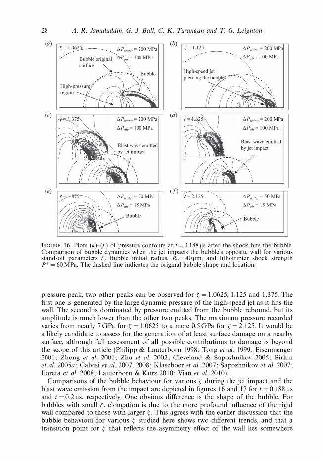
28 A. R. Jamaluddin, G. J. Ball, C. K. Turangan and T. G. Leighton
Bubble originalsurface
Bubble
Blast wave emittedby jet impact
High-speed jet piercing the bubble
High-pressureregion
BubbleBubble
Blast wave emittedby jet impact
�Pwater = 200 MPa
�Pair = 100 MPa
�Pwater = 200 MPa
�Pair = 100 MPa
�Pwater = 200 MPa
�Pair = 100 MPa
�Pwater = 200 MPa
�Pair = 100 MPa
ζ = 1.0625
ζ = 1.375 ζ = 1.625
�Pwater = 50 MPa
�Pair = 15 MPa
�Pwater = 50 MPa
�Pair = 15 MPa
ζ = 1.875 ζ = 2.125
ζ = 1.125(a) (b)
(c) (d)
(e) ( f )
Figure 16. Plots (a)–(f ) of pressure contours at t = 0.188 µs after the shock hits the bubble.Comparison of bubble dynamics when the jet impacts the bubble’s opposite wall for variousstand-off parameters ζ . Bubble initial radius, R0 = 40 µm, and lithotripter shock strengthP + =60 MPa. The dashed line indicates the original bubble shape and location.
pressure peak, two other peaks can be observed for ζ =1.0625, 1.125 and 1.375. Thefirst one is generated by the large dynamic pressure of the high-speed jet as it hits thewall. The second is dominated by pressure emitted from the bubble rebound, but itsamplitude is much lower than the other two peaks. The maximum pressure recordedvaries from nearly 7 GPa for ζ =1.0625 to a mere 0.5 GPa for ζ =2.125. It would bea likely candidate to assess for the generation of at least surface damage on a nearbysurface, although full assessment of all possible contributions to damage is beyondthe scope of this article (Philipp & Lauterborn 1998; Tong et al. 1999; Eisenmenger2001; Zhong et al. 2001; Zhu et al. 2002; Cleveland & Sapozhnikov 2005; Birkinet al. 2005a; Calvisi et al. 2007, 2008; Klaseboer et al. 2007; Sapozhnikov et al. 2007;Iloreta et al. 2008; Lauterborn & Kurz 2010; Vian et al. 2010).
Comparisons of the bubble behaviour for various ζ during the jet impact and theblast wave emission from the impact are depicted in figures 16 and 17 for t = 0.188 µsand t = 0.2 µs, respectively. One obvious difference is the shape of the bubble. Forbubbles with small ζ , elongation is due to the more profound influence of the rigidwall compared to those with larger ζ . This agrees with the earlier discussion that thebubble behaviour for various ζ studied here shows two different trends, and that atransition point for ζ that reflects the asymmetry effect of the wall lies somewhere

The shock-induced bubble collapse in SWL and its far-field acoustic emissions 29
ζ = 1.0625 ζ = 1.125(a) (b)
(c) (d)
(e) ( f )
�Pwater = 100 MPa
�Pair = 50 MPa
�Pwater = 100 MPa�Pair = 50 MPa
ζ = 1.375 ζ = 1.625
ζ = 1.875 ζ = 2.125
�Pwater = 50 MPa
�Pair = 50 MPa
�Pwater = 50 MPa
�Pair = 50 MPa
�Pwater = 50 MPa�Pair = 50 MPa
�Pwater = 50 MPa�Pair = 50 MPa
Bubblefragments
Bubble Bubble
Bubble Bubble
Blast wavefrom jet impact
Blast wave from jet impact
Bubblefragments
Figure 17. Plots (a)–(f ) of pressure contours at t = 0.2 µs after the shock hits the bubble.Comparison of bubble dynamics after the jet impact for various stand-off parameters ζ ,showing an intense blast wave emission. R0 = 40 µm and P + = 60 MPa. The dashed lineindicates the original bubble shape and location. Insets are close-up views.
between 1.125 and 1.375. Below this ζ , the contributory effect from the wall issignificant.
The shape of the jet is narrower in cases 1 and 2 (due to the elongation of thecollapsing bubble associated with its interaction with the reflected incident shock)than in cases 3–6 where the ‘shoulder’ of the jet is broader (figure 16). The circulatingflow near the bubble’s upstream surface creates a concave jet tip, which is highlyprominent for ζ = 1.375 and ζ = 1.625. The jet tip is relatively wide and much flatterin cases 5 and 6.
The moment after the jet impact is shown in figure 17. For cases 1 and 2, thejet has penetrated through the bubble isolating a few toroidal bubble fragments(figure 17a, b). In cases 3–6, as a result of the highly concave jet, the impact ofthe jet on the downstream surface forms a toroidal bubble of highly compressedair and tiny bubble fragments (figure 17c–f ) originating from the air layer trapped

30 A. R. Jamaluddin, G. J. Ball, C. K. Turangan and T. G. Leighton
Kirchhoff far-field pressure emission, Rcs = 0.2 mm
–60 000–40 000–20 000
020 00040 00060 00080 000
Pre
ssur
e (P
a)
Pre
ssur
e (P
a)
Pre
ssur
e (P
a)
P5P4P3P2P1
FWH far-field pressure emission,Rcs = 0.2 mm
–60 000–40 000–20 000
020 00040 00060 00080 000
P5P4P3P2P1
FWH far-field pressure emission of Rcs = 0.20 mm derated by 0.3 dB cm–1 MHz–1
for tissue absorption
–6000
–4000
–2000
0
2000
4000P1
P2
P3
P4
P5
98.3 98.4 98.5 98.6 98.7 98.8 98.9 99.0 99.1 98.3 98.4 98.5 98.6 98.7 98.8 98.9 99.0 99.1
98.3 98.5 98.7 98.9 99.1 99.3 99.5
Time (µs) Time (µs)
Time (µs)
P2
(a)
(c)
(b)
Figure 18. The far-field acoustic emissions read by an observer located at 150mm from theinitial bubble centre for five θ and φ combinations (i.e. observer’s locations denoted by P1–P5 –refer to figure 10). (a) Kirchhoff scheme, (b) FW-H scheme. Stand-off distance ζ =1.0625 andcontrol surface radius Rcs = 0.2 mm, (c) The data of frame (b) derated by the standard valueof 0.3 dB cm−1 MHz−1 to include the effect of absorption in tissue.
between the jet and the downstream interface prior to impact. Of course, undersuch extreme conditions, the details of the air/water interfaces must be treated withcaution, although such predictions are in keeping with experimental observationssuch as the observation of damage rings around jet impact damage pits (Philipp &Lauterborn 1998) and luminescence at the point of jet impact (Bourne & Field 1991;Leighton 1994; Bourne & Milne 2003).
4.3. Far-field acoustic emissions of bubble collapse near a rigid wall
Figure 18 shows the pressure–time history calculated in the far field for ζ =1.0625using the Kirchhoff and FW-H schemes. Results for five different combinations ofθ and φ are plotted for comparison in order to determine the variation in thefar-field pressure profile at different observer positions and the dependency on thedirectionality of the lithotripter shock wave. The same set of integration surfaces andinput data from Vucalm simulations were used for all calculations.
For the case when the rigid wall is present, the incident shock passes twice over thebubble (once travelling from left to right, and then as a reflected wave travelling fromright to left). Therefore, pressure waves directly related to the propagating incidentshock are captured twice in the Kirchhoff and FW-H surface integral. Nevertheless,the blast wave could still be captured as a sharp peak. The timing of the arrivalof the blast wave peak relative to the contamination from the lithotripter shock issuch that there is no overlap. Jamaluddin (2005) demonstrated that the blast wavecan be unambiguously identified from the lithotripter signature by comparing the
The shock-induced bubble collapse in SWL and its far-field acoustic emissions 31
far-field pressure waveforms for the bubble-free cases with those when bubbles arepresent. In figure 18, the large trough for ζ = 1.0625 (P5 line) between 98.6 and98.75 µs can be attributed to the incident shock. The maximum pressure amplitudepredicted for ζ = 1.0625 is approximately 70 kPa. This value decreases by around10 kPa when ζ =2.125. The reduction in the maximum pressure amplitude is becauseof the increase in the distance from the wall of the initial position of the bubblecentre. For ζ =1.0625, the reflection of the blast wave is not very clear. This isbecause the delay between the primary and reflected shocks may be too small toresolve. For ζ =2.125, Jamaluddin (2005) shows that the acoustic emission curvedepicts the second pressure peak owing to the greater distance of the bubble from therigid wall, and that the blast wave has time to develop into a full spherical pressurewave and is reflected by the wall.
The results of the predicted far-field acoustic emission using the FW-H methodare in agreement with that of the Kirchhoff method (figure 18a, b) for all fiveobserver positions. This particular problem has a high degree of flow nonlinearityat any feasible position of the control surface owing to the incident shock wave,its reflection by the rigid wall and the high pressure amplitude of the blast wave.As the FW-H formulation takes into account the flow nonlinearities in the surfaceintegrals, the FW-H method is expected to give more consistent and acceptableresults regardless of the control surface position compared to the Kirchhoff method.The results show that there are negligible differences in the abilities of bothmethods to distinguish the lithotripter signature from the blast wave signature.Therefore, the implementation of both methods warrants exploration in this particularscenario.
Figure 18(c) shows derated versions of the data in figure 18(b) to include the effectof absorption in tissue (as was done to generate figure 11d ). The divergence on theleft of the figure is an artefact. It is not a frequency folding effect (it does not, forexample, occur at the extreme right of the plots) but instead occurs because thederating algorithm is defined in terms of amplitude alone, at 0.3 dB cm−1 MHz−1. Forwant of information to the contrary, a zero-phase response is included with the filter(i.e. a filter that introduces no delays). Such filters are acausal, in that they create anoutput using data before and after the current sample, which produces an unphysicalresult in this case. However, application of an acausal filter in this way is deemedhere to be an appropriate procedure to obtain an estimate of the effect of tissueabsorption, in the absence of specific information on the phase requirements of thefilter. Whilst this effect would in principle have occurred in figure 11(d ), the natureof the signal made it undiscernible.
5. ConclusionsThe jetting collapse of a single bubble in a free field and near a rigid wall for various
stand-off distances due to interaction with a lithotripter shock has been simulatedusing the FLM code. The collapse is asymmetric, forming a high speed jet that impactsthe far bubble wall, generating an intense blast wave. To predict the far-field acousticemissions from the bubble collapse, the time histories of pressure and its derivativesrecorded on a control surface placed inside the FLM computational domain are usedas inputs to the Kirchhoff and FW-H methods. For the control surface radii employedhere (Rcs = 5 R0 = 0.2mm for an initial bubble radius of R0 = 40 µm), both methodsare able to predict the far-field acoustic emissions in water. However, the method isonly accurate if the control surface is placed at a sufficient range from the source

32 A. R. Jamaluddin, G. J. Ball, C. K. Turangan and T. G. Leighton
to ensure that only linear acoustic propagation occurs beyond it; if the CFD field istoo limited for this, an alternative method of nonlinearly propagating the waveformbetween increasingly large control surfaces should be considered. In the currentproject studentship, the computational resources were insufficient to implement eitherapproach. However, the scenario of interest here is to support understanding of aclinical device, and the importance of balancing the tendency of tissue to generatenonlinear waveforms with its ability to absorb the waveform was outlined, and thewaveforms corrected following the standard derating procedure which neglects theeffects of nonlinear propagation. Having demonstrated the technique for predictingthe acoustic emission from single bubbles, the next paper in this series will showhow this is developed to predict the far-field acoustic emissions from single bubblesattached to a wall and from cavitation clouds during SWL.
A. R. Jamaluddin was supported through a PhD studentship provided by theEPSRC (grant no. GR/N19243; Principal Investigator: T. G. Leighton). The authorsare grateful to Prof. P. White for assistance in producing the derated values infigures 11(d ) and 18(c).
REFERENCES
Bailey, M. R., Khokhlova, V. A., Sapozhnikov, O. A., Kargl, S. G. & Crum, L. A. 2003 Physicalmechanisms of the therapeutic effect of ultrasound (a review). Acoust. Phys. 49 (4), 369–388.
Bailey, M. R., Pishchalnikov, Y. A., Sapozhnikov, O. A., Cleveland, R. O., McAteer, J. A.,
Miller, N. A., Pishchalnikova, I. V., Connors, B. A., Crum, L. A. & Evan, A. P. 2005Cavitation detection during shock-wave lithotripsy. Ultrasound Med. Biol. 31 (9), 1245–1256.
Ball, G. J. 1996 A free-Lagrange method for unsteady compressible flow: simulation of a confinedcylindrical blast wave. Shock Waves 5, 311–325.
Ball, G. J., Howell, B. P., Leighton, T. G. & Schofield, M. J. 2000 Shock-induced collapse of acylindrical air cavity in water: a free-Lagrange simulation. Shock Waves 10, 265–276.
Benjamin, T. B. & Ellis, A. T. 1966 The collapse of cavitation bubbles and the pressure therebyproduced against solid boundaries. Phil. Trans. R. Soc. Lond. A 260, 221–240.
Birkin, P. R., Offin, D. G., Joseph, P. F. & Leighton, T. G. 2005a Cavitation, shock waves andthe invasive nature of sonoelectrochemistry. J. Phys. Chem. B 109, 16997–17005.
Birkin, P. R., Offin, D. G. & Leighton, T. G. 2004a Electrochemical measurements of the effectsof inertial acoustic cavitation by means of a novel dual microelectrode. Electrochem. Commun.6 (11), 1174–1179.
Birkin, P. R., Offin, D. G. & Leighton, T. G. 2004b The study of surface processes underelectrochemical control in the presence of inertial cavitation. Wear 258 (1–4), 623–628.
Birkin, P. R., Offin, D. G. & Leighton, T. G. 2005b Experimental and theoretical characterisationof sonochemical cells. Part 2. Cell disruptors (ultrasonic horn) and cavity cluster. J. Phys.Chem. 7, 530–537.
Blake, J. R., Hooton, M. C., Robinson, P. B. & Tong, R. P. 1997 Collapsing cavities, toroidalbubbles and jet impact. Phil. Trans. R. Soc. Lond. A 355, 537–550.
Blake, J. R., Taib, B. B. & Doherty, G. 1986 Transient cavities near boundaries: Part 1. Rigidboundary. J. Fluid Mech. 170, 479–497.
Bouakaz, A., Merks, E., Lance’e, C. & Bom, N. 2004 Noninvasive bladder volume measurementsbased on nonlinear wave distortion. Ultrasound Med. Biol. 30 (4), 469–476.
Bourne, N. K. & Field, J. E. 1991 Bubble collapse and the initiation of explosion. Proc. R. Soc.Lond. A 435, 423–435.
Bourne, N. K. & Field, J. E. 1999 Shock-induced collapse and luminescence by cavities. Proc.R. Soc. Lond. A 357, 295–311.

The shock-induced bubble collapse in SWL and its far-field acoustic emissions 33
Bourne, N. K. & Milne, A. M. 2003 The temperature of shock-collapsed cavity. Proc. R. Soc.Lond. A 459, 1851–1861.
Brentner, K. S. & Farassat, F. 1998 Analytical comparison of the acoustic analogy and Kirchhoffformulation for moving surfaces. AIAA 36 (8), 1379–1386.
Brujan, E. A., Nahen, K., Schmidt, P. & Vogel, A. 2001 Dynamics of laser-induced cavitationbubbles near elastic boundaries: influence of the elastic modulus. J. Fluid. Mech. 433, 283–314.
Burley, M. M., Madsen, E. L., Zagzebski, J. A., Banjavic, R. A. & Sum, S. W. 1980 A newultrasound tissue-equivalent material. Radiology 134, 517–520.
Calvisi, M. L., Iloreta, J. I. & Szeri, A. J. 2008 Dynamics of bubbles near a rigid surface subjectedto a lithotripter shock wave. Part 2. Reflected shock intensifies nonspherical cavitation collapse.J. Fluid. Mech. 616, 63–97.
Calvisi, M. L., Lindau, O., Blake, J. R. & Szeri, A. J. 2007 Shape stability and violent collapse ofmicrobubbles in acoustic traveling waves. Phys. Fluids 19, 047101.
Chaudhri, M. M. & Field, J. E. 1974 The role of rapidly compressed gas pockets in the initiationof condensed explosives. Proc. R. Soc. Lond. A 340, 113–128.
Church, C. C. 1989 A theoretical study of cavitation generated by an extracorporeal shock wavelithotripter. J. Acoust. Soc. Am. 86, 215–227.
Cleveland, R. O. & Sapozhnikov, O. A. 2005 Modelling elastic wave propagation in kidney stoneswith application to shock wave lithotripsy. J. Acoust. Soc. Am. 118 (4), 2667–2676.
Cleveland, R. O., Sapozhnikov, O. A., Bailey, M. R. & Crum, L. A. 2000 A dual passivecavitation detector for localized detection of lithotripsy-induced cavitation in vitro. J. Acoust.Soc. Am. 107, 1745–1758.
Coleman, A. J., Choi, M. J., Saunders, J. E. & Leighton, T. G. 1992 Acoustic emission andsonoluminescence due to cavitation at the beam focus of an electrohydraulic shock wavelithotripter. Ultrasound Med. Biol. 18, 267–281.
Coleman, A. J. & Saunders, J. E. 1989 A survey of the acoustic output of commercial extracorporealshock wave lithotripters. Ultrasound Med. Biol. 15, 213–227.
Coleman, A. J., Saunders, J. E., Crum, L. A. & Dyson, M. 1987 Acoustic cavitation generated byan extracorporeal shock-wave lithotripter. Ultrasound Med. Biol. 13, 69–76.
Coleman, A. J., Whitlock, M., Leighton, T. G. & Saunders, J. E. 1993 The spatial distribution ofcavitation induced acoustic emission, sonoluminescence and cell lysis in the field of a shockwave lithotripter. Phys. Med. Biol. 38, 1545–1560.
Coley, G. D. & Field, J. E. 1973 The role of cavities in the initiation and growth of explosion inliquids. Proc. R. Soc. Lond. A 335, 67–86.
Cooter, R. D., Babidge, W. J., Mutimer, K., Wickham, P., Robinson, D., Kiroff, G., Chapman,
A. & Madden, G. J. 2001 Ultrasound-assisted lipoplasty. Austral. NZ J. Surg. 71 (5), 309–317.
Coussios, C. C. & Roy, R. A. 2008 Applications of acoustics and cavitation to noninvasive therapyand drug delivery. Annu. Rev. Fluid Mech. 40, 395–420.
Cui, J. Y., Hamilton, M. F., Wilson, P. S. & Zabolotskaya, E. A. 2006 Bubble pulsations betweenparallel plates. J. Accoust. Soc. Am. 119 (4), 2067–2072.
Cunningham, K. B., Coleman, A. J., Leighton, T. G. & White, P. R. 2001 Characterising in vivoacoustic cavitation during lithotripsy with time-frequency methods. Acoust. Bull. 26 (5), 10–16.
Damianou, C. A., Sanghvi, N. T. & Fry, F. J. 1997 Dependence of ultrasonic attenuation andabsorption in dog soft tissue on temperature and thermal dose. J. Acoust. Soc. Am. 102 (1),628–634.
Dear, J. P. & Field, J. E. 1988 High-speed photography of surface geometry effects in liquid/solidimpact. J. Appl. Phys. 63, 1015–1021.
Dear, J. P., Field, J. E. & Walton, A. J. 1988 Gas compression and jet formation in cavitiescollapsed by a shock wave. Nature 332, 505–508.
Delius, M. 2000 History of shock wave lithotripsy. In Proceedings of the 15th InternationalSymposium on Nonlinear Acoustics at the Turn of the Millenium , vol. 524, pp. 23–32.
Delius, M. & Gambihler, S. 1992 Sonographic imaging of extracorporeal shock wave effects inthe liver and gallbladder of dogs. Digestion 52, 55–60.
DH 2004 In The NHS Improvement Plan: Putting People at the Heart of Public Services , p. 80. UKDept. of Health Publication Cm 6268, 24 June 2004, Stationary Office, London.

34 A. R. Jamaluddin, G. J. Ball, C. K. Turangan and T. G. Leighton
Ding, Z. & Gracewski, S. M. 1996 The behaviour of a gas cavity impacted by a weak or strongshock wave. J. Fluid Mech. 309, 183–209.
Duck, F. 2010 Tissue nonlinearity. Proc. Inst. Mech. Engrs, Part H: J. Engng. in Med. 224 (2),155–170.
Eisenmenger, W. 2001 The mechanisms of stone fragmentation in ESWL. Ultrasound Med. Biol. 27(5), 683–693.
Farassat, F. & Myers, M. K. 1988 Extension of Kirchhoff’s formula to radiation from movingsurfaces. J. Sound Vib. 123 (3), 451–461.
Farassat, F. & Succi, G. P. 1983 The prediction of helicopter descrete frequency noise. Vertica 7(4), 309–320.
Fedele, F. 2008 Acoustic sensing of renal stones fragmentation in extracorporeal shockwavelithotripsy. PhD thesis, University of Southampton, UK.
Fedele, F., Coleman, A. J., White, P. R. & Hurrell, A. M. 2004 Development of a new diagnosticsensor for extra-corporeal shock-wave lithotripsy. Proceedings of the First Conference onAdvanced Metrology for Ultrasound in Medicine. J. Phys.: Conf. Ser., 134–139.
Fedele, F., Thomas, K., Leighton, T. G., Ryves, S., Phillips, D. & Coleman, A. J. 2010 A passiveacoustic monitor of treatment effectiveness during extracorporeal lithotripsy. Proceedings ofthe Second Conference on Advanced Metrology for Ultrasound in Medicine. J. Phys.: Conf.Ser . 279, 1–6.
Field, J. E. 1994 Experimental studies of bubble collapse. In Bubble Dynamics and InterfacePhenomena (ed. J. R. Blake), pp. 17–31. Kluwer Academic.
Field, J. E., Swallowe, G. M. & Heavens, S. N. 1982 Ignition mechanisms of explosives duringmechanical deformation. Proc. R. Soc. Lond. A 383, 231–244.
Fong, S. W., Klaseboer, E., Turangan, C. K., Khoo, B. C. & Hung, K. C. 2006 Numerical analysisof a gas bubble near bio-materials in an ultrasound field. Ultrasound Med. Biol. 32, 925–942.
di Francescantonio, P. 1997 A new boundary integral formulation for the prediction of soundradiation. J. Sound Vib. 202 (4), 491–509.
Freund, J. B. 2008 Suppression of shocked-bubble expansion due to tissue confinement withapplication to shock-wave lithotripsy. J. Acoust. Soc. Am. 123 (5), 2867–2874.
Gao, F. R., Hu, Y. T. & Hu, H. P. 2007 Asymmetrical oscillation of a bubble confined inside a micropseudoelastic blood vessel and the corresponding vessel wall stresses. Intl J. Solid Struct. 44(22–23), 7197–7212.
Gol’dberg 1956 Second approximation acoustic equations and the propagation of plane waves offinite amplitude. Sov. Phys. Acoust. 2, 346–350.
Goss, S. A., Johnston, R. L. & Dunn, F. 1980 Compilation of empirical ultrasound properties ofmammalian tissues. Part II. J. Acoust. Soc. Am. 68 (1), 93–108.
Hamilton, M. F. & Blackstock, D. T. 1998 In Nonlinear Acoustics, Theory and Applications , p. 102.Academic Press.
Haran, M. E. & Cook, B. D. 1983 Distortion of finite amplitude ultrasound in lossy media.J. Acoust. Soc. Am. 73, 774–779.
Hirsimaki, H. M., Birkin, P. R., Frey, J. G. & Leighton, T. G. 2006 The laser-induced formationof plasma bubbles in water–electrochemical measurements. Proc. Inst. Acoust. 28 (1), 876–884.
Howell, B. P. & Ball, G. J. 2000 Damping of mesh-induced errors in free-Lagrange simulationsof Richtmyer–Meshkov instability. Shock Waves 10, 253–264.
Howell, B. P. & Ball, G. J. 2002 A free-Lagrange augmented Godunov method for the simulationof elastic–plastic solids. J. Comput. Phys. 175, 128–167.
Iloreta, J. I., Fung, N. & Szeri, A. J. 2008 Dynamics of bubbles near a rigid surface subjected toa lithotripter shock wave. Part 1. Consequences of interference between incident and reflectedwaves. J. Fluid Mech. 616, 43–61.
Jamaluddin, A. R. 2005 Free-Lagrange simulations of shock–bubble interaction in extracorporealshock wave lithotripsy. PhD thesis, University of Southampton, U.K.
Jamaluddin, A. R., Ball, G. J. & Leighton, T. G. 2002 Free-Lagrange simulations of shock/bubbleinteraction in shock wave lithotripsy. In Proceedings of the Second International Conferenceon Computational Fluid Dynamics (ICCFD), Sydney, Australia, pp. 541–546.
Jamaluddin, A. R., Ball, G. J. & Leighton, T. G. 2004 Free-Lagrange simulations of shock/bubbleinteraction in shock wave lithotripsy. In Proceedings of the 24th International Symposium onShock Waves, Beijing, China, pp. 1211–1216.

The shock-induced bubble collapse in SWL and its far-field acoustic emissions 35
Jarvinen, T. A., Jarvinen, T. L., Kaariainen, M., Kalimo, H. & Jarvinen, M. 2005 Muscle injuries:Biology and treatment. Am. J. Sports Med. 33 (5), 745–764.
Johnsen, E. & Colonius, T. 2009 Numerical simulations of non-spherical bubble collapse. J. FluidMech. 629, 231–262.
Kendrinskii, V. K. 1997 The role of cavitation effects in the mechanisms of destruction andexplosive process. Shock Waves 7, 63–76.
Klaseboer, E., Fong, S. W., Turangan, C. K., Khoo, B. C., Szeri, A. J., Calvisi, M. L., Sankin,
G. N. & Zhong, P. 2007 Interaction of lithotripter shockwaves with single inertial cavitationbubbles. J. Fluid Mech. 593, 33–56.
Klaseboer, E., Turangan, C. K., Fong, S. W., Liu, T. G., Hung, K. C. & Khoo, B. C. 2006Simulations of pressure–pulse bubble interaction using boundary element method. Comput.Meth. Appl. Engng 195, 4287–4302.
Kornfeld, M. & Suvorov, L. 1944 On the destructive action of cavitation. J. Appl. Phys. 15,495–506.
Kuwahara, M., Ioritani, N., Kambe, K., Shirai, S., Taguchi, K., Saitoh, T., Orikasa, S., Takayama,
K., Aida, S. & Iwama, N 1989 Hyperechoic region induced by focused shock waves in vitroand in vivo: Possibility of acoustic cavitation bubbles. J. Lithotripsy Stone Dis. 1, 282–288.
Lauterborn, W. 1972 High-speed photography of laser-induced breakdown in liquids. Appl. Phys.Lett. 21, 27.
Lauterborn, W. & Kurz, T. 2010 Physics of bubble oscillations. Rep. Prog. Phys. 73 (10),106501.
Lea, S. C., Price, G. J. & Walmsley, A. D. 2005 A study to determine whether cavitation occursaround dental ultrasonic scaling instruments. Ultrason. Chem. 12 (3), 233–236.
Leighton, T. G. 1994 In The Acoustic Bubble. The Academic Press.
Leighton, T. G. 2004 From seas to surgeries, from babbling brooks to baby scans: The acousticsof gas bubbles in liquids. Intl J. Mod. Phys. B 18, 3267–3314.
Leighton, T. G. 2007 What is ultrasound? Prog. Biophys. Mol. Biol. 93 (1–3), 3–83.
Leighton, T. G., Birkin, P. R., Hodnett, M., Zeqiri, B., Power, J. F., Price, G. J., Mason,
T., Plattes, M., Dezkunov, N. & Coleman, A. J. 2005 Charaterisation of measures ofreference acoustic cavitation (comorac): An experimental feasibility trial. In Bubble andParticle Dynamics in Acoustic Fields: Modern Trends and Applications (ed. A. A. Doinikov),pp. 37–94. Research Signpost.
Leighton, T. G. & Cleveland, R. O. 2010 Lithotripsy. In Proceedings of the Institute of Mechanical.Engrs, Part H. J. Engng. Med. 224 (2), 317–342.
Leighton, T. G., Cox, B. T. & Phelps, A. D. 2000 The Rayleigh-like collapse of a conical bubble.J. Acoust. Soc. Am. 107 (1), 130–142.
Leighton, T. G., Farhat, M., Field, J. E. & Avellan, F. 2003 Cavitation luminescence from flowover a hydrofoil in a cavitation tunnel. J. Fluid Mech. 480, 43–60.
Leighton, T. G., Fedele, F., Coleman, A. J., McCarthy, C., Jamaluddin, A. R., Turangan,
C. K., Ball, G. J., Ryves, S., Hurrell, A. M., Stefano, A. De & White, P. R. 2008a Thedevelopment of a passive acoustic device for monitoring the effectiveness of shock wavelithotripsy in real time. Hydroacoustics 11, 159–180.
Leighton, T. G., Fedele, F., Coleman, A. J., McCarthy, C., Ryves, S., Hurrell, A. M., Stefano,
A. De & White, P. R. 2008b Clinical studies of a real-time monitoring of lithotripterperformance using passive acoustic sensors. In Proceedings of the Second InternationalUrolithiasis Research Symposium , Indianapolis, USA, pp. 256–277.
Leighton, T. G., Fedele, F., Coleman, A. J., McCarthy, C., Ryves, S., Hurrell, A. M., Stefano,
A. De & White, P. R. 2008c A passive acoustic device for real-time monitoring the efficacyof shockwave lithotripsy treatment. Ultrasound Med. Biol. 34 (10), 1651–1665.
Leighton, T. G., Ho, W. L. & Flaxman, R. 1997 Sonoluminescence from the unstable collapse ofa conical bubble. Ultrasonics 35, 399–405.
Leighton, T. G., Phelps, A. D., Cox, B. T. & Ho, W. L. 1998 Theory and preliminary measurementsof the Rayleigh-like collapse of a conical bubble. Acustica with Acta Acustica 84 (6), 1014–1024.
Leighton, T. G., White, P. R. & Marsden, M. A. 1995a Applications of one-dimensional bubblesto lithotripsy, and to diver response to low frequency sound. Acta Acustica 3, 517–529.

36 A. R. Jamaluddin, G. J. Ball, C. K. Turangan and T. G. Leighton
Leighton, T. G., White, P. R. & Marsden, M. A. 1995b The one-dimensional bubble: An unusualoscillator, with applications to human bioeffects of underwater sound. Eur. J. Phys. 16,275–281.
Lindau, O. & Lauterborn, W. 2003 Cinematographic observation of the collapse and rebound ofa laser-produced cavitation bubble near a wall. J. Fluid Mech. 479, 327–348.
Lingeman, J. E., McAteer, J. A., Gnessin, E. & Evan, P. 2009 Shock wave lithotripsy: advances intechnology and technique. Nat. Rev. Urol. 6, 660–670.
Liu, X., Li, J., Gong, X. & Zhang, D. 2006 Nonlinear absorption in biological tissue for highintensity focused ultrasound. Ultrasonics 44, e27–e30.
Lyrintzis, A. S. & George, A. R. 1989 Use of the Kirchhoff method in acoustics. AIAA J. 27 (10),1451–1453.
Lyrintzis, A. S. & Xue, Y. 1991 Study of the noise mechanisms of transonic blade–vortexinteractions. AIAA J. 29 (10), 1562–1572.
van der Meulen, J. H. J. 1986a On correlating erosion and luminescence from cavitation on adydrofoil. In Proceedings of the International Symposium on Propellers and Cavitation , pp. 13–19.
van der Meulen, J. H. J. 1986b The relation between noise and luminescence from cavitationon a hydrofoil. In Joint ACSE/ASME Conference on Cavitation in Hydraulic Structures andTurbomachinery (ed. R. E. A. Arndt & D. R. Web), pp. 149–159.
O’Brien, W., Yang, Y. & Simpson, D. 2004 Evaluation of unscanned-mode soft-tissue thermal indexfor rectangular sources and proposed new indices. Ultrasound Med. Biol. 30 (7), 965–972.
Ohl, C. D., Kurz, T., Geisler, R., Lindau, O. & Lauterborn, W. 1999 Bubble dynamics, shockwaves and sonoluminescence. Phil. Trans. R. Soc. Lond. A 357, 269–294.
O’Leary, R., Sved, A. M., Davies, E. H., Leighton, T. G., Wilson, T. G. & Kieser, J. B.
1997 The bacterial effects of dental ultrasound on Actinobacillus Actiomycetemcomitans andPorphyromonas Gingivalis – an in vitro investigation. J. Clin. Periodontol. 24, 432–439.
Philipp, A. & Lauterborn, W. 1998 Cavitation erosion by single laser-produced bubbles. J. FluidMech. 361, 75–116.
Sankin, G. N., Simmons, W. N., Zhu, S. L. & Zhong, P. 2005 Shockwave interaction with lasergenerated single bubbles. Phys. Rev. Lett. 95, 034501.
Sapozhnikov, O. A., Maxwell, A. D., MacConaghy, B. & Bailey, M. R. 2007 A mechanisticanalysis of stone fracture in lithotripsy. J. Acoust. Soc. Am. 121, 1190–1202.
Sassaroli, E. & Hynynen, K. 2007 Cavitation threshold of microbubbles in gel tunnels by focusedultrasound. Ultrasound Med. Biol. 33 (10), 1651–1660.
Shima, A. 1997 Studies of bubble dynamics. Shock Waves 7, 33–42.
Smith, N. C., Fedele, F., Leighton, T. G., Coleman, A. J. & Thomas, K. 2009 The ‘SmartStethoscope’: Predicting the outcome of lithotripsy Abstract. BJU Intl (formerly: Br. J. Urol.)103 (4), pp. 32.
Takayama, K. 1999 Application of shock wave research to medicine. In Proceedings of the 22ndInternational Symposium on Shock Waves, London, UK, pp. 23–32.
Tomita, Y. & Shima, A. 1986 Mechanisms of impulsive pressure generation and damage pitformation by bubble collapse. J. Fluid Mech. 169, 535–564.
Tong, R. P., Schiffers, W. P., Shaw, S. J., Blake, J. R. & Emmony, D. C. 1999 The role of‘splashing’ in the collapse of a laser-generated cavity near a rigid boundary. J. Fluid Mech.380, 339–361.
Turangan, C. K. 2004 Free-Lagrange simulations of cavitation bubble collapse. PhD thesis,University of Southampton, U.K.
Turangan, C. K., Jamaluddin, A. R., Ball, G. J. & Leighton, T. G. 2008 Free-Lagrange simulationsof the expansion and jetting collapse of air bubbles in water. J. Fluid Mech. 598, 1–25.
Turangan, C. K., Ong, G. P., Klaseboer, E. & Khoo, B. C. 2006 Experimental and numericalstudy of transient bubble–elastic membrane interaction. J. Appl. Phys. 100, 054910.
Vian, C. J. B., Birkin, P. R. & Leighton, T. G. 2010 Cluster collapse in a cylindrical cell:Correlating multibubble sonoluminescence, acoustic pressure and erosion. J. Phys. Chem. C114 (39), 16416–16425.
Vogel, A., Lauterborn, W. & Timm, R. 1989 Optical and acoustic investigations of the dynamicsof laser-produced cavitation bubbles near a solid boundary. J. Fluid Mech. 206, 299–338.

The shock-induced bubble collapse in SWL and its far-field acoustic emissions 37
Whittingham, T. 2007 Wfumb safety symposium on echo-contrast agents: Exposure from diagnosticultrasound equipment relating to cavitation risk. Ultrasound Med. Biol. 33 (2), 214–223.
Zderic, V., Keshavarzi, A., Andrew, M. A., Vaezy, S. & Martini, R. W. 2004 Attenuation ofporcine tissues in vivo after high intensity ultrasound treatment. Ultrasound Med. Biol. 30 (1),61–66.
Zequiri, B., Hodnett, M. & Leighton, T. G. 1997 A strategy for the development andstandardisation of measurement methods for high power/cavitating ultrasound fields – finalproject report. Tech. Rep., NPL Rep. CIRA(EXT)016.
Zhong, P., Cioanta, I., Cocks, F. H. & Preminger, G. M. 1997 Inertial cavitation and associatedacoustic emission produced during electrohydraulic shock wave lithotripsy. J. Acoust. Soc.Am. 101 (5 Pt 1), 2940–2950.
Zhong, P., Zhou, Y. & Zhu, S. 2001 Dynamics of bubble oscillations in constrained media andmechanisms of vessel rupture in swl. Ultrasound Med. Biol. 27, 119–134.
Zhu, S. L., Cocks, F. H., Preminger, G. M. & Zhong, P. 2002 The role of stress waves andcavitation in stone comminution in shock wave lithotripsy. Ultrasound Med. Biol. 27, 661–671.