38

THE CO-EMERGENCE OF AGGREGATE AND MODELLING REASONING1

KEREN ARIDOR

LINKS I-CORE, University of Haifa, Israel Keren.aridor@gmail.com

DANI BEN-ZVI

LINKS I-CORE, University of Haifa, Israel dbenzvi@univ.haifa.ac.il

ABSTRACT

This article examines how two processes – reasoning with statistical modelling of

a real phenomenon and aggregate reasoning – can co-emerge. We focus in this case study on the emergent reasoning of two fifth graders (aged 10) involved in statistical data analysis, informal inference, and modelling activities using TinkerPlotsTM. We describe nine phases of the students’ articulations of aggregate and modelling reasoning as they explored a small sample, constructed a model and generated random samples from this model to examine its validity. These phases are distinguished by the students’ views toward data, variability, and models. We discuss implications and limitations of the results. Despite the idiosyncrasy of the case, the lessons are important because they open a new direction for research about reasoning with data and models.

Keywords: Aggregate reasoning; Exploratory data analysis; Informal statistical

inference; Statistical model and modelling; Statistics education research

1. INTRODUCTION

One of the core aspects of statistical reasoning is handling data from an aggregate point of view (Hancock, Kaput, & Goldsmith, 1992), namely, viewing data as an entity with emergent properties, such as shape, center, and spread (Konold, Higgins, Russell, & Khalil, 2014). Young students tend to see data as individual cases and measurement values as inseparable from an object or person measured. Students who cannot develop a notion of an organizing structure with which they can see the whole instead of just the elements miss the essential point of doing statistics, which is predicting properties of aggregates (Bakker & Hoffmann, 2005). Therefore, developing students’ aggregate view of data is a key challenge in statistics education (Bakker, Biehler, & Konold, 2004). Placing data modelling at the heart of statistics learning can address this challenge by prompting students to search for patterns in data and to account for variability in those patterns (Pfannkuch & Wild, 2004). Data modelling processes themselves entail aggregate reasoning processes (Lehrer & Schauble, 2015). In this article, we study the co-emergence of aggregate and modelling reasoning processes. This case study is part of a UK-Israel research project aimed at developing and studying a modelling approach for teaching and learning statistics (Ainley, Aridor, Ben-Zvi, Manor, & Pratt, 2013; Ainley & Pratt, 2014). We concentrate here on how fifth graders’ modelling of an authentic phenomenon using TinkerPlotsTM (Konold & Miller, 2011) supported the articulation of co-emerging aggregate reasoning and reasoning

Statistics Education Research Journal, 16(2), 38-63, http://iase-web.org/Publications.php?p=SERJ International Association for Statistical Education (IASE/ISI), November, 2017

39

with modelling. We focus on the way they articulated their reasoning with models and modelling and the shift between local and aggregate views of data.

We start by reviewing relevant theoretical background on informal statistical reasoning, aggregate reasoning, reasoning with variability, modelling, exploratory data analysis and Active Graphing. In Section 3, we present the methodology, the pedagogical approaches that guided the design of the intervention, and the Dalmatians Task. Next, we present the main results of this research in the form of nine primary phases through which the students’ statistical reasoning coevolved between aggregate and modeling approaches. We conclude with theoretical and pedagogical implications and limitations of the research.

2. SCIENTIFIC BACKGROUND

2.1. INFORMAL STATISTICAL INFERENCE

Informal Statistical Inference (ISI) is a relatively new view of teaching statistics that

embraces informal ways of making inferences (Maker & Rubin, 2009). Teaching ISI aims at deepening learners’ understanding of the key ideas of statistical inference in relation to other key statistical ideas (Garfield & Ben-Zvi, 2008). ISI is based on making generalizations beyond the given data, expressing uncertainty with a probabilistic language and using data as evidence for those generalizations. The methods of ISI, unlike formal statistical inference that uses formulas and procedures, need not necessarily be the standard methods accepted by the statistics community (Makar & Rubin, 2009). The reasoning process leading to making ISIs is termed Informal Inferential Reasoning (IIR, Makar, Bakker, & Ben-Zvi, 2011). IIR is a cognitive activity that involves formulating generalizations (e.g., conclusions, predictions) about “some wider universe” from random samples of data using various statistical tools, while considering and articulating evidence and uncertainty (Ben-Zvi, Gil, & Apel, 2007). IIR includes reasoning with several key statistical ideas such as: sample size, sampling variability, controlling for bias, uncertainty, and properties of data aggregates (Rubin, Hammerman, & Konold, 2006). 2.2. AGGREGATE REASONING

Developing statistical reasoning involves moving beyond a local view of data toward

a global view of data, and the ability to shift flexibly between these views according to the need and the purpose of the investigation (Ben-Zvi & Arcavi, 2001; Konold et al., 2014). A global view of data is called aggregate reasoning (Konold, Pollatsek, & Well, 1997). When viewing data as an aggregate, a data set is considered as an entity, or as a group with emergent properties, which are different from the properties of the individual cases themselves (Friel, 2007). Konold et al. (2014) defined a hierarchy of three other perspectives of viewing data that differ from an aggregate view: 1. Data as pointers to the context of the data source without referring to the data

themselves. Data cases serve as reminders of the larger event from which they came (e.g., referring to events that happened during the data collection that are not necessarily seen in the data).

2. Data as case values that provide information about the value of some attribute for each individual case (e.g., focusing on extreme values).

3. Data as classifiers that give information about the frequency of cases with a particular attribute value. Such cases are perceived as a unit with similar properties (e.g., the mode of the data).

40

The notion of distribution as an organizing conceptual structure is supported by aggregate reasoning (Bakker & Gravemeijer, 2004) that concentrates on the distribution’s features such as: the general shape, how spread out the cases are, and where the cases tend to be concentrated within the distribution (Konold et al., 2014). Aggregate reasoning with categorical data might refer to frequencies using percentage or quantitative descriptors (e.g., “most”, “majority”), and with numeric data, it might relate to measures of center (i.e., mean, median), shape (e.g., symmetry, skewness), density (actual or relative frequency, majority, quartiles) and spread (e.g., outliers, range, interquartile range, standard deviation) (Cobb, 1999; Friel, 2007). Two important properties of aggregate reasoning are: 1) distinctions between signal and noise; 2) recognition and diagnosis of various types and sources of variability (e.g., natural variability, variability due to measurement error, sampling variability) (Rubin et al., 2006).

2.3. REASONING WITH VARIABILITY

Variability means that something is apt or liable to vary or change (Reading &

Shaughnessy, 2004). When reasoning with data, two types of variability are considered: the “real” variability, which is a characteristic of the phenomenon and an “induced” variability resulting from data collection (measurements, sampling, and accident). Responses to variability are varied. Variability can be “ignored” or considered nonexistent by describing every object in the phenomenon as the same or different in some deterministically known way. Variability can be “allowed for” and described using conditions for its existence. Finally, variability can be “controlled” by trying to change patterns to something more desirable, for example, by isolating causes (Wild & Pfannkuch, 1999).

The search for sources of variability in data entails looking for patterns and relationships between variables: “regularities.” When no regularities are found, variability can only be estimated globally. When some regularities are found but their causes cannot be explained or cannot be manipulated, variability might be estimated locally by measures of variability that are relevant for individual cases. When it is possible to explain and manipulate regularities’ causes, controlling variability can be considered. The more we are able to explain regularities’ causes, the higher the confidence in our ability to predict from data (Wild & Pfannkuch, 1999).

A signal is a constant cause, or a stable property of a variable system, such as the mean or line of fit. It can become evident only in the aggregate. Noise can be considered as variable causes that serve to introduce variability around any signal (Rubin et al., 2006). The signal can be considered as the “explained” variability and the noise as “unexplained” variability (Wild & Pfannkuch, 1999). One can think about a signal in a noisy process as the certainty in situations involving uncertainty (Konold & Pollatsek, 2002). Modelling a phenomenon entails the search for differences and similarities within the population attributes, which is an initial step toward reasoning with variability (Lehrer & Schauble, 2012).

2.4. MODELS AND MODELLING

In general, modelling is considered a form of explanation that is characteristic – even

defining – of science (Lehrer & Schauble, 2010). It is a process of forming a simplification of a phenomenon (the model) on the basis of key theoretical aspects and data in a particular discipline, as well as evaluating and improving it to include theoretical ideas or new findings (Lesh, Carmona, & Post, 2002). Modelling reasoning entails deliberately and

41

temporarily turning attention away from the investigated phenomenon to construct a model (Lehrer & Schauble). In this study, we term reasoning with models (artifacts) and modelling (process) as “reasoning with modelling”, or as “modelling reasoning”.

Mathematical models are abstract constructs that focus on structural characteristics or on a general pattern that is common to several systems (Lesh & Harel, 2003). In statistics, mathematical models are used to represent a general pattern of the data (Moore, 1990). A model can be defined as an analogy that simplifies a real phenomenon and describes some of the connections and relations among its components. A model can be formed by observing a real phenomenon and selecting and focusing on features that are relevant to a specific purpose for which it was constructed. It might be abstract (conceptual) or concrete (e.g., graph, table, dice). The abstract model can represent a real-world system and the conjectures about it in order to describe, explain, predict, and elaborate on its behavior (Lehrer & Schauble, 2010; Wild & Pfannkuch, 1999). A concrete model can serve as a tool for a) representing a process, such as a production of the population, its key components or properties through prediction or by sampling; and b) making an inference about the representativeness of a random sample (as in this case study).

Models can be classified as static or dynamic. A static model is one that does not generate data. It is constructed to describe the population or predict its behavior. A dynamic model is one that can generate random data (a simulation), in order to answer questions about the model’s validity, representativeness of a random sample, etc. Students’ transitions between static models and dynamic models can support their reasoning with the representativeness of random samples (Manor Braham & Ben-Zvi, 2017).

Models and modelling are essential elements of statistical reasoning and thinking (Wild & Pfannkuch, 1999). The practice of statistics can be considered a form of modelling, as the development of models of data, variability and chance pave the way for statistical investigation (Lehrer, Kim, Ayers, & Wilson, 2014). Modelling may support the emergence of students’ informal statistical ideas (Garfield & Ben-Zvi, 2008). The developmental modelling process begins with making sense of a phenomenon and deciding what its important elements are and how they can be measured. Next, data are structured, organized, and visualized, and efforts are made to aggregate data in various ways according to different purposes and to make inferences about the world. This process might inspire more modelling cycles, questioning new epistemic ideas (Lehrer & Schauble, 2000; 2004).

A pedagogical modelling approach puts the modelling process (along with learning about the nature and the purposes of models) in the center of the learning process (Schwartz & White, 2005). Such an approach can support learners in coordinating their understanding of particular cases with an evolving notion of data as an aggregate of cases (Lehrer & Schauble, 2004). This can be achieved, among other ways, by recognizing the need to summarize and represent data in multiple ways depending on their nature (Pfannkuch & Wild, 2004). A pedagogical modelling approach that views real data as a source for a model of a situation in the real world can serve as a bridge between data and probability (Hancock et al., 1992; Konold & Kazak, 2008) by: a) providing multiple affordances to learn about random samples and sampling from an investigated population; b) encouraging consideration of key statistical ideas emanating from the study of a hypothetical model of this population; c) prompting examination of the connections between these elements (Manor Braham, Ben-Zvi, & Aridor, 2013). For example, modelling a random behavior might provide an opportunity to experience and reflect upon probabilistic situations. It allows mimicking such behavior in a real world system, answering questions about that system, and making predictions of future outcomes. Modelling random behavior underpins the quantification of uncertainty using statistical inference techniques such as confidence intervals and significance testing (Arnold, Budgett, & Pfannkuch, 2013).

42

In this case study, several models (e.g., conjectures, predictions, TinkerPlotsTM graphs, and Sampler's models) were developed by a pair of students in an attempt to describe a real phenomenon, make predictions about it, and “produce” its population. We focus on the emergence of reasoning with these models in relation to students’ views of data, in the context of two educational approaches: Exploratory Data Analysis (Tukey, 1977) and Active Graphing (Ainley, Nardi, & Pratt, 2000). 2.5. EXPLORATORY DATA ANALYSIS AND ACTIVE GRAPHING

Exploratory data analysis (EDA), developed first by Tukey (1977), is an accepted way of approaching the analysis of data (Biehler, 1990). EDA can help develop students’ statistical reasoning as they collect, organize, describe and analyse data, with emphasis on simple sense-making tools and visual representations, usually with the aid of technology, for interpretation, analysis, and inference (Moore, 1997). Making sense of data in their context includes clarifying the reasons and purposes for collecting the data, recognizing patterns and trends, formulating conjectures, and explaining and drawing informal inferences (Pfannkuch, Rubick, & Yoon, 2002). These complex processes require the abilities to create and interpret graphs, which can be challenging for students (Ainley, Pratt, & Nardi, 2001).

Active Graphing (AG) is a pedagogic strategy developed by Ainley and Pratt (Ainley et al., 2001) to support students’ understanding of graphs. Students are involved in an investigative process requiring them to use graphs (created with technology) to solve meaningful problems. During this process, students need to be aware of the dependent relationship between variables, and to collect, organize and analyse small amounts of data in order to decide about their next step in the experiment. Ideally, this process includes several iterations of data collection and graphing. The necessity of making sense of graphs during this process encourages students to perceive the graph as an analytical tool rather than just as a tool for data representation (Ainley et al., 2000). In the current task design, we used modelling as a bridge to integrate EDA and AG (Ainley et al., 2013).

This literature review is a brief description of the main statistical ideas that underlie the current research. We elaborated on each of the concepts and the challenges that might occur as students' reason about them. In the next section, we present our research question and the research method and setting in order to put these ideas in the context of the current study.

3. METHOD

3.1. THE RESEARCH QUESTION

In this case study, we focus on two fifth-grade students who were involved in making

informal statistical inferences and modelling. In this context, we ask: How can students’ aggregate reasoning and reasoning with modelling co-emerge?

3.2. THE SETTING AND PARTICIPANTS

In order to address this question, we use data from a pair of fifth-grade students (age

10) as they participated in the Dalmatians Task – an authentic inquiry of exploration, prediction, and explanation of statistical models in the context of ISI. This case study is a part of a UK-Israel collaboration (2012-2014) aimed at developing and studying a modelling approach for teaching and learning statistics by integrating the benefits of

43

Exploratory Data Analysis (EDA) and Active Graphing (AG) (Ainley et al., 2013; Ainley & Pratt, 2014). Constructing a model that would reflect the investigated data and produce a realistic population, along with the use of EDA and AG, addressed the students’ need for purpose and utility (Ainley & Pratt, 2002).

The participants were Iddo and Yael, a pair of academically successful and articulate ten-year-olds (Grade 5) from two Israeli public schools. Both students had high achievement in mathematics. They were communicative students who felt comfortable to share their thoughts, beliefs and doubts, and to explain their opinions in case of a conflict in order to reach consensus. Both students studied earlier during the school year how to calculate the arithmetic mean. Other than that, they had no previous formal experience in statistics or TinkerPlotsTM. The students agreed to participate in this study, and they spent three consecutive hours on the Dalmatians Task.

Two researchers (the first author and a statistics education researcher) introduced the task and the tools and frequently asked the students to clarify their reasoning. One of them presented the task and TinkerPlotsTM to the students and the other focused mostly on documentation (recording video and taking notes). TinkerPlotsTM was briefly introduced to them by inviting them to experiment with the tool’s interface. For each tool or action that the students generated, the researcher briefly described its function. In some cases, the researcher offered to add another tool or to extend the action without directing the students to construct a certain representation or device (e.g., “you can drag upward to further separate the attribute”). When the TinkerPlotsTM Sampler (a tool to model probabilistic processes and generate simulated data from them, Konold & Miller, 2011) was presented, the researcher described each device, besides the counter, while the students experienced it. The option to add dependency between attributes in the Sampler was presented to them only after they had tried to invent methods to handle dependency. In this setting, the students were encouraged to explore data openly, mixing and generating representations that they found interesting and useful, with minor support from the researchers.

3.3. THE DALMATIANS TASK

The children were asked to construct a model (a “machine”, as we termed the Sampler

model) that would “produce” realistic Dalmatian dogs of different sizes in order to create a theme park for the 101 Dalmatians movie. They were asked to base the model on a data sample (Figure 1). The sample size was selected to be small in order to encourage the students to interpolate and extrapolate while engaging in AG. The values of the quantitative variables were similar to the body measures of real Dalmatians: body length was similar to height at shoulder, leg length was between half and two thirds of height at shoulder, and tail length was a bit more than half body length.

Figure 1. A realistic data set of five Dalmatians in a TinkerPlotsTM table

spots height tail_length body_length leg_length

1

2

3

4

5

brown 41 23 40 22

black 37 23 37 18

black 26 13 27 14

black 30 19 30 16

black 30 15 31 17

44

The actual learning trajectory, which we describe in Table 1, was designed to encourage the students to reason informally and openly with key statistical ideas (such as distribution, center and variability as signal and noise, models, and sample and sampling), express uncertainty, and develop an aggregate view of data, with little help from the researchers.

Table 1. The Dalmatians Task actual learning trajectory

Content Min. Part I: Context and data worlds a) Introduce and discuss the Dalmatians Task: Learn about the task and make

conjectures about the dog population. 5

b) Collect real data: Measure two real Labradors (a breed that is somewhat similar to Dalmatians in size): Julie – eight months old, and Sandy – two years old, and discuss their properties and the relations between them.

18

c) Discuss and analyse a realistic data set of five Dalmatians: A realistic data set of five Dalmatians’ spot color, height, tail length, body length, and leg length (Figure 1) and a sketch explaining the dogs’ measurements (Figure 2) were provided. The students were asked to make conjectures, test them and search for relations between the attributes using TinkerPlotsTM.

48

Part II: Modelling world d) Build a model (a “machine”): Plan and build a model with the TinkerPlotsTM

Sampler to produce realistic Dalmatians. 30

e) Draw random samples from the model (run the “machine”): Draw random samples, plot and compare them to the realistic data graph.

89

f) Evaluate the model and improve it: Evaluate and improve the model according to the realistic data and the students’ contextual expectations.

10

Total time (minutes): 200

Figure 2. Dalmatians’ measurements in the Dalmatians Task

3.4. DATA COLLECTION AND ANALYSIS The students’ investigations were fully videotaped using Camtasia and a video camera

to capture simultaneously their computer screen, discussions, and actions. Data were carefully observed, transcribed, and annotated for further analysis of the co-emergence of students’ aggregate and modelling reasoning processes.

The analysis process focused on the co-emergence of students’ aggregate and modelling reasoning, using an interpretive microgenetic method (Siegler, 2006). The entire corpus of the data included 830 statements. A statement was defined as a full conversational turn of a student or a researcher including at least one sentence. We

45

examined and separated the entire corpus of the statements to 29 activity episodes. Each episode reflected a different type of the students’ activity (e.g., measuring real dogs; reasoning with relationships between attributes, reasoning about a certain model, etc.). We carefully narrowed these episodes down to comprise a narrative of the students’ emerging reasoning with data and modelling. In this process, we discarded episodes in which the students did not reason with either data or models, or episodes in which a change in the students’ perceptions of data and models was not identified. This process resulted in nine different reasoning phases, which are presented in Table 2.

This process involved many rounds of data analysis sessions with expert and novice statistics education peers, in which interpretations were suggested, discussed, refined or refuted. This process also involved searching forward and backward over the entire data set to find acceptable evidence for the researchers’ local interpretations and hypotheses (e.g., Ben-Zvi & Arcavi, 2001). In order to strive for “trustworthiness” (Creswell, 2002), inferences about students’ reasoning were made only after all data sources (interview, TinkerPlotsTM files, and students’ notes) provided sufficient evidence, and interpretations from different perspectives and theories and by a number of researchers were triangulated (Schoenfeld, 2007). In cases of disagreement between the researchers, e.g., conflicting hypotheses about the meaning of the data, we continued debating striving to a consensual interpretation, but a few cases remained as unresolved issues. Some of them are reported in the Results section.

4. RESULTS

In this section, we present and explain how Iddo and Yael’s aggregate reasoning and

reasoning with modelling co-emerged as they responded to the Dalmatians task. We identify and characterize nine chronological phases of the students’ reasoning with data in their progress toward articulations of aggregate reasoning related to variability, uncertainty and sampling (Table 2). Although these phases follow in detail the complex process of these students’ flow of ideas, hesitations, mistakes and inventions, the generalizability of this categorization needs to be further studied.

Table 2 is divided into two parts: In Part I (phases 1-5) we describe the students’ responses to the EDA and ISI tasks in the context world—before the real data collection and in the data world—as they reasoned with the collected and given data (Stages a–c in Table 1). In Part II (phases 6-9) we portray the students’ responses to the modelling and AG tasks, based on their informal inferences from data in the modelling world (stages d–f in Table 1).

Table 2. The students’ reasoning with data toward articulation of aggregate reasoning

Part I: Context and data worlds (real dogs’ measurement and realistic data analysis) Phase 1: A contextual signal based on rudimentary perspectives of variability Phase 2: Pointwise variability explained by a lurking variable Phase 3: A monotone relation and unexplained variability Phase 4: Aligning signal with noise Phase 5: Articulations of aggregate reasoning within relations Part II: Modelling world Phase 6: Articulations of aggregate features of the population Phase 7: Articulations of aggregate reasoning with samples and sampling Phase 8: A relation is a signal and a “controlled” variability Phase 9: A relation is a signal and random variability

46

4.1. PART I: CONTEXT AND DATA WORLDS

Phase 1: A contextual signal based on rudimentary perspectives of variability The

researcher introduced the task to the students and asked: “How could we generate realistic dogs that would be different from each other?” [19] (Numbers in square brackets denote the line numbers of transcript excerpts.) As the students reasoned about the dogs’ population and its characteristics, they both explained that they expected to see differences between dogs “in the legs, the body length, in everything” [24]. Yael added temper and height differences between dogs: “The dogs’ behavior might be very different. Say, there can be a quiet and calm dog, and another that is wild; and about their look—there are tall dogs, shorter dogs, all types of dogs” [27].

When they measured the real dogs, Yael conjectured that, “Sandy is older than Julie, so she is supposed to be… all the dimensions of her body should be bigger. Maybe. This is just a conjecture” [42]. However, the real dogs’ data showed them to their surprise that Julie—the younger dog—was larger and taller than Sandy, but Sandy’s tail was a bit longer than Julie’s. Yael therefore said: “What we can infer is that dogs are very, very different from each other, although they are of the same breed. There are larger dogs, and there are smaller dogs” [70].

Yael’s contextual conjectures about the positive association between a dog’s age and body measurements and about proportions between a dog’s body parts [42] were an initial expression of the expected signal of the phenomenon. At this stage, she considered only certain causes of variability, such as age and proportions between dogs’ body parts, but not random causes. These conjectures were Yael’s initial models of the population. Nevertheless, she was surprised to see that the real dogs’ measurements did not concur with her conjectures. She discovered the potential of unexplained causes for the variability in the data. In addition to this variability between the dogs, they noticed the variability in the dogs’ attributes—the different proportions between the dogs’ measurements. The recognition of various types and causes of variability challenged Yael in her attempts to simplify the phenomenon and she focused on the variability in data without trying to find any regularities in it [70]. These rudimentary perspectives of variability changed in phase 2 during the analysis of the realistic data (presented in Figure 1).

Phase 2: Pointwise variability explained by a lurking variable After a short

researcher’s preview of TinkerPlotsTM, the students analysed the given realistic data (Figure 1). They examined the relations between the dogs’ attributes in a scatterplot. Iddo saw a clear relation between height and leg length (Figure 3): “I think that if a dog has a larger leg, then it is higher… you can’t argue with that” [109]. They examined their conjecture and said:

117 Iddo: Here [cases 4 and 5] their leg lengths are somewhat similar – more than 17

[cm] and they are both on 30 [cm in height], which kind of matters. This one [case 3] has relatively short legs. He is 14 [cm], so he is not the tallest in the world; and that one [case 1] has legs that are 22 [cm long], and he is actually the tallest. This [evidence] makes quite a difference.

118 Yael: I see therefore that our rule [longer leg → taller] works. Let’s see what really the difference [between cases] is.

47

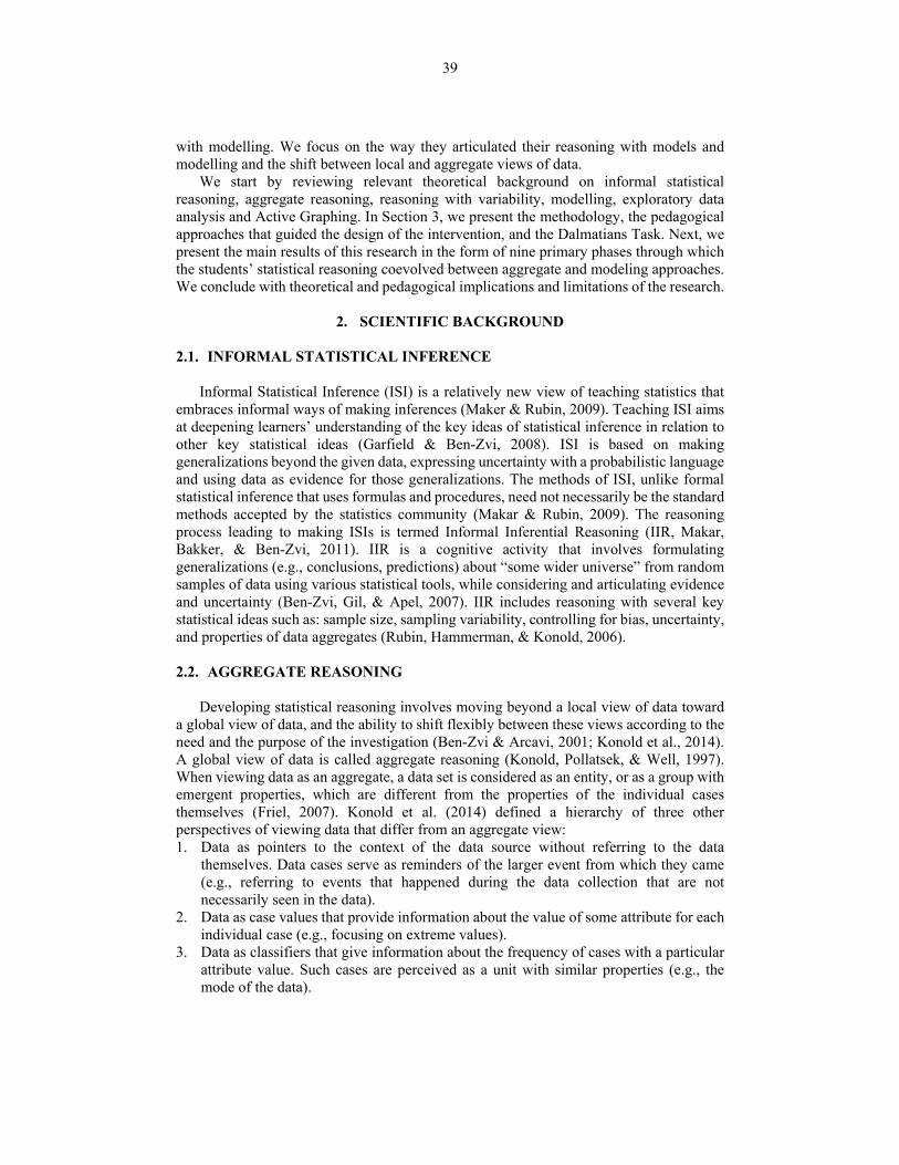
119 Iddo: Nevertheless, there are things here that are quite different: there are [leg lengths] 17 [cm, case 5] and 18 [cm, case 2]. 18 is very far from 17 [in height]. … It [this irregularity] is related also to the body structure.

The students began the realistic data investigation with a conjecture about a possible

relation (longer leg → taller) that stemmed from their contextual understanding. They viewed the data (Figure 3) mostly locally as case values (Konold et al., 2014), focusing on extreme values and comparing the variability within and between attributes, in a pointwise manner [117]. Each case supported the students’ conjecture, and this led them to change their language from conjecture to a “rule” (or a signal) [118]. Nevertheless, they were attracted by three cases—two, four and five (Figure 3)—that had the same or similar values in one attribute, but a different value in the other. They did not reject their rule, but tried to make sense of this pointwise variability, by relating it to body structure [119], a lurking attribute that was not part of the given data, rather than considering natural variability or measurement error. We therefore interpret the students’ reasoning with data at this stage as “pointwise variability explained by a lurking variable.” This search for an explanation for the noise in their data led them to the investigation described in phase 3.

Figure 3. Relation between leg length and height (case numbers added by the co-

authors)

Figure 4. Relation between tail length and

height (case numbers added by the co-authors)

Phase 3: A monotone relation and unexplained variability The students focused next

on searching for differences between or within cases by using scatter plots (such as Figure 3) and comparing the table columns and rows (Figure 1). The focus on cases four and five (in Figure 1) led the students to identify that tail length was the only attribute that distinguished between these cases, and to discover another interesting pair of cases—one and two (in Figure 1) that had the same tail length but differed in all the other attributes. They searched the data for attributes that would help them understand these irregularities and examined the relation between height and tail length (Figure 4).

246 Both: There is no relation [in the graph, Figure 4]. 250 Iddo: [But] there is a relation: The smaller the body, the shorter

the tail … This is not necessarily true, but in some cases, it [height] makes quite a difference [on tail length] … I have a fact: One part of a dog cannot be huge while the other is very small … It fits. A dog that is biggest in one attribute is relatively big in the other attributes.

48

The lack of a clear relation between height and tail length in the scatter plot (Figure 4) probably led them at first to question the suggested relation [246]. It seems that they thought relations had to be absolute—that is, they didn’t understand yet that a relation could exist and still not pertain in every case. Nevertheless, their contextual knowledge led them to generalize, “The smaller the body, the shorter the tail” [250]. Such a generalization focused on the monotonicity of the relation (see Iddo’s emphasis on claims such as, the smaller—the shorter, and “it fits”), without relating to aggregate characteristics of the relation, such as the relation’s pattern.

It seems that such articulations reflected a different view of data and its variability: While searching for a relation between two attributes, they took into account explained and unexplained variability in the data, and recognized that such relations do not always hold (“This is not necessarily true, but in some cases” [250]). This new reasoning with variability set the stage for more advanced reasoning with the data, described in phase 4.

Phase 4: Aligning signal with noise After a while, the pair returned to analysing the

relations between height and body length (Figure 5).

Figure 5. A trend line to emphasize the relation between height and body length 288 Iddo: The bigger it is here [in height]—the bigger also here [in body length], and

vice versa. 291 Yael: [Iddo is using the TinkerPlots pen to draw a trend line, Figure 5.] What Iddo

actually says is that the taller they are—the longer they are. 292 Iddo: [Drawing pairs of lines from three cases to the axes, Figure 5.] They [the

values of height and body length] are more or less the same … 296 Yael: … I think I understood how we can generate Dalmatian dogs. If, say, we

want to generate five additional dogs, we can generate one that is very tall, let’s say, with a height of 50 [cm] … It [the height] is the most related [attribute] to body length. Therefore, the difference between them [height and body length] is supposed to be very small. So its body length will be, say, 47 [cm].

The students negotiated their perceptions of the data by describing different

characteristics of data aggregation while aligning signal with noise: variability between attributes [288], covariation while considering the data as a whole [291], and a trend line to express the relation’s monotonicity as well as nature and direction (Figure 5). However, they still looked at the data locally as they drew pairs of lines from specific cases to the axes, in order to examine the similarity between the attributes’ values. These methods (trend line, and pairing values) ignited Yael’s idea how to generate more dogs. She

49

extrapolated a new case (height-50, body length-47) by adjusting height and body length taking into account what she considered so far as unexplained variability. Now it was a natural variability [296].

Phase 5: Articulations of aggregate reasoning within relations Yael invented a

method to assess the strength of a relation between two attributes (Figure 6) by making a distinction between “closed” and “open” attributes. 321 -325

Yael: I have made an inference. There are two types of distinct attributes: closed attributes and open attributes. There are the tail length and the leg length (Figure 7). These two are considered as “closed” attributes … It means that the difference between these two attributes within each dog is smaller [than other pairs of attributes]. The height and body length are also two “closed” attributes (Figure 8) … It is [the “closed” attributes are] relatively similar … If you compare it [these “closed” attributes] to leg length and body length (Figure 9), the difference between these two [leg length and tail length, Figure 7] is smaller than the difference between these two [body length and leg length, Figure 9, “open” attributes].

Figure 6. Yael’s discovery: Relations types between the attributes (translated from Hebrew, the original drawing is inside the small frame)

Figure 7. A relation between leg length and tail length: “closed” attributes

Figure 8. A relation between height and

body length: “closed” attributes

50

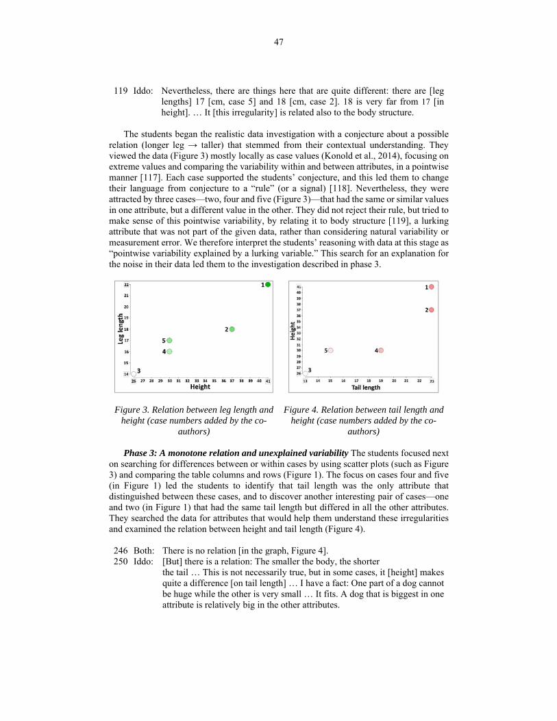
Figure 9. A relation between leg length and body length: “open” attributes The classification Yael invented for the relations between the numerical attributes in

the dogs’ population divided them into two categories: “closed” attributes that have small numeric differences between case values (e.g., height and body length) and “open” attributes which have relatively large numeric differences between case values (e.g., body length and leg length) [321]. In creating this classification, Yael accounted for measurement variability within and between relations. She reasoned in an aggregative way within relations by articulating differences between attributes and the level of their similarity (“relatively similar” [331]). It seems that the students’ continued attempts to model the dogs’ population and to take into account its irregularities encouraged them to reason with different characteristics of data aggregations and to assess attributes’ relations. These simplifications of dogs’ attributes set the ground for the construction of a TinkerPlotsTM model of the dogs’ population in the next phase.

4.2. PART II: MODELLING WORLD

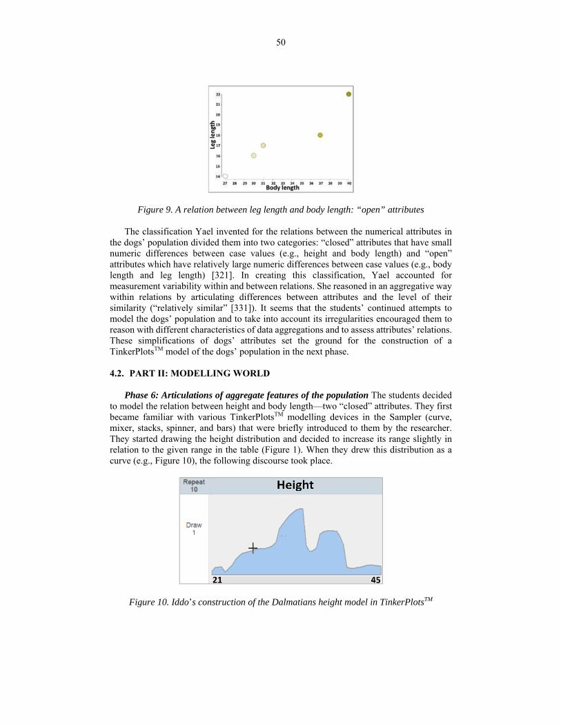
Phase 6: Articulations of aggregate features of the population The students decided

to model the relation between height and body length—two “closed” attributes. They first became familiar with various TinkerPlotsTM modelling devices in the Sampler (curve, mixer, stacks, spinner, and bars) that were briefly introduced to them by the researcher. They started drawing the height distribution and decided to increase its range slightly in relation to the given range in the table (Figure 1). When they drew this distribution as a curve (e.g., Figure 10), the following discourse took place.

Figure 10. Iddo’s construction of the Dalmatians height model in TinkerPlotsTM

51

366 Iddo: We shall first do that small [the frequency of dogs around the minimal height value of 21 cm]. There are really not many of these [near 21]. Here [near 45] …

367 Yael: There are not really many [dog’s heights] of these neither [near 45]. Most [of them] are placed in the middle. [Instructing Iddo, who holds the mouse:] Raise it [the curve] up as it gets closer to the middle, because there are not many very short dogs and also very tall dogs of this breed.

380 Yael: What I am trying to do is create different dogs’ heights, and then I shall be able to actually control it [the population], create many, many dogs’ heights, say, from 21 to 40. Then, when I see that I have all the heights [range], I try to reproduce the different heights according to the likelihood that we shall see them. The likelihood that we shall see a dog with, let’s say medium height, is higher than a really, really small or really, really tall dog. There are more chances that we shall see a dog in a height of, say 36 or 30, rather than 42.

381 Int.: How do you know that? 382 Yael: Because it [the height distribution shape] is almost like that among people

and among children. There are a few children who are really tall or really short.

In the beginning of the computer modelling process, they experimented with various

curves to create the height model. Although Iddo preferred a bimodal curve (Figure 10), Yael insisted on drawing a symmetric bell shape curve. She explained the need to set the heights according to their likelihood based on her contextual knowledge of humans [380-382].

They eventually set the dogs’ height as a discrete numeric variable using the bars device (Figure 11). Iddo drew a bumpy distribution, relating to each height’s frequency separately according to his predictions in the population (e.g., “there are not many [dogs of height] 26 [cm]” [440], “there are people who want to have only small dogs” [443]). Unlike Iddo, Yael preferred a symmetric and smooth distribution, in which heights’ frequencies were set in relation to aggregate characteristics of the population [380]. When the students ran the model to generate random samples (Figure 12), their reasoning was further extended (Phase 7).

Figure 11. The students’ final model of the Dalmatians’ height in TinkerPlotsTM

Figure 12. A random sample

generated by the height model of Figure 11

52

Phase 7: Articulations of aggregate reasoning with samples and sampling The students ran the “machine” (the Sampler) to generate random data (Figure 12) and tried to make sense of them. Yael observed that the “machine” drew values only approximately according to the model they had constructed, and scattered them throughout the height range. One particular height value (28 cm) caught her attention.

504 Yael: We gave it [the model] so many numbers. Why did it particularly choose

these numbers? And why the same number [28] twice? 505 Iddo: Because, it [the model] chose according to the percentages [Figure 11]. Do

you understand? It will not choose a number that had a low percentage. It will choose it, but less It makes a lottery, and chooses them one by one I have a feeling that if we drew a little more [a bigger sample], they will change a lot

536 Yael I noticed another thing. It [The “machine”] didn’t choose the whole interval of forties.

540 -544

Iddo We chose only ten out of, I don’t know how many, out of a million. [we need] to draw a bigger number [sample] to assure we definitely get it [a forty] There is no chance really that we shall get all these numbers. It is also a very large [range]. If we choose 10 numbers, it will surely not draw all of them here.

Based on her previous articulations [380], we assume that Yael expected the sample to

be an approximate miniature of the bell-shaped model, particularly she seemed to expect the 28 cm height to be less common than the center heights (in Figure 11). Iddo, on the other hand, took into account the relations between data, sampling variability, and randomness. He related the model frequencies to the chance of an event occurring in an unknown sized population. Such considerations led him to more sophisticated statistical reasoning with modelling by considering sample size and the sample-population relationship as important parts of reasoning about the data. Reasoning with these ideas introduced uncertainty inherent in the sampling process [540-544] and represented progress in their shared knowledge with regard to aggregate reasoning with samples and sampling. Having accepted Iddo’s explanation, the students turned to model the body length distribution (Phase 8).

Phase 8: A relation is a signal and a “controlled” variability The students added

another bar device to model the body length in the Sampler (Figure 13). They chose a similar range to the height distribution and drew an almost normal distribution shape. They generated a random sample of ten cases from their model (Figure 14), and were surprised by the absence of “order” or “a diagonal line” [Yael, 595] as in the relation they had previously recognized. They tried to change the variability in the scatter plot by editing the model. Nevertheless, changing neither the frequencies nor the ranges of the attributes helped.

After a long process of these attempts, the researcher showed the students how to design a dependency between two attributes. She explained that now they would be able “to tell the machine to set certain body lengths for which heights” [Int., 709]. The students expected that they would “need to [use] millions of devices [of the body length to model the dependency] because we want it [the model] to be precise” [Iddo, 748]. Acknowledging on their own that this method to control the variability in the data was impossible, they separated the body length to five equal intervals, and set a uniform distribution for each of them, explaining that they would change it later (Figure 15).

53

Figure 13. A TinkerPlotsTM model of the relations between Dalmatians’ height and body length

Figure 14. A random sample generated from the model of Figure 13

Figure 15. A TinkerPlotsTM model of the relation between Dalmatians’ height and body length

In the beginning of this stage, the students expected to see a clear signal of a diagonal

line in the random sample scatter plot—resembling their previous hypothesis regarding the relation between height and body length in the population. However, the absence of such a signal (Figure 14) forced them to rethink their original model (Figure 13). They believed that by changing the attributes’ range and shape they would be able to control the variability to get this signal, but were unable to find a way to do so. The new dependency tool offered them a way to control the variability better by creating “millions” of body length devices [748]. This type of reasoning however can be regarded as a regression in their aggregate reasoning with data because they wanted to create a different body length

54

distribution for each single height value, hence suggesting a type of local view of data. When the students drew a sample from their model, this perception was changed (Phase 9). Phase 9: A relation is a signal and random variability The students generated a random sample (Figure 16) from their new model (Figure 15). They were satisfied with this sample as it provided them with a “diagonal line” signal of the relation between height and body length. However, this clear signal and relative lack of noise bothered them, as “it [the model] gives us the exact same numbers” [Yael, 790]. This led Yael to describe a required refinement of their model: “dogs’ attributes values are able to shift between these things [each distribution range’s values], while keeping the rule of really a small difference between height and body length” [808]. According to Yael’s claim, the model should represent: a) a dependency relation between height and body length; b) a certain rule between these attributes; and c) a random assignment of body length values according to the defined distribution’s ranges. She therefore recommended using such refined model (Figure 15) to create the desired dog population. Nevertheless, she recognized the constraints of this model that could only roughly estimate dogs’ sizes because it was based on only seven dogs [two real and five given dogs].

Figure 16. A random sample generated by the dependency model (Figure 15)

4.3. SUMMARY OF RESULTS We summarize the results of this study in Table 3 along two dimensions: a) Yael and

Iddo’s reasoning in relation to the ways they viewed data, related to signal and noise, considered different types of variability, and articulated aggregate reasoning; and b) the pair’s reasoning with modelling, in relation to the models that they constructed during the task.

55

Table 3. Summary of the students’ articulations of aggregate and modelling reasoning

Aggregate reasoning (views of data, relating to signal and noise and types of variability)

Reasoning with modelling

Part I: Context and the data worlds Phase 1: A contextual signal based on rudimentary perspectives of variability A signal derived from the context world, based on variability, which was ordered according to certain causes.

Unexpected variability between and within dogs’ attributes raised doubts in ability to model the population.

Phase 2: Pointwise variability explained by a lurking variable Looked at data locally as case values. Compared variability between attributes among single cases. Related to variability within attributes and variability existence explained with a lurking variable.

A relation verified by looking at single cases and explaining causes of variability.

Phase 3: A monotone relation and unexplained variability Initial articulations of aggregate reasoning in relation to the relations’ monotonicity. Compared variability within and between attributes among single cases. Considered different types of variability including unexplained variability.

A signal represented by a generalization focused on the monotonicity of the relation without relating to its pattern and explained and unexplained variabilities.

Phase 4: Aligning signal with noise Expressed the signal visually as a trend line and verified it by looking at the data as case values. Related to variability within and between attributes as well as covariation while considering the data as a whole. Attempted to reason with the population aggregately, by suggesting using the signal to generate cases.

A signal within noise, described as a trend line that could be used to generate more dogs.

Phase 5: Articulations of aggregate reasoning within relations Aggregate reasoning articulations of relations. Relations between attributes defined, compared and assessed. The criterion – numeric differences between attributes’ values in cases, aggregate differences between attributes, and similarity level.

A relations classification between attributes and relations in the population that divided the attributes to two categories by numeric differences between attributes and relations.

Part II: Modelling world Phase 6: Articulations of aggregate features of the population Articulations of aggregate reasoning with the population’s height distribution, considering its range, center, shape and density, while partially connecting these statistical ideas.

Different types of models: approximately normal, bi-modal, approximately normal but bumpy distributions. Model reflected the likelihood of a height in the population.

Phase 7: Initial articulations of aggregate reasoning with samples and sampling Articulations of aggregate reasoning, relating to randomness, sampling variability, and the relations between a sample, its size, and the population. Reasoning with uncertainty about the sample.

Model reflected the chance of a height being drawn from an extreme and unknown-size population.

Phase 8: A relation is a signal and a “controlled” variability Articulations of aggregate reasoning, attending to signal and the need for a controlled variability with regard to each value in the distribution.

Model should reflect a dependency as a “diagonal line,” representing controlled variability and continuity.

Phase 9: A relation is a signal and random variability Articulations of aggregate reasoning, attending to signals within noisy processes. Expressed uncertainty regarding the data sample.

Model reflected dependency and different types of variability.

56

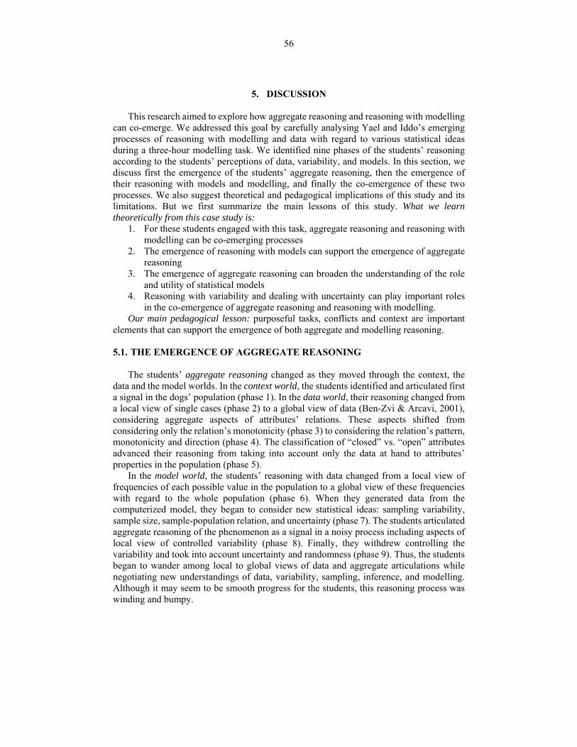
5. DISCUSSION This research aimed to explore how aggregate reasoning and reasoning with modelling

can co-emerge. We addressed this goal by carefully analysing Yael and Iddo’s emerging processes of reasoning with modelling and data with regard to various statistical ideas during a three-hour modelling task. We identified nine phases of the students’ reasoning according to the students’ perceptions of data, variability, and models. In this section, we discuss first the emergence of the students’ aggregate reasoning, then the emergence of their reasoning with models and modelling, and finally the co-emergence of these two processes. We also suggest theoretical and pedagogical implications of this study and its limitations. But we first summarize the main lessons of this study. What we learn theoretically from this case study is:

1. For these students engaged with this task, aggregate reasoning and reasoning with modelling can be co-emerging processes

2. The emergence of reasoning with models can support the emergence of aggregate reasoning

3. The emergence of aggregate reasoning can broaden the understanding of the role and utility of statistical models

4. Reasoning with variability and dealing with uncertainty can play important roles in the co-emergence of aggregate reasoning and reasoning with modelling.

Our main pedagogical lesson: purposeful tasks, conflicts and context are important elements that can support the emergence of both aggregate and modelling reasoning.

5.1. THE EMERGENCE OF AGGREGATE REASONING

The students’ aggregate reasoning changed as they moved through the context, the

data and the model worlds. In the context world, the students identified and articulated first a signal in the dogs’ population (phase 1). In the data world, their reasoning changed from a local view of single cases (phase 2) to a global view of data (Ben-Zvi & Arcavi, 2001), considering aggregate aspects of attributes’ relations. These aspects shifted from considering only the relation’s monotonicity (phase 3) to considering the relation’s pattern, monotonicity and direction (phase 4). The classification of “closed” vs. “open” attributes advanced their reasoning from taking into account only the data at hand to attributes’ properties in the population (phase 5).

In the model world, the students’ reasoning with data changed from a local view of frequencies of each possible value in the population to a global view of these frequencies with regard to the whole population (phase 6). When they generated data from the computerized model, they began to consider new statistical ideas: sampling variability, sample size, sample-population relation, and uncertainty (phase 7). The students articulated aggregate reasoning of the phenomenon as a signal in a noisy process including aspects of local view of controlled variability (phase 8). Finally, they withdrew controlling the variability and took into account uncertainty and randomness (phase 9). Thus, the students began to wander among local to global views of data and aggregate articulations while negotiating new understandings of data, variability, sampling, inference, and modelling. Although it may seem to be smooth progress for the students, this reasoning process was winding and bumpy.

57

5.2. THE EMERGENCE OF REASONING WITH MODELLING We turn now to discuss the students’ emergent reasoning with modelling. The ongoing

transitions they made between the context, data, and model worlds played a role in extending the utility of the model and in interpreting it as representative of the data. They first constructed the models in order to describe the phenomenon (phase 2), predict locally (phase 3) or globally (phases 4 and 6) possible cases in the population, and generate random data from a model (phases 7-9). Their models changed from representations that summarized only the data at hand (phase 2) to data-as-a-whole representations (phase 4) and to population representations (phases 6-9). The students’ classification of attributes in the population (phase 5) served as a bridge between the data world and the model world, as it laid the foundations for possible population models and prompted the assessment of these models.

Generating random data from the Sampler model shifted the students’ reasoning with modelling from viewing a model as static to a dynamic entity. This distinction was made by Manor Braham and Ben-Zvi (2017) and is similar to the distinction made by Konold and Pollatsek (2002) between viewing a population as static versus viewing it as a process. When a population is static, causes that might affect the population are not considered. A sample taken from a static population is viewed as a subset that allows one to make a conjecture about the whole population, even if sampling variability is considered. In contrast, when a sample or a population is viewed as a process, it is the product of an ongoing process, in which values of cases are determined by known and unknown causes (Konold & Pollatsek, 2002).

We suggest that students’ views of the population are key factors that distinguish between static and dynamic models. A model is static when it describes or predicts a population that is perceived as static. Similarly, a model is dynamic, when it represents the sample or the population as a process. In this case study, models that were discussed before the computer data generation characterized the dogs’ population as static and predictable from a sample or contextual knowledge (phase 6). After the data generation, students’ models characterized the sample or the population as processes that were influenced by known and unknown variability causes, such as the chances of events in the population, sampling variability, and randomness (phases 7-9). Thus, the students shifted from a reasoning with modelling based on context, the data at hand and variability, to a more sophisticated reasoning that took into account different types of variability and sampling as well. 5.3. THE CO-EMERGENCE OF AGGREGATE AND MODELLING

REASONING The emergence of aggregate reasoning and reasoning with modelling was guided by

the need to articulate coherent properties of the population that would mimic a real phenomenon. The search for such properties involved a repeated process of transitions between the data and the context worlds in which the students articulated, analysed, assessed, and refined possible models of these properties as well as perceptions of data. The students examined each of these conjectures in the context world in relation to their contextual knowledge about it. They then examined the conjectures in the data world to search for a noticeable structure that would justify their initial model.

In the data world, initial conjectures or models were examined locally in the data. The need to extend the inference to a wider population encouraged the students to invent methods for generalizing the identified structure in the data. With this need in mind, initial

58

articulations of aggregate reasoning emerged, as well as attempts to represent the initial models that described the population visually. The interaction in the students’ thinking about data and visual representations of generalizations advanced the students’ reasoning with data, as it emphasized the need to attend to data that agreed or disagreed with the generalization. Such considerations promoted reasoning with the relations among data, model, and the investigated phenomenon, which resulted in expansion of the model’s utility.

In the model world, the students searched for the most suitable representation that would express generalizations of the phenomenon as they constructed a model in the TinkerPlotsTM Sampler. Their shift between the Sampler’s devices gave the students an opportunity to reconsider their reasoning with data. This modelling process supported the emergence of articulations of aggregate reasoning as it involved assessing, explaining, combining, and structuring properties of the data as a whole (e.g., modelling distributions, phase 6).

Reasoning with the generated random samples (phase 7) expanded the students’ articulations of aggregate reasoning with sample and sampling. They acknowledged the sample at hand as one possible sample within many possible samples that could be drawn from the same population. The students reasoned with properties of such samples while considering sampling variability, sample size, randomness, and uncertainty. These processes were followed by questions about the sampling process and with an initial perception of the population as a process (Konold & Pollatsek, 2002), which resulted in a refinement of both aggregate reasoning and reasoning with modelling (phases 8 and 9).

The co-emergence of aggregate reasoning and reasoning with modelling provided opportunities for students to express and examine their evolving reasoning with data and modelling. They presented views of different levels of complexity at the same time and reasoned with both of them (e.g., a model as a trend line or as a line that connects data cases, phase 4, Figure 5). Such encounters can promote students’ reasoning (as the shift to a predictive model, phase 4) when they are required to choose the preferred method to articulate and model the data. Further research is necessary to study and better understand the co-emergence and development of these statistical reasoning processes.

5.4. THEORETICAL IMPLICATIONS

We identified two aspects that accompanied the co-emergence process of aggregate

reasoning and reasoning with modelling: 1) reasoning with various types and sources of variability; and 2) dealing with uncertainty.

Reasoning with various types and sources of variability The students’ reasoning

process began with a rudimentary view of variability in data—perceived as variability resulting from a certain cause, which set an order in the data. When the students recognized unexpected variability, they tried to find a cause for its existence, in order to control it in their model. If no explanation was found, they expressed doubts either in their ability to model the phenomenon (phase 1), or in the correctness of the suggested model (phase 2). Later, they accepted unexplained variability as one of the characteristics of the phenomenon (phase 3), and insisted on expressing it in their models (phase 9).

Dealing with uncertainty One of the functions of aggregate reasoning is to support the

understanding of the sample data at hand in a way that allows for an inference about the population from which the data were drawn. Such considerations entail accounting for uncertainty. The process of modelling often requires the construction of a model from a

59

situation with some level of uncertainty. In this case study, the students confronted and evaluated uncertainty while reasoning with data and modelling. They made efforts to reason with the uncertainty that was intrinsic to the problem at hand in relation to their contextual knowledge (phase 8 and 9).

Ongoing examination of the way the phenomenon was observed in the data, as well as how to model it, entailed the processes of reasoning with variability and dealing with uncertainty. This process necessitated a transition from a local view of single values as data analysis units toward reasoning with patterns or trends in the data and the population. A rudimentary perception of variability might encourage the students to search locally for data cases that fit the identified role. A more sophisticated reasoning with variability might encourage students to reason about possible data cases that are absent from their sample, and to construct models that represent such a population.

To sum up, this case study implies that reasoning with variability and dealing with uncertainty can play important roles in the co-emergence of reasoning with data and models. Further research is needed in order to study these roles.

5.5. PEDAGOGICAL IMPLICATIONS

This study gives an example of an engaging modelling task that played a part in

promoting both aggregate reasoning and reasoning with modelling. The analysis of the case study seems to suggest that purpose, conflicts, and context were three important elements that supported the development of both aggregate and modelling reasoning.

The task asked for the construction of a model that generated dogs as similar as possible to real dogs’ population. The students formulated a wide variety of conjectures based on their contextual knowledge and examined them with the data. Their reasoning with data aimed to identify a simplification of the population to describe some of the connections and relations among its components.

The specific request to generate a realistic population of Dalmatians encouraged the students to look at the aggregate and to construct a model that would address this request. However, this task led the students to focus on the most noticeable relation (height and body length) while putting aside other relations that might have been significant as well. It is therefore advisable to provide students with more than one purpose when dealing with a problem that has several different aspects. In the Dalmatian task, an additional request to provide information that would allow producing dogs’ accessories (apparel, beds, etc.) might encourage taking into account different aspects simultaneously in model construction, or constructing several different models aimed at different purposes.

Dealing with conflicts between contextual knowledge and data played an important role in the process of modelling as well as in the development of aggregate reasoning. This role included the encouragement of recognizing and identifying types of variability and its sources, as well as reasoning with uncertainty. Therefore, we suggest designing tasks in which conflicts might encourage students to articulate and carefully examine their reasoning relating to the given situation. In the Dalmatian task, we assume that a broader experience in EDA (including real data collection) and ISI before the designed shift to the modelling world might elicit such conflicts.

The context of the given problem also seems to have an important influence on the development of aggregate reasoning. We noticed that many of the students’ aggregate claims stemmed from the context world. In some stages, when the students argued in the context world, they demonstrated aggregate reasoning. At the same time, when arguing in the data world, mostly local arguments were given. We therefore suggest beginning by

60

engaging in reasoning about a real phenomenon in the context world before moving to reasoning in the data world, and later make connections between the two worlds.

5.6. LIMITATIONS

The two students chosen for this research were considered by their teachers to be both

able and verbal. In addition, both students were fond of dogs and found the subject of the research interesting and engaging. This choice was made in order to enable the collection and analysis of detailed data about their aggregate and modelling reasoning during a single three-hour task. Even after validating the data interpretation, the idiosyncrasy of the phenomena observed in this research of just a single task remain questioned. Giving such a task in a class setting might be much more challenging, and might not achieve identical results.

6. CONCLUSIONS This description is far from exhausting students’ complex processes of aggregate

reasoning and reasoning with modelling. Nevertheless, this case study presented a new aspect of the interrelations between aggregate reasoning and reasoning about modelling, which might provide an initial direction for further studies. It seems that this new line of research can advance our ongoing vision and efforts to understand and improve the learning of statistics.

ACKNOWLEDGEMENTS

This study was supported by the British Academy Small Research Grant Scheme

(SG112288). The views expressed in this article do not necessarily reflect the views or policy of the British Academy. We deeply thank Cliff Konold, Janet Ainley, Dave Pratt and the Cool-Connections research group who participated in data analysis sessions of this research. We are grateful for the helpful comments of the anonymous reviewers of earlier versions of this manuscript.

REFERENCES

Ainley, J., Aridor, K., Ben-Zvi, D., Manor, H., & Pratt, D. (2013). Children’s expressions

of uncertainty in statistical modelling. In J. Garfield (Ed.), Proceedings of the Eighth International Research Forum on Statistical Reasoning, Thinking, and Literacy (SRTL-8) (pp. 49-59). Minneapolis, MN: University of Minnesota.

Ainley, J., Nardi, E., & Pratt, D. (2000). The construction of meanings for trend in active graphing. The International Journal of Computers for Mathematical Learning, 5(2), 85-114.

Ainley, J., & Pratt, D. (2002) Purpose and utility in pedagogic task design. In A. Cockburn & E. Nardi (Eds.), Proceedings of the Twenty Sixth Annual Conference of the International Group for the Psychology of Mathematics Education (Vol. 2, pp. 17-24). Norwich, UK: PME.

Ainley, J., & Pratt, D. (2014). Expressions of uncertainty when variation is partially-determined. In K. Makar, B. de Sousa, & R. Gould (Eds.), Sustainability in statistics education (Proceedings of the 9th International Conference on Teaching Statistics, ICOTS9, July). Voorburg, The Netherlands: International Association for Statistical Education and International Statistical Institute. Retrieved from http://iase-web.org/icots/9/proceedings/pdfs/ICOTS9_9A1_AINLEY.pdf

61

Ainley, J., Pratt, D., & Nardi, E. (2001). Normalising: Children’s activity to construct meanings for trend. Educational Studies in Mathematics, 45(1-3), 131-146.

Arnold, P., Budgett, S., & Pfannkuch, M. (2013). Experiment-to-causation inference: The emergence of new considerations regarding uncertainty. In J. Garfield (Ed.), Proceedings of the Eighth International Research Forum on Statistical Reasoning, Thinking, and Literacy (SRTL-8) (CD). Minneapolis, MN: University of Minnesota.

Bakker, A., Biehler, R., & Konold, C. (2004). Should young students learn about boxplots? In G. Burrill & M. Camden (Eds.), Curricular development in statistics education, IASE 2004 Roundtable on Curricular Issues in Statistics Education, Lund Sweden (163-173). Voorburg, the Netherlands: International Statistics Institute.

Bakker, A., & Gravemeijer, K. P. E. (2004). Learning to reason about distributions. In D. Ben-Zvi & J. Garfield (Eds.), The challenge of developing statistical literacy, reasoning, and thinking (pp. 147–168). Dordrecht, The Netherlands: Kluwer Academic Publishers.

Bakker, A., & Hoffmann, M. (2005). Diagrammatic reasoning as the basis for developing concepts: A semiotic analysis of students’ learning about statistical distribution. Educational Studies in Mathematics, 60(3), 333-358.

Ben-Zvi, D., & Arcavi, A. (2001). Junior high school students’ construction of global views of data and data representations. Educational Studies in Mathematics, 45(1-3), 35–65.

Ben-Zvi, D., Gil, E., & Apel, N. (2007). What is hidden beyond the data? Helping young students to reason and argue about some wider universe. In D. Pratt & J. Ainley (Eds.), Reasoning about Informal Inferential Statistical Reasoning: A collection of current research studies. (Proceedings of the Fifth International Research Forum on Statistical Reasoning, Thinking, and Literacy (SRTL-5), pp. 29-35). Warwick, UK: University of Warwick.

Biehler, R. (1990). Changing conceptions of statistics: A problem area for teacher education. In A. Hawkins (Ed.), Proceedings of the International Statistical Institute Round Table Conference (pp. 20-38). Voorburg, The Netherlands: International Statistical Institute.

Cobb, P. (1999). Individual and collective mathematical development: The case of statistical data analysis. Mathematical Thinking and Learning, 1(1), 5-43.

Creswell, J. (2002). Educational research: Planning, conducting, and evaluating quantitative and qualitative research. Saddle River, NJ: Prentice Hall.

Friel, S. (2007). The research frontier: Where technology interacts with the teaching and learning of data analysis and statistics. In G. W. Blume & M. K. Heid (Eds.), Research on technology and the teaching and learning of mathematics: Cases and perspectives, 2 (pp. 279-331). Greenwich, CT: Information Age Publishing, Inc.

Garfield, J., & Ben-Zvi, D. (2008). Developing students’ statistical reasoning: Connecting research and teaching practice. Berlin: Springer.

Hancock, C., Kaput, J. J., & Goldsmith, L. T. (1992). Authentic inquiry with data: Critical barriers to classroom implementation. Educational Psychologist, 27(3), 337-364.

Konold, C., Higgins, T., & Russell, S. J., & Khalil, K. (2014). Data seen through different lenses. Educational Studies in Mathematics, 88(3), 305-325.

Konold, C., & Kazak, S. (2008). Reconnecting data and chance. Technology Innovations in Statistics Education, 2(1). Retrieved from http://escholarship.org/uc/item/38p7c94v

Konold, C., & Miller, C. (2011). TinkerPlots™ 2 [computer software]. Emeryville, CA: Key Curriculum Press. Available from http://www.tinkerplots.com/

Konold, C., & Pollatsek, A. (2002). Data analysis as the search for signals in noisy processes. Journal for Research in Mathematics Education, 33(4), 259-289.

62

Konold, C., Pollatsek, A., & Well, A. D. (1997). Students analyzing data: Research of critical barriers. In J. Garfield & G. Burrill (Eds.), Research on the role of technology in teaching and learning statistics (pp. 151-167). Voorburg, the Netherlands: International Statistical Institute.

Lehrer, R., Kim, M-J., Ayers, E., & Wilson, M. (2014). Toward establishing a learning progression to support the development of statistical reasoning. In J. Confrey & A. Maloney (Eds.), Learning over time: Learning trajectories in mathematics education (pp. 31-60). Charlotte, NC: Information Age Publishers.

Lehrer, R., & Schauble, L. (2000). Modelling in mathematics and science. In R. Glaser (Ed.), Advances in instructional psychology (Vol. 5, pp. 101-159). Mahwah, NJ: Lawrence Erlbaum Associates.

Lehrer, R., & Schauble, L. (2004). Modelling natural variation through distribution. American Educational Research Journal, 41(3), 635–679.

Lehrer, R., & Schauble, L. (2010). What kind of explanation is a model? In M. K. Stein (Ed.), Instructional explanations in the disciplines (pp. 9-22). New York: Springer.

Lehrer, R., & Schauble, L., (2012). Seeding evolutionary thinking by engaging children in modeling its foundations. Science Education, 96(4), 701-724.

Lehrer, R., & Schauble, L. (2015). The development of scientific thinking. In L. S. Liben & U. Müller (Vol. Eds.), R. M. Lerner (Series Ed.), Handbook of child psychology and developmental science, Vol. 2: Cognitive processes (7th ed., pp. 671-714). Hoboken, NJ: Wiley.

Lesh, R., Carmona, G., & Post, T. (2002). Models and modelling. In D. Mewborn, P. Sztajn, D. White, H. Wiegel, R. Bryant, et al. (Eds.), Proceedings of the 24th annual meeting of the North American Chapter of the International Group for the Psychology of Mathematics Education (Vol. 1, pp. 89-98) Columbus, OH: ERIC Clearinghouse.

Lesh, R., & Harel, G. (2003). Problem solving, modelling, and local conceptual development. Mathematical Thinking and Learning, 5(2), 157-189.

Makar, K., Bakker, A., & Ben-Zvi, D. (2011). The reasoning behind informal statistical inference. Mathematical Thinking and Learning, 13(1), 152-173.

Makar, K., & Rubin, A. (2009). A framework for thinking about informal statistical inference. Statistics Education Research Journal, 8(1), 82–105. Retrieved from http://iase-web.org/documents/SERJ/SERJ8(1)_Makar_Rubin.pdf

Manor Braham, H., & Ben-Zvi, D. (2017). Students’ emergent articulations of statistical models and modeling in making informal statistical inferences. Statistics Education Research Journal.

Manor Braham, H., Ben-Zvi, D., & Aridor, K. (2013). Students’ emergent reasoning about uncertainty while building informal confidence intervals in an “integrated approach.” In J. Garfield (Ed.), Proceedings of the Eighth International Research Forum on Statistical Reasoning, Thinking, and Literacy (SRTL-8) (pp. 18–33). Minneapolis, MN: University of Minnesota.

Moore, D. S. (1990). Uncertainty. In L. A. Steen (Ed.), On the shoulders of giants: A new approach to numeracy (pp. 95-137). Washington, DC: National Academy of Sciences.

Moore, D. S. (1997). New pedagogy and new content: The case of statistics. International Statistical Review, 65(2), 123-165.

Pfannkuch, M., Rubick, A., & Yoon, C. (2002). Statistical thinking: An exploration into students’ variation-type thinking. New England Mathematics Journal, 34(2), 82-98.

Pfannkuch, M., & Wild, C. (2004). Towards an understanding of statistical thinking. In D. Ben-Zvi, & J. Garfield, (Eds.), The challenge of developing statistical literacy, reasoning, and thinking (pp. 17-46). Dordrecht, The Netherlands: Kluwer Academic Publishers.

63

Reading, C., & Shaughnessy, C. (2004). Reasoning about variation. In D. Ben-Zvi, & J. Garfield (Eds.), The challenge of developing statistical literacy, reasoning and thinking (pp. 201-226). Dordrecht, The Netherlands: Kluwer Academic Publishers.

Rubin, A., Hammerman, J. K. L., & Konold, C. (2006). Exploring informal inference with interactive visualization software. In A. Rossman & B. Chance (Eds.), Working cooperatively in statistics education (Proceedings of the 7th International Conference on the Teaching of Statistics, Salvador, Bahia, Brazil, July 2-7). Voorburg, The Netherlands: International Association for Statistical Education and the International Statistical Institute. Retrieved from http://iase-web.org/documents/papers/icots7/2D3_RUBI.pdf

Schoenfeld, A. H. (2007). Method. In F. Lester (Ed.), Second handbook of research on mathematics teaching and learning (pp. 69-107). Charlotte, NC: Information Age Publishing.

Schwartz, C., & White, B. (2005). Meta-modelling knowledge: Developing students’ understanding of scientific modelling. Cognition and Instruction, 23(2), 165-205.

Siegler, R. S. (2006). Microgenetic analyses of learning. In W. Damon & R. M. Lerner (Series Eds.) & D. Kuhn & R. S. Siegler (Vol. Eds.), Handbook of child psychology: Volume 2: Cognition, perception, and language (6th ed., pp. 464–510). Hoboken, NJ: Wiley.

Tukey, J. (1977). Exploratory data analysis. Reading, MA: Addison-Wesley. Wild, C. J., & Pfannkuch, M. (1999). Statistical thinking in empirical enquiry (with

discussion). International Statistical Review, 67(3), 223-248.

KEREN ARIDOR keren.aridor@gmail.com

Faculty of Education University of Haifa

199 Aba Khoushy Ave. Mount Carmel Haifa 3498838

ISRAEL