the bootstrap method kirk wolter

P1: OTE/SPH P2: OTE

SVNY318-Wolter November 30, 2006 21:13

CHAPTER 5

The Bootstrap Method

5.1. Introduction

In the foregoing chapters, we discussed three replication-based methods of varianceestimation. Here we close our coverage of replication methods with a presenta-tion of Efron’s (1979) bootstrap method, which has sparked a massive amountand variety of research in the past quarter century. For example, see Bickel andFreedman (1984), Booth, Butler, and Hall (1994), Chao and Lo (1985, 1994),Chernick (1999), Davison and Hinkley (1997), Davison, Hinkley, and Young(2003), Efron (1979, 1994), Efron and Tibshirani (1986, 1993, 1997), Gross (1980),Hinkley (1988), Kaufman (1998), Langlet, Faucher, and Lesage (2003), Li, Lynch,Shimizu, and Kaufman (2004), McCarthy and Snowden (1984), Rao, Wu, and Yue(1992), Roy and Safiquzzaman (2003), Saigo, Shao, and Sitter (2001), Shao andSitter (1996), Shao and Tu (1995), Sitter (1992a, 1992b), and the references citedby these authors.

How does the bootstrap differ from the other replication methods? In the sim-plest case, random groups are based upon replicates of size n/k; half-samplesuse replicates of size n/2; and the jackknife works with replicates of size n − 1.By comparison with these earlier methods, the bootstrap employs replicates ofpotentially any size n∗.

We begin by describing the original bootstrap method, which used n∗ = n;i.e., the bootstrap sample is of the same size as the main sample. In subsequentsections, we adapt the original method to the problem of variance estimation infinite-population sampling and we consider the use of other values of n∗ at that time.

Let Y1, . . . , Yn be a sample of iid random variables (scalar or vector) from adistribution function F . Let θ be the unknown parameter to be estimated and let θ

denote the sample-based estimator of θ . The problem is to estimate the varianceof θ in repeated sampling from F ; i.e., Var{θ}.

194

P1: OTE/SPH P2: OTE


5.1. Introduction 195

A bootstrap sample (or bootstrap replicate) is a simple random sample withreplacement (srs wr) of size n∗ selected from the main sample. In other words,the main sample is treated as a pseudopopulation for this sampling. The bootstrapobservations are denoted by Y ∗

1 , . . . , Y ∗n .

Let θ∗ denote the estimator of the same functional form as θ but applied to thebootstrap sample instead of the main sample. Then, the ideal bootstrap estimatorof Var{θ} is defined by

v1(θ ) = Var∗{θ∗},where Var∗ signifies the conditional variance, given the main sample (or pseu-dopopulation). Repeated bootstrap sampling from the main sample produces al-ternative feasible samples that could have been selected as the main sample fromF . The idea of the bootstrap method is to use the variance in repeated bootstrapsampling to estimate the variance, Var{θ}, in repeated sampling from F .

For simple problems where θ is linear, it is possible to work out a closed-formexpression for v1(θ ). In general, however, an exact expression will not be available,and it will be necessary to resort to an approximation. The three-step procedure isto:

(i) draw a large number, A, of independent bootstrap replicates from the mainsample and label the corresponding observations as Y ∗

α1, . . . , Y ∗αn , for α =

1, . . . , A;(ii) for each bootstrap replicate, compute the corresponding estimator θ∗

α of theparameter of interest; and

(iii) calculate the variance between the θ∗α values

v2

(θ) = 1

A − 1

A∑α=1

(θ∗α − ˆθ

∗)2

,

ˆθ∗ = 1

A

A∑α=1

θ∗α .

It is clear that v2 converges to v1 as A → ∞. Efron and Tibshirani (1986) reportthat A in the range of 50 to 200 is adequate in most situations. This advice originatesfrom the following theorem, which is reminiscent of Theorem 2.6.1 for the randomgroup method.

Theorem 5.1.1. Let the kurtosis in bootstrap sampling be

β∗(θ∗) =

E∗{(

θ∗ − E∗θ∗)4}

[E∗

{(θ∗ − E∗θ∗)2

}]2− 3.

Then, given A independent bootstrap replicates,

CV{se2

(θ)} =

[CV2

{se1

(θ)} + E

{β∗

(θ∗)} + 2

4A

]1/2

,

P1: OTE/SPH P2: OTE


196 5. The Bootstrap Method

where se1(θ ) = {v1(θ )}1/2 and se2

(θ) = {v2(θ )}1/2 are the estimated standard

errors.

For large A, the difference between v1 and v2 should be unimportant. Hence-forth, we shall refer to both v1 and v2 as the bootstrap estimator of the varianceof θ .

5.2. Basic Applications to the Finite Population

We now consider use of the bootstrap method in the context of sampling froma finite population. We begin with four simple sampling designs and linear es-timators, situations in which exact results are available. Later, we address morecomplicated (and realistic) survey problems. The bootstrap method can be madeto work well for the simple surveys—where textbook estimators of variance arealready available—and this good performance motivates its use in the more com-plicated survey situations, where textbook estimates of variance are not generallyavailable. We used this line of reasoning, from the simple to the complex, previ-ously in connection with the random group, balanced half-samples, and jackknifeestimators of variance.

5.2.1. Simple Random Sampling with Replacement (srs wr)

Suppose it is desired to estimate the population mean Y of a finite populationU of size N . We select n units into the sample via srs wr sampling and use thesample mean y = (1/n)

∑yi as our estimator of the parameter of interest. From

Section 1.4, the variance of this estimator (in repeated sampling from U ) and thetextbook estimator of variance are given by

Var {y} = σ 2

n,

v (y) = s2

n,

respectively, where

σ 2 = 1

N

N∑i=1

(Yi − Y

)2,

s2 = 1

n − 1

n∑i=1

(yi − y)2.

The bootstrap sample, y∗1 , . . . , y∗

n∗ , is an srs wr of size n∗ from the parent sampleof size n, and the corresponding estimator of the population mean is the samplemean y∗ = (1/n∗)

∑y∗

i .

P1: OTE/SPH P2: OTE


5.2. Basic Applications to the Finite Population 197

Consider, for example, the first selection, y∗1 . Given the parent sample, it has

expectation and variance (in repeated sampling from the parent sample) of

E∗{

y∗1

} = 1

n

n∑i

yi ,

Var∗{

y∗1

} = 1

n

n∑i

(yi − y)2 = n − 1

ns2,

where E∗ and Var∗ denote conditional moments with respect to repeated bootstrapsampling from the parent sample (or pseudopopulation). These results follow fromthe fact that P(y∗

1 = yi ) = 1n for i = 1, . . . , n. By construction, the bootstrap ob-

servations are iid, and thus we conclude that

E∗{

y∗} = E∗{

y∗1

} = y,

v1 (y) = Var∗{

y∗} = Var∗{

y1∗}

n∗

= n − 1

n

s2

n∗ .

It is apparent that the bootstrap estimator of variance is not generally equal to thetextbook estimator of variance and is not an unbiased estimator of Var{y}. Thesedesirable properties obtain if and only if n∗ = n − 1.

Theorem 5.2.1. Given srs wr sampling of size n from the finite population of sizeN, the bootstrap estimator of variance, v1(y), is an unbiased estimator of Var{y}if and only if the bootstrap sample size is exactly one less than the size of theparent sample, n∗ = n − 1. For n∗ = n, the bias of v1(y) as an estimator of theunconditional variance of y is given by

Bias{v1(y)} = −1

nVar{y}.

In large samples, the bias is unlikely to be important, while in small samples itcould be very important indeed. For example, if the sample size were n = 2 andn∗ = n, then there would be a severe downward bias of 50%. We will discussstratified sampling in Section 5.3, where such small samples within strata are quitecommon.

5.2.2. Probability Proportional to Size Samplingwith Replacement (pps wr)

A second simple situation arises when the sample is selected via pps wr samplingand it is desired to estimate the population total, Y . To implement the sample, oneuses a measure of size Xi (i = 1, . . . , N ) and n independent, random draws fromthe distribution F = U (0, 1), say rk (k = 1, . . . , n). At the k-th draw, the procedure

P1: OTE/SPH P2: OTE



selects the unique unit i for which Si−1 < rk ≤ Si , where the cumulative sums aredefined by

Si =i∑

i ′=1

p′i for i = 1, . . . , N

= 0 for i = 0

and pi = Xi/X .The standard unbiased estimator of the population total is given by

Y = 1

n

n∑k=1

yk

pk

= 1

n

n∑k=1

N∑i=1

Irk∈(Si−1,Si ]

Yi

pi

= 1

n

n∑k=1

zk,

where yk is the y-value of the unit randomly selected at the k-th draw and Irk∈(Si−1,Si ]

is the indicator variable taking the value 1 when rk ∈ (Si−1, Si ] and 0 otherwise. Letr∗

1i, . . . , r∗

n∗ be the bootstrap sample obtained from the pseudopopulation, {ri }ni=1,

via srs wr sampling. The estimator of Y from the bootstrap sample is

Y ∗ = 1

n∗

n∗∑k=1

N∑i=1

Ir∗k ∈(Si−1,Si ]

Yi

pi.

Notice that Y ∗ is the mean of n∗ iid random variables

z∗k =

N∑i=1

Ir∗k ∈(Si−1,Si ]

Yi

pi,

each with conditional expectation

E∗{z∗

1

} = 1

n

n∑k=1

zk = Y

and conditional variance

Var∗{z∗

1

} = 1

n

n∑k=1

(zk − Y

)2.

It follows that

E∗{Y ∗} = E∗

{z∗

1

} = Y

and

Var∗{Y ∗} = Var∗

{z∗

1

}n∗

=(

n − 1

n

) (1

n∗1

n − 1

n∑k=1

(zk − Y

)2

). (5.2.1)

P1: OTE/SPH P2: OTE



v1(Y ) = Var∗{Y ∗} is the bootstrap estimator of the variance of Y . It is the factorn−1

n times the textbook estimator of the variance under pps wr sampling. If we

implement a bootstrap sample size of n∗ = n − 1, then v1

(Y

)is exactly equal to

the textbook estimator and is an unbiased estimator of Var{Y }; otherwise, whenn∗ = n, v1 is biased. If n is large, the bias may be unimportant.

5.2.3. Simple Random Sampling Without Replacement (srs wor)

The bootstrap method does not easily or uniquely accommodate without replace-ment sampling designs, even in the simplest cases. In this section, we describevariations of the standard method that might be appropriate for srs wor sampling.

The parameter of interest in this work is the population mean Y . Let s denote theparent sample of size n, and let s∗ denote the bootstrap sample of size n∗. Initially,we will assume s∗ is generated by srs wr sampling from the pseudopopulation s.We will alter this assumption later on.

The sample mean y is a standard estimator of the population mean. It is easy tofind that

E∗{

y∗} = E∗{

y∗1

}= 1

n

∑i∈s

yi

= y,

Var∗{

y∗} = Var∗{

y∗1

}n∗ (5.2.2)

=

1

n

∑i∈s

(yi − y)2

n∗

= n − 1

n

s2

n∗ .

These results are not impacted by the sampling design for the main sample butonly by the design for the bootstrap sample. Thus, these properties are the sameas in Section 5.2.1.

Compare (5.2.2) to the textbook (unbiased) estimator of variance

v (y) = (1 − f )1

ns2

and to the variance of y in repeated sampling from the population

Var {y} = (1 − f )1

nS2.

We then have the following theorem.

P1: OTE/SPH P2: OTE



Theorem 5.2.2. Assume that a bootstrap sample of size n∗ is selected via srs wrsampling from the main sample s, which itself is selected via srs wor samplingfrom the population. The standard bootstrap estimator of Var{y} is given by

v1 (y) = Var∗{

y∗} = n − 1

n

s2

n∗ . (5.2.3)

In the special case n∗ = n − 1, the bootstrap estimator

v1 (y) = s2

n

is biased upwards by the absence of the finite-population correction, 1 − f . Thebias in this case is given by

Bias {v1 (y)} = E {v1 (y)} − Var {y}= f

S2

n.

It is clear from this theorem that the bias of v1 will be unimportant wheneverf is small. In what follows, we present four variations on the standard bootstrapmethod that address survey situations in which f is not small.

Correction Factor Variant. In the special case n∗ = n − 1, an unbiased estimatorof variance is given simply by

v1F (y) = (1 − f ) v1 (y) .

Rescaling Variant. Rao and Wu (1988) define the bootstrap estimator of variancein terms of the rescaled observations

y#i = y + (1 − f )

1/2

(n∗

n − 1

)1/2 (y∗

i − y).

The method mimics techniques introduced in earlier chapters of this book inSections 2.4.3, 3.5, and 4.3.3 designed to incorporate an fpc into the randomgroup, balanced half-sample, and jackknife estimators of variance. The bootstrapmean is now

y# = 1

n∗

n∗∑i=1

y#i ,

and from (5.2.3) the bootstrap estimator of the variance is

v1R {y} = Var∗{

y#}

= (1 − f )n∗

n − 1Var∗

{y∗}

= (1 − f )1

ns2.

The rescaled variant v1R is equal to the textbook (unbiased) estimator of variance.

P1: OTE/SPH P2: OTE



Two special cases are worthy of note. If the statistician chooses n∗ = n, therescaled observations are

y#i = y + (1 − f )

1/2

(n

n − 1

)1/2 (y∗

i − y),

while the choice n∗ = n − 1 gives

y#i = y + (1 − f )

1/2(y∗

i − y).

BWR Variant. The with replacement bootstrap method (or BWR), due to Mc-Carthy and Snowden (1985), tries to eliminate the bias in (5.2.2) simply by aclever choice of the bootstrap sample size. Substituting n∗ = (n − 1) / (1 − f )into (5.2.3), we find that v1BWR (y) = (1 − f ) 1

n s2, the textbook and unbiased es-timator of Var {y} given srs wor sampling.

In practice, because (n − 1) / (1 − f ) is unlikely to be an integer, one maychoose the bootstrap sample size n∗ to be n′ = [[(n − 1) / (1 − f )]], n′′ = n′ + 1,or a randomization between n′ and n′′, where [[−]] denotes the greatest integerfunction. We tend to prefer the first choice, n∗ = n′, because it gives a conservativeestimator of variance and its bias should be small enough in many circumstances.We are not enthusiastic about the third choice, even though it can give a technicallyunbiased estimator of variance. For the Monte Carlo version of this bootstrapestimator, one would incorporate an independent prerandomization between n′

and n′′ into each bootstrap replicate.BWO Variant. Gross (1980) introduced a without replacement bootstrap (or

BWO) in which the bootstrap sample is obtained by srs wor sampling. Samplingfor both the parent and the bootstrap samples now share the without replacementfeature. In its day, this variant represented a real advance in theory, yet it nowseems too cumbersome for practical implementation in most surveys.

The four-step procedure is as follows:

(i) Let k = N/n and copy each member of the parent sample k times to create a

new pseudopopulation of size N , say U s , denoting the unit values by{

y′j

}N

j=1.

Exactly k of the y′j values are equal to yi for i = 1, . . . , n.

(ii) Draw the bootstrap sample s∗ as an srs wor sample of size n∗ from U s .

(iii) Evaluate the bootstrap mean y∗ = (1/n∗)∑n∗

i=1 y∗i .

(iv) Either compute the theoretical bootstrap estimator v1BWO (y) = Var∗ {y∗} orrepeat steps i – iii a large number of times, A, and compute the Monte Carloversion

v2BWO (y) = 1

A − 1

A∑α=1

(y∗α − 1

A

A∑α′=1

y∗α

′

)2

.

Because s∗ is obtained by srs wor sampling from U s , the conditional expectationand variance of y∗ take the familiar form shown in Section 1.4. The conditional

P1: OTE/SPH P2: OTE



expectation is

E∗{

y∗} = 1

N

N∑j=1

y′j

= k

N

∑i∈s

yi

= y,

and the conditional variance is

Var∗{

y∗} = (1 − f ∗) 1

n∗1

N − 1

N∑j=1

(y′

j − 1

N

N∑j ′=1

y′j ′

)2

= (1 − f ∗) 1

n∗k

N − 1

∑i∈s

(yi − y)2 (5.2.4)

= (1 − f ∗) 1

n∗N

N − 1

k

N(n − 1) s2,

where f ∗ = n∗/N and s2 = (n − 1)−1∑

(yi − y)2.From (5.2.4) we conclude that the theoretical bootstrap estimator

v1BWO (y) = Var∗{

y∗}is not generally unbiased or equal to the textbook estimator of variance v (y). Ifn∗ = n, then

v1BWO (y) = (1 − f )1

ns2

(N

N − 1

n − 1

n

)

and the bootstrap estimator is biased by the factor C = N (n − 1) / {(N − 1) n}. Toachieve unbiasedness, one could redefine the bootstrap estimator by multiplyingthrough by C−1,

v1BWO (y) = C−1Var∗{

y∗} ,

or by working with the rescaled values

y#i = y + C

1/2(y∗

i − y).

Another difficulty that requires additional fiddling is the fact that k = N/n isnot generally an integer. One can alter the method by working with k equal to k ′ =[[N/n]] , k ′′ = k ′ + 1, or a randomization between these bracketing integer values.Following step i, this approach creates pseudopopulations of size N ′ = nk ′, N ′′ =nk ′′, or a randomization between the two. The interested reader should see Bickeland Freedman (1984) for a complete description of the randomization method.For the Monte Carlo version of this bootstrap estimator, one would incorporate anindependent prerandomization between n′ and n′′ into each bootstrap replicate.

Mirror-Match Variant. The fourth and final variation on the standard bootstrapmethod, introduced to accommodate a substantial sampling fraction, f , is themirror-match, due to Sitter (1992a, 1992b). The four-step procedure is as follows:

P1: OTE/SPH P2: OTE



(i) Select a subsample (or one random group) of integer size m (1 ≤ m < n) fromthe parent sample, s, via srs wor sampling.

(ii) Repeat step i k times,

k = n

m

1 − e

1 − f,

independently replacing the random groups each time, where e = 1 − m/n.The bootstrap sample is the consolidation of the selected random groups andis of size n∗ = mk.

(iii) Evaluate the bootstrap mean y∗ = (1/n∗)∑n∗

i=1 y∗i .

(iv) Either compute the theoretical bootstrap estimator v1MM (y) = Var∗ {y∗}, orrepeat steps i – iii a large number of times, A, and compute the Monte Carloversion

v2MM (y) = 1

A − 1

A∑α=1

(y∗α − 1

A

A∑α′=1

y∗α′

)2

.

The bootstrap sample size,

n∗ = n1 − e

1 − f,

differs from the parent sample size by the ratio of two finite-population correctionfactors. Choosing m = f n implies the subsampling fraction e is the same as themain sampling fraction f . In this event, n∗ = n.

Let y∗j be the sample mean of the j-th selected random group, j = 1, . . . , m.

By construction, these sample means are iid random variables with conditionalexpectation

E∗{

y∗j

} = y

and conditional variance

Var∗{

y∗j

} = (1 − e)1

ms2,

s2 = 1

n − 1

n∑i=1

(yi − y)2.

It follows that the bootstrap estimator of variance is

v1MM (y) =Var∗

{y∗

j

}k

= m

n

1 − f

1 − e(1 − e)

1

ms2

= (1 − f )1

ns2,

which is the textbook and unbiased estimator of the variance Var {y}.

P1: OTE/SPH P2: OTE



A practical problem, also encountered for other variants in this section, is that kis probably not an integer. To address this problem, one could redefine k to equal

k ′ =[[

n

m

1 − e

1 − f

]],

k ′′ = k ′ + 1,or a randomization between k ′ and k ′′. The former choice gives aconservative estimator of variance. The latter choice potentially gives an unbiasedestimator provided the prerandomization between k ′ and k ′′ is incorporated in thestatement of unbiasedness. Again, for the Monte Carlo version of this bootstrapestimator, one would include an independent prerandomization into each bootstrapreplicate.

5.2.4. Probability Proportional to Size SamplingWithout Replacement (pps wor)

The last of the basic sampling designs that we will cover in this section is πpssampling, or pps wor sampling when the inclusion probabilities are proportionalto the measures of size. If Xi is the measure of size for the i-th unit, then thefirst-order inclusion probability for a sample of fixed size n is

πi = npi = Xi (X/n)−1 ;

we denote the second-order inclusion probabilities byπi j , which will be determinedby the specific πps sampling algorithm chosen. Brewer and Hanif (1983) give anextensive analysis of πps designs.

We will work in terms of estimating the population total Y . The standardHorvitz–Thompson estimator is

Y =∑i∈s

yi

πi=

∑i∈s

wi yi =1

n

∑i∈s

ui ,

where the base weight wi is the reciprocal of the inclusion probability and ui =nwi yi . Our goal is to estimate the variance of Y using a bootstrap procedure. Thetextbook (Yates–Grundy) estimator of Var

{Y

}, from Section 1.4, is

v(Y

) =n∑

i=1

n∑j>i

πiπ j − πi j

πi j

(yi

πi− y j

π j

)2

.

Unfortunately, the bootstrap method runs into great difficulty dealing with πpssampling designs. Indeed, we know of no bootstrap variant that results in a fullyunbiased estimator of variance for general n. To make progress, we will resort toa well-known approximation, namely to treat the sample as if it had been selectedby pps wr sampling. Towards this end, we let u∗

1, . . . , u∗n∗ be the bootstrap sample

P1: OTE/SPH P2: OTE



obtained by srs wr sampling from the parent sample s. The bootstrap copy of Y isthen

Y ∗ = 1

n∗

n∗∑i=1

u∗i ,

where

u∗i = (nwi yi )

∗ ,

and the u∗i random variables are iid with

E∗{u∗

1

} = 1

n

n∑i=1

ui = Y ,

Var∗{u∗

1

} = 1

n

n∑i=1

(ui − Y

)2.

The definition of u∗i is meant to imply that wi is the weight associated with yi in

the parent sample, and the pairing (wi , yi ) is preserved in specifying the bootstrapsample.

We find that

Var∗{Y ∗} = n

n∗

n∑i=1

(wi yi − 1

nY

)2

. (5.2.5)

This result follows because the conditional variance depends only on the bootstrapsampling design, not on the parent sampling design.

We designate this conditional variance as the bootstrap estimator of variance,v1

(Y

), for the πps sampling design. The choice n∗ = n − 1 gives

v1

(Y

) = n

n − 1

∑i∈s

(wi yi − 1

nY

)2

(5.2.6)

= 1

n − 1

n∑i=1

n∑j>i

(yi

πi− y j

π j

)2

,

which is the textbook and unbiased estimator of variance given pps wr sampling.By Theorem 2.4.6, we find that v1

(Y

)is a biased estimator of the variance in

πps sampling and when n∗ = n − 1 that

Bias{v1

(Y

)} = n

n − 1

[Var

{Ywr

} − Var{Y

}],

where Var{Ywr

}is the variance of the estimated total given pps wr sampling. Thus,

the bootstrap method tends to overestimate the variance in πps sampling wheneverthat variance is smaller than the variance in pps wr sampling. The bias is likely tobe small whenever n and N are both large unless the πps sampling method takesextreme steps to emphasize the selection of certain pairs of sampling units.

In small samples, the overestimation is aggravated by the factor n/ (n − 1) ≥ 1.To control the overestimation of variance when n = 2, rescaling is a possibility.

P1: OTE/SPH P2: OTE



Let n∗ = n − 1 and define the rescaled value

u#i = Y +

(π1π2 − π12

π12

)1/2 (u∗

i − Y).

The revised bootstrap estimator is

Y # = 1

n∗

n∗∑i

u#i ,

and the revised bootstrap estimator of variance is

v1R

(Y

) = Var∗{Y #

}= π1π2 − π12

π12

Var∗{Y ∗} (5.2.7)

= π1π2 − π12

π12

(w1 y1 − w2 y2)2 .

This estimator of Var{Y

}is identical to the textbook (or Yates–Grundy) estimator

of variance. Thus, the bias in variance estimation has been eliminated in this specialcase of n = 2. This method could be helpful for two-per-stratum sampling designs.Unfortunately, it is not obvious how to extend the rescaling variant to general n.Rescaling only works, however, when π1π2 > π12; that is, when the Yates–Grundyestimator is positive.

Alternatively, for general n, one could try to correct approximately for the biasin bootstrap variance estimation by introducing a correction factor variant of theform

v1F

(Y

) = (1 − f

)Var∗

{Y ∗}

= (1 − f

) n

n − 1

∑i∈s

(wi yi − 1

nY

)2

,

where n∗ = n − 1 and f = (1/n)∑n

i πi .(1 − f

)is an approximate finite-

population correction factor. While there is no universally accepted theory forthis correction in the context of πps sampling, it offers a simple rule of thumbfor reducing the overestimation of variance created by virtue of the fact thatthe uncorrected bootstrap method acts as if the sample were selected by pps wrsampling.

Throughout this section, we have based our bootstrap method on the premisethat the variance in πps sampling can be estimated by treating the sample as ifit had been obtained by pps wr sampling. Alternative approaches may be fea-sible. For example, Sitter (1992a) describes a BWO-like procedure for varianceestimation for the Rao, Hartley, and Cochran (1962) sampling design. Generally,BWO applications seem too cumbersome for most real applications to large-scale,complex surveys. Kaufman (1998) also describes a bootstrap procedure for ppssampling.

P1: OTE/SPH P2: OTE


5.3. Usage in Stratified Sampling 207

5.3. Usage in Stratified Sampling

The extension of the bootstrap method to stratified sampling designs is relativelystraightforward. The guiding principle to keep in mind in using the method is thatthe bootstrap replicate should itself be a stratified sample selected from the parentsample. In this section, we sketch how the method applies in the cases of srs wr,srs wor, pps wr, and πps sampling within strata. Details about the application tothese sampling designs have already been presented in Section 5.2.

We shall assume the population has been divided into L strata, where Nh de-notes the number of units in the population in the h-th stratum for h = 1, . . . , L .Sampling is carried out independently in the various strata, and nh denotes thesample size in the h-th stratum. The sample observations in the h-th stratum areyhi for i = 1, . . . , nh .

The bootstrap sample is y∗hi , for i = 1, . . . , n∗

h and h = 1, . . . , L . Throughoutthis section, to keep the presentation simple, we take nh ≥ 2 and n∗

h = nh − 1in all of the strata. The bootstrap replicates are one unit smaller in size than theparent sample. The detailed procedures set forth in Section 5.2 should enable theinterested reader to extend the methods to general n∗

h . We also assume throughoutthis section that the bootstrap replicate is obtained by srs wr sampling from theparent sample independently within each stratum. While BWO- and MM-likeextensions are possible, we do not present them here.

For either srs wr or srs wor sampling, the standard estimator of the populationtotal is

Y =L∑

h=1

Yh,

Yh = (Nh/nh)nh∑

i=1

yhi ,

and its bootstrap copy is

Y ∗ =L∑

h=1

Y ∗h ,

Y ∗h = (

Nh/n∗h

) n∗h∑

i=1

yhi .

The bootstrap estimator of Var{Y

}is given by

v1

(Y

) = Var∗{Y ∗} =

L∑h

Var∗{Y ∗

h

}.

The terms on the right-hand side of this expression are determined in Section 5.2.By (5.2.3), we find that

v1

(Y

) =L∑

h=1

N 2h

s2h

nh, (5.3.1)

s2h = 1

nh − 1

nh∑i

(yhi − yh)2,

P1: OTE/SPH P2: OTE



which is the textbook estimator of variance given srs wr sampling. v1 is an unbiasedestimator of variance for srs wr sampling.

On the other hand, (5.3.1) is a biased estimator of variance for srs wor samplingbecause it omits the finite-population correction factors. If the sampling fractions,fh = nh/Nh , are negligible in all of the strata, the bias should be small andv1 shouldbe good enough. Otherwise, some effort to mitigate the bias is probably desirable.The correction factor variant is not feasible here unless the sample size has been al-located proportionally to strata, in which case (1 − fh) = (1 − f ) for all strata and

v1F

(Y

) = (1 − f ) Var∗(Y ∗)

becomes the textbook (unbiased) estimator of variance. The rescaling variant isa feasible means of reducing the bias. Define the revised bootstrap observations

y#hi = yh + (1 − fh)

1/2(y∗

hi − yh),

the bootstrap copy

Y # =L∑

h=1

Y #h ,

Y #h = (

Nh/n∗h

) n∗h∑i

y#hi ,

and the corresponding bootstrap estimator of variance

v1R

(Y

) = Var∗(Y #

).

It is easy to see that v1R reproduces the textbook (unbiased) estimator of variancefor srs wor sampling:

v1R

(Y

) =L∑

h=1

N 2h (1 − fh)

s2h

nh.

For pps wr sampling, the standard estimator of the population total is

Y =L∑

h=1

Yh,

Yh = 1

nh

nh∑i=1

zhi ,

zhi = yhi

phi,


Y ∗ =L∑

h=1

Y ∗h ,

Y ∗h = 1

n∗h

n∗h∑

i=1

z∗hi ,

z∗hi =

(yhi

phi

)∗.

P1: OTE/SPH P2: OTE


5.3. Usage in Stratified Sampling 209

The bootstrap estimator of variance is given by

v1

(Y

) = Var∗{Y ∗} =

L∑h=1

Var∗{Y ∗

h

}.

By (5.2.1), we find that

v1

(Y

) =L∑

h=1

1

nh (nh − 1)

nh∑i=1

(zhi − Yh

)2,

which is the textbook (unbiased) estimator of variance.Finally, for πps sampling, the Horvitz–Thompson estimator is

Y =L∑

h=1

Yh,

Yh = 1

nh

nh∑i=1

uhi ,

uhi = nhwhi yhi ,

whi = 1

πhi,


Y ∗ =L∑

h=1

Y ∗h ,

Y ∗h = 1

n∗h

n∗h∑

i=1

u∗hi ,

u∗hi = (nhwhi yhi )

∗.

Given the approximation of treating the sample as if it were a pps wr sample, thebootstrap estimator of variance is (from 5.2.6)

v1

(Y

) = Var∗{Y ∗}

=L∑

h=1

Var∗{Y ∗

h

}(5.3.2)

=L∑

h=1

nh

nh − 1

nh∑i=1

(whi yhi − 1

nhYh

)2

.

For πps sampling, (5.3.2) is biased and, in fact, overestimates Var{Y

}to the extent

that the true variance given πps sampling is smaller than the true variance givenpps wr sampling.

P1: OTE/SPH P2: OTE



Two-per-stratum sampling designs are used in certain applications in whichnh = 2 for h = 1, . . . , L . The bias in variance estimation can be eliminated byworking with the rescaled observations

u#hi = Yh +

(πh1πh2 − πh12

πh12

)1/2 (u∗

hi − Yh)

and the revised bootstrap copy

Y # =L∑

h=1

Y #h ,

Y #h = 1

n∗h

n∗h∑

i=1

u#hi .

5.4. Usage in Multistage Sampling

In this section, we shall address survey designs with two or more stages ofsampling and with pps sampling either with or without replacement at the firststage. We shall continue to focus on the estimation of the population total,Y .

Consider an estimator of the form

Y =L∑h

Yh,

Yh = 1

nh

nh∑i

Yhi

phi= 1

nh

nh∑i

zhi ,

zhi = Yhi/phi .

In this notation, there are L strata, and nh PSUs are selected from the h-thstratum via pps wr sampling according to the per-draw selection probabilities(i.e.,

∑nhi phi = 1

). Sampling is assumed to be independent from stratum to stra-

tum. Yhi is an estimator of Yhi , the total within the i-th PSU in the h-th stratum, dueto sampling at the second and successive stages of the sampling design. We are notespecially concerned about the form of Yhi —it could be linear in the observations,a ratio estimator of some kind, or something else. Of course, Yhi should be goodfor estimating Yhi , which implies that it should be unbiased or approximately so.However, the estimators of variance that follow do not require unbiasedness. Inpractical terms, the same estimator (the same functional form) should be used foreach PSU within a stratum.

P1: OTE/SPH P2: OTE


5.4. Usage in Multistage Sampling 211

To begin, assume pps wr sampling, where it is well-known that an unbiasedestimator of the unconditional variance, Var

{Y

}, is given by

v(Y

) =L∑h

v(Yh

)

=L∑h

1

nh (nh − 1)

nh∑i

(zhi − Yh

)2. (5.4.1)

We obtain the bootstrap sample by the following procedure:

(i) Select a sample of n∗1 PSUs from the parent sample (pseudopopulation) in the

first stratum via srs wr sampling.(ii) Independently, select a sample of n∗

2 PSUs from the parent sample in thesecond stratum via srs wr sampling.

(iii) Repeat step ii independently for each of the remaining strata, h = 3, . . . , L .(iv) Apply the ultimate cluster principle, as set forth in Section 2.4.1. This means

that when a given PSU is taken into the bootstrap replicate, all second andsuccessive stage units are taken into the replicate also. The bootstrap replicateis itself a stratified, multistage sample from the population. Its design is thesame as that of the parent sample.

The bootstrap sample now consists of the z∗hi for i = 1, . . . , n∗

h and h =1, . . . , L .

The observations within a given stratum, h, have a common expectation andvariance in bootstrap sampling given by

E∗{z∗

hi

} = 1

nh

nh∑i

zhi = Yh,

Var∗{z∗

hi

} = 1

nh

nh∑i

(zhi − Yh

)2.

Therefore, we find the following theorem.

Theorem 5.4.1. The ideal bootstrap estimator of variance is given by

v1

(Y

) =L∑h

Var∗{Y ∗

h

}

=L∑h

Var∗{z∗

h1

}n∗

h

(5.4.2)

=L∑h

1

n∗h

1

nh

nh∑i

(zhi − Yh

)2.

The estimator (5.4.2) equals the textbook (unbiased) estimator (5.4.1) when n∗h =

nh − 1.

P1: OTE/SPH P2: OTE



For other values of the bootstrap sample size, such as n∗h = nh , v1 is a biased

estimator of the unconditional variance Var{Y

}. The bias may be substantial for

small nh , such as for two-per-stratum designs.Next, let us shift attention to multistage designs in which a πps application is

used at the first stage of sampling. The estimator of the population total is nowdenoted by

Y =L∑

h=1

Yh

=L∑

h=1

nh∑i=1

∑j∈shi

whij yhij

=L∑

h=1

1

nh

nh∑i=1

uhi.,

uhi j = nhwhij yhij,

uhi. =∑j∈shi

uhij,

where whi j is the survey weight attached to the (h, i, j)-th ultimate sampling unit(USU) and shi is the observed set of USUs obtained as a result of sampling at thesecond and successive stages within the (h, i)-th PSU.

Although we have shifted to without replacement sampling at the first stage, weshall continue to specify the bootstrap sample as if we had used with replacementsampling. We employ the five-step procedure that follows (5.4.1). The bootstrapsample consists of

u∗hi. =

(∑j∈shi

nhwhij yhij

)∗

for i = 1, . . . , n∗h and h = 1, . . . , L . This notation is intended to convey the ulti-

mate cluster principle, namely that selection of the PSU into the bootstrap replicatebrings with it all associated second and successive stage units.

The bootstrap copy of Y is given by

Y ∗ =L∑

h=1

Y ∗h =

L∑h=1

1

n∗h

n∗h∑

i=1

u∗hi. (5.4.3)

=L∑

h=1

nh∑i=1

∑j∈shi

wαhi j yhij,

where the bootstrap weights are given by

wαhij = tαhinh

n∗h

whij (5.4.4)

and tαhi is the number of times the (h, i)-th PSU in the parent sample is selected intothe bootstrap replicate,α. The valid values are tαhi = 0, 1, . . . , n∗

hi .For nonselected

P1: OTE/SPH P2: OTE


5.4. Usage in Multistage Sampling 213

PSUs (into the bootstrap sample), tαhi = 0 and the corresponding bootstrap weightsare null, wαhi j = 0. For selected but nonduplicated PSUs (in the bootstrap sample),tαhi = 1 and the bootstrap weights

wαhij = nh

n∗h

whij

reflect the product of the original weight in the parent sample and the reciprocal ofthe bootstrap sampling fraction. For selected but duplicated PSUs (in the bootstrapsample), tαhi ≥ 2 and the bootstrap weights reflect the product of the originalweight, the reciprocal of the bootstrap sampling fraction, and the number of timesthe PSU was selected.

The ideal bootstrap estimator of variance is now

v1

(Y

) = Var∗{Y ∗} =

L∑h=1

Var∗{Y ∗

h

}

=L∑

h=1

Var∗{u∗

h1.

}n∗

h

(5.4.5)

=L∑

h=1

1

n∗h

1

nh

nh∑i=1

(uhi. − Yh

)2

=L∑

h=1

nh

n∗h

nh∑i=1

⎛⎝∑

j∈shi

whi j yhij − 1

nhYh

⎞⎠

2

.

Its properties are set forth in the following theorem.

Theorem 5.4.2. Given πps sampling, the ideal bootstrap estimator of the varianceVar

{Y

}, given by (5.4.5), is equivalent to the random group estimator of variance

(groups of size 1 PSU) if and only if nh ≥ 2 and n∗h = nh − 1. In addition to these

conditions, assume that the survey weights are constructed such that

Yhi.

πhi= E

⎧⎨⎩

∑j∈shi

whij yhij|i⎫⎬⎭ ,

σ 22hi

π2hi

= Var

⎧⎨⎩

∑j∈shi

whij yhij|i⎫⎬⎭ ,

and

0 = Cov

⎧⎨⎩

∑j∈shi

whij yhij,∑

j ′∈sh′ i ′

wh′i ′ j ′ yh′i ′ j ′ |i, i ′

⎫⎬⎭

for (h, i) = (h′, i ′), where Yhi. is the population total within the (h, i)-th selected

PSU and πhi is the known probability of selecting the (h, i)-th PSU. The variance

P1: OTE/SPH P2: OTE



component σ 22hi is due to sampling at the second and successive stages. Then, the

unconditional expectation of the bootstrap estimator is

E{v1

(Y

)} =L∑

h=1

⎡⎣E

⎧⎨⎩ nh

nh−1

nh∑i=1

(Yhi.

πhi− 1

nh

nh∑i ′=1

Yhi ′.

πhi ′

)2⎫⎬⎭ +

Nh∑i=1

σ 22hi

πhi

⎤⎦.

(5.4.6)

Because the unconditional variance of Y is given by

Var{Y

} =L∑

h=1

[Var

{nh∑

i=1

Yhi.

πhi

}+

Nh∑i=1

σ 22hi

πhi

], (5.4.7)

we conclude that the bootstrap estimator correctly includes the within PSU com-ponent of variance, reaching a similar finding as for the random group estimatorin (2.4.10). The bias in the bootstrap estimator—the difference between the firstterms on the right-hand sides of (5.4.6) and (5.4.7)—arises only in the betweenPSU component of variance. Furthermore, we conclude from Theorem 2.4.6 thatthe bias in the bootstrap estimator is

Bias{v1

(Y

)} =L∑

h=1

nh

nh − 1

(Varwr

{1

nh

nh∑i=1

Yhi.

phi

}− Varπps

{nh∑

i=1

Yhi.

πhi

}),

where Varwr means the variance in pps wr sampling and Varπps means the variancein πps sampling. The bootstrap estimator is upward biased whenever πps samplingis superior to pps wr sampling.

For nh = 2, one could consider using the rescaling technique to adjust the boot-strap estimator of variance to eliminate the bias in the between PSU componentof variance. However, this effort may ultimately be considered unacceptable be-cause it would introduce bias into the estimation of the within PSU component ofvariance.

5.5. Nonlinear Estimators

We now consider bootstrap variance estimation for nonlinear estimators. A generalparameter of the finite population is

θ = g (T) ,

where g is continuously differentiable and T is a p × 1 vector of population totals.For a general probability sampling plan giving a sample s, let T be the textbook(unbiased) estimator of T. The survey estimator of the general parameter is θ =g(T).

The bootstrap method for this problem consists of eight broad steps:

(i) Obtain a bootstrap replicate s∗1 by the methods set forth in Sections 5.2–5.4.

P1: OTE/SPH P2: OTE


5.5. Nonlinear Estimators 215

(ii) Let T∗1 be the bootstrap copy of the estimated totals based upon the bootstrap

replicate.(iii) Compute the bootstrap copy of the survey estimator θ∗

1 = g(T∗1).

(iv) Interest centers on estimating the unconditional variance Var{θ}. If feasible,

compute the ideal bootstrap estimator of variance as v1

(θ) = Var∗

{θ∗

1

}and

terminate the bootstrap estimation procedure. Otherwise, if a known, closed-form expression does not exist for the conditional variance Var∗

{θ∗

1

}, then

continue to the next steps and use the Monte Carlo method to approximatethe ideal bootstrap estimator.

(v) Draw A − 1 more bootstrap replicates, s∗α , giving a total of A replicates. The

replicates should be mutually independent.(vi) Let T∗

α be the bootstrap copies of the estimated totals for α = 1, . . . , A.

(vii) Compute the bootstrap copies of the survey estimator θ∗α = g(T∗

α) for α =1, . . . , A.

(viii) Finally, compute the Monte Carlo bootstrap estimator of variance

v2

(θ) = 1

A − 1

A∑α=1

(θ∗α − ˆθ

∗)2

, (5.5.1)

ˆθ∗ = 1

A

A∑α=1

θ∗α .

As a conservative alternative, one could compute v2 in terms of squared differ-

ences about θ instead of ˆθ∗.

As an example, we show how the method applies to the important problemof ratio estimation. Suppose we have interviewed a multistage sample selectedwithin L strata, obtaining measurements yhij, xhij for the j-th ultimate samplingunit (USU) selected within the i-th primary sampling unit (PSU) obtained in theh-th stratum. The textbook estimators of the population totals are

Y =L∑

h=1

nh∑i=1

mhi∑j=1

whij yhij,

X =L∑

h=1

nh∑i=1

mhi∑j=1

whijxhij,

where nh is the number of PSUs selected within stratum h, mhi is the numberof USUs interviewed within the (h, i)-th PSU, and whi j is the survey weight forthe (h, i, j)-th USU. The survey weights reflect the reciprocals of the inclusionprobabilities and perhaps other factors, and they are specified such that Y and Xare unbiased or nearly unbiased estimators of the corresponding population totalsY and X .

The ratio of the two totals θ = Y/X is often of interest in survey research.The usual survey estimator of the population ratio is the ratio of the estimatedtotals θ = Y/X . To estimate the unconditional variance of θ , obtain independent

P1: OTE/SPH P2: OTE



bootstrap replicates α = 1, . . . , A as in Section 5.4. Compute the bootstrap copies

Y ∗α =

L∑h=1

nh∑i=1

mhi∑j=1

wαhij yhij,

X∗α =

L∑h=1

nh∑i=1

mhi∑j=1

wαhijxhij,

where the replicate weights are defined in (5.4.4). Also, compute the bootstrapcopies of the ratio θ∗

α = Y ∗α /X∗

α , α = 1, . . . , A. Finally, evaluate the bootstrapestimator of variance v2

(θ)

as in (5.5.1).Another prominent parameter of interest in survey research is defined as the

solution to the equation

N∑i=1

{Yi − μ (Xiθ )}Xi = 0.

The case of a dichotomous (0 or 1) dependent variable y and

μ (xθ ) = exθ

1 + exθ

corresponds to simple logistic regression, while a general dependent variable y andμ (xθ ) = xθ corresponds to ordinary least squares regression. Given the aforemen-tioned multistage, stratified sampling plan, the standard estimator θ is defined asthe solution to the equation

L∑h=1

nh∑i=1

mhi∑j=1

whij{

yhi j − μ(xhi jθ

)}xhi j = 0.

The estimator θ may be obtained by Newton–Raphson iterations

θ (k+1) = θ (k)

+{

L∑h=1

nh∑i=1

mhi∑j=1

whijμ′(xhi j θ

(k))x2

hi j

}−1 L∑h=1

nh∑i=1

mhi∑j=1

whij{

yhi j −μ(xhi j θ

(k))}

xhi j ,

where

μ′ (xθ ) = μ (xθ ) {1 − μ (xθ )} , if logistic regression,

= 1, if ordinary least squares regression.

Given bootstrap replicate α, the bootstrap copy of the estimator θ∗α is defined as

the solution to

L∑h=1

nh∑i=1

mhi∑j=1

wαhij {yi − μ (xiθ )} = 0,

P1: OTE/SPH P2: OTE


5.6. Usage for Double Sampling Designs 217

where the replicate weights are defined in (5.4.4). Using A bootstrap replicatesyields the bootstrap estimator of the unconditional variance of θ ,

v2

(θ) = 1

A − 1

A∑α=1

(θ∗α − ˆθ

∗)2

.

The method extends straightforwardly to the multivariate case: μ (Xiθ ), where Xi

is (1 × p) and θ is (p × 1).Before leaving this section, we briefly address a key question: Why should

one trust the bootstrap method to provide a valuable estimator of variance for anonlinear estimator θ? An informal answer to this question is that the method workswell for linear estimators, where we have demonstrated that it has the capacity toreproduce the textbook (unbiased) estimator of variance. The proper choice of n∗

and rescaling may be necessary to achieve exact unbiasedness. Since the methodworks for linear statistics, it should also work for nonlinear statistics that havea local linear quality. This justification for the bootstrap method is no differentfrom that given in earlier chapters for the random group, BHS, and jackknifemethods.

That said, little is known about the exact theoretical properties of the bootstrapestimator of variance in small samples. Appendix B.4 presents some asymptotictheory for the method and establishes conditions under which the normal approx-

imation to(θ − θ

)/

√v1

(θ)

is valid and thus in which the bootstrap can be used

with trust to construct statistical confidence intervals.

5.6. Usage for Double Sampling Designs

Double sampling designs are used to achieve various ends, such as improvedprecision of survey estimation or the oversampling of a rare population. In thissection, we demonstrate how the bootstrap method can be applied to estimate thevariance for such sampling designs. The guiding principle is similar to that set forthin Section 2.4.1, namely that the bootstrap replicate should have the same doublesampling design as the parent sample. Here we will assume srs wr sampling at eachphase of the design and that the parameter of interest is the population mean Y .The bootstrap method readily extends to other double sampling designs (includingother sampling schemes, parameters, and estimators).

Assume the following methods of sampling and estimation.

(i) Draw a sample of size n2 by srs wr sampling and collect the data (yi , xi ) forthe units in the selected sample.

(ii) Independently draw a supplementary sample of size n3 by srs wr samplingand collect the data xi for the units in this selected sample.

(iii) Construct a regression estimator of the population mean

yR = y2 + B (x1 − x2) ,

P1: OTE/SPH P2: OTE



where

y2 = 1

n2

n2∑i=1

yi ,

x2 = 1

n2

n2∑i=1

xi ,

are the sample means of the y- and x-variables for the sample specified instep i;

x3 = 1

n3

n2+n3∑i=n2+1

xi

is the sample mean of the x-variable in the supplementary sample; B is aknown constant; n1 = n2 + n3 is the size of the pooled sample; λ2 = n2/n1

and λ3 = n3/n1 are the proportions of the pooled sample; and

x1 = λ2 x2 + λ3 x3

is the mean of the pooled sample.

The premise of the double sampling scheme is that it is much more expensive tocollect data on y than on x . One can afford to collect x on a substantially largersample than the sample used to collect y. For example, collection of y may requirea personal interview with respondents, while collection of x may be based onprocessing of available administrative records.

The pooled sample n1 is called the first phase of the double sampling scheme.The sample n2 is called the second phase of the design. x is collected for allof the units in the first-phase sample, while y is collected only for units in thesecond-phase sample.

The regression estimator can be rewritten as

yR = r2 + Bλ2 x2 + Bλ3 x3,

where

ri = yi − Bxi ,

r2 = 1

n2

n2∑i=1

ri .

Because the supplementary sample is independent of the second-phase sample, itfollows that

Var {yR} = Var {r2} + B2λ22Var {x2} + 2Bλ2Cov {r2, x2} + B2λ2

3Var {x3}

= σ 2r

n2

+ B2λ22

σ 2x

n2

+ 2Bλ2

σr x

n2

+ B2λ23

σ 2x

n3

,

P1: OTE/SPH P2: OTE


5.6. Usage for Double Sampling Designs 219

where the population variances and covariances are defined by

σ 2r = 1

N

N∑i=1

(Ri − R

)2,

σ 2x = 1

N

N∑i=1

(Xi − X

)2,

σ 2r x = 1

N

N∑i=1

(Ri − R

) (Xi − X

),

Ri = Yi − Xi B.

Assuming n2 ≥ 2 and n3 ≥ 2, a standard textbook estimator (unbiased) of thevariance Var {yR} is

v (yR) = s22r

n2

+ B2λ22

s22x

n2

+ 2Bλ2

s2r x

n2

+ B2λ23

s23x

n3

,

where

s22r = 1

n2 − 1

n2∑i=1

(ri − r2)2,

s22x = 1

n2 − 1

n2∑i=1

(xi − x2)2,

s23x = 1

n3 − 1

n3∑i=1

(xi − x3)2,

s2r x = 1

n2 − 1

n2∑i=1

(ri − r2) (xi − x2)2.

The data from the double sampling design are given by (y1, x1, y2, x2, . . . ,

yn2, xn2

, xn2+1, . . . , xn1). In this notation, the observations in the supplementary

sample are indexed by i = n2 + 1, n2 + 2, . . . , n1. A bootstrap sample for thisproblem consists of a random sample from the second-phase sample and an in-dependent random sample from the supplementary sample. Thus, the bootstrapsample uses the two-phase sampling design. Here is the four-step procedure forspecifying a bootstrap sample.

(i) Draw a sample of size n∗2 from the second-phase sample n2 by srs wr sampling.

(ii) Draw an independent sample of size n∗3 from the supplementary sample n3

by srs wr sampling.(iii) The pooled bootstrap replicate, or first-phase sample, consists of the second-

phase sample and the supplementary sample and is of size n∗1 = n∗

2 + n∗3.

(iv) Construct the bootstrap copy of the regression estimator

y∗R = y∗

2 + B(x∗

1 − x∗2

)= r∗

2 + Bλ2 x∗2 + Bλ3 x∗

3 .

P1: OTE/SPH P2: OTE



Because bootstrap sampling is independent in the second-phase and supplemen-tary samples, we find the following theorem.

Theorem 5.6.1. Assuming n∗2 ≥ 2 and n∗

3 ≥ 2, the ideal bootstrap estimator ofthe unconditional variance Var {yR} is defined by

v1 (yR) = Var∗{

y∗R

}= Var∗

{r∗

2

} + B2λ22Var∗

{x∗

2

}+ 2Bλ2Cov∗

{r∗

2 , x∗2

}+ B2λ2

3Var∗{

x∗3

}= n2 − 1

n2

1

n∗2

s22r + B2λ2

2

n2 − 1

n2

1

n∗2

s22x

+ 2Bλ2

n2 − 1

n2

1

n∗2

s2r x

+ B2λ23

n3 − 1

n3

1

n∗3

s23x .

Furthermore, if n∗2 = n2 − 1 and n∗

3 = n3 − 1, this ideal bootstrap estimator re-produces the textbook (unbiased) estimator of variance.

Throughout the foregoing presentation, we assumed B is a fixed and knownconstant. Now assume B2 is an estimator based upon the second-phase sample, suchas the ordinary least squares estimator B2 = ∑

(xi − x2) (yi − y2) /∑

(xi − x)2

or the ratio B2 = y2/x2. In the latter case, the estimator of the population meanbecomes the ratio estimator

yR = y2

x2

x1.

The estimator of the population mean is now nonlinear, and a closed-form, simpleexpression for the ideal bootstrap estimator of variance does not exist. We willresort to the Monte Carlo version of the bootstrap for this problem.

A bootstrap replicate is obtained by steps i –iv above, where the bootstrap copyof yR is now given by

y∗R = y∗

2 + B∗2

(x∗

1 − x∗2

)and B∗

2 is the estimator B2 based upon the n∗2 units selected into the second phase

of the bootstrap replicate. For example, in the ratio case B∗2 = y∗

2/x∗2 and in the

ordinary least squares case, B∗2 = ∑ (

x∗i − x∗

2

) (y∗

i − y∗2

)/∑ (

x∗i − x∗

2

)2.

The complete bootstrap procedure now consists of steps i – iv plus the followingtwo additional steps:

(v) Replicate steps i–iv independently A − 1 more times.

P1: OTE/SPH P2: OTE


5.7. Example: Variance Estimation for the NLSY97 221

(vi) Compute the bootstrap copy y∗Rα for each bootstrap replicate α = 1, . . . , A.

The bootstrap estimator of the unconditional variance Var {yR} is finally givenby

v2 (yR) = 1

A − 1

A∑α=1

(y∗

Rα − y∗R.

)2,

where y∗R. equals either

∑y∗

Rα/A or yR . In practice, we can recommendn∗

2 = n2 − 1 and n∗3 = n3 − 1, as before.

5.7. Example: Variance Estimation for the NLSY97

Examples of bootstrap variance estimation for complex sample surveys are givenby Li et al. (2004), Langlet, Faucher, and Lesage (2003), and Kaufman (1998).In this final section of Chapter 5, we present an example of the bootstrap methodbased on data collected in the National Longitudinal Survey of Youth (NLSY97).This work continues the example begun in Section 4.7.

We used custom SAS programming to compute the bootstrap estimates.1 Sincewe are treating the NLSY97 as a stratified, multistage sampling design, we used themethods set forth in Section 5.4 to construct A = 200 bootstrap replicates, each ofsize n∗

h = nh − 1, for h = 1, . . . , 323. We used the methods of Section 5.5 to con-struct bootstrap variance estimates for the nonlinear ratio statistics described below.

In Section 4.7, we presented jackknife and BHS variance estimates both withand without replicate reweighting. We found that the resulting variance estimatesdiffered only trivially. Thus, in what follows, we present results of the use of theBHS, jackknife, and bootstrap methods without reweighting for nonresponse andother factors within each replicate. Replicate weights for the bootstrap method arebased solely on (5.4.4).

Table 5.7.1 shows the estimated percentage of enrolled youths (or students) whoworked during the 2000–01 school year or the summer of 2001. The weightedestimates are broken down by age (17, 18, or 19) and by age crossed by sex,race/ethnicity, or grade. These data also appear in Table 4.7.1. The table displays theestimated standard errors obtained by the BHS, jackknife, and bootstrap methods.The three standard errors are reasonably close to one another for all of the statisticsstudied in this table.

The bootstrap method offers the smallest average standard error (1.82) and yieldsthe largest standard error for 8 individual domains and the smallest standard errorfor 11 domains. By comparison, the BHS method has an average standard errorof 1.85 and is the largest standard error in four cases and the smallest in ninecases. The jackknife method has the largest average standard error (1.86) and isthe largest standard error in 13 cases and the smallest in 8 cases. Figure 5.7.1 plots

1 All of the calculations for the bootstrap method were performed by Erika Garcia-Lopezin connection with coursework in the Department of Statistics, University of Chicago.

P1: OTE/SPH P2: OTE



Table 5.7.1. Percentage of Students Who Ever Worked During the School Yearor Following Summer

Jackknife BHS BootstrapDomain Estimates Standard Error Standard Error Standard Error

Total, age 17 89.0 1.00 0.98 1.05

Male youths 88.5 1.49 1.35 1.42

Female youths 89.6 1.23 1.36 1.32

White non-Hispanic 92.2 1.04 1.09 1.16

Black non-Hispanic 78.7 3.18 2.76 2.53

Hispanic origin 86.8 2.34 2.55 2.91

Grade 11 84.8 2.63 2.63 2.61

Grade 12 90.9 1.19 1.05 1.06

Total, age 18 90.5 1.22 1.21 1.11

Male youths 89.3 2.05 1.90 1.81

Female youths 91.8 1.32 1.55 1.52




Grade 12 86.7 1.91 2.16 2.32

Freshman in college 93.9 1.27 1.34 1.36

Total, age 19 94.1 1.20 1.13 1.12

Male youths 93.8 1.61 1.64 1.66

Female youths 94.4 1.43 1.42 1.43




Freshman in college 95.2 1.91 1.89 1.92

Sophomore in college 95.1 1.42 1.43 1.48

0.0

0.5

1.0

1.5

2.0

2.5

3.0

3.5

4.0

0.0 0.5 1.0 1.5 2.0 2.5 3.0 3.5 4.0Jackknife S.E. Estimates

S.E

. E

sti

mate

s

BHS Estimates Bootstrap Estimates

Figure 5.7.1 Plot of Alternative Standard Error Estimates versus the Jackknife Standard

Error Estimates.

P1: OTE/SPH P2: OTE



Table 5.7.2. Estimates of Percentage of Students Who Ever Worked During theSchool Year or Following Summer from 200 Bootstrap Replicates: Females,Age 18

Bootstrap Bootstrap Bootstrap BootstrapReplicate Replicate Replicate ReplicateNumber Estimates Number Estimates Number Estimates Number Estimates

1 91.18 51 88.23 101 93.24 151 93.22

2 90.91 52 92.08 102 92.58 152 90.20

3 93.33 53 91.70 103 93.10 153 90.52

4 93.41 54 92.50 104 92.69 154 88.98

5 93.12 55 90.92 105 91.78 155 95.30

6 91.66 56 92.62 106 91.83 156 93.12

7 93.91 57 94.35 107 91.59 157 94.31

8 90.90 58 90.28 108 94.34 158 89.95

9 90.81 59 89.01 109 89.65 159 91.35

10 91.10 60 91.12 110 92.89 160 91.88

11 92.69 61 89.41 111 91.10 161 90.65

12 92.49 62 90.27 112 89.45 162 94.47

13 91.30 63 91.02 113 92.25 163 91.78

14 92.78 64 90.05 114 91.83 164 91.07

15 92.81 65 92.83 115 92.35 165 90.98

16 90.43 66 94.06 116 91.45 166 94.01

17 89.95 67 92.47 117 95.00 167 92.00

18 94.49 68 90.62 118 93.42 168 93.50

19 90.21 69 91.08 119 90.43 169 94.63

20 91.09 70 92.46 120 95.10 170 87.78

21 92.29 71 92.09 121 90.94 171 90.13

22 92.85 72 92.15 122 90.97 172 93.30

23 92.47 73 93.07 123 91.21 173 90.48

24 91.82 74 93.76 124 93.64 174 89.47

25 91.60 75 94.28 125 91.94 175 91.25

26 92.41 76 93.93 126 91.87 176 92.10

27 93.73 77 94.96 127 93.10 177 90.53

28 89.28 78 93.33 128 91.09 178 91.93

29 91.55 79 91.20 129 91.40 179 91.22

30 92.66 80 90.56 130 93.34 180 89.64

31 91.98 81 94.94 131 94.20 181 89.84

32 92.00 82 91.80 132 93.40 182 91.00

33 93.74 83 89.07 133 93.53 183 92.18

34 92.44 84 92.72 134 92.50 184 92.23

35 91.35 85 88.56 135 88.47 185 92.89

36 92.41 86 92.18 136 92.55 186 89.55

37 92.77 87 89.07 137 92.99 187 90.34

38 90.88 88 93.50 138 90.32 188 91.93

39 91.62 89 91.66 139 90.37 189 92.22

40 91.29 90 92.91 140 93.93 190 90.23

41 91.11 91 94.40 141 91.21 191 93.06

42 92.38 92 90.72 142 92.09 192 93.17

43 91.99 93 93.44 143 93.31 193 89.90

44 91.07 94 90.72 144 90.88 194 90.05

45 90.85 95 92.66 145 94.04 195 96.00

46 92.10 96 91.51 146 91.46 196 90.20

47 90.90 97 93.64 147 91.02 197 92.48

48 91.29 98 92.49 148 91.33 198 92.68

49 94.02 99 91.08 149 92.84 199 92.48

50 90.58 100 91.16 150 91.52 200 94.00

P1: OTE/SPH P2: OTE



0

10

20

30

40

50

60

86 87 88 89 90 91 92 93 94 95 96 97 98 99Percent Employed

Fre

qu

en

cy

Figure 5.7.2 Distribution of 200 Bootstrap Replicate Estimates.

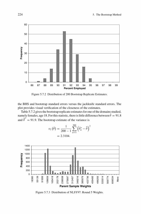
the BHS and bootstrap standard errors versus the jackknife standard errors. Theplot provides visual verification of the closeness of the estimates.

Table 5.7.2 gives the bootstrap replicate estimates for one of the domains studied,namely females, age 18. For this statistic, there is little difference between θ = 91.8

and ˆθ∗ = 91.9. The bootstrap estimate of the variance is

v2

(θ) = 1

200 − 1

200∑α=1

(θ∗α − ˆθ

)2

= 2.3104.

0

200

400

600

800

1000

1200

1400

18

38

0

55

13

9

91

89

9

12

86

59

16

54

18

20

21

78

23

89

38

27

56

97

31

24

57

34

92

16

38

59

76

42

27

36

45

94

95

49

62

55

53

30

14

56

97

74

60

65

34

Mor

e

Parent Sample Weights

Fre

qu

en

cy

Figure 5.7.3 Distribution of NLSY97: Round 5 Weights.

P1: OTE/SPH P2: OTE



0

200000

400000

600000

800000

1000000

1200000

1400000

0 200000 400000 600000 800000 1000000 1200000 1400000 1600000 1800000 2000000

Parent Sample Weights

Fir

st

Rep

licate

Weig

hts

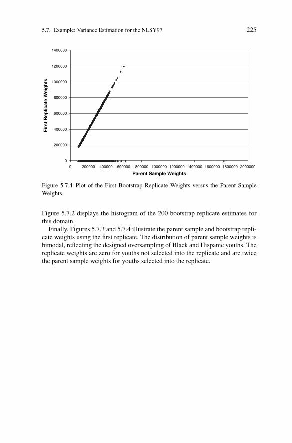
Figure 5.7.4 Plot of the First Bootstrap Replicate Weights versus the Parent Sample

Weights.

Figure 5.7.2 displays the histogram of the 200 bootstrap replicate estimates forthis domain.

Finally, Figures 5.7.3 and 5.7.4 illustrate the parent sample and bootstrap repli-cate weights using the first replicate. The distribution of parent sample weights isbimodal, reflecting the designed oversampling of Black and Hispanic youths. Thereplicate weights are zero for youths not selected into the replicate and are twicethe parent sample weights for youths selected into the replicate.

the bootstrap method kirk wolter

Documents