The Big Problem with Small ChangeThomas J. Sargent and François R. Velde

Working Papers SeriesResearch Department(WP-97-8)

Federal Reserve Bank of Chicago

Working Paper Series

The Big Problem of Small Change∗

Thomas J. Sargent

University of Chicago and Hoover Institution

Francois R. Velde

Federal Reserve Bank of Chicago

ABSTRACT

Western Europe was plagued with currency shortagesfrom the 14th to the 19th century, at which time a ‘standardformula’ had been devised to cure the problem. We use a cash-in-advance model of commodity money to define a currencyshortage, show that they could develop and persist under acommodity money regime, and analyze the role played by eachingredient in the standard formula. A companion paper docu-ments the evolution of monetary theory, monetary experimentsand minting technology over the course of six hundred years.

v1.0 October 1997

∗ The views expressed herein are those of the authors and not necessarily those of the Federal ReserveBank of Chicago or the Federal Reserve System.

1. Introduction

The title of this paper paraphrases one by Carlo Cipolla.1 Like Cipolla, our subject is the

process through which western monetary authorities learned how to supply small change.

Along with many other writers, Cipolla described how Western Europeans long struggled

to sustain a proper mix of large and small denomination coins, and to break away from

the idea that a commodity coinage requires coins of all denominations to be full-bodied.2

The Carolingian monetary system, born about A.D. 800, had only one coin, the

penny. At the end of the twelfth century, various states began also to create larger de-

nomination coins. From the thirteenth to the nineteenth century, there were recurrent

‘shortages’ of the smaller coins. Cipolla (1956, 31) states that: ‘Mediterranean Europe

failed to discover a good and automatic device to control the quantity of petty coins to be

left in circulation,’ a failure which extended across all Europe.3

By the middle of the nineteenth century, the mechanics of a sound system were well

understood, thoroughly accepted,4 and widely implemented. According to Cipolla (1956,

27):

‘Every elementary textbook of economics gives the standard formula

for maintaining a sound system of fractional money: to issue on government

account small coins having a commodity value lower than their monetary

value; to limit the quantity of these small coins in circulation; to provide

convertibility with unit money. . . . Simple as this formula may seem, it took

centuries to work it out. In England it was not applied until 1816, and in

the United States it was not accepted before 1853.’

Before the triumph of the ‘standard formula’, fractional coins were more or less

full bodied, and contained valuable metal roughly in proportion to their nominal values,

1 ‘The Big Problem of the Petty Coins’, in Cipolla (1956).2 The mix matters because small coins can make the same transactions as large coins, but not vice

versa. This is true so long as there is no ‘limited legal tender’ clause of the kind mentioned by Cipolla asa possible fourth element of his ‘standard formula’.

3 These shortages are documented in Sargent and Velde (1997b).4 For example, see John Stuart Mill (1857, chapter X, Section 2).

1

contradicting one element of the ‘standard formula.’ Supplies were determined by private

citizens who decided if and when to use metal to purchase new coins from the mint at

prices set by the government, contradicting another element of the standard formula. That

system produced chronic shortages of small coins, but also occasional gluts. Gradually

over the centuries, theorists proposed components of the ‘standard formula’; occasionally

policy makers even implemented some of them. Full implementation waited until 1816, in

Britain; and, over the following 60 years, in France, Germany, the United States and other

countries, culminating in the establishment of the ‘Classical Gold Standard’ with silver

and bronze or copper coinage as subsidiary money.

Our goal in this paper is to understand what made the medieval monetary system

defective, and why it took so long to implement the standard formula. We present a model

of supply and demand for large and small metal coins designed to simulate the medieval

and early modern monetary system, and to show how its supply mechanism lay vulnerable

to alternating shortages and surpluses of small coins. We extend Sargent and Smith’s

(1997) model to incorporate demands and supplies of two coins differing in denomination

and possibly in metal content. We specify cash-in-advance constraints to let small coins

make purchases that large coins cannot. Like the Sargent-Smith model, for each type of

coin, the supply side of the model determines a range of price levels whose lower and upper

boundaries trigger coin minting and melting, respectively. These ranges let coins circulate

above their intrinsic values. The ranges must coincide if both coins are to continue to

circulate. The demand side of the model delivers a sharp characterization of ‘shortages’

of small coins. ‘Shortages’ make binding our additional cash-in-advance constraint—the

‘penny-in-advance’ constraint that requires that small purchases be made with small coins.

This means that small coins must depreciate in value relative to large coins during shortages

of small coins. Thus in our model, ‘shortages’ of small coins have two symptoms: (1) the

quantity theory of money splits in two, one for large coins, another for small; and (2) small

coins must depreciate relative to large ones in order to render binding the ‘small change

in advance constraint’ and thereby provide a motive for money holders to economize on

small change. In conjunction with the supply mechanism, the second response actually

aggravates the shortage.5

5 The ‘standard formula’ mentioned by Cipolla solves the exchange rate indeterminacy problem

2

We use these features of the model to account for various historical outcomes,

and, among other things, to account for why debasements of small coins were a common

policy response to shortages of small change. Then we modify the original arrangement by

including one or more of the elements in the ‘formula’ recounted by Cipolla, and show the

consequences. We compare these consequences with the predictions and prescriptions of

contemporary monetary theorists, and with episodes in monetary history, in particular the

spectacular failure of a fiduciary coinage in 17th century Spain, and the lessons drawn by

contemporary observers. By way of explaining why it took so long to come to the ‘standard

formula’, we enumerate the theoretical, technological and institutional prerequisites for its

implementation.6 In a companion paper (Sargent and Velde 1997), we document how

‘theory’ was ahead of technology and institutions until 1816.

In her fascinating account of Britain’s adoption of the gold standard, Angela Redish

(1990) confronts many of the issues studied in this paper, and traces England’s inability to

adopt the gold standard before the 19th century to the problem of small change. She finds

that “technological difficulties (the threat of counterfeiting) and institutional immaturity

(no guarantor of convertibility)” were the main obstacles. According to Redish, Matthew

Boulton’s steam-driven minting press of 1786 overcame the first obstacle by finally giving

the government a sufficient cost advantage over counterfeiters. Redish identifies no such

watershed with respect to convertibility. Though she traces the Bank of England’s pro-

tracted negotiations with the Treasury over responsibility for the silver coinage, it is not

clear what the obstacle was, and how it was overcome. In her conclusion, Redish suggests

the earlier history of small change as a possible testing field for her theory. In some ways,

we are pursuing this project here.

This paper has a companion (Sargent and Velde 1997) that traces in detail the

histories of thoughts, technologies, and policies bearing on issues of coinage. That parallel

study motivated the questions and modeling decisions in the present paper.

inherent in any system with an inconvertible and less than full bodied fractional currency. Remember thatRussell Boyer’s (1971) original paper on exchange rate paper was titled ‘Nickels and Dimes’. See Karekenand Wallace (1981) and Helpman (1981) for versions of exchange rate indeterminacy in models of multiplefiat currencies. A ‘one-sided’ exchange rate indeterminacy emerges from the cash-in-advance restrictionsin our model, and determines salient predictions of the model.

6 We will also discuss a sense in which the formula has redundant elements.

3

The remainder of the paper is organized as follows. Section 2 describes the model

environment, the money supply arrangement, and the equilibrium concept. Section 3 uses

‘back-solving’ to indicate possible co-movements of the price level, money supplies, and

national income; to illustrate perverse aspects of the medieval supply arrangements; and

to interpret various historical outcomes. Section 4 uses the model to study how aspects of

Cipolla’s ‘standard formula’ remedy the perverse supply responses by making small change

into tokens. Section 5 concludes with remarks about how, by learning to implement a token

small change, the West rehearsed a complete fiat monetary system.

2. The Model

In a ‘small country’ there lives an immortal representative household that gets utility from

two nonstorable consumption goods. The household faces cash-in-advance constraints.

‘Cash’ consists of a large and a small denomination coin, each produced by a government-

regulated mint that stands ready to coin any silver brought to it by household-owned

firms. The government specifies the amounts of silver in large and small coins, and also

collects a flat-rate seigniorage tax on the volume of newly minted coins; it rebates the

revenues in a lump sum. Coins are the only storable good available to the household. The

firm can transform either of two consumption goods into the other one-for-one and can

trade either consumption good for silver at a fixed international price. After describing

these components of the economy in greater detail, we shall define an equilibrium. For

any variable we let x denote the infinite sequence {xt}∞t=0. Table 1 compiles the main

parameters of the model and their units.

4

Variable Meaning Units

φ world price of silver oz silver/cons good

b1 intrinsic content of dollar oz silver/dollar

b2 intrinsic content of penny oz silver/penny

γ1 melting point of dollar dollars/cons good

γ2 melting point of penny pennies/cons good

σi seigniorage rate (none)

b1−1 mint equivalent of dollar dollars/oz silver

b2−1 mint equivalent of penny pennies/oz silver

m1 stock of pennies pennies

m2 stock of dollars dollars

e exchange rate dollars/penny

p price of cons goods dollars/cons good

Table 1: Dramatis Personae.

The Household

The representative household maximizes

∞∑t=0

βtu (c1,t, c2,t) (1)

where we assume the one-period utility function u(c1,t, c2,t) = v(c1,t) + v(c2,t + α) where

α > 0 and v(·) is strictly increasing, twice continuously differentiable, strictly concave, and

satisfies the Inada conditions lim→0 v′(x) = +∞. We use consumption of good 1, c1, to

represent ‘large’ purchases, and c2 to stand for small purchases. There are two kinds of

5

cash: dollars, whose stock is m1, and pennies, whose stock is m2. Each stock is measured

in number of coins, dollars or pennies. Both pennies and dollars can be used for large

purchases, but only pennies can be used for small purchases.7 A penny exchanges for et

dollars. Thus, the cash-in-advance constraints are:

pt (c1,t + c2,t) ≤ m1,t−1 + etm2,t−1 (2)

ptc2,t ≤ etm2,t−1, (3)

where pt is the dollar price of good i. The household’s budget constraint is

pt (c1,t + c2,t) + m1,t + etm2,t ≤ Πt + m1,t−1 + etm2,t−1 + Tt, (4)

where Πt denotes the firm’s profits measured in dollars, and Tt denotes lump sum transfers

from the government. The household faces given sequences (p, e, T ), begins life with initial

conditions m1,−1, m2,−1, and chooses sequences c1, c2, m1, m2 to maximize (1) subject to

(2), (3), and (4).

Feasibility

A household-owned firm itself owns an exogenous sequence of an endowment {ξt}∞t=0.

In the international market, one unit of either consumption good can be traded for φ > 0

units of silver,8 leading to the following restrictions on feasible allocations:

c1,t + c2,t ≤ ξt + φ−1St, t ≥ 0 (5)

where St stands for the net exports of silver from the country.

Coin Production Technology and the Mint

7 The assumption that pennies can be used for the same purchases as dollars is motivated byseveral episodes in history during which small denominations overtook the monetary functions of largedenominations with great ease.

8 Alternatively, there is a reversible linear technology for converting consumption goods into silver.

6

Stocks of coins evolve according to

mi,t = mi,t−1 + ni,t − µi,t (6)

where ni,t ≥ 0, µi,t ≥ 0 are rates of minting of dollars, i = 1, and pennies, i = 2. The

government sets b1, the number of ounces of silver in a dollar, and b2, the number of ounces

of silver in a penny. The government levies a seigniorage tax on minting: for every new

coin of type i minted, the government charges a flat tax at rate σi > 0.

The country melts or mints coins to finance net exports of silver in the amount

St = b1 (µ1,t − n1,t) + b2 (µ2,t − n2,t) . (7)

Net exports of silver St correspond to net imports of φ−1St of consumption goods.

The quantities 1/b1 and et/b2 (measured in number of dollars per minted ounce of

silver) are called by Redish (1990) ‘mint equivalents’. The quantities (1− σ1)/b1, et(1 −σ2)/b2 are called ‘mint prices’, and equal the number of dollars paid out by the mint per

ounce of silver.

Government

The government sets the parameters b1, b2, σ1, σ2, and, depending on citizens’ mint-

ing decisions, collects revenues Tt in the amount

Tt = σ1n1,t + σ2etn2,t. (8)

Below we shall describe other interpretations of σi partly in terms of the mint’s costs of

production. The only modification that these alternative interpretations require would be

to (8).

The Firm

7

The firm receives the endowment, sells it, mints and melts, pays seigniorage, and

pays all earnings to the household at the end of each period. The firm’s profit measured

in dollars is

Πt =ptξt + (n1,t + etn2,t)− (σ1n1,t + σ2etn2,t)

− pt

(b1

φn1,t +

b2

φn2,t

)+ pt

(b1

φµ1,t +

b2

φµ2,t

)− (µ1,t + etµ2,t) . (9)

The first term measures revenues from the sale of the endowment; the next term is revenues

of minting, followed by seigniorage payments, minting costs, melting revenues and melting

costs.

The firm takes the price system (p, e) as given and chooses minting and melting

sequences (n1, n2, µ1, µ2) to maximize (9) subject to (6) period-by-period.

Equilibrium

A feasible allocation is a triple of sequences (c1, c2, S) satisfying (5). A price system

is a pair of sequences (p, e). A money supply is a pair of sequences (m1, m2) satisfying the

initial conditions (m1,−1, m2,−1). An equilibrium is a price system, a feasible allocation,

and a money supply such that given the price system, the allocation and the money supply

solve the household’s problem and the firm’s problem.

Analytical Strategy

We proceed sequentially to extract restrictions that our model places on co-movements

of the price level and the money supply. The firm’s problem puts restrictions on these co-

movements, and the household’s problem adds more.

Arbitrage Pricing Conditions

8

The firm’s problem puts the price level inside two intervals.9 Define γi = φ/bi and

rearrange (9):

Πt =ptξt +(1− σ1 − ptγ

−11

)n1,t + et

(1− σ2 − pt (etγ2)

−1)

n2,t

+(ptγ

−11 − 1

)µ1,t + et

(pt (etγ2)

−1 − 1)

µ2,t. (10)

Each period, the firm chooses ni,t, µi,t to maximize Πt subject to non-negativity constraints

ni,t ≥ 0, µi,t ≥ 0 and to the upper bound on melting: mi,t−1 ≥ µi,t, for i = 1, 2. The form

of (10) immediately implies the following no-arbitrage conditions:10

n1,t ≥ 0; = if pt > γ1 (1− σ1) (11a)

n2,t ≥ 0; = if pt > etγ2 (1− σ2) (11b)

µ1,t ≥ 0; = if pt < γ1 (11c)

µ2,t ≥ 0; = if pt < etγ2 (11d)

µ1,t ≤ m1,t−1; = if pt > γ1 (11e)

µ2,t ≤ m2,t−1; = if pt > etγ2. (11f)

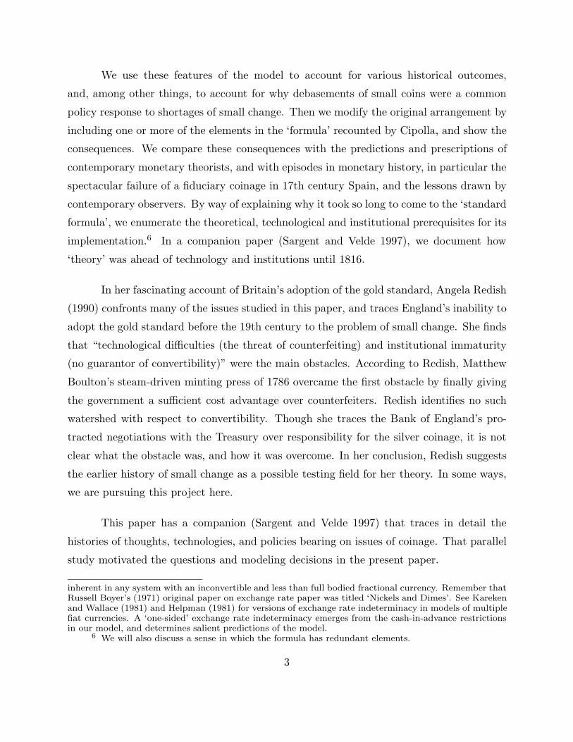
Implications of the Arbitrage Conditions for Monetary Policy

These no-arbitrage conditions constrain the mint’s policy if both coins are to exist.11

The constraints put pt within both of two intervals, [γ1(1 − σ1), γ1] (corresponding to

dollars) and [etγ2(1− σ2), etγ2] (corresponding to pennies). See Figure 1. Only when the

price level pt is at the lower end of either interval might the associated coin be minted.

Only when the price is at the upper end might that coin be melted. Therefore, if the lower

ends of the intervals do not coincide, (i.e., if γ1(1−σ1) 6= etγ2(1−σ2)), then only one type

9 See Usher (1943) for a discussion of these constraints on the price level.10 These restrictions must hold if the right side of (10) is to be bounded (which it must be in any

equilibrium); their violation would imply that the firm could earn unbounded profits.11 See the related discussion in Usher (1943, 1997–201).

9

of coin can ever be minted. Equating the lower ends of the intervals (by the government’s

choice of (bi, σi)) makes the mint stand ready to buy silver for the same price, whether

it pays in pennies or dollars. Equating the upper ends of the intervals makes the ratio of

metal contents in the two coins equal the exchange rate. If the upper ends of the intervals

don’t coincide, then one type of coin will be melted before the other. Pennies are said to be

full-bodied if 1/b1 = e/b2, that is, if the melting points (upper limits) of the two intervals

coincide. Household preferences and equations (2) and (3) imply that etγ2 ≥ γ1. If this

inequality is strict, the intrinsic content of pennies is less than proportionate to their value

in dollars, in which case pennies are ‘light’.12

dollars

pennies

γ1(1−σ1)γ1

eγ2e(1−σ2)γ2 pt

minting

minting

melting

melting

Figure 1: Constraints on the price level imposed by the arbitrage conditions.

Thus, if pennies are not full-bodied, a sufficient rise in the price level will make large

coins disappear. If the mint prices differ, a sufficient fall in prices will prompt minting of

12 By substituting Πt = ptξt, (8), and (6) into (4) we obtain

pt (c1,t + c2,t) ≤ ptξt + µ1,t + etµ2,t − (1− σ1) n1,t − et (1− σ2) n2,t.

Using the no-arbitrage conditions (11) in this expression and rearranging leads to

c1,t + c2,t ≤ ξt +hγ−11 (µ1,t − n1,t) + γ−1

2 (µ2,t − n2,t)i

.

The term in square braces equals net imports of consumption goods. Thus, as usual, manipulation ofbudget sets at equilibrium prices recovers a feasibility condition.

10

only one of the two coins. The perpetual coexistence of both coins in the face of price

fluctuations requires that pennies be full-bodied and that equal mint prices prevail for

both coins; that is, the intervals must coincide, and therefore the seigniorage rates must

be equal. This is not possible if we reinterpret the σi’s in terms of the production costs

for the two types of coins.

Interpretations of σi

In using (8), we have interpreted σi as a flat tax rate on minting of coins of type i.

But so far as concerns the firm’s problem and the arbitrage pricing restrictions, σi can be

regarded as measuring all costs of production borne by the mint, including the ‘seigniorage’

it must pay to the government. On this interpretation, in setting σi, the government is

naming the sum of the seigniorage tax rate and the mint’s costs of production. If a

government was unwilling to subsidize production of coins, then the costs of production

served as a lower bound on σi.

The government could decide to set gross seigniorage σi to 0, by subsidizing the

mint. In this circumstance, our two coins could coexist only if pennies were full-weight

(their intrinsic content being proportional to their face values), and if the price level never

deviated from γ1.

We discuss in the companion paper the attitudes of medieval writers as well as

the actual policies followed by governments. A tradition of thought advocated setting

σi = 0 but it was not followed in practice until the 17th century; other jurists thought

that σi should remain close to production costs, except in cases of clearly established fiscal

emergency.

On the other side, restraints were placed on the government’s freedom to set σi by

potential ‘competitors’ to the mint, such as counterfeiters and foreign mints, and by the

government’s ability to enforce laws against counterfeiting and the circulation of foreign

11

coins. Let σi be the production costs for counterfeiters, or for arbitrageurs taking metal to

foreign mints and bringing back coins (inclusive of transport costs). A wide gap between

σi and σi was difficult to maintain unless government’s enforcement powers were strong.

If they were not, σi placed an upper bound on σi.13

A government could maintain positive seigniorage if the costs of production of li-

censed mints were smaller than those of competitors. For example, Montanari ([1683]

1804, 114) argues that the death penalty for counterfeiting, while impossible to enforce

strictly, adds a risk premium to counterfeiters’ wage bill, thereby increasing σi when the

same technology is used by all. Furthermore, if a government was able to restrict access to

the mint’s technology, or if it could secure the exclusive use of a better technology, it could

set seigniorage above the mint’s production costs, up to the level of competitors’ costs.14

Per coin production costs differed between small and large denomination coins. The

Medieval technology made it significantly more expensive to produce smaller denomination

coins.15 In situations that tied the σi’s to the costs of production, different production

costs implied different widths of our no-arbitrage intervals. This meant either that pennies

had to be less than full-bodied or that the mint prices differed. In either case, price level

fluctuations could arrest production or, by stimulating melting, cause the disappearance

of one coin.

We have extracted the preceding restrictions from the requirement that equilibrium

13 See Usher (1943, 201): “Seigniorage presented no special problem unless the amount exceeded theaverage rate of profit attractive to gold and silversmiths, or to mints in neighboring jurisdictions. Beyondthis limit, the effective monopoly of coinage might be impaired by illegal coinage of essentially sound coins,or by the more extensive use of foreign coin.”

14 Philip II, king of Spain, referred explicitly to this advantage when he put a new technology to usein making small copper coinage in 1596. Mentioning the new mechanized mint of Segovia, he declared that“if we could mint the billon coinage in it, we would have the assurance that it could not be counterfeited,because only a small quantity could be imitated and not without great cost if not by the use of a similarengine, of which there are none other in this kingdom or the neighboring ones.”

15 This was true of competitors’ costs as well: Montanari notes that the risk premium induced bythe death penalty is the same across denominations. For arbitrageurs taking metal to foreign mints,transportation costs made the operation worthwhile only for the larger coins; the near-uniformity ofMedieval seigniorage rates on gold coins, contrasted with much greater variation on smaller coinage, bearsthis out.

12

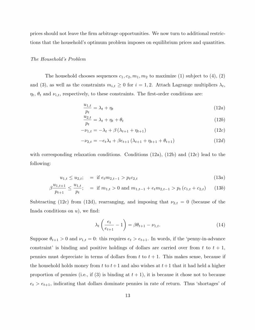
prices should not leave the firm arbitrage opportunities. We now turn to additional restric-

tions that the household’s optimum problem imposes on equilibrium prices and quantities.

The Household’s Problem

The household chooses sequences c1, c2, m1, m2 to maximize (1) subject to (4), (2)

and (3), as well as the constraints mi,t ≥ 0 for i = 1, 2. Attach Lagrange multipliers λt,

ηt, θt and νi,t, respectively, to these constraints. The first-order conditions are:

u1,t

pt= λt + ηt (12a)

u2,t

pt= λt + ηt + θt (12b)

−ν1,t = −λt + β (λt+1 + ηt+1) (12c)

−ν2,t = −etλt + βet+1 (λt+1 + ηt+1 + θt+1) (12d)

with corresponding relaxation conditions. Conditions (12a), (12b) and (12c) lead to the

following:

u1,t ≤ u2,t; = if etm2,t−1 > ptc2,t (13a)

βu1,t+1

pt+1≤ u1,t

pt; = if m1,t > 0 and m1,t−1 + etm2,t−1 > pt (c1,t + c2,t) (13b)

Subtracting (12c) from (12d), rearranging, and imposing that ν2,t = 0 (because of the

Inada conditions on u), we find:

λt

(et

et+1− 1

)= βθt+1 − ν1,t. (14)

Suppose θt+1 > 0 and ν1,t = 0: this requires et > et+1. In words, if the ‘penny-in-advance

constraint’ is binding and positive holdings of dollars are carried over from t to t + 1,

pennies must depreciate in terms of dollars from t to t + 1. This makes sense, because if

the household holds money from t to t+1 and also wishes at t+1 that it had held a higher

proportion of pennies (i.e., if (3) is binding at t + 1), it is because it chose not to because

et > et+1, indicating that dollars dominate pennies in rate of return. Thus ‘shortages’ of

13

pennies occur only after dollars dominate pennies in rate of return. To describe the rate

of return on pennies further, write (12c) and (12d) at t, and (12a) and (12b) at t + 1, and

make the necessary substitutions to obtain:

et

et+1=

u2,t+1

u1,t+1≥ 1. (15)

In models with only one cash-in-advance constraint but two currencies, this equation holds

with equality. Inequality (15) embodies a form of ‘one-sided’ exchange rate indeterminacy,

and leaves open the possibility of a class of equilibrium exchange rate paths that for which

the small change is not appreciating relative to large coins.

3. Equilibrium Computation via ‘Back-solving’

We utilize the same ‘back-solving’ strategy employed by Sargent and Smith (1997) to de-

scribe possible equilibrium outcomes. Back-solving takes a symmetrical view of ‘endoge-

nous’ and ‘exogenous’ variables.16 It views the first-order and other market equilibrium

conditions as a set of difference inequalities putting restrictions across the endowment, al-

location, price, and money supply sequences, to which there exist many solutions. We use

back-solving to display aspects of various equilibria. For example, we shall posit an equi-

librium in which neither melting nor minting occurs, then solve for an associated money

supply, price level, endowment, and allocation. We shall construct two examples of such

equilibria, one where the penny-in-advance constraint (3) never binds, another where it

occasionally does. We choose our sample equilibria to display particular adverse operating

characteristics of our money supply mechanism.

Equilibria with neither melting nor minting

When neither melting nor minting occurs, c1,t + c2,t = ξt, and mit = mi,−1 ≡mi, i = 1, 2. In this case, the equilibrium conditions of the model consist of one or the

16 See Sims (1989, 1990) and Diaz-Gimenez et al. (1992).

14

other of the two following sets of equations, depending on whether the penny-in-advance

restriction binds:

when (3) does not bind:

m1 + etm2 = ptξt

etm2 ≥ ptc2,t

c1,t + c2,t = ξt

u2,t

u1,t=

et−1

et= 1

u1,t

pt≥ β

u1,t+1

pt+1

or

when (3) binds at t:

m1 = ptc1,t

etm2 = ptc2,t

c1,t + c2,t = ξt

u2,t

u1,t=

et−1

et≥ 1

u1,t

pt≥ β

u1,t+1

pt+1

Notice how when (2) does not bind, there is one quantity theory equation in terms of the

total stock of coins, but that when (3) does bind, there are two quantity theory equations,

one for large purchases cast in terms of dollars, the other for small purchases in terms of

the stock of pennies.

In what follows, we begin by examining equilibria where the first set of conditions

applies at all times. We will show how to construct stationary equilibria. Then we will

study a variation in the endowment that brings into play the second set of equations,

when the penny-in-advance constraint binds, all the while maintaining the requirement

that neither melting nor minting occurs. Throughout, we take the mint policy (σi and γi)

as fixed.

Stationary Equilibria with no minting or melting

We describe a stationary equilibrium with constant monies, endowment, consump-

tion rates, price level, and exchange rate.

Proposition 1. (A stationary, ‘no-shortage’ equilibrium)

15

Assume a stationary endowment ξ, and initial money stocks (m1, m2). Let (c1, c2) solve

u1 = u2 (16)

c1 + c2 = ξ, (17)

Then there exists a stationary equilibrium without minting or melting if the exchange rate

e satisfies the following:

A = (γ1 (1− σ1) , γ1) ∩ (eγ2 (1− σ2) , eγ2) 6= /O (18)m1 + em2

ξ∈ A (19)

ξem2

em2 + m1≥ c2. (20)

Proof: Let p = (m1 + em2)/ξ. By (19), p will satisfy (11) in such a way that coins are

neither melted nor minted. Condition (2) is then satisfied with equality and (3) is satisfied

with inequality by (20). Since (3) does not bind, θt = 0 and conditions (12) are satisfied

with a constant e.

Condition (18), a consequence of the no-arbitrage conditions, requires that the

exchange rate be set so that there exists a price level compatible with neither minting nor

melting of either coin, of the type described in proposition 1. Condition (19) means that

the total nominal quantity of money (which depends on e) is sufficient for the cash-in-

advance constraint. Condition (20) puts a lower bound on e: the share of pennies in the

nominal stock must be more than enough for the penny-in-advance constraint not to bind.

Conditions (19) and (20) together imply that pc1 ≥ m1, that is, dollars are insufficient for

large purchases.

Figure 2 depicts the determination of c1, c2, p, and satisfaction of the penny in

advance constraint (3) with room to spare. There is one quantity theory equation cast

in terms of the total money supply. That there is room to spare in satisfying (3) reveals

16

ξ

ξ=c1+c2

c2

c1

C

F

U curve

slope: (et-1m2/m1)

expansion path

etm2/p

m1/p

Figure 2: Stationary equilibrium, non-binding constraint.

an exchange rate indeterminacy in this setting: a range of e’s can be chosen to leave the

qualitative structure of this figure intact. Notice the ray drawn with slope et−1m2m1

. So long

as the endowment remains in the region where the expansion path associated with a unit

relative price lies to the southeast of this ray, the penny-in-advance constraint (3) remains

satisfied with inequality. But when movements in the endowment or in preferences put the

system out of that region, it triggers a penny shortage whose character we now study.

Small coin shortages

Consistent with the back-solving philosophy, we display a few possible patterns of

endowment shifts that generate small coin shortages.

First, note that another way to interpret (19) and (20) is to take m1, m2, e as fixed

17

and to formulate these conditions as bounds on ξ:m1 + em2

γ1< ξ <

m1 + em2

γ1 (1− σ1)(21)

m1 + em2

eγ2< ξ <

m1 + em2

eγ2 (1− σ2)(22)

ξ ≤ αm1 + em2

m1 − em2(23)

(where (23) is written for the logarithmic utility case). These equations reveal a variety of

ways of generating small coin shortages with a change in ξ, starting from a given stationary

equilibrium. The simplest, which we explore first, is a one-time change in ξ within the

intervals defined in (21) and (22) but that violate (23): no minting or melting occurs, but

a shortage ensues. Another way is as follows: a shortage of small change arises when the

relative stock of pennies is insufficient relative to dollars (violation of (23)). Suppose the

lower bound in (22) is lower than that in (21). Then a shift in the endowment can lower

the price level to the minting point for dollars without triggering any minting of pennies,

resulting in a (relative) decrease in the penny supply; for some values of the parameters,

this can generate a shortage in the period following the minting of dollars.

Small coin shortage, no minting or melting

We begin by studying the situation that arises when, following an epoch where

constant money supplies and endowment were compatible with a stationary equilibrium,

there occurs at time t a shift in the endowment. In Figure 2, for the utility function

v(c1,t) + v(c2,t + α) we drew the expansion path traced out by points where indifference

curves are tangent to feasibility lines associated with different endowment levels. The

expansion path is c2 = max(0, c1 − α), and so has slope one or zero. If em2m2

> 1, i.e., if

pennies compose a large enough fraction of the money stock, then the ray c2/c1 equaling

this ratio never threatens to wander into the southeastern region threatening to render (3)

binding, described above. However, when em2m1

< 1, growth in the endowment ξ can push

the economy into the southeastern region, which makes (3) bind and triggers a depreciation

of pennies.

18

Thus, suppose that ξt is high enough that the intersection of the expansion path

with feasibility (c1+c2 = ξt) is above the ray et−1m2/m1. This means that at t, our second

subset of equations determines prices and the allocation. If we assume that ξt is such that

neither minting nor melting occurs (an assumption that must in the end be verified), then

equilibrium values of c1, c2, e, p can be computed recursively. Given et−1, the following

three equations can be solved for c1, c2, e at t:

c1,t + c2,t = ξt (24)u2,t

u1,t=

et−1

et(25)

etm2

m1=

c2,t

c1,t. (26)

These can be combined into a single equation in c2:

u1,t (ξt − c2,t, c2,t)u2,t (ξt − c2,t, c2,t)

=m1

et−1m2

c2,t

ξt − c2,t(27)

Define f(c2) = u2,tc2

ξ−c2

m1et−1m2

− u1,t. The fact that the expansion path intersects the

feasibility line below the ray et−1m2/m1 implies that f(c2) > 0 for (ξ − c2, c2) on the

expansion path. As c2 → 0, lim f(c2) < 0 (note that u2(ξ, 0) = u′(α) < +∞). Therefore,

there exists a solution c2 to (27). Then c1 is determined from (24), and et (which satisfies

et−1 > et by construction) is given by (25). It remains to check that pt = m1/c1 ∈ A and

that the Euler inequality βu1,t

pt≤ u1,t−1

pt−1holds. There is room to satisfy the inequality if

βpt−1pt

is small enough.

Figure 3 depicts the situation when constraint (3) is binding but no minting or

melting occurs. We use the intersections of various lines to represent the conditions (24),

(25) and (26), and to determine the position of the consumption allocation at point C.

The feasibility line F represents (24). Condition (26) means that the ray passing through

point C has slope etm2/m1: this defines et. Finally, condition (25) can be transformed

(using (26)) into the following:

c1 +u2,t

u1,tc2 = c1 +

et−1m2

m1c1. (28)

19

ξ

slope: -u2/u1

ξ=c1+c2

c2

c1

C

A

D

FR

c1+(u2/u1)c2 = c1+(et-1m2/m1)c1

U curve

slope: (et-1m2/m1)

Figure 3: Effect of a shift in endowments.

Define point A to be the vertical projection of C onto the ray et−1m2/m1. The left-

hand side of (28) is the point at which a line, parallel to the feasibility line and drawn

through point A, intersects the x-axis. The right-hand side is the point where the tangent

to the indifference curve at C intersects the x-axis. Condition (25) requires that these

intersections coincide. Note that, when the constraint does not bind, points A and C

coincide, and the tangent to the indifference curve coincides with the feasibility line.

Logarithmic example

Suppose in v(·) = ln(·) in equation (1). For this specification we can compute

pt, et, c1,t, c2,t by hand for the no-minting, no-melting case in which pt ∈ A, defined in

(18). When et−1m2m1

> ξt−αξt+α

, the constraint (3) does not bind; when the inequality is

reversed, it does bind, requiring a decrease in et relative to et−1. When (3) does not bind,

the time t equilibrium objects are c1,t = ξt+α2 , c2,t = ξt−α

2 , pt = m1+et−1ξt

. When (3) binds,

20

the solutions are c2,t = et−1m2m1−et−1m2

α, c1,t = ξt − c2,t, pt = m1/c1,t, et = ptc2,t

m2, where the

condition that et−1m2m1

< ξt−αξt+α implies that et−1 > et. It must be checked that pt ∈ A in

each case.

Permanent and transitory increases in ξ

Having determined the new exchange rate et after a shift in the endowment ξt, we

can determine what happens if the shift is permanent or transitory. If it is permanent,

then the constraint (3) will continue to bind. The reason is that, since et < et−1, the

ray etm2/m1 is in fact even lower than et−1m2/m1, which means that the expansion path

remains above the ray, and the penny constraint continues to bind. This situation cannot

continue without minting or melting indefinitely, however. Thus, a permanent upward shift

in the endowment from the situation depicted in Figure 2 to that in Figure 3 would impel

a sequence of reductions in the exchange rate until eventually the price level is pushed

outside the interval A.

As for a temporary (one-time) increase in ξt, it might prompt further depreciations

in the exchange rate even if the endowment immediately subsides to its original level. The

reason is that the reduction in et−1 induces a permanent downward shift in the em2m1

ray

that enlarges the (3)-is-binding southeastern region.

By shifting the interval for (e(1−σ2)γ2, eγ2) to the left, the reduction of et hastens

the day when pennies will be melted and postpones the day when they might be minted,

without a government adjustment of γ2. Not until the advent of the ‘standard formula’

described in the introduction was this perverse mechanism to be set aside.

Aggravated small coin shortage through minting of dollars

A shortage of small coins can also occur as a consequence of minting, independently

of the “income effect” we have described. Assume that all coins are full-bodied, so that the

21

bounds of the intervals coincide to the right (γ1 = eγ2), but that production costs require

that a higher seigniorage be levied on small coins (σ2 > σ1), so that the left boundaries

do not coincide (γ1(1− σ1) > eγ2(1− σ2)).

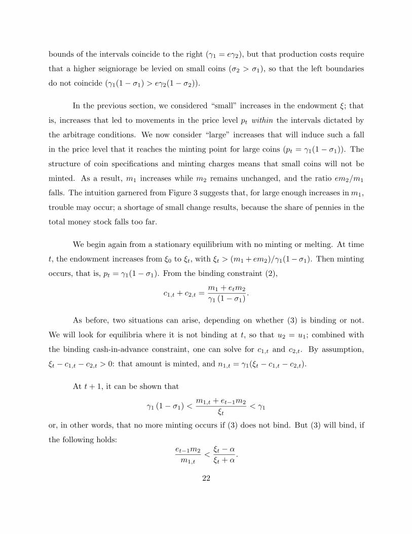
In the previous section, we considered “small” increases in the endowment ξ; that

is, increases that led to movements in the price level pt within the intervals dictated by

the arbitrage conditions. We now consider “large” increases that will induce such a fall

in the price level that it reaches the minting point for large coins (pt = γ1(1− σ1)). The

structure of coin specifications and minting charges means that small coins will not be

minted. As a result, m1 increases while m2 remains unchanged, and the ratio em2/m1

falls. The intuition garnered from Figure 3 suggests that, for large enough increases in m1,

trouble may occur; a shortage of small change results, because the share of pennies in the

total money stock falls too far.

We begin again from a stationary equilibrium with no minting or melting. At time

t, the endowment increases from ξ0 to ξt, with ξt > (m1 + em2)/γ1(1− σ1). Then minting

occurs, that is, pt = γ1(1− σ1). From the binding constraint (2),

c1,t + c2,t =m1 + etm2

γ1 (1− σ1).

As before, two situations can arise, depending on whether (3) is binding or not.

We will look for equilibria where it is not binding at t, so that u2 = u1; combined with

the binding cash-in-advance constraint, one can solve for c1,t and c2,t. By assumption,

ξt − c1,t − c2,t > 0: that amount is minted, and n1,t = γ1(ξt − c1,t − c2,t).

At t + 1, it can be shown that

γ1 (1− σ1) <m1,t + et−1m2

ξt< γ1

or, in other words, that no more minting occurs if (3) does not bind. But (3) will bind, if

the following holds:et−1m2

m1,t<

ξt − α

ξt + α.

22

This turns out to be a second-degree polynomial in ξt, which will be positive for large

enough values of ξt.

Thus, if enough dollars are minted, pennies become relatively short of supply.

Small coin shortages, secularly declining e

We have thus shown two ways that endowment growth can induce small coin short-

ages, with or without minting. We now discuss how such episodes affect the monetary

system over time, in particular the relation between small and large coins.

A shortage of small coins manifests itself in a binding penny-in-advance constraint

(3), and is associated with two kinds of price adjustments, one ‘static’, the other ‘dynamic’.

First, the quantity theory breaks in two to become two separate quantity theory equations,

one for small, another for large coins taking the forms pt = m1,t/c1,t and et = m2,t

ptc2,t. The

mitosis of the quantity theory is the time-t consequence of a shortage of small coins.

A second response is dynamic, and requires that et < et−1, so that pennies depreciate in

terms of dollars. This response equilibrates the ‘demand side’ but has perverse implications

because of its eventual effects on supply. For fixed b2, a reduction in e shifts the interval

[e(1 − σ2)γ2, γ2] to the left. This hastens the occasion when pennies will be melted, and

reduces the chances that pennies will again be minted.

This penny-impoverishing implication of a shortage-induced fall in e isolates a force

for the government to adopt an offsetting reduction in b2 eventually to resupply the system

with a new, lighter penny. Sargent and Smith’s (1997) analysis of a non-inflationary

debasement can be adapted to simulate such a debasement.17

An alternative way to realign the two intervals in response to a shortage-induced

17 This experiment stresses the ‘circulation by tale’ axiom embedded in our framework: for thepurposes of the cash-in-advance constraint (3), a penny is a penny. To analyze a debasement as describedin the text, one has to keep track of two kinds of pennies, old and new. See Sargent and Smith (1997) foran analysis in a one-coin system.

23

reduction in e would be to raise b1, thereby shifting the interval for large coins also to

the left. Such a small-coin-shortage-induced ‘reinforcement’ of large coins would evidently

diminish the price level.

1250 1300 1350 1400 1450 1500

101

102

lire

/ Flo

rent

ine

poun

d

grosso (60−80d)

picciolo (4d)

Figure 4: Plot of 1/b for two Florentine silver coins (1250–1530). The dots plot an indexof the price (in pennies) of the gold florin, or 1/et in our model.

While the model thus identifies either a debasement of small coins or a reinforcement

of large coins as a workable policy for keeping both large and small coins in existence,

history records more debasements of small coins. Cipolla reports secular declines in e

and b2, in the face of long periods of stable b1. For example, in Florence the gold florin

retained a constant metal content for centuries, while petty coins were recurrently debased.

Figure 4 plots the evolution of 1/b2 for two Florentine silver coins, the picciolo and the

grosso, during the Middle Ages (for the gold Florin, b1 remained constant). A pattern

of recurrent debasements, as describe by Cipolla, is apparent. The graph also displays

another piece of information, namely the price of the gold florin in terms of silver pennies:

24

this corresponds to 1/et in our model.18

The Affair of the Quattrini

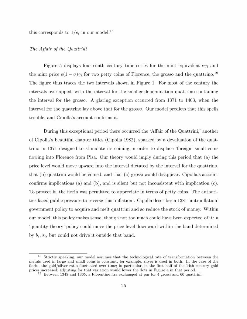
Figure 5 displays fourteenth century time series for the mint equivalent eγi and

the mint price e(1− σ)γi for two petty coins of Florence, the grosso and the quattrino.19

The figure thus traces the two intervals shown in Figure 1. For most of the century the

intervals overlapped, with the interval for the smaller denomination quattrino containing

the interval for the grosso. A glaring exception occurred from 1371 to 1403, when the

interval for the quattrino lay above that for the grosso. Our model predicts that this spells

trouble, and Cipolla’s account confirms it.

During this exceptional period there occurred the ‘Affair of the Quattrini,’ another

of Cipolla’s beautiful chapter titles (Cipolla 1982), sparked by a devaluation of the quat-

trino in 1371 designed to stimulate its coining in order to displace ‘foreign’ small coins

flowing into Florence from Pisa. Our theory would imply during this period that (a) the

price level would move upward into the interval dictated by the interval for the quattrino,

that (b) quattrini would be coined, and that (c) grossi would disappear. Cipolla’s account

confirms implications (a) and (b), and is silent but not inconsistent with implication (c).

To protect it, the florin was permitted to appreciate in terms of petty coins. The authori-

ties faced public pressure to reverse this ‘inflation’. Cipolla describes a 1381 ‘anti-inflation’

government policy to acquire and melt quattrini and so reduce the stock of money. Within

our model, this policy makes sense, though not too much could have been expected of it: a

‘quantity theory’ policy could move the price level downward within the band determined

by bi, σi, but could not drive it outside that band.

18 Strictly speaking, our model assumes that the technological rate of transformation between themetals used in large and small coins is constant, for example, silver is used in both. In the case of theflorin, the gold/silver ratio fluctuated over time; in particular, in the first half of the 14th century goldprices increased; adjusting for that variation would lower the dots in Figure 4 in that period.

19 Between 1345 and 1365, a Florentine lira exchanged at par for 4 grossi and 60 quattrini.

25

1300 1320 1340 1360 1380 1400 1420 1440 1460 148015

20

25

30

35

40

45

50

55

lira/

poun

d si

lver

grosso (30−80d)

quattrino (4d)

Figure 5: Evolution of the upper and lower bounds on quattrini and grossi, Florence.

4. Arrangements to eliminate coin shortages

This section describes two money supply mechanisms that, within the context of

our model, eliminate shortages of small coins. After briefly describing these mechanisms,

we will scrutinize them in terms of how they incorporate some or all of the ingredients

in Cipolla’s recipe, and will determine to what extent some ingredients of the recipe are

redundant.

A ‘standard formula’ regime

We change the supply mechanism to implement a version of Cipolla’s ‘standard

formula’, retaining the demand side of the model. It is as if the government tells the mint

to set up a ‘pennies department’ that operates like a ‘currency board’ for pennies. The

26

rules for supplying dollars are not changed from those described above. But now the mint

is required to convert pennies into dollars and dollars into pennies, upon demand and at

a fixed exchange rate e, named by the government. Assume that pennies are produced

costlessly by the mint, and so are truly tokens (b2 = 0). The government requires the

mint to carry a non-negative inventory of dollars Rt from each date t to t + 1. The mint

increases its inventory of dollars only when it buys dollars, and decreases it only when it

buys pennies.

This regime imposes the following laws of motion for stocks of dollars and pennies:

m1,t = m1,t−1 + n1,t − µ1,t − (Rt −Rt−1)

m2,t = m2,t−1 + e−1 (Rt −Rt−1)

Rt ≥ 0,

where Rt is the stock of dollars held by the mint from t to t + 1. The law of motion for

dollars can be rewritten as

(m1,t + Rt) = (m1,t−1 + Rt−1) + n1,t − µ1,t.

For the firm, it does not matter whether it melts dollars or whether pennies are exchanged

for dollars that are then melted; only the total stock of dollars m1,t + Rt counts.

Under this money supply mechanism, the firm’s profits become:

Πt = ptξt + n1,t − σ1n1,t − ptb1

φn1,t + pt

b1

φµ1,t − µ1,t, (29)

subject to the constraints n1,t ≥ 0 and m1,t−1 + Rt−1 ≥ µ1,t ≥ 0.

The absence of Rt from its profits signifies the firm’s indifference to the choice

of m2,t (as long as Rt ≥ 0), because the firm always breaks even when it buys or sells

pennies.20 The firm’s indifference lets the demand side of the model determine the stock

20 The condition Rt ≥ 0 can be ensured by choosing initial conditions such that em2,0 ≤ R0.

27

of m2,t appropriately. More precisely, one can find paths for the money stocks that are

consistent with the mint’s profit maximization and that satisfy the household’s first-order

conditions with (3) not binding.

A subset of the no-arbitrage conditions now obtains:

n1,t ≥ 0; = if pt > γ1 (1− σ1) (30a)

µ1,t ≥ 0; = if pt < γ1 (30b)

m1,t−1 + Rt−1 ≥ µ1,t; = if pt > γ1 (30c)

This regime forces pt into the interval [(1−σ)γ1, γ1]. In particular, pt can never rise above

γ1 because that would mean melting down all dollars, including those backing the pennies,

and the economy would have no money stock. This regime also solves the exchange rate

indeterminacy problem by administering a peg.

The positive stocks of Rt carried by the mint are socially wasteful, as indeed are

the stocks of silver being used in large coins.

Variants of the standard formula

The preceding version of a standard formula regime omits Cipolla’s stipulation to

‘limit the quantity of the small coins’ in circulation. Though our model renders that stip-

ulation redundant, various writers included them, and insisted on limiting the legal tender

of small coins and strictly limiting the quantity issued, often as supplements – though oc-

casionally apparently as alternatives to pegging the exchange rate et by converting either

coin into the other at par.

The effect of limited legal tender is evidently to modify the cash-in-advance con-

straint (2), because pennies are no longer accepted in payment of large purchases. Instead,

two separate cash-in-advance constraints are imposed.

28

The ‘standard formula’ without convertibility: the Castilian experience

One striking feature of the ‘standard formula’ and its reserve requirement is the

apparent wastefulness of Rt (in fact, of m1,t +Rt). We now consider a regime in which the

convertibility requirement is simply removed. As before, the rules for supplying dollars

are identical to the earlier ones. Pennies are token, that is, costless to produce. The

government does not require an inventory of dollars to back the pennies, but sets the

seigniorage rate on pennies σ2 = 1. The firm’s profit is then (29), to be maximized subject

to n1,t ≥ 0 and m1,t−1 ≥ µ1,t ≥ 0. Again, the firm is indifferent to the values taken by

µ2,t and n2,t. Those values are set exogenously by the government, and m2,t follows the

law of motion (6). The government’s budget constraint (8) is

Tt = σ1n1,t + etn2,t.

From the firm’s no-arbitrage conditions (30), we can bound pt below, by the minting point

γ1(1−σ1); but there is no upper bound on pt: if pt > γ1, µ1,t = m1,t and dollars disappear,

but pennies remain in circulation, and the cash-in-advance constraint (or quantity theory

equation) determines the price level:

pt (c1,t + c2,t) = etm2,t−1.

We start from given initial stocks m1,0 + em2,0 and a constant endowment ξ, such

that γ1(1 − σ1) < (m1,0 + em2,0)/ξ < γ1, and consider alternative policies for the path

of the penny stock. Suppose that a shift in endowment occurs as in section 3, so that no

minting or melting of dollars takes place. In the absence of any change in m2,0 a penny

shortage would develop. The shortage can be remedied, or prevented, by an appropriate

increase in m2, one that raises the ray of slope em2/m1 in Figure 2 so as to put the

intersection of the expansion path and the resource constraint in the southeastern region.

Issues of pennies can proceed in the absence of any further shifts in endowments.

Suppose ξ remains constant, but the government issues quantities of pennies every period.

29

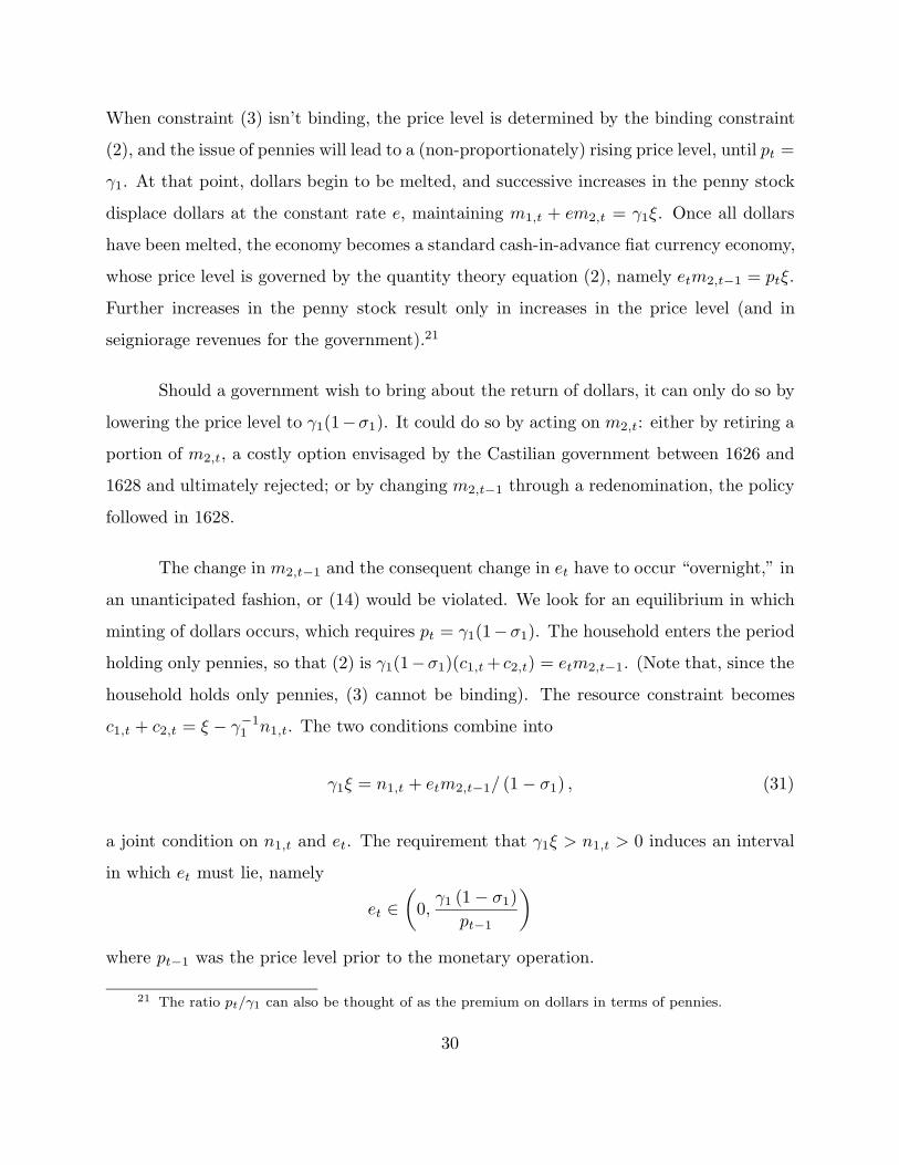
When constraint (3) isn’t binding, the price level is determined by the binding constraint

(2), and the issue of pennies will lead to a (non-proportionately) rising price level, until pt =

γ1. At that point, dollars begin to be melted, and successive increases in the penny stock

displace dollars at the constant rate e, maintaining m1,t + em2,t = γ1ξ. Once all dollars

have been melted, the economy becomes a standard cash-in-advance fiat currency economy,

whose price level is governed by the quantity theory equation (2), namely etm2,t−1 = ptξ.

Further increases in the penny stock result only in increases in the price level (and in

seigniorage revenues for the government).21

Should a government wish to bring about the return of dollars, it can only do so by

lowering the price level to γ1(1−σ1). It could do so by acting on m2,t: either by retiring a

portion of m2,t, a costly option envisaged by the Castilian government between 1626 and

1628 and ultimately rejected; or by changing m2,t−1 through a redenomination, the policy

followed in 1628.

The change in m2,t−1 and the consequent change in et have to occur “overnight,” in

an unanticipated fashion, or (14) would be violated. We look for an equilibrium in which

minting of dollars occurs, which requires pt = γ1(1−σ1). The household enters the period

holding only pennies, so that (2) is γ1(1−σ1)(c1,t + c2,t) = etm2,t−1. (Note that, since the

household holds only pennies, (3) cannot be binding). The resource constraint becomes

c1,t + c2,t = ξ − γ−11 n1,t. The two conditions combine into

γ1ξ = n1,t + etm2,t−1/ (1− σ1) , (31)

a joint condition on n1,t and et. The requirement that γ1ξ > n1,t > 0 induces an interval

in which et must lie, namely

et ∈(

0,γ1 (1− σ1)

pt−1

)where pt−1 was the price level prior to the monetary operation.

21 The ratio pt/γ1 can also be thought of as the premium on dollars in terms of pennies.

30

In the following period t1, neither minting nor melting occurs, because (31) implies

γ1 (1− σ1) ≤ n1,t + etm2,t−1

ξ< γ1

However, to ensure that (3) does not bind at t + 1, the stock of new dollars n1,t = m1,t+1

must not be too large: m1,t+1 ≤ pt+1ct+1, or (c2,t+1/ξ)n1,t ≤ etm2,t−1. This places a

further restriction on et, namely:

et ∈(

c2

c2 + (1− σ1) ξ

γ1 (1− σ1)pt−1

,γ1 (1− σ1)

pt−1

)(32)

where c2 lies on the expansion path and on the feasibility line in Figure 2.

Condition (32) requires the government to engineer a devaluation of pennies of the

“right” extent. If it is too small, no dollars are minted; if it is too large, too many dollars are

minted and another increase in m2 will be required to relieve the binding penny-in-advance

constraint.

We have assumed that the government carries out this operation in an unanticipated

manner. After 1628, the Castilian public surely viewed subsequent manipulations of m2

with some suspicion. Expectations of further reforms altered the demand for pennies, but

our simple model is not equipped to pursue the analysis in that direction.

Fiat Currency

To attain a version of Lucas’s (1982) model of fiat money, we would suspend the

original technology for producing both coins, and let them be produced costlessly. Al-

ternatively, we can think of ‘widening the bands’ – i.e., driving the γi’s to infinity. Like

Lucas, we would simply award the government a monopoly for issuing coins. We get a

pure quantity theory. The government fixes paths for mit, i = 1, 2, being careful to supply

enough pennies (i.e., to keep (3) from binding). Condition (2) at equality determines the

price level as a function of the total money supply. Condition (3) imposes a lower bound

on the quantity of pennies needed to sustain a fixed e equilibrium; equation (2) imposes

31

an upper bound on the amount of pennies that can be issued via ‘open-market operations’

for dollars.

5. Concluding Remarks

We designed our model to help us understand problems with the arrangements for minting

more or less full-bodied coins that prevailed for centuries throughout Western Europe. Our

model ascribes rules for operating the mint that copy historical ones, and focuses on the

difficulty those rules create for simultaneously maintaining two commodity currencies. The

model extends insights from single-currency commodity money models,22 where minting

and melting points impose bounds within which the price level must stay to arrest arbitrage

opportunities. In those one-commodity money models, when the price level falls enough

(i.e., when currency becomes scarce), new coins will be minted; and when the price level

rises enough, coins will be melted.23

With two currencies, there are distinct melting and minting points for each cur-

rency, and this causes trouble. We posit a particular model of demand for coins that, in

conjunction with the two sets of melting and minting points, makes shortages of the smaller

denomination coins arise when national income fluctuates. We analyze the perverse price

adjustments fostered by the historical supply arrangement, how they served to aggravate

shortages over time, and how they left debasement as the preferred relief.

The vulnerability to recurrent shortages of small coins that characterized the his-

torical supply arrangement eventually prompted its repair in the form of a huge ‘once-

and-for-all debasement’ of small coins, in the form of a permanent system of token small

change. In that system, the government acts as a monopolist for small coins. It can peg

the exchange rate of small for large coins, either by always choosing a proper quantity of

22 See Sargent and Smith (1997).23 Sargent and Smith (1997) analyze two-commodity monies in the form of gold and silver coins, but

do not link these metals to denomination as we do here. In particular, they have no counterpart to ourconstraint (3).

32

small ones, or by maintaining convertibility.

Establishing a system of token small change was a fateful step on the road to

creating a fiat money system for all currency. But refining the idea of fiat money and

actually implementing it were destined to take centuries. Historical episodes, such as

one in Castile in the 17th century, highlight the difficulty of establishing even a token

system for small coins in the face of technological imperfections, and of the pressures that

governments frequently had to raise revenues.

33

References

Cipolla, Carlo M. Money, Prices and Civilization in the Mediterranean World, Fifth to

Seventeenth Century. New York: Gordian Press, 1956.

Craig, John. The Mint: A History of the London Mint from A.D. 287 to 1948. Cambridge:

Cambridge University Press, 1953.

Diaz-Gimenez, J., Edward C. Prescott, T. Fitzgerald, and Fernando Alvarez. “Banking

in computable general equilibrium economies” Journal of Economic Dynamics and

Control 16 (March 1992): 533–560.

Glassman, Debra and Angela Redish. “Currency Depreciation in Early Modern England

and France” Explorations in Economic History 25 (January 1988): 75–97.

Helpman, Elhanan. “An Exploration in the Theory of Exchange-Rate Regimes” Journal

of Political Economy 89 (Oct 1981): 865–890.

Kareken, John H. and Neil Wallace. “On the Indeterminacy of Equilibrium Exchange

Rates” Quarterly Journal of Economics 96 (May 1981): 207–222.

Lucas, Robert E., Jr. “Interest Rates and Currency Prices in a Two-Country World”

Journal of Monetary Economics 10 (December 1982): 335–60.

Mill, John Stuart. Principles of Political Economy, Fourth Edition. London: John W.

Parker and Son, 1857.

Redish, Angela. “The Evolution of the Gold Standard in England” Journal of Economic

History 50 (December 1990): 789–805.

de Roover, Raymond A. La Pensee economique des scholastiques: doctrines et methodes.

Montreal: Institut d’Etudes medievales, 1971.

34

Sargent, Thomas J. and Francois R. Velde. “The Evolution of Small Change” Manuscript.

Chicago: Federal Reserve Bank of Chicago, 1997.

Sargent, Thomas J. and Bruce D. Smith. “Coinage, Debasements, and Gresham’s Laws”

Economic Theory (1997), forthcoming.

Sims, C. A.. “Solving nonlinear stochastic optimization and equilibrium problems back-

wards.” Institute for Empirical Macroeconomics, Federal Reserve Bank of Min-

neapolis: Working Paper 15, 1989.

Sims, C. A. “Solving the stochastic growth model by backsolving with a particular nonlin-

ear form for the decision rule” Journal of Business and Economic Statistics 8 (June

1990): 45–48.

Spengler, Joseph J. “Coin Shortage: Modern and Premodern” National Banking Review

3 (1966): 201–16.

35