Commodity and Token Monies

Thomas J. Sargent∗

November 2, 2018

Abstract

A government defines a dollar as a list of quantities of one or more precious metals.

If issued in limited amounts, token money is a perfect substitute for precious metal

money. Atemporal equilibrium conditions determine how quantities of precious met-

als and token monies affect an equilibrium price level. Within limits, a government

can peg the relative price of two precious metals, confirming Fisher’s (1911) response

to a classic criticism of bimetallism. Monometallism dominates bimetallism according

to a natural welfare criterion.

Keywords: Gold, silver, token money, bimetallism, quantity theory of money, gold ex-

change standard, (not a) fiscal theory of the price level

∗New York University, E-mail: thomas.sargent@nyu.edu. I thank Jeffrey Lacker, Francesco Lippi,Rodolfo Manuelli, Harald Uhlig, two referees, and editor Morten Ravn for helpful comments. I thankChenghan Hou and Ling Long for technical help.

1

1 Introduction

This paper analyzes (1) how supplies of two types of currency, one a precious metal, the

other a token, affect the price level; and (2) how two sources of demand for a precious

metal, one as a consumption good,1 the other as money, affect the price of the precious

metal relative to other consumption goods. These are two sides of the same coin. A

commodity money system binds the price level to the price of a precious metal relative

to other consumption goods.2 A government defines a dollar as a number of ounces of a

precious metal.3 Government or private agents might also issue tokens that exchange one-

for-one with money that is precious metal. Although they influence both the price level

and the allocation of metals between monetary and non monetary uses, limited amounts

of token monies are compatible with a commodity standard. But excess issues of token

money can sever the link between the price level and the price of a precious metal relative

to other consumption goods and thereby break a commodity standard. Nevertheless, David

Ricardo (1816) urged issuing the maximum amount of token money consistent with leaving

a commodity standard intact. We discuss Ricardo’s proposal in section 4.3.

Our analysis is old fashioned and entirely static despite theories of the demand for

currency naturally being intertemporal.4 Our justification for conducting a static analysis

is that instances of the atemporal inequalities that summarize the forces in our model

prevail in dynamic settings too, as readers of Barro (1979), Velde and Weber (2000), Velde

(2002) or the online appendix of this paper, for example, will recognize. We start with a

simple parametric theory of currency demand that we take for granted has emerged from a

dynamic theory, then focus on atemporal forces shaping demands for distinct objects, some

precious metals, others intrinsically worthless tokens, that comprise the currency stock.5

The heart of the theory is that, under appropriate circumstances, these objects are perfect

substitutes when used as money, but imperfect substitutes when not used as money.

We assume throughout that commodity monies are valued by weight and not by face

1Or maybe as an “industrial” good.2Or maybe a bundle of consumption goods.3Or in a multi-metallic standard, as given numbers of ounces of metal 1, metal 2, . . .. See section 5.4Therefore, our analysis leaves unmentioned intertemporal forces emanating from a sequence of govern-

ment budget constraints that are the focus of fiscal theories of inflation and the price level in the spiritof Sargent and Wallace (1981). In our framework, these forces would manifest themselves in the form ofpressures to adjust outstanding amounts of token money m.

5Assuming outcomes of a more comprehensive but unarticulated theory is what Leontief (1937) calledimplicit theorizing. He used that term to characterize and criticize Keynes’s General Theory. But theonline appendix sketches a dynamic model, the steady state of which matches our static analysis.

2

value.6 Section 2 describes open and closed economy models of a monometallic standard.

Sections 3 and 4 describe how the monometallic model expresses ideas and policy recom-

mendations of Smith (1937), Ricardo (1816), Fisher (1911), Hawtrey (1919), and others.

Section 5 describes a closed-economy model of a bimetallic standard. We use this model to

discuss the “Crime of ‘73” and how the suboptimality of bimetallism that prevails in the

model suggests that maybe those notorious events of 1873 should have been regarded not

as a crime but as a good deed. Appendix B contains proofs.

2 Monometallism

2.1 Cast of characters and units

A representative consumer enjoys two consumption goods, one that we call “standard”

consumption c, measured in units of that good, and silver s, measured in ounces. The

standard consumption good has one use. Silver has two uses because an amount s´ s ě 0

of silver is also used as money. There are competitive markets in silver and the standard

consumption good. The consumer’s preferences are ordered by upc, sq “ Acαs1´α, α P

p0, 1q, A ą 0. The ratio of the consumer’s marginal utilities for s and c is

ucus“

α

1´ α

s

c.

This ratio pins down the relative price of silver and the other consumption good. The

government defines a dollar as consisting of 1e

ounces of silver. The exchange rate e has

units of dollars per ounce of silver. The price of c relative to dollars is denoted p and is

measured in dollars per unit of the consumption good; p is also called the nominal price

level. The price of the standard consumption good relative to silver is pe, whose units are

ounces of silver per unit of consumption good. There is also a nonnegative amount of

token money m, whose units are dollars.7 When 0 ă s ă s, the total stock of currency is

M “ eps´ sq `m.

6Sargent and Smith (1997) and Sargent and Velde (2002) describe equilibria in which commodity moniesare valued by face value, i.e., “by tale”, instead of by weight.

7Milton Friedman was fond of calling token money “fiduciary” money.

3

2.2 Structural equations

The model has two structural equations, one imposing equality between demand for and

supply of real money balances, another imposing equality between demands for and supplies

of silver and the other consumption good:

eps´ sq `m

p“ kc, k ą 0 (1)

p

e“

α

1´ α

s

c(2)

Equation (1) is a “quantity theory of money” that equates the supply of real balances Mp

with the demand for real balances kc, where k is the “Cambridge k”.8 Equation (2) equates

the price of silver relative to the consumption good on the left side to the ratio of marginal

utilities ucus

on the right side.9

2.3 Closed and open economies

We study two versions of the model. In both we take the total supplies c, s as exogenous.

A small open economy version restricts c and s by

c´ c “ ´e

pps´ sq. (3)

In this version c, s are exogenous domestic endowments of the standard consumption good

and silver. They can be traded internationally subject to the budget constraint (3).

A closed economy version imposes

c “ c, s “ s. (4)

In this version, c, s are exogenous endowments of the standard consumption good and silver

that must be allocated domestically.

8See Johnson (1962).9The online appendix describes a dynamic version of the household’s optimization problem that would

emerge from a cash-in-advance constraint like those in Lucas (1982). The online appendix model assumesthat the standard consumption good is not durable and that silver is perfectly durable. A steady state ofthe associated dynamic model has versions of equations (1) and (2) that differ only in their constant terms.See equations (7) and (6) of the online appendix.

4

2.4 Open economy monometallism

The structural equations for the open economy model are (1), (2), and (3). Endogenous

variables are s, s, c and exogenous variables are p, e,m, s, c. Equilibrium c satisfies

c “α

1` kα

„

e

ps` c`

m

p

(5)

and equation (2) implies that equilibrium s is proportional to c:

s “p

e

1´ α

αc. (6)

To maintain convertibility of tokens for silver, m must respect

0 ď m ď kα

„

e

ps` c

. (7)

Equation (5) implies that if m “ 0

c “α

1` kα

„

e

ps` c

,

and that if m is at the upper bound in inequality (7) associated with retaining convertibility,

then

c “ α

„

e

ps` c

.

2.5 Closed economy monometallism

In the closed economy, c and s can be taken as exogenous by virtue of (4). We delineate

two regions of the parameter space.

In a first region, the quantity of token money m is small enough to allow the government

to peg the exchange rate e by defining a dollar as being worth (i.e., exchanging for) a

particular amount of silver. In this region, p, s are endogenous variables, while e,m, s p“

sq, c p“ cq are exogenous variables. Except at an upper bound on the stock of token money,

some silver is used as money.

In a second region, the quantity of token money is so large that no silver is used as money.

Here the endogenous variables are s, s, c while the exogenous variables are p, e,m, s, c. The

quantity of token dollars is too large to allow the government to succeed in naming e as

5

the quantity of silver that defines (i.e., that exchanges for) a dollar. No silver can be

exchanged for token money at the government mandated price e. Instead, it trades at a

price e determined by “the market”.

Proposition 2.1. To be in the first regime in which silver coins and tokens coexist as

money, the quantity of token money must respect the bounds:

0 ď m ď kα

1´ αse. (8)

Setting m ą k α1´α

se, puts the economy in the second regime in which silver trades for token

money at the exchange rate e “ 1´αα

csp ą e and the price level p satisfies m

p“ kc.

2.5.1 Equilibrium price level

Multiply equation (2) by p and combine the outcome with equation (1) to get two linear

equations in p and s. In the interior of the set of token money m values that satisfy (8),

solutions for s, p are

s “1´ α

1´ α ` kα

´

s`m

e

¯

p “α

1´ α ` kα

´es`m

c

¯

. (9)

The price level is an increasing function of m. Equation (2) captures the main force

leading to this outcome. Since e is fixed, equation (2) describes an increase in the price

level sufficient to bring about the reduced relative price of silver in terms of the standard

consumption good that is required by the increase in the equilibrium α1´α

sc

provoked by the

increase in m.

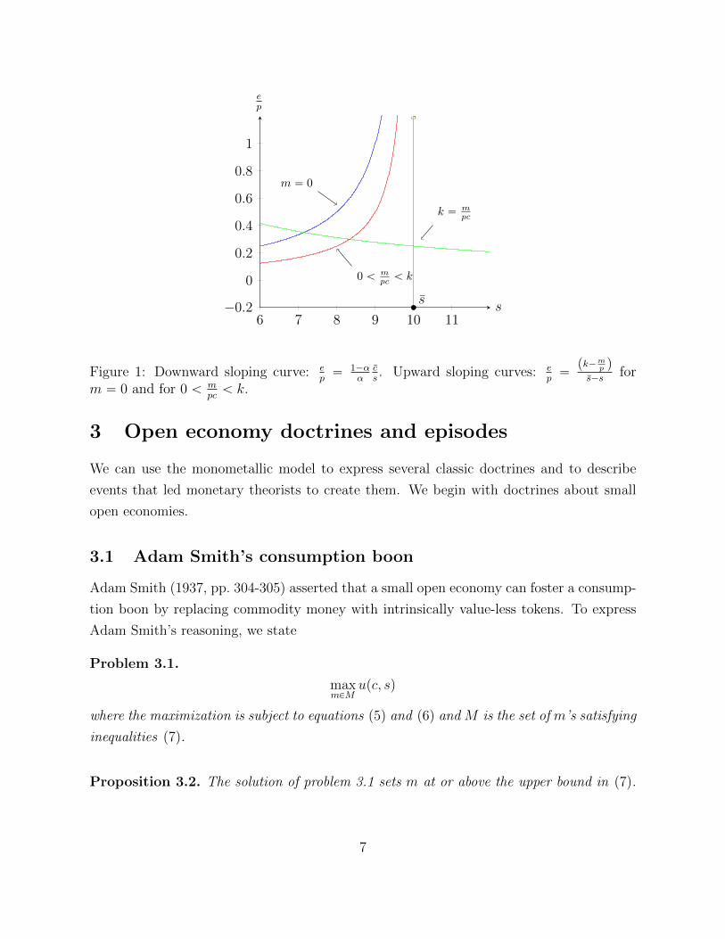
Figure 1 offers a graphical version of the closed economy model. The downward sloping

curve is a demand for nonmonetary uses of silver defined by equation (2). The upward

sloping curves are supplies of nonmonetary silver associated with different levels of mpcP

r0, ks implied by (1). Equilibrium ep

occurs at the intersection of demand and supply. Both

supply and demand curves are rectangular hyperbolas, demand with respect to s “ 0,

supply with respect to s´ s.

6

6 7 8 9 10 11´0.2

0

0.2

0.4

0.6

0.8

1

s

m “ 0

0 ă mpc ă k

k “ mpc

ss

ep

Figure 1: Downward sloping curve: ep“ 1´α

αcs. Upward sloping curves: e

p“pk´m

p qs´s

form “ 0 and for 0 ă m

pcă k.

3 Open economy doctrines and episodes

We can use the monometallic model to express several classic doctrines and to describe

events that led monetary theorists to create them. We begin with doctrines about small

open economies.

3.1 Adam Smith’s consumption boon

Adam Smith (1937, pp. 304-305) asserted that a small open economy can foster a consump-

tion boon by replacing commodity money with intrinsically value-less tokens. To express

Adam Smith’s reasoning, we state

Problem 3.1.

maxmPM

upc, sq

where the maximization is subject to equations (5) and (6) and M is the set of m’s satisfying

inequalities (7).

Proposition 3.2. The solution of problem 3.1 sets m at or above the upper bound in (7).

7

If m is lower than its upper bound in (7), small increments in m increase both c and s

but leave the price level unchanged. If m exceeds the upper bound in inequalities (7), the

market price of silver is e ą e and the price level p denominated in dollars is proportional

to m. In this case, units of account are dollars, which are not anchored to ounces of silver.

However, it is possible that the unit of account can remain silver even when m exceeds the

upper bound in inequalities (7). In this case, the price level measured in “silver dollars”

equals the exogenous “world price” p denominated in “silver” (a.k.a. the “hard currency”),

while “token” or paper money trades at a discount, exchanging for 1e

rather than 1e

vis a

vis the “hard currency.”

During both the US War of Independence and the US Civil War, paper money was

issued in amounts exceeding the upper bound in (7). During the first of these wars, paper

money traded at a discount relative to precious metal money, while during the second war,

precious metal coins traded at a premium relative to the government-issued paper money.

During the War of Independence, the unit of account continued to be the Spanish silver

dollar. After too many of them had been issued, paper dollars issued by the Continental

Congress depreciated relative to the Spanish dollar; eventually e rose by a factor of about

100. But commodity prices and bond contracts continued to be denominated in Spanish

dollars.10 By way of contrast, during the US Civil War, except on the West Coast, the unit

of account was a token money called the greenback dollar issued by the Union government.11

Goods prices and bond contracts were typically denominated in greenbacks. Gold dollars

traded at a premium over greenbacks, rising to over two greenbacks per gold dollar in 1864,

so that e was more than twice e and prices denominated in greenbacks rose approximately

proportionately with e.

Because our model is silent about what determines the unit of account, it cannot explain

why the precious metal coin remained the unit of account during the War of Independence

while the over-issued token currency became the unit of account during the Civil War. An

arrangement outside our model – the successful enforcement in Eastern and Midwestern

states of the legal tender provision of the 1862 Civil War Act authorizing greenbacks –

probably explains the difference.12

10For example, see the price series constructed by David and Solar (1977).11Rothbard (2002, pp. 127-128) describes how California and Oregon businessmen and courts maintained

the gold standard during the Civil War and accepted greenbacks only at discounts relative to gold dollars.12See Dewey (1912, ch. XII). Adams (1887, p. 144) noted that “by declaring its promises to be a legal-

tender in payment of private debts, the government virtually threatens to withdraw full protection inmatters of contract from every man who refuses to assist in floating its notes.”

8

3.2 “Too much token money”

Accounts of several inflation episodes – e.g., the North American War of Independence,

the North American Civil War – rest on calculating an upper bound on an amount of

token currency consistent with sustaining convertibility to precious metal at the official

exchange rate, like the one appearing in (7), as well as descriptions of inflations that

occurred when a government issued a token currency that exceeded that bound. Such

calculations typically consist of these parts: first, an estimate of the demand kc for real

balances during a hard money period immediately preceding large issues of token currency;

second, an estimate of additions to stocks of the token currency that would not imperil

its convertibility at par into precious metal coins; and third, an estimate of the date at

which issues of token currency passed the upper bound consistent with convertibility. For

example, the stock of specie circulating in the 13 North American colonies at the beginning

of the War of Independence was about 30 million Spanish dollars. In 1775, the Continental

Congress began issuing papers dollars. Each Continental dollar promised one Spanish

dollar. Continental dollars depreciated substantially relative to Spanish dollars only after

1776 when the Continental Congress had issued more than 30 million Continental dollars.

Estimates of kc for 1860 immediately before the U.S. civil were about 200 million dollars.

Gold and silver appreciated significantly relative to greenbacks only after the Union had

issued more than 200 million dollars of greenbacks.13

4 Closed economy doctrines and episodes

The “small open economy” doctrines and instances described in section 3 take as given the

relative price of silver and other consumption. We now turn to doctrines about a closed

economy. These are about effects of alterations in the stock of tokens on the relative price

of silver and other consumption goods.

4.1 Price level as relative price

When m “ 0, equation (30) tells us that an increase in the supply of silver increases the

price level, not through a “quantity theory” effect that makes p is proportional to m, but

13Sargent and Velde (2002, ch. 14) offer an account of an experiment in 17th century Spain in whichmoderate issues of copper token coins displaced silver but at first led to little inflation. But larger increasesin tokens caused substantial inflation. Sargent and Velde (2002, chs. 13,15) describe similar episodes inother countries.

9

by decreasing the price of silver relative to other consumption goods. Various authors used

that effect to explain rises in price levels after Spanish expropriations of silver and gold

from native Americans were brought to Europe during the 16th and 17th centuries.14 These

authors explained price level changes in terms of “ordinary microeconomics”, not a special

“monetary economics”.

When m ą 0 respects the bounds (7), equation (9) summarizes how increases in m

affect the price level by changing the relative price of goods for silver, an effect that we dub

a “Hawtrey effect”, to which we now turn.

4.2 Hawtrey effect

An analysis of price level determination based on formula (9) for the price level expresses a

line of causation of Hawtrey (1919) who described paths of nominal prices under England’s

convertible currency during the 1790s. After substantially increasing a paper currency

called the assignat in 1791 and 1792, France went on a paper standard; silver and gold

coins left France and pushed world prices of those precious metals downward relative to

consumption goods. That led to inflows of precious metals and upward pressure on British

prices. France returned to a specie standard in 1797 and precious metals flowed into France,

causing upward pressure on prices of precious metals and downward pressure on the British

price level. Hawtrey wrote about those 1790s events in 1919 because a number of countries

that had been on the gold standard before World War I had issued large amounts of currency

and abandoned convertibility to gold. Hawtrey meant to warn of the price level declines

that would come if all leading countries returned to the pre WWI gold standard at the old

par values. Hawtrey probably had in mind adverse effects on real activity coming through

a Phillips curve that is missing from the models in this paper.15

To avoid the adverse effects on real activity like those associated with France’s return

to specie in 1797 and Britain’s return to a specie standard in 1821 after the Napoleonic

Wars that he feared would accompany Britain’s return to gold after World War I, Hawtrey

embraced a recommendation of David Ricardo (1816) that we discuss next.

14See Parker (1974) and Sargent and Velde (2002, ch. 11).15Friedman and Schwartz (1963, ch. 7, sec. 4) and Friedman (1992, ch. 7) present an analysis of a

connection of President Roosevelt’s silver purchase program to a 1930s fall in the price level in China thatrests on this relative price effect. Rather than leading to a consumption boon in China, they assert that thefact that the price level is not “just another relative price” meant that the decline in Chinese prices causedadverse effects on real activity in China. Friedman and Schwartz are implicitly appealing to a Phillipscurve. Friedman (1992, ch. 7) critically reviews papers that had challenged evidence of adverse effects onreal activity in China coming from Roosevelt’s silver purchase program.

10

4.3 Ricardo’s proposal

We regard an influential proposal of David Ricardo as a refinement and extension of the

closed economy proposition 3.2 that we attributed to Adam Smith. Proposition 2.1 and

formula (33) in particular confirm Ricardo’s recommendation:16

The introduction of the precious metals for the purposes of money may with

truth be considered as one of the most important steps towards the improvement

of commerce, and the arts of civilised life; but it is no less true that, with the

advancement of knowledge and science, we discover that it would be another

improvement to banish them again from the employment to which, during a less

enlightened period, they had been so advantageously applied. Ricardo (1816,

p. 65)

To show how Ricardo’s recommendation manifests itself in our closed economy model,

we pose:

Problem 4.1.

maxmPM

upc, sq

where maximization is subject to equations (4) and (33) and M is the set of m’s satisfying

inequalities (8).

Proposition 4.2. The solution of problem 4.1 sets m at the upper bound, which in turn

assures that s “ s and s ´ s “ 0, thereby banishing silver as money, as Ricardo recom-

mended.

Thus, given e, welfare as measured by upc, sq is maximized by setting the supply of

token currency m at the upper bound associated with keeping token currency convertible

into silver coins at exchange rate e.17

4.4 A “gold-exchange standard”

Ricardo’s recommendation is the intellectual foundation of the normative case for the “gold

exchange standard” advocated by Hawtrey (1919) and others. To fix ideas, we use:

16This recommendation was adopted in various versions by Alfred Marshall, Irving Fisher, John MaynardKeynes, Ralph Hawtrey, and Milton Friedman.

17The Ricardo proposal to set mpc “ k at a fixed e to be discussed in section 4.3 drives the supply curve

in figure 1 toward a half rectangle with value zero and slope 0 for s ă s and slope `8 at s “ s.

11

Definition 4.3. In a “classical silver” standard, all money is silver, so m “ 0. In a pure

“silver exchange” standard, s “ s “ s, all money is token money, and token money m is

at the upper bound of inequalities (8).

When monetary historians write about a classical gold standard before World War I,

they have in mind that the metal s was “gold” rather than “silver” and that m was closer to

the lower bound in (8) than to the upper bound. When they write about the gold exchange

standard of the 1920s, they have in mind that m was closer to the upper bound.

5 Bimetallism

In this section, we describe a closed economy model of bimetallism. There are three distinct

utility yielding goods, namely, silver s, gold g, and standard consumption c. There are

potentially three types of currency: silver, gold, and token.18 At an interior equilibrium, the

three types of currency are perfect substitutes as money: token dollars are freely convertible

into gold or silver dollars at exchange rates eg and es named by the government. This aspect

of the model captures provisions of the US Coinage Act of 1792 that defined the dollar as

“371 4/16 grain (24.1 g) pure or 416 grain (27.0 g) standard silver” and the 10 dollar eagle

as “247 4/8 grain (16.0 g) pure or 270 grain (17.5 g) standard gold”.19

5.1 Background

A widely accepted criticism of bimetallism asserted: (1) that competitive markets determine

a relative price of silver for gold that responds to fluctuations in supplies of and demands

for gold and silver; (2) that if a government attempts to fix a time-invariant relative priceeges

, that relative price will almost always either over- or under-value silver relative to gold

relative to the price set by the market; and (3) that currency will be exclusively silver if it

is overvalued by the mint, and exclusively gold if it is overvalued by the mint.20

Fisher (1911) used geometry to construct a counterexample. He argued that within

well defined limits, by naming eges

, measured in ounces of silver per ounces of gold, the

18This is a poor man’s version of the Velde and Weber (2000) model of bimetallism. We eliminate all ofthe interesting dynamics and retain only the essential static “currency plumbing” that is at the heart oftheir model as well of the “diaphragm model” of Fisher (1911, ch. VII) that convinced Friedman (1990a,b).The key inequalities that drive the Velde and Weber (2000) and Fisher (1911) models are atemporal.

19Friedman (1951) analyses good properties of commodity monies.20A rallying cry of William Jennings Bryan and other advocates of bimetallism in the US during the

1890s was thateges

should equal 16.

12

government can set the market price of silver relative to gold in the face of sufficiently

moderate fluctuations in demands for and supplies of silver and gold. The shock absorber

at an interior equilibrium of Fisher’s model is that monetary uses of precious metals re-

spond to fluctuations in demands for non monetary uses. Our model expresses economic

forces underlying Fisher’s idea and also circumstances that render the preceding criticism

of bimetallism valid.21

5.2 The model

The utility function of a representative agent is upc, s, gq “ Acα1sα2g1´α1´α2 , where α1, α2,

and 1´α1´α2 are all in p0, 1q. Let p be the relative price of silver and consumption goods,

measured in ounces of silver per unit of consumption good, and let p be the relative price

of silver and gold, measured in units of ounces of silver per ounce of gold. The household’s

first-order necessary conditions for constrained maximization of upc, s, gq imply

ucus“ p

anducug“p

p.

The units of pp

are ounces of gold per unit of consumption good. Equilibrium relative prices

are

ucug“

α1

1´ α1 ´ α2

g

counces of gold per unit consumption

ucus“α1

α2

s

counces of silver per unit consumption

ugus“

1´ α1 ´ α2

α2

s

gounces of silver per ounce of gold (10)

The government names es and eg, whose units are dollars per ounce of silver and dollars

per ounce of gold, respectively. The amount of silver used as dollars is s´s and the amount

of gold used as dollars is g ´ g, where s, g are the total amounts of silver and gold used

either as dollars or for non-monetary pleasure (e.g., jewelry). Where m is the supply of

21Related representations of these same forces appear in Barro (1979) and Velde and Weber (2000).

13

paper dollars, the total supply of dollars is

M “ esps´ sq ` egpg ´ gq `m

and the quantity theory equation equating the supply of dollars to the demand is Mpc“ k.

In this closed economy model, s, g, and c are exogenous.22 The structural equations are:23

p

es“α1

α2

s

c(11)

p

eg“

α1

1´ α1 ´ α2

g

c(12)

esps´ sq ` egpg ´ gq `m

p“ kc (13)

We take as exogenous variables es, eg,m, s, g. Then we regard (11), (12), and (13) as three

equations to be solved for the three endogenous variables p, s, g.

5.2.1 A “natural” relative price

When k “ 0, there is no monetary demand for silver or gold. In that case, the price of gold

relative to silver is

φ “1´ α1 ´ α2

α2

s

g. (14)

The criticism of bimetallism against which Irving Fisher contended was that if the gov-

ernment were to set eges

at a value other than φ, then either gold or silver coins would

disappear. If egesą φ there would be only gold coins and if eg

esă φ there would be only

silver coins. All coins would consist of the metal that is “overvalued at the mint”, a version

of “Gresham’s law”.24 The heart of Fisher’s response is that when k ą 0, the presence of

monetary demands for gold and silver opens room for the government to set eges

not equal

22In a small open economy version, we would make endowments s, g, c exogenous, take the price level pas exogenous, and add a trade balance equation

pc´ cq `egppg ´ gq `

espps´ sq “ 0.

23Equation (13) incorporates a remark of Friedman (1951) that the real value of the stock of currency isindependent of the particular precious metal that is used as currency.

24For statements of Gresham’s law(s) that distinguish “circulation by weight” from “circulation by tale”,see Sargent and Smith (1997) and Sargent and Velde (2002).

14

to φ.

5.3 Interior equilibria with m “ 0

To begin, we follow Fisher (1911) and Velde and Weber (2000) by setting m “ 0 so that

money must be either gold or silver. An interior equilibrium respects the inequalities

0 ď s ď s (15)

0 ď g ď g (16)

At an interior equilibrium, algebra recovers the following formulas for s, g, p:25

s “

ˆ

α2

1´ α1 ` α1k

˙

ps`egesgq (17)

g “eseg

ˆ

1´ α1 ´ α2

1´ α1 ` α1k

˙

ps`egesgq (18)

p “

ˆ

α1

1´ α1 ` α1k

˙

´ess` egg

c

¯

(19)

Proposition 5.1. When m “ 0, inequalities (15) and (16) impose restrictions on the

government’s choice of eges

. We obtain an upper bound on eges

by equating s to s and solving

for eges

. We obtain a lower bound on eges

by equating g to g and solving for eges

. The bounds

are1´ α1 ´ α2

α2 ` α1k

s

gďegesď

1´ α1 ´ α2 ` α1k

α2

s

g(20)

At the upper bound, s “ s and at the lower bound g “ g. In the interior, s ă s and g ă g,

so that there are both gold and silver coins. As k “Ó 0, the bounds (20) collapse aroundeges“ φ, the “natural” relative price.

5.4 m ą 0 tightens the bounds on permissibleeges

We now consider how positive token money m ą 0 affects an interior equilibrium. Let

φ “ eges

. We begin by “back-solving” for an equilibrium in which eges“ φ, where φ is the

25Evidently, pes

pins down sc because p

es“ α1

α2

sc and p

egpins down g

c because peg“ α1

1´α1´α2

gc .

15

“natural” relative price of silver per unit of gold defined in equation (14). We seek an

equilibrium in which φ “ φ and in which there are neither silver nor gold coins. The price

of the standard consumption good relative to silver must be α1

α2

sc

because no silver is used as

money and the price of the standard consumption good relative to gold must be α1

1´α1´α2

gc

because no gold is used as money. If es is to be an active exchange rate in the sense

that es dollars actually exchange for an ounce of silver, then the price level has to satisfy

p “ p ” esα1

α2

sc. But for this to be the equilibrium price level, the stock of token money has

to satisfy m “ m ” kpc. If the money supply were less than m, there would be a “shortage

of money” and equation (13) would not hold at s “ s, g “ g. If more token money than

m were issued, then the price level would have to rise above p and token currency would

depreciate relative to the government set rate es.

This type of reasoning leads us to make the following

Proposition 5.2. There is an upper bound m on the stock of paper money that is consistent

with paper money exchanging for gold and silver at values eg and es set by the government.

At the upper bound, all money is token money and es and eg must satisfy eges“ φ, where

φ is the “natural” relative price of gold and silver defined in (14). The following steps tell

how to find the upper bound on m.

1. Set es ą 0

2. Set eg “ es1´α1´α2

α2

sg. (This sets eg

esto its “natural” value φ.)

3. Compute p “ esα1

α2

sc“ eg

α1

1´α1´α2

gc. Here p is an equilibrium price level that prevails

when there are neither gold nor silver coins, es dollars still buys one unit of silver,

and there is just enough token money to satisfy the demand for money at consumption

level c and nominal price level p.

4. Compute the upper bound m “ kcp; m is the amount of paper money that satisfies

the demand for real balances at the equilibrium price p.

At these settings of es and eg, s “ s, g “ g, p “ p and mpc“ k. Further, when 0 ă m ă m,

limits on eges

become

1´ α1 ´ α2

α2 ` α1pk ´mpcq

s

gďegesď

1´ α1 ´ α2 ` α1pk ´mpcq

α2

s

g(21)

16

Within these bounds, there is room to set eges‰ φ. At the upper bound, g “ g, at the lower

bound, s “ s, and inside the bounds, s´ s ą 0 and g ´ g ą 0.

Appendix A describes how to compute the equilibrium value of p when 0 ď m ď m. It

also provides formulas for equilibrium s and g.

5.4.1 Ricardo’s recommendation eliminates Fisher’s wedge

Inequalities (21) show that the lower and upper bounds on eges

both converge to the natural

relative price φ as mpcÒ k. Under the David Ricardo (1816) proposal to banish precious

metals from use as money by instead using tokens and thereby setting mpc“ k, the gov-

ernment loses the latitude to affect eges

that it has in the Fisher (1911)-Barro (1979)-Velde

and Weber (2000) model. Nevertheless, a policy that sets mpc“ k produces an equilibrium

allocation that maximizes upc, s, gq, reaffirming Ricardo’s recommendation.

5.5 Crime of ’73

We can use the model to represent the alleged “Crime of ’73” that occurred when Congress

took the United States from a bimetallic to a monometallic standard (see Friedman (1990a,b)).26

In this version of the model, the government declares that only gold, and not silver, can be

used as the commodity money. Convertible token money is still allowed. The government

defines a dollar as eg ounces of gold. Structural equations determining the price level p

now become

α1

p1´ α1 ´ α2q

g

c“

p

egegpg ´ gq `m

p“ kc. (22)

For simplicity, we focus on the pure gold standard case in which m “ 0 and compute the

following equilibrium values for g, s, p:

g “

ˆ

1´ α1 ´ α2

1´ α1 ´ α2 ` α1k

˙

g

s “ s

26In using a closed economy model, we are thinking about the early 1870s when France, Germany, andthe United States all left bimetallism for a gold standard.

17

p “

ˆ

α1

1´ α1 ´ α2 ` α1k

˙

egg

c. (23)

The equilibrium price of gold relative to silver is

ugus“

ˆ

1´ α1 ´ α2 ` α1k

α2

˙

s

g. (24)

Proposition 5.3. Compare an interior equilibrium of the bimetallic monetary system with

m “ 0 described in proposition 5.1 with an equilibrium of the monometallic monetary

system with m “ 0 described in this subsection. A comparison of formula (23) for the price

level under the gold-only economy with the price level (19) for the bimetallic economy shows

that the price level is lower under the monometallic gold-only economy. The price of silver

relative to gold is lower with the monometallic standard because more gold and less silver

is used as money, changing the amounts of gold and silver allocated to the non monetary

uses that determine the ratio of their marginal utilities.

Friedman (1990b) identified two 1890s constituencies that urged the United States to

return to bimetallism at a ugus“ es

egratio of 16 to one: silver producers, who sought an

increase in the relative price of silver, and debtors, who sought an increase in the price

level.27 Our model confirms the effects on both the price level and the relative price of

silver asserted by adherents to the “Crime of ’73” conspiracy story. But because it features

a representative agent, it fails to model the diverse interests that would have led some agents

to like and others to dislike those outcomes. Instead, as we see next, the representative

agent in our model would view Congress’s 1873 decision to demonetize silver as a blessing,

not a crime.

5.6 Sub optimality of bimetallism

The monometallic equilibrium in subsection 5.5 evidently sets eges

at or above the upper

bound of the interval defined by inequalities (20) so that s “ s and there are no silver coins.

While continuing to assume that m “ 0, we now seek a φ that respects the bounds (20)

27When the United States abandoned bimetallism in the 1870s, the price of silver relative to gold hadbeen approximately 16 to one. Velde (2002) gathered additional data and then reassessed and extendedFriedman’s analysis in terms of the Velde and Weber (2000) model.

18

and that yields equilibrium outcomes with maximum welfare measured by upc, s, gq.28,29,30

Proposition 5.4. Minimum upc, s, gq is attained by setting φ “ φ, the natural relative price

defined in equation (14). An interior equilibrium is dominated by both the s “ s monometal-

lic gold equilibrium at the upper bound of the interval (20) and the g “ g monometallic

silver equilibrium at the lower bound of the interval.

Evidently, a benevolent government always prefers φ at a corner. This occurs be-

cause the government’s choices of pg, s, φq are restricted by “implementability” conditions

in the form of equilibrium relationships, depicted by equations (17) or (25) and (18) or

(26), that describe how a representative agent adjusts non-monetary consumptions of sil-

ver and gold in response to alternative government choices of the price of silver relative to

gold φ. These implementability constraints confine the government’s choice of pg, sq to an

incentive-feasibility curve that is more concave than the representative consumer’s indiffer-

ence curve.31 Figure 2 indicates why an optimum is monometallic. The solid curve is the

locus of incentive-feasible pg, sq pairs, namely, pg, sq pairs that solve equations (17) or (25)

and (18) or (26) and are swept out by the implicit function theorem as the government’s

choice variable φ “ eges

moves from φ to φ, causing g to fall and s to rise as φ increases.

This is the set of ps, gq pairs from which the government chooses by setting φ P rφ, φs.

The three dotted lines are indifference curves, i.e., level curves of U “ Acα1sα2g1´α1´α2 .

For the parameters set in the figure, the highest indifference curve is attained at φ and is

affiliated with a monometallic silver standard solution g “ g. The lowest indifference curve

is attained by setting φ “ φ, the natural relative price defined in (14).32

Whether a benevolent government wants gold or silver to be used as money depends

on the representative consumer’s preferences. When α2 ą 1 ´ α1 ´ α2, i.e., when the

28This is our version of Proposition 2 of Velde and Weber (2000, p.1219). Our figure 2 is a counterpartto Velde and Weber’s Figure 2.

29A classic case for preferring bimetallism over monometallism argued that an average of the price goldrelative to other consumption goods and of the price of silver relative to consumption goods would be lessvolatile over time than either of those prices, providing a more stable price level. See Barro (1979) andFisher (1911).

30Manuelli and Wallace (1984) analyze the efficiency of commodity money equilibria in another setting.31This is thus an example of a Ramsey problem in which a “first-order approach” fails. Notice the role

of third derivatives in the Velde and Weber (2000, p. 1220) explanation for corner solutions.32At φ “ φ, g “ g, while at φ “ φ, s “ s. As φ increases in the interval φ P rφ, φs, s increases and

g decreases along the solid curve of incentive feasible pg, sq combinations. Because α2 ă 1 ´ α1 ´ α2, amonometallic silver money outcome that sets g “ g is optimal, given real balances of token money m

pc .

Minimum utility is attained at the natural φ “ φ that occurs at the tangency of an indifference curve withthe set of incentive-feasible pg, sq.

19

0.60 0.65 0.70 0.75 0.80 0.85 0.90 0.95 1.00g

6

8

10

12

14

16

s

Figure 2: Level curves of utility (dashed lines) and pg, sq combinations available to a gov-ernment that chooses φ “ eg

esP rφ, φs (solid line) for an economy with with α1 “ .3, α2 “

.2, A “ 1, c “ 10, s “ 16, g “ 1, k “ 1, mpc“ 0.0.

power coefficient on silver in the utility function exceeds the power coefficient on gold,

a monometallic gold standard dominates a monometallic silver standard. When α2 ă

1 ´ α1 ´ α2, a monometallic silver standard dominates a monometallic gold standard.

When α2 “ 1´α1´α2, the government is indifferent between the two possible monometallic

standards.

5.7 Gresham’s law

Equations equations (17) or (25) and (18) or (26) imply that in the interval pφ, φq, s is an

increasing function and g is a decreasing function of φ, the price of silver relative to gold

set by the government. At φ, g “ g and at φ, s “ s. If the government sets φ ą φ, the

consequence is that silver is “undervalued at the mint”, the market sets the price of silver

relative to gold at φ, s “ s, and all coins are gold. If the government sets φ ă φ, gold is

undervalued at the mint, the market sets the price of silver relative to gold at φ, g “ g, and

all coins are silver. These statements are versions of Gresham’s law, appropriately modified

to incorporate Irving Fisher’s response to critics of bimetallism.

6 Concluding remarks

The static models in this paper can help understand a variety of historical episodes and

policy decisions in addition to those described in sections 3, 4, and 5. For example, the

20

world price level stayed higher under the gold exchange standard after World War I than it

had been under the regime with less paper money that had been in place before 1914. That

outcome was an intended effect of Hawtrey’s recommendation to institute a gold-exchange

standard in the 1920s, an effect described by the analysis in section 4.2. Another example

is that for many years until 1871 France and other large countries were able to sustain a

bimetallic standard that kept the price of gold relative to silver pegged at about 15.5. The

“Fisher wedge” described by equation (20) in section 5.3 and equation (21) tells how they

could do that.33

The neglect of dynamics hard wired into our static models means that they have nothing

to say about important aspects of the episodes in monetary history mentioned here. Salient

among these are possibly interconnected issues about units of account and Phillips curve

dynamics that caused observers like Friedman (1992, ch. 7) to want more sophisticated

analysis of some of the episodes than we have provided.34

A Computing the price level when m ą 0

Equations (9) describe outcomes for the monometallic model. For the bimetallic model,

when 0 ă m ă m

s “α2ps`

egesgq

1´ α1 ´ α1mpc` α1k

(25)

g “eseg

p1´ α1 ´ α2qps`egesgq

1´ α1 ´ α1mpc` α1k

(26)

It follows that

s´ s “p1´ α1 ´ α2 ` α1pk ´

mpcqqs´ α2

egesg

1´ α1 ` α1pk ´mpcq

and

g ´ g “

esegpα1 ` α2 ´ 1qs` pα2 ´ α1pk ´

mpcqqg

1´ α1 ` α1pk ´mpcq

33The section 5.5 analysis explains how France’s and Germany’s 1871 abandoning of full bodied silvercoins contributed to a rise in the price of gold relative to silver.

34Doepke and Schneider (2017) present a model of units of account that emphasizes important featuresof economic environments ignored in this paper.

21

Substituting these expressions into the money market equilibrium condition (13) and rear-

ranging givesα1pk ´

mpcqpess` eggq

pp1´ α1 ´ α1pk ´mpcqq`m

p“ kc

which can be rearranged to become the following quadratic equation in p:

kcp1´ α1 ` α1kqp2` p´α1kpess` eggq ´mp1´ α1 ` α1kq ´ α1kmqp

`

ˆ

α1m

cpess` eggq ` α1

m2

c

˙

“ 0 (27)

B Proofs

Proposition 2.1:

Proof. We first consider the boundary at which m “ 0. Here only silver is used as money,

soeps´ sq

p“ kc. (28)

Equation (2) implies ep“ 1´α

αcs, which, substituted into (28) and rearranged, implies

s “s

1` α1´α

k. (29)

It follows thatp

e“

ˆ

α

1´ α ` αk

˙

s

c(30)

When m “ 0, p is proportional to e with k being a determinant of the factor of propor-

tionality. Here setting e is about units in which dollars are expressed: a change in e is just

a change in a unit of measurement. When equation (30) prevails, an exogenous increase in

the stock of silver s increases the price level by decreasing the price of silver relative to the

standard consumption good.

Next, we consider the other boundary at which mp“ kc. Here s “ s, so no silver is used

as money and all silver is enjoyed as an argument of upc, sq:

m

p“ kc (31)

22

p

e“

α

1´ α

s

c(32)

Use p “ α1´α

sc

and equation (31) to compute the following upper bound on token money m

that is compatible with a fixed e:

m ď kc

ˆ

α

1´ α

˙

s

ce.

So at a fixed e, m must respect the bounds (8). Within these bounds the amount of silver

enjoyed is

s “

ˆ

1`kα

1´ α

˙´1´

s`m

e

¯

. (33)

If m exceeds the upper bound in (33), the value of e set by the government becomes

inoperative – meaning that no one exchanges silver for token money at that exchange rate

and that traders instead exchange e ą e token dollars for an ounce of silver. Here s “ s

and a system of structural equations determining pp, eq is

m

p“ kc

e “1´ α

α

c

sp, (34)

the first being a pure quantity-theory equation that determines p as a function now purely

of the stock of paper m and the second stating that the dollar price of silver is proportional

to the price level.

Proposition 3.2:

Proof. Utility upc, sq is increasing in c and s. In the interval 0 ď m ď kα”

eps` c

ı

,

equilibrium c and s described by (5) and (6), respectively, are both monotone increasing

in m.

Proposition 4.2:

Proof. Evidently, in the interval 0 ď mpď kc, s “ s ´ p

epkc ´ m

pq attains it maximum s by

setting mp“ kc.

Proposition 5.4:

23

Proof. Choose φ to maximize upc, s, gq subject to equilibrium formulas for s and g appearing

in equations (17) and (18). The first-order necessary condition is usBsBφ` ug

BgBφ“ 0, where

the partial derivatives obtained from equations (17) and (18) are BsBφ“ α2

1´α1`α1kg and

BgBφ“

´p1´α1´α2q

1´α1`α1kφ´2s. Substituting these into the first-order condition, using formulas (25)

and (26), and rearranging gives φ “ 1´α1´α2

α2

sg, which equals the natural relative price φ in

equation (14) and lies in the interior of the set defined by the inequalities (20). The second

order condition verifies that this is a minimum. Moreover, where φ is the lower bound in

inequalities (20) and φ is the upper bound, usBsBφ`ug

BgBφă 0 when φ “ φ where g “ g, s ă s

and usBsBφ` ug

BgBφą 0 when φ “ φ where g ă g, s “ s.

References

Adams, H.C. (1887). Public Debts: an essay in the science of finance, New York: D.

Appleton and Co.

Barro, R.J. (1979). ‘Money and the Price Level under the Gold Standard’, Economic Jour-

nal, vol. 89(353), pp. 13–33.

David, P.A. and Solar, P. (1977). ‘A bicenenary contribution to the history of the cost of

living in american’, Research in Economic History, vol. 2, pp. 1–80.

Dewey, D.R. (1912). Financial History of the United States, 4th edition, New York: Long-

mans, Green, and Company.

Doepke, M. and Schneider, M. (2017). ‘Money as a Unit of Account’, Northwestern and

Stanford.

Fisher, I. (1911). The Purchasing Power of Money: Its Determination and Relation to

Credit, Interest and Crises, New York: Macmillan.

Friedman, M. (1951). ‘Commodity-reserve currency’, Journal of Political Economy,

vol. 59(3), pp. 203–232.

Friedman, M. (1990a). ‘Bimetallism Revisited’, Journal of Economic Perspectives, vol. 4(4),

pp. 85–104.

Friedman, M. (1990b). ‘The Crime of 1873’, Journal of Political Economy, vol. 98(6), pp.

1159–94.

24

Friedman, M. (1992). Money Mischief: Episodes in Monetary History, New York: Harvest

books, Houghton, Mifflin, Harcourt.

Friedman, M. and Schwartz, A.J. (1963). A Monetary History of the United States, 1867-

1960, Princeton, New Jersey: Princeton University Press.

Hawtrey, R.G. (1919). Currency and Credit, London: Longmans, Green, and Co.

Johnson, H. (1962). ‘Monetary theory and policy’, American economic review, vol. 52(3),

pp. 335–384.

Leontief, W. (1937). ‘Implicit theorizing: a methodological criticism of the neo-cambridge

school’, Quarterly Journal of Economics, vol. 51(2), pp. 337–351.

Lucas, R.J. (1982). ‘Interest rates and currency prices in a two-country world’, Journal of

Monetary Economics, vol. 10(3), pp. 335–359.

Manuelli, R. and Wallace, N. (1984). ‘Efficient and inefficient commodity “money” equilib-

ria’, Federal Reserve Bank of Minneapolis, Working paper 252.

Parker, G. (1974). ‘The emergence of modern finance in europe, 1500-1730’, in (C. M.

Cipolla, ed.), Fontana Economic History of Europe: The Sixteenth and Seventeenth Cen-

turies, .

Ricardo, D. (1816). Proposals for an Economical and Secure Currency, London: John

Murray, Albermarle-Street, reprinted in Vol. IV, of The Works and Correspondence of

David Ricardo, edited by Pierro Sraffa, with the collaboration of M.H. Dobb, Liberty

Fund, Indianapolis, 2004.

Rothbard, M.N. (2002). A History of Money and Banking in the United States: the Colonial

Era to World War II, Auburn, Alabama: Ludwig von Mises Institute.

Sargent, T.J. and Smith, B.D. (1997). ‘Coinage, debasements, and Gresham’s laws’, Eco-

nomic Theory, vol. 10(2), pp. 197–226.

Sargent, T.J. and Velde, F.R. (2002). The Big Problem of Small Change, Princeton, New

Jersey: Princeton University Press.

Sargent, T.J. and Wallace, N. (1981). ‘Some unpleasant monetarist arithmetic’, Federal

Reserve Bank of Minneapolis Quarterly Review, (Fall).

25

Smith, A. (1937). An Inquiry into the Nature and Causes of the Wealth of Nations, 1776,

New York: Modern Library.

Velde, F.R. (2002). ‘The crime of 1873: back to the scene’, Unpublished manuscript.

Velde, F.R. and Weber, W.E. (2000). ‘A Model of Bimetallism’, Journal of Political Econ-

omy, vol. 108(6), pp. 1210–1234.

26