the automatic sensing and analysis of three-dimensional
TRANSCRIPT


Digitized by the Internet Archive
in 2010 with funding from
University of North Carolina at Chapel Hill
http://www.archive.org/details/automaticsensingOOhenr


THE AUTOMATIC SENSING AND ANALYSIS
OF THREE-DIMENSIONAL SURFACE POINTS FROM VISUAL SCENES
by
Henry Fuchs
A dissertation submitted to the faculty of the
University of Utah in partial fulfillment of the requirements
for the degree of
Doctor of Philosophy
Department of Computer Science
The University of Utah
August 1975


IINIVEKSI'IY or UTAH GRADUA IK SC:ilO()I.
SUPERVISORY CO MM ITT HI-: APPROVAL
of a dissertation submitted by
Henry Fuchs
I have read this dissertation and hive found it icrhe of- satisfactory quality for adoctoral degree
i ^ I j "^
Robert P. PluiwrerChairman, Supervisory Coinmin*'
I have read this dissertation and have found it to be of satisfactory quality for adoctoral degree.
Steven V. CoonsMember. Supervisory Conunitiee
I have read this dis.-.enation and ha\c found it to be of satisfactoiy quality for adoctoral degree. 7 y 1 -'1 ^
Rate Elliott I. OrganickMember, Supervisory Committee

UNIVERSIl-Y OF UTAH GRADUATE SCHOOL
FINAL READING APPROVAL
To the Graduate Council of the Univcnity of Utah:
I have read the thesis ofHenry Fuchs
^ j^^ j^^.
final form and have found that ( 1 ) its fonnat, citations, and bibliographic style are
consistent and acceptable; (2) its illustrative materials including figures, tables, and
charts are in place; and (3) the final manuscript is satisfactory to the Supen/isory
Committee and is ready for submission to the Graduate School.
'^- (V7\
Robert P. PimninerMember, Super.'isory Committee
Approved for the Major Department
,^^^^'.^ /• ^.Anthony C. Hearn
Chairnian/Dean
Approved for the Graduate Council
Sterling M. McMurrinDem of Ihr Graduate School

ACKNOWLEDGMENTS
I am deeply grateful to my thesis supervisor, Robert Plummer, who has been a
constant source of assistance and encouragement throughout the course of this project.
I want to express my appreciation to the other members of the committee, Elliott
Organlck and Steve Coons, for many hours of discussions, suggestions and Insights ~ as
well as for responding so quickly and constructively to early drafts of this dissertation.
I would like to thank Ivan Sutherland, not only for being the initial inspiration for the
project, but also for serving as a committee member while he was still at Utah.
I would like to express my appreciation to Rich Riesenfeld and Elaine Cohen for help
and enthusiasm, especially at crucial periods in this project.
It should be noted that it is Mike Milochik to whom all praise is due for the excellent
photography, in spite of some less-than-excelient sources from which to work.
Thanks are due to the many friends and fellow students, who willingly lent their
bodies to be digitized in a none-too-comfortable environment.
Finally I would like to thank my parents for decades of faith, support, and
encouragement — without which none of this would have been possible.

TABLE OF CONTENTS
Acknowledgements iv
Abstract v"
Chapter 1 Introduction 1
1.1 Problem Statement 1
1.2 A Sampling of Previous Methods 2
1.2.1 Direct Manual Measurement 2
1.2.2 Mechanical Moving Devices 4
1.2.3 A Holographic Method 6
1.2.4 A Moire Method 8
1.2.5 Multiple 2-D Images 8
1.2.6 Controlled Illumination on Objects 14
Chapter 2 Design Philosophy 17
2.1 Hardware Design Considerations 19
2.2 Analysis System Considerations 20
Chapter 3 The Hardware Sensing System 21
Chapter 4 Data Acquisition, Analysis and Object Reconstruction 21
4.1 Basic Data Acquisition Programs 21
4.2 Analysis and Object Reconstruction Methodology 27
4.2.1 Sorting 28
4.2.2 Coherence 28

4.2.3 Applicability to the Present Situation 28
4.3 Description of Analysis and Reconstruction Algorithm 30
4.3.1 Analysis on Each Cutting Plane 33
4.3.2 Inter-Plane Reconstruction 37
Chapter 5 Conclusions and Further Development 47
5.1 Conclusions 47
5.2 Further Development 49
5.2.1 Hardware Improvements 49
5.2.2 Improved Analysis and Reconstruction Methods 51
Appendices 53
A. Descriptive List of Major Software Modules 53
B. Data File Formats 55
C. Sample Program Execution with Commentary 66
References 84

ABSTRACT
Described are the design and implementation of a new range-measuring sensing
dsvice end an associated software algoritf^m for constructing surface descriptions of
arbitrary three-dimensional objects from single or multiple views.
The sensing device, which measures surface points from objects in its environment,
is a computer-controlled, random-access, triangulating rangefinder with a
mirror-deflected laser beam and revolving disc detectors.
The algorithm developed processes these surface points and generates, in a
deterministic fashion, complete surface descriptions of all encountered objects. In its
processing, the algorithm also detects parts of objects for which there is insufficient
data, and can supply the sensing device with the control parameters needed to
successfully measure the uncharted regions.
The resulting object descriptions are suitable for use in a number of areas, such as
computer graphics, where the process of constructing object definitions has heretofore
been very tedious. Together with the sensing device, this approach to object
description can be utilized in a variety of scene analysis and pattern recognition
applications which involve interaction with "real world", three-dimensional objects.

CHAPTER 1
INTRODUCTION
1.1 Problem Statement
Researchers in seemingly-diverse areas are often concerned with the acquisition of
object descriptions. In artificial intelligence, for instance, a large part of most scene
analysis systems is devoted to generating a description of objects in the system's
working environment, whether this be a table-top scene of toy blocks, a rocky Martian
surface, or a work-station on an auto assembly line.
In computer graphics, much time is spent attempting to create accurate pictorial
images of real and imaginary objects. While the descriptions of imaginary objects are
often created with the aid of an associated computer-aided design system, the
descriptions of real objects usually has to be generated by laborious, largely-manual
measurement techniques.
The interest in object descriptions is not limited to computer users. A prosthesis
manufacturer may want to match the new artificial leg with the user's natural one, but
they may not have the facilities to take more than a few basic measurements.
Researchers in artificial intelligence (specifically robotics) have been among the ones
most intensely involved in the development of systems for the automatic acquisition of
object descriptions. Most of their systems, however, have relied on a picture-oriented
sensor, usually a TV camera. This report hopes to demonstrate that a significantly
different kind of sensor, a computer-controlled rangefinder, may also prove useful for

some of these tasks. The design and implementation of such a rangefinding system is
described. To demonstrate the feasibility of this approach, a simple scene-analysis
algorithm is implemented, which can generate, solely from the range data, descriptions of
objects in the sensor's field of view. It is hoped that this research will stimulate other
attempts at sensing systems more readily adaptable to the computer than the
human-oriented TV camera.
1.2 A Sampling of Previous Methods
1.2.1 Direct Manual Measurement
The most elementary method of digitizing objects is by direct, manual measurement.
With the aid of yardsticks, plumb lines and calipers, a great many solid objects can be
successfully measured, and the set of values later input to a computer system.
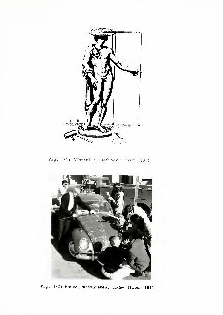
This idea of being able to specify an arbirarily complex three-dimensional object
with a set of simple measurements is hardly a recent development. The Renaissance
artist Leon Battista Alberti, in his book Delia Statua ,published in 1440, describes a
method for the accurate measurement of the human form (Figure 1-1). He claimed that
by using his method, different parts of the same statue could be constructed at separate
places and would still be able to fit together [10].
Today's approach, still basically the same, is often to mark all points of interest —
"key" points -- on the surface of the original object and then measure the distance of
each of these points from a common reference position (Figure 1-2). The surface is
then defined as a topological net over these key points. Of course, many tedious hours
must be spent to carefully measure the position of each selected point on the original
^g'^'^?;;^^.
Fig. 1-1: Albert! ' s "Definer" (from [10]
Fig. 1-2: Manual measurenent totiay (from [18])

ebject. The results are, however, often surprisingly effective. Although this method is
not practical for serious, large-scale digitizing, it should be noted that it has several
advantages over the other more sophisticated methods. Obviously, it requires almost no
equipment — hence no cost, except of course for manual labor. The resulting
descriptions also tend to be very compact, since the user naturally wants to minimize
the number of points that he has to measure. Although the less compact descriptions
resulting from the more sophisticated automatic methods can often be trimmed in size
according to some algorithm, it turns out that the subjective criteria used by humans are
usually more effective.
1.2.2 Mechanical Moving Devices
An obvious next step to the simple manual approach is to substitute some computer
sensing device for the user's calipers and yardsticks. The human user still has to define
the surface points and their interconnections, but now he can just move some pointer
around the object and tell the computer when the "current" position is of interest.
One device of this type is the so-called three-dimensional "crane" (Figure 1-3).
This is a mechanical arrangement of rods and gears which allows sliding movement in
each of the three axial directions. Through the amount of turning of each of three
gears, the computer can calculate the distance extended along each axis. The user
simply positions the tip of the crane's arm to a point of interest and instructs the
computer —through a foot switch in this case— to note the current position. Although
this method is much faster than the completely manual approach, it is still very
time-consuming. More serious is the severe limitation to the range of object sizes
which can be measured. Being a mechanical device, there are also considerations of its
bulkiness and the inertia and slippage of its moving parts.
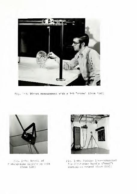
Fig. 1-3: Direct measurement with a 3-D "crane" (from [18])
ftsFig. l-4a: Detail of
fishing-line digitizing unit(from [20])
Fig. l-4b: Fishing line-connected
3-D digitizing handle ("wand")
restina on tripod (from [20])

A large variety of devices of this same general type have been constructed. One
such device has been in use at the University of Utah for a number of years [20]. It
uses three separate spring-loaded fishing-reel/fishing-line units (Figure l-4a). These
three assemblies are placed around the top corners of the working volume and the ends
of the three fishing lines are all connected to the tip of a pointing device (Figure 1-Ab).
From the amount of rotation on the shaft of each reel, the length of fishing line rolled
out can be calculated. Assuming that the lines are unobstructed, the three-dimensional
position of the pointer tip can be calculated from the three separate lengths of the
fishing lines.
1.2.3 A Holographic Method
Gara, Majkowski and Stapleton of General Motors Research Laboratories report the
development of a novel new digitization technique [8]. Although their system does not
have direct applicability to the interaction-oriented scene analysis applications, it may
provide a solution to the off-line object-digitization problem.
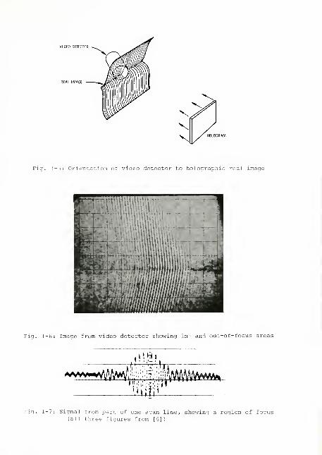
Their method consists of first taking a controlled, high-quality holograph of the
object of interest, then extracting surface measurements from the developed holograph
with a special-purpose computer-controlled video viewing system. The surface
measurements are calculated by moving the video detection sytem about the object's
holographic real image. As seen in Figure 1-5, there is a large angular orientation
between the face of the video detector and the object's surface image to allow both in
and out of focus parts of the image to hit the video detector's surface. The intersection
of the object's surface and the video detector's face is the locus of points on the
detector face at which the image is in sharpest focus. Figure 1-5 shows a typical video
image from the detector. (To aid in this focus-determination process, an optical
VIDEO DETECTOR
Fig. 1-5: Orientation of video detector to holographic real image
Fig. 1-6: Image from video detector showing in- and out-of-focus areas
(lb I
aN^ :^:myWywvwyvw
^M;.;j:;;;i
Fig. 1-7: Signal from part of one scan line, showing a region of focus(all three figures from [8]
)
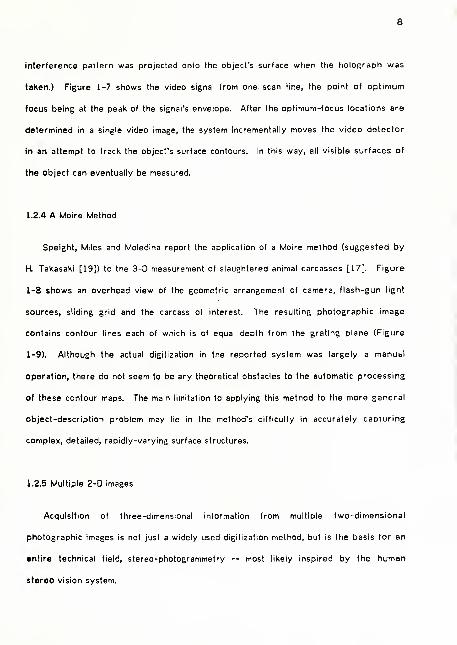
interference pattern was projected onto the object's surface when the holograph was
taken.) Figure 1-7 shows the video signal from one scan line, the point of optimum
focus being at the peaK of the signal's envelope. After the optimum-focus locations are
determined in a single video image, the system incrementally moves the video detector
in an attempt to track the object's surface contours. In this way, all visible surfaces of
tlie object can eventually be measured.
1.2.4 A Moire Method
Speight, Miles and Moledina report the application of a Moire method (suggested by
H. Takasaki [19]) to the 3-D measurement of slaughtered animal carcasses [17]. Figure
1-8 shows an overhead view of the geometric arrangement of camera, flash-gun light
sources, sliding grid and the carcass of interest. The resulting photographic image
contains contour lines each of which is of equal depth from the grating plane (Figure
1-9). Although the actual digitization in the reported system was largely a manuial
operation, there do not seem to be any theoretical obstacles to the automatic processing
of these contour maps. The main limitation to applying this method to the more general
object-description problem may lie in the method's difficulty in accurately capturing
complex, detailed, rapidly-varying surface structures.
1.2.5 Multiple 2-D Images
Acquisition of three-dimensional information from multiple two-dimensional
photographic images is not just a widely used digitization method, but is the basis for an
entire technical field, stereo-photogrammetry — most likely inspired by the human
stereo vision system.

FlnlliH
Fig. 1-8: Geometry for generating Moire patterns (from [17])
Fig. 1-9: Moire contour maps of 4 views of a lanb carcass (from [17])

10
The geometry is beautifully simple. If a picture of a ttiree-dimensional environment
is considered to be an image drawn on a window-pane in front of the viewer's eye, then
a point on that picture must correspond to a spot in the environment somewhere along
the line defined by the viewer's eye and the point on the image.
Given another eye-image pair at a different orientation to the object, and assuming
the point of interest is in view in both images, the point's three-dimensional position is
simply at the intersection of the two lines of sight (Figure 1-10).
A variety of methods are based on this simple idea. A common technique consists
of marking the points of interest on the object itself, then taking pictures from at least
two different viewpoints (Figure 1-11). If the camera/eye positions and orientations
are not known, they can be calculated from the correspondence between the picture
positions and the known 3-D positions of a number (at least 6) of "reference" points in
the object's environment [14].
When marking the subject is not practical, other methods can be employed. The
common practice is to take two pictures from locations only a small distance from each
other — similar to the two human-eye views. An operator then looks at these images
through a suitably adjusted stereo viewer and perceives the three-dimensionality of the
object. By moving a pointer in each view until they "merge" in the virtual
three-dimensional environment, he performs the correspondence which previously
consisted of manually marking the object. From the X,Y distances of the pointers in
each image, the three-dimensional position of the perceived point can be calculated [10]
An obvious advantage of this viewing approach is that an indefinitely large number of
points can be digitized, since with the marking method, only the actual points marked can
be measured. But with a stereo viewer, the accuracy of the measurements depends not

3-D object
Fig. 1-10: Triangulation from two images
Fig. 1-11: Actual digitization using two images with a data tablet
(from [18])

12
only on the interocular distance, but also on the visual acuity -- and the patience ! — of
the Operator.
Several attempts have been made to eliminate the need for the human operator to
specify the corresponce for each point to be measured. Levine et. al. [12] , expand
on an earlier algorithm of Julesz[ll] which is based on the observation that when two
views of a scene are taken from nearby positions, relative to the objects, then the
differences between corresponding parts of the two images is largely an X-axis offset,
with the amount of offset related inversely to the distance of the object from the
viewer (see Figure 1-12).
The technique then, is to digitize the two images and cross-correlate parts of
corresponding scan lines. The X offset of the best fit can be used to calculate the
three-dimensional position of the point defined by the center of the two matching
scan-line segments.
Some initial success has been reported with this method. The obvious difficulty is
that the viability of the offset-difference assumption (due to the depth-variation of the
object surface) is often inversely related to the distance of the object from the
viewing position; the assumption is reasonable for distant or flat regions where the view
from both eyes is essentially the same, but it is often invalid for close-by objects, as
with the face of a person , for whom one view may contain one side of the nose, and the
other view may contain the other side. On the other extreme, if the image of the local
surface is too similar in both images -- e.g. flat side of a building, a new sidewalk —
then there will also be difficulties due to a lack of characteristic features with which to
achieve a high cross-correlation.

\\\
left image \ i4j,
left eye
right image
right eye
Fig. 1-12: Cross-correlation of stereo images for depth determinatic
(inputs) (output)
Fig. 1-13: Object reconstruction from projected silhouettes (from [4])

14
As pari of a more extensive project on computer vision, Baumgart[3,'5] demostrates
a technique of reconstructing 3-D objects from tineir image silhouettes. The geometry is
similar to the triangulation technique m Figure 1-10, except that in this case instead of
line-of-sights being projected, the cone-shaped projections of a silhouette are mapped
into the object space. The object by definition is constrained to lie entirely within each
and every one of these projections. Baumgart describes it as being like "the old joke
about carving a statue by cutting away everything that does not look like the subject."
Figure 1-13 shows 3 silhouettes of a plastic horse and a view of the reconstructed
object. It is of interest to note that the input views were all from the horse's left side,
while the view of the reconstructed object is of the horse's right side. Due to the
projective nature of this method, however, surfaces with full concavities cannot be
adequately reconsfruted.
1.2.6 Controlled Illumination on Objects
Methods for extracting three-dimensional information from multiple two-dimensional
projections are not limited to considerations of photographs only. If the geometry of
Figure 1-10 is reconsidered, it can be observed that a pencil-beam of light can replace
one of the two lines-of-sights used in the triangulation process. In this way, one of the
photographs could be eliminated; the beam of light would be seen -- if not obscured by
some object -- as a bright reference point in the remaining photograph. This kind of a
system yields itself naturally to automatic processing; the origin and orientation of the
pencil-beam ot light can be placed under computer control and the photograph can be
input as a video picture. If the object under investigation can be examined at length,
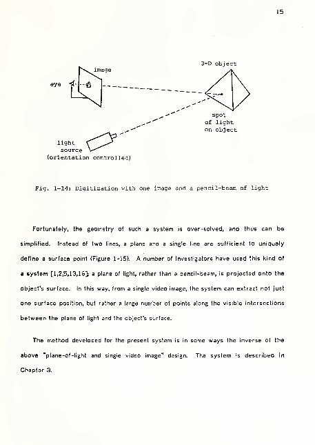
then an arbitrary number of points on its surface can be digitized (Figure 1-14).
15
3-D objectimage
light <:y(orientation controlled)
Fig. 1-14: Digitization with one image and a pencil-beam of light
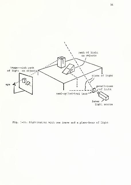
Fortunately, the geometry of such a system is over-solved, and thus can bo
simplified. Instead of two lines, a plane and a single line are sufficient to uniquely
define a surface point (Figure 1-15). A number of investigators have used this kind of
a system [1,2,5,13,15]; a plane of light, rather than a pencil-beam, is projected onto the
object's surface. In this way, from a single video image, the system can extract not just
one surface position, but rather a large number of points along the visible intersections
between the plane of light and the object's surface.
The method developed for the present system is in some ways the inverse of the
above "plane-cf-light and single video image" design. The system is described in
Chapter 3.
16
\ path of lightS on objects
image—with pathof light on objects.
eye
semi-cylindrical lens'
^ plane of light
\ pencil-beam
(P^o- light
laser r^
light source
Fig. 1-15: Digitization with one image and a plane-beam of light

CHAPTER 2
DESIGN PHILOSOPHY
It is important in design considerations to review not only what the present limited
system may be able to do, but also to delineate the scope ot capabilities desired for the
eventual "ideal" system.
is the basic goal of this research? It is to design a system v/hich can easily acquire
three-dimensional data and use it to construct surface descriptions of arbitrary
three-dimensional objects. The general idea is to build a system in which the hardware
sensor(s) and the software analysis algorithms interact to produce a more capable
system than would be possible without this interaction.
The desired system would have a sensor whose orientation to the object(s) could be
altered to allow input data from various views of the object. This could be
accomplished in a number of different ways. There could be several sensors mounted
at strategic locations around the system's environment. There could be a
system-controlled device — an arm, a turntable — which could move the object. The
sensor itself could be movable — on a track, on a computer-controlled arm, or mounted
on a moving platform. Of course, the particular application would influence the
configuration design. For example, the "moving platform" model would be the one most
likely to be used for a robotics application.
The scenario would go something like this. The object to be scanned is placed in
the system's environment. The sensor starts scanning the environment according to
some initial control parameters -- scanning the entire environment at a cursory level of
18
detail, or perhaps scanning only until a close-by object is encountered. The analysis
system — let's call it Analyzer — processes this initial scan data and begins to contruct
its object descriptions. These not yet being complete, Analyzer calculates the control
parameters the sensor needs to obtain the additional input data. The sensor again
gathers some data, now according to the new specifications. Analyzer processes the
new scan data and integrates it into its developing object-description structures. It
again determines whether it needs additional input data. If it does, it again calculates
the sensor control parameters. Again, the sensor is instructed to obtain more data,
according to its new set of control specifications. This interaction between the sensing
device and Analyzer continues until some "completeness" criterion in Analyzer is
satisfied.
This approach has several advantages over a simpler method. First, only the data
which is needed is actually acquired by the sensor. In this way, neither the sensor nor
Analyzer is burdened with unnecessary data. The level of detail can now vary with the
specific application. If the task is to give object descriptions to help navigate a robot
through an obstacle-filled environment, then one or two requests to the sensor may be
sufficient. If, on the other hand, the task is to digitize some arbitrary object for a
computer graphics system, then Analyzer could successively direct the sensor to those
regions of the object which have yet to be charted with adequate detail. The level of
input detail could also be context-dependent. If the objective is to inspect an
assemblage for missing bolts, then the level of detail could be modified as Analyzer
directs the sensor towards the regions of interest -- after, of course, it has located
these regions from earlier inputs.
19
2.1 Hardware Design Considerations
For an integrated system such as the one just described, the hardware system
should be as flexible as possible. Desired was a sensor which could acquire
three-dimensional surface data simply, and directly under computer control. An
accurate time-of-flight rangefinder would have been ideal, but, alas, too expensive. This
kind of system needs very high speed electronics which are capable of sensing the
delay between the time a pulse of laser light is started and the time its reflection
returns from the objects's surface. This may be as little as a few nano-seconds
(billionths of a second !). Time-of-flight rangefinders have been used to measure
distances from a few meters to thousands of kilometers.
For the present purposes, the most reasonable of the previous approaches seems to
be the "single image and a plane of light" method shown in Figure 1-15. Even with this
system, however, the degree of interaction between the data acquisition and the
analysis system is limited by the actual ("wall-clocK") time and the computer-processing
time commitment for an entire video image. Even if only one or two 3-D points are
needed, an entire video image has to be input. In order to extract 3-D information,
these systems must process the large amount of data inherent to a TV image. Although
they can extract many 3-D positions from each TV image, the rigid input pattern
required to do this — for example, having all points be co-planar -- may discourage
experimentation with analyses utilizing more context-dependent patterns of inputs, for
instance, those analyses for which the density of input data varies with the level of
interest in the local surface region. A system with efficient, explicit, single-point
measurement capability was judged more suitable forthe present effort.

20
2.2 Analysis System Considerations
Continuing the flexible approach to system design, it was decided that although
Analyzer may specify control parameters to the given input device, it should not depend
on interaction only with a particular kind of input device. Thus, for instance, when
Analyzer is connected to the proper input device, it can be constructing object
descriptions of buildings, automobiles, or microscope specimens. Also, while it can
always request more data for its description-building process, it should always be ready
to quit — i.e., the form of its object descriptions should be the same after the analysis
of one scan input as after ten. (These descriptions structures may, of course, abound
with "unknown" and "not sure" markers for much of the object's surface.) It is also
unrealistic to suppose that after each request to the input device, Analyzer will get the
exact data it requested. Due to obstacles m its way, or because of difficult surface
characteristics, the device may not be able to obtain the desired data; so Analyzer
should be able to integrate any new data which it gets.
The system should also be able to deal concurrently with more than one object in
the scene, and of course, there should be as little restriction as possible about the kinds
of objects which are acceptable; restrictions to planar-faced solids or simple geometric
shapes would be regrettable. As with any system operating in the "real world", the
analysis process should not fail simply because it gets some conflicts about its
environment -- e.g. different measurement values for the same surface from different
views. In short, a system was sought which would be simple, yet flexible and powerful
enough to allow implementation of a variety of experiments.

CHAPTER 3
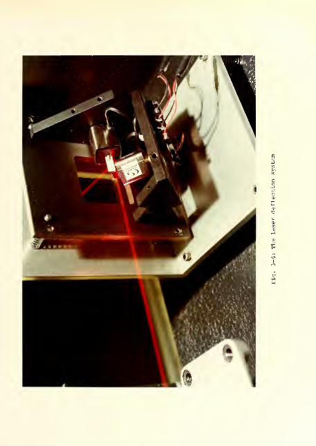
THE HARDWARE SENSING SYSTEM
The present sensor implementation is a simple, computer-controlled triangulating
rangefinder consisting of a mirror-deflected laser beam and spinning-disc detectors.
The spinning-disc detectors were previously developed by Robert Burton as part of a
PhD dissertation [6]. A basic description of his system will aid in understanding the
present implementation.
The objective of Burton's project was the rapid digitization of multiple
three-dlmensinal points of interest. The tip of a wand, the fingertips of a designer, the
key body points of a dancer can all be defined by the physical placement of very small
light bulbs -- actually Light-Emitting-Diodes (LED's) -- connected by thin wire to the
computer. With the room darkened, the computer, in sequence, turns on each of the
lights, at which time several widely-spaced detectors are asked to note the position of
the (only!) spot of light. By triangulating the data from several detectors, the
three-dimensional position of the small light can be determined. A naive approach
would have been to use TV cameras as detectors and find in each of the images the
position of the single spot of light. The actual implementation uses much simpler, more
efficient detectors than TV cameras. Each detector consists of a rapidly spinning disc
set between a wide-angle camera lens and a light-sensitive Photo-Multiplier (PM) tube
(see Figure. 3-1). The disc has radial slits cut at regular intervals, which at the proper
orientation allow the light passing through the lens to reach the PM tube. A reference
PM tube and reference light unit is added to monitor the slits as they pass by. From
this information, the exact position of a slit at any instant can be calculated. Now, since

22
the room is entirely dark except for the illumination of tfie one small LED of interest, ttie
only instant at which the PM tube senses any light is when the tube, a slit in the disc,
the lens and the LED are all lined up. Since the position of the slit at that instant can
be calculated from the reference PM tube data, the (unknown) position of the LED must
be somewhere on the plane defined by the positions of the slit, the lens, and PM tube
(see Figures 3-1,2,3). Since more than one of these sensors around the room is
expected to "see" the LED, its position is simply at the intersection of all these
detector-defined planes.
To modify this system into a computer-controlled rangefinder, a computer-deflected
laser beam was added to replace the LED's . The amount of laser light reflected from
most light surfaces was found to be sufficient to be noticed by the PM tubes in the
detectors. Now any surface point within the laser's (and the detectors') field of view
can be measured simply by aiming the laser beam in that direction. The deflection of
the beam is accomplished by reflecting the beam off two small front-surface mirrors
which are connected to the shafts of galvanometers mounted perpendicular to each
other (Figure 3-4). The control signals to drive the galvanometer electronics come
directly from the computer's digital-to-analog converters.
Although there are eight detectors m the present system -- two at each corner of
the room — it is easy to show that only one detector is actually necessary to obtain 3-D
surface positions. Since the laser deflection system is under computer control, and the
physical position of this unit in the room can be determined, the definition of the
laser-beam line can be calculated directly from the current X and Y deflections. Now,
since each detector identifies a plane through the room in which the spot of light must
lie, the spot has to be at the intersection of this plane and the laser-beam line.
(Because the present implementation has the luxury of using eight detectors, knowledge

spinning disc
Reference light
(enclosed)
Reference PM tube
radial slits (32 in all)
spot of light(in darkened room)
Fig. 3-1: A spinning disc detector and a spot of light
Reference PM tube (in back) y^-;'~v position of slit at which the
enclosed reference light / '\rS ^ reference light is allowed to
(in front) / y %\/' shine through to the"^^^^v Reference PM tube
~
Main PM tube (in back)
lens (in front)
(upside-down) image
of room cast by the lens
onto the planeof the disc
position of slit at which the light(from the single spot of light in the room)
is allowed through to the Main PM tube
/image of the spot of light
Fig. 3-2: Details of spinning disc detector
Signal from Main PM tube
Signal from Reference PM tube —(C is the primary inputto the 3-D calculations)
I slit now at Reference Assembly
lZ^X"
Fig. 3-3: Primary signals from the detector system

24
of the laser-beam of light In the environment is not used in the 3-D calculations.)
It Is Important to distinguish this kind of a digitizing system from the similar ones
described In Chapter 1. First, in place of the spinning disc detectors, TV cameras could
have been used, similar to the "single spot of light and the single image" method shown
in Figure 1-14. The primary advantage of the present disc detectors over TV cameras
is their speed and simplicity. A disc (with 32 radial slits) spinning at 3500 r.p.m. scans
the environment approximately 1900 times each second, as compared with the
approximately 30 frames each second acquired by the standard TV camera. Also, as can
be seen from Figure 3-3, each scan directly produces a single number ("C") for
processing, bypassing the need to handle the approximately 250,000 points in each
video frame.
Comparisons to the slightly different method of the "single image and a plane of
light" (Figure 1-15) are somewhat more involved. The digitization rate of this method is
substantially improved by being able to process many points (all along the plane of
light) from a single video image. The orientation of the plane of light, however, can only
be changed between video frames, perhaps each 1/30 of a second; so the system is
"committed" to an orientation for a large number of points. With the present
random-access laser-beam system, this commitment is only for a single point; so the
orientation of the beam can be changed "on the fly." This feature is especially important
for those applications in which the digitization of the scene is context-dependent, that is,
one in which each deflection position of the laser beam may be a function of the
previously calculated 3-D positions.


CHAPTER 4
DATA ACQUISITION, ANALYSIS AND OBJECT RECONSTRUCTION
The implemented programs consist of an interlocking set of modules, from those
which directly control the sensing system to those which analyze the data and generate
the actual object descriptions.
4.1 Basic Data Acquisition Programs
Since the laser deflection system is completely under computer control, a set of
programs specify control parameters to the hardware system. These parameters are
calculated from higher-level specifications obtained from the human operator. The
operator can specify the subregion in the laser deflection system's field of view which is
to be scanned. He can also specify the number of positions in the horizontal and
vertical directions for which measurements should be tal^en.
Due to the primitive nature of the present scanning system, a number of strategies
have been implemented in hopes of improving the accuracy of the input measurements.
A multiple number of measurements are usually taken at each deflection position of the
laser. The resulting measurements are then used to calculate a single more reliable
value, in addition, if the laser spot is not "seen" by enough of the sensors for a
minimum number of these attempts, then no final value is recorded for that particular
laser position. Another filter traps any value which falls outside of the specific
"working volume" of the scene. (A more detailed explanation, along with actual Teletype
listings of the programs in execution, is provided in Appendix C.)
27
4.2 Analysis and Object Reconstruction Methodology
While a number of different uses can be found for ttiis unusual sensing systerr), it
was decided that the task of object reconstruction would be an appropriate first
application. The term object reconstruction Is used here to mean the generation of
complete, closed surface topologies, defined by a connected set of polygonal tiles, which
approximates the surface data acquired from one or more views of the objects in the
environment. Although this task has many similarities to the much-researched scene
analysis problem in artificial intelligence, the present implementation has a somewhat
different orientation in that it makes almost no assumptions about the specific kinds of
objects it expects to find. This feature can be viewed as an advantage in favor of
generality, but of course it also prevents the system from making many inferences from
partial data -- concerning, for example, the likely location and characteristics of
obscured surfaces.
Early in the project a similarity was noticed between this object reconstruction task
and the task of visible surface algorithms in computer graphics. Basically, the task of a
visible surface algorithm is to construct a particular view of a scene from a description
of the objects in the scene and the specifications of the particular view. The task of
the present effort is, in a way the reverse of this, to construct object descriptions from
one or more views of the objects. Central to both these tasks is the effective
manipulation of three-dimensional data. In a recent analysis of visible surface
algorithms [18], Sutherland, Sproull and Schumacker make a number of observations
which may also be applicable to the present effort . They note two important elements
common to most visible surface algorithms: sorting and coherence.
28
4.2.1 Sorting
To bring order to \he three-dimensional data with which all these algorithms must
deal, they must all sort the data in an effective manner.The order of the dimensions of
the sort and the type of sort used strongly influences the flavor of the final algorithm.
Some sort along the Z axis first, then along the Y, then X; others sort Y first, then Z then
X. The authors found implementations of almost all the combinations and even
speculated on the characteristics of the algorithms which would evolve from the
combinations not yet investigated.
4.2.2 Coherence
The idea of coherence was judged to be significant in reducing the enormous amount
of processing involved in tasks of this kind. The basic notion is that there is a
significant amount of coherence — similarity, connectedness -- between adjacent parts
of most pictures. In a scan-line oriented algorithm, for instance, every scan line does
not have to be independently generated. Rather, it can simply be thought of as a
modified version of the previous scan line. Making this modification is almost always
cheaper than generating the line "from scratch."
4.2.3 Applicability to the Present Situation
Both these observations seem applicable, in a somewhat altered fashion to be sure,
to the object reconstruction problem. Certainly some reasonable sorting mechanism
must be developed to control the otherwise unwieldy interaction between all the
elements of the input data. If all the input data was sorted along one of the three axial
components, say the Z-axis, then the elements around one particular region (Z 30
29
inches, for example) could easily be extracted and analyzed. This analysis process
could presumably answer the quesion, "what do the objects 'look like' at this level" —
i.e. along the Z=30 plane. The process' answer could be a set of closed contours
which would hopefully approximate the cross-sections of each object at this (Z=30)
level.
The coherence idea suggests that this description may not greatly differ from the
results of the analysis executed at a nearby plane -- at Z=29-inches, for example. If it
Is found that the objects have indeed not changed significantly, then there would be no
further need for analysis anywhere between these two planes; the object descriptions
throughout this region would be an interpolation between the already-detemined
adjoining descriptions.
Basically then, the algorithm reconstructs the scene at a sequence of these parallel
planes. The cross-sectional contours found in adjacent planes are connected and a
surface of triangular polygons is defined between each pair of connected countours.
The final description for each object is a collection of connected contours and a
polygonal surface defined over them. (In the following section this entire process in
described in greater detail.)
This basic approach was chosen because it very neatly reduces the dimensionality
— initially from three to two dimensions, and as will be seen later, eventually from two
dimensions to one. Also, since no assumptions are made about the input data coming
from a single view of the scene, the actual data can as easily tome from one as from ten
different views. Neither are assumptions made about the distances between the
adjacent "cutting" planes on which the actual analysis takes place; so the distances can
be varied, being made larger in those regions in which the analysis proces reveals little

30
change in the scene, being made smaller when the analyses from initially-adjacent planes
are sufficient dissimilar. Also, as may become more apparent later, this approach allows
incremental, modular improvements at virtually any place along the entire
data-acquisition - analysis - reconstruction process.
4.3 Description of Analysis and Reconstruction Algorithm
Initially the basic surface points measured by the sensing system are converted into
a surface representation. It is here that the single assumption about the scene is made.
It is assumed that between adjacent scan-point positions the surface of the objects in
the scene can be approximated linearly. (Of course, in an improved implementation, the
distance between individual scan-point positions could be varied dynamically, perhaps
according to the variation in the local surface contour, making the above assumption
even less risky.) This single assumption allows the definition of a grid of small
triangular tiles over the entire scanned region -- with each small triangle in the grid
being defined by two consecutive laser positions on a laser scan line and a single laser
position on one of the two adjacent scan lines. [Compare Figure 4-3 with Figures 4-1
and 4-2.] Of course since some of the points may be missing or may have been
discarded as "unreliable", there may be holes in this surface structure.
These small triangular tiies are used as the data for all further processing. They
are treated individually, so that tiles m the subsequent analysis and reconstruction
programs can come from different scans, made most likely from different orientations to
the scene.
Next, the entire group of these tiles -- whatever their origin -- are ordered
according to their highest Z value (vertical distance from the floor). The series of

31
Fig. 4-1: Original 3-D data points
Fig. 4-2: Path of laser

Fig. 4-3: Polygonal surface defined over data points
Fig. 4-4: Shaded version of polygonal surface

33
"cutting planes" parallel to the ground is now determined. These can be at arbitrary
positions along the Z axis. (Actually there are already some provisions for varying the
correspondence between the axes named in the input data and their assignment in the
analysis system, e.g. the X Y Z input sequence can be treated as -X Z Y — see Figure
4-5.)
4.3.1 Analysis on Each Cutting Plane
The cross-sectional processing on each "cutting plane" is at the heart of the analysis
system. Since the input surface tiles have been sorted by Z, determining which tiles
intersect the plane is straightforward. The intersections between this plane and these
appropriate tiles are now calculated. Reconstructing the object cross-sections
("sectionals") at this cutting plane is a matter of organizing the just-determined
line-segments into a number of simple closed regions (Figure 4-6).
The major difficulty is that these line-segments don't usually connect directly into
simple closed regions. There are invariably gaps and usually some conflicts. Conflicts
occur when two or more line-segments intersect or lie so close to each other that they
are thought to represent the same surface, just disagreeing about its exact location.
(The accuracy of the original system was claimed by Burton to be around .7 cm. At
present, the system — at least when used with the laser deflection unit — does not
achieve the same level of accuracy.)
To facilitate the construction of these closed regions, sorting is again employed —
all the line-segments are ordered with respect to their larger Y coordinate. Closed
regions are built up by sequentially processing the elements of this list, asking at each
one, "does this line-segment connect to an already-begun regional contour ?" If it does,

34
Fig. 4-5: Alternate orientations of cutting-analysis plane
2LEUEL = 14. 000
\
Fig. 4-6: The line-segnent intersection? between cutting planeand data polygons (segments not necessarily connected)

35
It is connected to that contour; otherwise a new contour is begun, with this line-segment
as Its only member (Figure 4-7).
It is at this point in the analysis that the processing is effectively reduced from two
to one dimension; to determine the disposition of the current line-segment, the situation
is analyzed only along the horizontal line touching the top edge of this line-segment.
It is also at this stage that conflicts in the input data due to overlapping
line-segments are resolved. When such a conflict occurs, a pair of new segments is
generated such that the contour's boundary is defined along the "inside" of the
intersecting segments. [ The "inside" of a line-segment is the side on which the object
is presumed to lie. This information is derived from the associated input polygonal tile
whose original definition — from the order of its vertices in the scanning pattern —
enables distinction between the side of the tile toward the laser and the side toward the
Inside of the object on whose surface the tile lies. ]
Of course, it is possible for a line-segment to connect two already-established
contours, in which case the two are merged into a single, longer contour.
Since the list of input segments is ordered, each segment need be considered only
once in this region-constructing process. After all the line-segments are processed, a
series of (possibly, but most likely not closed) contours will have been formed.
These contours are combined into a set of closed contours ("sectionals") by adding
some artificially-created line-segments. These added segments are marked
"blank-unknown" so that a later process can guide the sensing mechanism specifically to
these regions in order to make direct measurements of these uncharted areas.

36
Fig. 4-7: Sectional building — two started contours(improcessed line-segments are indicated by dotted lines)
Fig. 4-8: Possible choices for sectional completion
Fig. 4-9: Optimal completion path (minimum total length) chosen

37
Since there are many possible connection configurations, the one is chosed which
contains the minimum total length of these added "blank-unKnown" line-segments {see
Figures 4-8 and A-9).
4.3.2 Inter-Plane Reconstruction
After sectionals have been constructed on all cutting-analysis planes (Figure 4-10),
the object-reconstruction program defines a "skin" of new polygons between sectionals
on adjacent levels which are determined to be connected. The connectivity criterion
used here is based on the overlap of sectional bodies in the XY plane — i.e., whether or
not there would be an overlap if the Z values were ignored. In general the connection
pattern between sectionals can be more complex than just 1-to-l (see Figure 4-11).
When a sectional does not connect to any sectional on an adjacent level, it is
assumed that this part of the object being reconstructed has terminated here. A "cap"
polygon is then generated which covers the entire sectional.
After this sequence of determining cutting planes and sectionals and "skins" is
finished for all levels from the top of the scene to the floor, all the objects in the scene
have been reconstructed -- as far as possible, that is, with the given input data.
It is important to distinguish these newly-de'ined polygons from the original
polygonal tiles (as m Figure 4-3 and Figure 4-4). The original polygonal tiles coming
from the basic laser scans are unordered, may come from several different scans,
usually do not completely cover the surface of any one object (i.e., have "holes") and
may have conflicts among themselves as to the exact location of some surface. These
new polygons which are mapped over the closed cross-sectional contours completely
define each object, in the sense that there are no gaps or "fnoles" in the surface and all
38
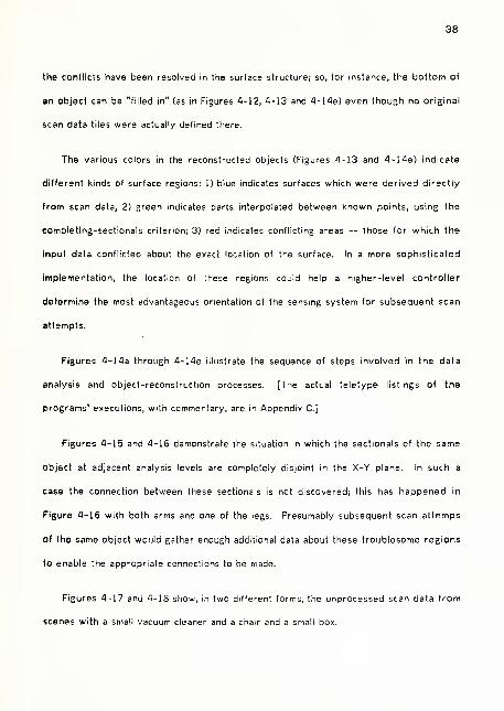
the conflicts have been resolved in the surface structure; so, for instance, the bottom of
an object can be "filled in" (as in Figures 4-12, 4-13 and 4-14e) even though no original
scan data tiles were actually defined there.
The various colors in the reconstructed objects (Figures 4-13 and 4-14e) indicate
different kinds of surface regions: 1) blue indicates surfaces which were derived directly
from scan data, 2) green indicates parts interpolated between known points, using the
completing-sectionals criterion; 3) red indicates conflicting areas — those for which the
input data conflicted about the exact location of the surface. In a more sophisticated
implementation, the location of these regions could help a higher-level controller
determine the most advantageous orientation of the sensing system for subsequent scan
attempts.
Figures 4-14a through 4-14e illustrate the sequence of steps involved in the data
analysis and object-reconstruction processes. [The actual teletype listings of the
programs' executions, with commentary, are in Appendix C]
Figures 4-15 and 4-16 demonstrate the situation in which the sectionals of the same
object at adjacent analysis levels are completely disjoint in the X-Y plane. In such a
case the connection between these sectionals is not discovered; this has happened in
Figure 4-16 with both arms and one of the legs. Presumably subsequent scan attemps
of the same object would gather enough additional data about these troublesome regions
to enable the appropriate connections to be made.
Figures 4-17 and 4-18 show, in two different forms, the unprocessed scan data from
scenes with a small vacuum cleaner and a chair and a small box.

39
Fig. 4-10: Closed contours of object at various analysis levels
%W^^^«i<r-
^^ttiffilFf"^
EWy\l/|^i^v''• T^^
W ^!lS
rlFig. 4-11: Polygonal skin defined over the contours
(different obiect than Fig. 4-10)
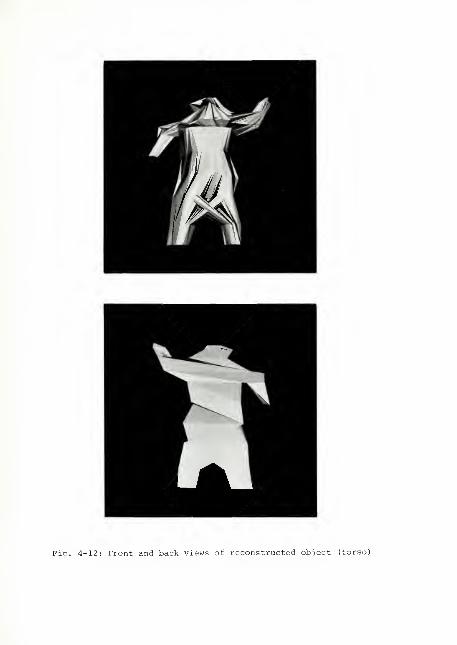
Fig. 4-12: Front and back views of reconstructed object (torso)

[. 4-13: Color-coded front and back views of torso(Blue regions were extracted from the original laser-scan data.Green regions were added by the analysis-reconstruction process.)
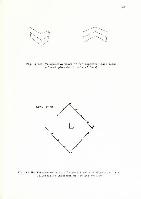
Fig. 4-14a: Perspective views of two separate laser scans
of a sinple cube (simulated data)
zt£<.iEL- 20 eoe
Fig. 4- 14b: Line-segments at a Z- level (from tlie above scan data)
illustrating instances of gap and overlap

43
Fig. 4-14c: Conpleted cross-sections of cube, with aaps andoverlaps resolved
rid. 4-14d: F^-j I'sl-^ective viewsronstiuct^'>d dt
^f sinulatsd cube,and 3 levels

Fig. 4-14e: Color-coded views of reconstructed cube,with and without top
(blue = original data; green = added regions;red = conflict-resolved regions)

45
ZH:^
Fig. 4-15: Completed sectionals at 12 levels
Fig. 4-16: Incomplete reconstruction from the above sectionals

Fig. 4-17: Scanned surface of a vacuum and hose
Fig. 4-18: Laser path ofpath of a scan of a chair and a box
CHAPTER 5
CONCLUSIONS AND POSSIBLE FUTURE DEVELOPMENTS
5.1 Conclusions
A combined hardware and software system has been described and demonstrated.
It can measure surface contours of arbitrary three-dimensional objects and construct
completed closed contour descriptions of all the objects seen from one or more views of
the scene.
While many different methods for acquiring three-dimensional data have been
developed, the present approach was chosen as one which would allow the most
easily-controlled and most flexible interaction with the host computer. The simple,
direct mode of sensor operation -- the digitization of a single arbitrary point in the
system's field of view — seems uniquely well-suited to the general point-by-point,
context-dependent operation of the many pictorial pattern recognition techniques which
seem extendable to the analysis of this kind of three-dimensional data.
Also, if the laser deflection unit and the spinning-disc detectors were mobile, the
system could work in a wide range of environments; in order to acquire a description of
a VW automobile for a computer animation system, for instance, one would no longer
need to manually measure a model VW or the actual automobile; it would be reasonable
to expect that one could simply take the system out to the parking lot ( perhaps only at
night,however ) and have the system itself generate the description. If the system were
mounted on a computer-controlled cart, it might even be able to move around the object,

48
digitizing only tliose parts which the analysis algorithm indicated still needed more data.
As a sensor for a robot, the system may enable more efficient processing of visual
scenes. As previously mentioned, the robot's vision processing could become more
context-dependent; if it just wanted to move through an area, it may only need to
measure and analyze a relatively few points in its direct path. Only when it
encountered an obstacle would it need to digitize the local region more densely, with the
pattern of the points being digitized perhaps being guided by an object recognition
system.
The uses for this kind of system are not limited to traditional computer science
areas. In the field of medicine, the accurate measurement and analysis of the complex,
irregular contours of the human body has the potential for making available entire new
areas of observation to aid the physician in the diagnosis of human ailments. Changes
in the shape, size and volume of various parts — arms, breasts, legs -- may be too small
to be noticed by the unaided eye, but may signal the start of significant physiological
activity. Slowly-developing deformations in growing children may not be noticed until
the disorder has progressed beyond the reach of certain therapies.
Essential to the success of this kind of application is not only a suitably accurate and
practical input device, but also an effective analysis system which can transform the raw
surface measurements into a form meaningful to the physician. The present software
system may be applicable almost without modification to some of these tasks. In the
human measurement studies discussed in [10], some of the forms of graphical output
bear striking resemblance to the cross-sectional contours determined by the present
analysis and object-reconstruction system.

49
The object descriptions produced by this kind of system can also be used to
generate program specifications for numerically-controlled milling machines. A copy of
an object can thus easily be produced without touching the original. This may be useful
either when the original object is too delicate to disturb, or when it is finally to be made
from a material which is unsuited for the design process. With this kind of system the
designer can construct the object from the material of his choice -- clay, soft wood,
plastic — and still have the final object in the required medium, perhaps aluminum or
steel.
5.2 Further Development
Before most of these applications can become a reality, many improvements need to
made, both in the actual hardware sensing system and the analysis and reconstruction
software.
5.2.1 Harware Improvements
The weakest parts of the present sensing system are the spinning-disc detectors
mounted on the corners of the room. As mentioned before, these were developed as
part of an earlier project [6]. While they are an interesting first attempt, they are next
to inadequate by current standards. For starters, a room ringed by four 22-inch slotted
metal discs, spinning at 3600 r.p.m., is not exactly an ideal working environment. The
noise alone prevents all but emergency conversation. More seriously, the heat
generated by the necessarily large electric motors is such that the system must be shut
down for cooling after each 30 mmutos of use. Moreover, the accuracy of the system Is
largely determined by parameters which are difficult to calibrate: the
constantly-changing spinning rate, the slightly different slit positions, the different pulse

50
widths from the light-sensitive Photo-Multiplier tubes.
Another graduate student, Larry Evans, is presently developing alternative digitizing
methods. A number of different approaches are being explored, all based on the idea of
transforming the signals from several two-dimensional images of the scene into
one-dimensional measurements. A key feature of the various methods, the complete
absence of moving parts, is most encouraging. Interested readers are referred to
Evans' research proposal and his forthcoming dissertation [7].
The other major part of the hardware system, the laser deflection mechanism, also
has several serious limitations. Being a moving mechanical device, it encounters
inevitable overshoot problems when attempting to move quickly from one position to
another. The present electronics attempt to minimize this problem by gradually, rather
than instantly, changing the galvanometer signals from an old to a new value. This
solution, however, is a very rough one at best. A significant improvement would be a
system whose galvanometers could provide continuous positional feedback, from which
the electronics could determine a much more accurate control signal, enabling the system
to respond much faster, and presumably with more accuracy. With the increased speed,
more sophisticated sensing strategies -- such a real-time contour tracking — could
become practical.
Perhaps the major inherent problem with the present hardware model is the one of
obstruction. Since it is a triangulating rangefinder, it needs an unobstructed
llne-of-sight from both the laser origin and at least one of the detectors in order to
digitize a surface position. The more extreme the concavities on the object's surface,
the more often this obstruction problem prevents the digitization of a particular position.
One possible solution is to have a different kind of ranging system. One which seems a

51
reasonable candidate is a modulated laser time-ot-flight rangefinder. While there is at
least one such product on the market whose specifications are outstanding, with
accuracy approaching one part in 10**6, its price is unfortunately prohibitively
expensive [9].
Simpler, less expensive systems can, however, be constructed, but they are
presently limited to an accuracy of about one inch [15]. While this is not accurate
enough for most digitizing purposes, it may still be appropriate for certain other
applications like robotics. These would certainly overcome many of the limitations of
triangulating rangefinders. There would no longer be a need for at least two separate
positions from which to triangulate. Thus the operating environment could become less
restrictive. It is reasonable to expect that the range of useful distances could also be
enlarged — for instance, real autos could perhaps be analyzed instead of just toy
models. All these advantages may outway the accuracy limitations for certain
applications.
Of course, for some applications it may be advantages to have either the object or
the sensing device on a movable platform to allow controlled changes of orientation
between the sensing device and the object(s) under consideration.
5.2.2 Improved Analysis and Reconstruction Methods
The range of possible improvements in the software is even larger than In the
hardware sensing system. Due to the modular nature of the software implementation,
improvements in virtually any area can be made without modifying any other section.
The basic digitization could be made significantly more accurate. In the present
implementation, the basic three-dimensional coordinate determination from the sensor

52
input values does not take full advantage of the fact that the line of the laser light in
the room is known. If the deflection system were to be calibrated with some precision,
then the angular deflection parameters could be used in these calculations. A
formulation of the problem optimized to the geometry of the system may also be helpful;
for instance, a polar coordinate representation with origin at the laser deflection point
may yield a simpler set of equations to be solved.
Since the laser deflection is directly under computer control, an obvious
improvement would be to implement a dynamically-changing scan of the environment.
This could be as simple as varying the distance between adjacent sample positions
based on the local surface contour, or it could be as involved as placing the entire
reconstruction and recognition process directly in control of the scan. In this way, the
laser beam could only be moved to those parts of the scene which were of significant
interest to the system.
Perhaps the most far-reaching modification would be to infuse the analysis and
reconstruction process with some 'a prion' knowledge about the objects it is likely to
encounter. Such knowledge could aid not only in guiding the scanning process, but also
in helping to resolve difficulties in reconstructing parts of objects about which there is
incomplete information.
APPENDIX A
MAJOR SOFTWARE MODULES
NWRSL~(NeW Real-time digitization with Scanning Laser) — or RSL — controls the laser
deflection system, acquires raw points from the Burton Box hardware and
software, generates a —.DAT file of all acceptable 3-D measurements in a
laser scan.
NPTDIS ~ (New PoinT DISplay) — displays (onto a Tektronix 4012 storage scope) the
raw 3-D points from a (—.DAT) file from NWRSL . It can also filter out points
which are grossly out of place, the filtering being based on a minimum distance
criterion from adjacent sample points.
NGENPO—(New GENerate POIygonal surface) — reads in a points file (—.DAT) from
NWRSL and generates a surface of triangular polygons over these points.
These polygon definitions are output onto a —.POL file. For diagnostic
purposes, a number of other data files can also be generated. The most
frequently used ones are
—.PTB, a two-dimensional grid of characters showing whether or not
the data point at each position in the scan has been succesfully digitized,
—.MDR, the original data points and the just-defined polygonal surface,
in the standard (MOTION-DATARD) graphics system format. This enables easy
display of the original points and polygonal covering.

54
SCANA ~ (SCan ANAIyzer) — accepts one or more pairs of point (—.DAT) and polygon
(
—
.POL) files from NWRSL and NGENPO; and generates a file of line-segments
(
—
.SGM). These line-segments are the intersections of the polygons with
chosen cutting/analysis planes.
MAKSEC ~ (MAKe Sectionals) — generates a (—.SEC) file of sectionals (closed
cross-sectional regions) from a line-segment file from SCANA.
OBREC ~ (OBject REConstruction) — generates complete object descriptions from a
cross-sectional file (—.SEC) of MAKSEC. These descriptions are in the format
of the current general-purpose graphics software at U. of Utah
(MOTION-DATARD).

APPENDIX B
DATA FILE FORMATS
Original Point File Format
<
—
.DAT file> ::= <scan descriptGr> <a data paint>* [» = one or more instances]
<scan descriptor> ::= <number of positions on a scan line> <number of scan lines>
<scan i.d. nunnber>
<a data point> ::= <pcint i.d. number> <X-value> <Y-value> <Z-value>
A Sample —.DAT File
5 3 1
leeieei +.i 0.01 +201001302 -10 0.02 +101001003 -20 0.031001004 -10 0.02 -10
1001005 +.1 0.01 -20
1002005 +.1 10.01 -20
1002004 -10 10.02 -10
1002003 -20 10.031002002 -10 10.02 +101002001 +.1 10.01 +201003001 +.1 20.01 +201003002 -10 20.02 +101003003 -20 20.031003004 -10 20.02 -10
1003005 +.1 20.01 -20

56
Polygon File Formal
<
—
.POL file>
<a polygon definition>
:- <one text line> <a polygon definition>*
;:= <point i.d. number>*** <carriage-return and line-feed>
[ *«* = 3 or more instances ]
A sample —.POL file
NXSTEPS= 5 NYSTEPS=3 IDSCAN=1
leeisei 1002031 1001002
1081002 1002031 1002002
1001002 1032002 1001003
1001003 1032032 10020031001003 1002033 1001004
1001004 1032033 1002004
1001004 1002004 1031035
1001005 1002004 1002005
1002001 1003001 1002002
1002002 1003001 10330021002002 1003032 10020031002003 1033002 1003003
1002003 1033003 1002004
1002004 1003003 1833004
1002004 1003034 1302035
1002005 1003004 1003005

57
Point-Table Format
<
—
.PTB file>
<one scan line descriptor>
<one scan position descriptor>
<position tias good data>
:; <single text line>
<one scan line descriptor>*
::> <scan line »> = <one scan position descriptor>*
::= <position has good data>
::= <position does NOT tiave good data>
::-X
<position does NOT have good data>
A Sample —.PTB File
NXSTEPS=40 NYSTEPS=30 DSCAN=200000038- X X.XXX.X,,, XXXX23= ,.,,x.,. x XX,,,. XX.. XXXXXX,,,,28- ,,X .,,,x,.x X X, ,XX,,,XX XXXX, ,x.x.
27- X XXX XXX, XX..
X
2G- X XXXX XX, .X. XXX25- x!!!!!!! , XXXX XXX X
24= X XXXX, ,
,
,x >
, , >
<xx
23= XXXXXX, <xx
22= XXXXXX, ,,X XX,
X
21 = X XXXXX. X.,X XXXX,X,,..20= X XXXXXX., XX -—19=..,18=17=
le-15-14-
13-
12-
- .— -,!!!!!!!
- ,
*
; XXXXXXXXXX !!!!.'! XX.
11- !!!!!x!! , XXXXXXXXXX X XX.10- t * * t ( ( t
«
, XXXXXXXXXX XX, ,xxx, .
.
9- XXXXX XXXXXXXXXX XX. XXXX, ,
.
8-,,,,,,,,X. ,.,XXXXXXX XXXXXXXXXX XXXX7- XXX, ,.X, x... ,
6-,.,, XX XX, ,xxxx5- X XX ....XXXX4- X, X , .x.xxxx3- ...xx...2- ..XXXX,,1-

58
Segments File Format
<—.SGM file > ::- <one level's segments>* END
<one level's segments> ::= LEVEL <Z-vaiue> <a segment description>*
<a segment description> ::- <X1 value> <Y1 value> <X2 value> <Y2 value>
<orientation> <a single polygon description>
A Sample —-.SGM File
LEVEL 20.0009. 980 -10.020 000 -20. 000 1002003 1003002 1B33003
000 -20.0B0 -. 030 -19. 970 1002003 1033003 1002004-, 030 -19.970 -10. 000 -10. 000 1002034 1003003 1083004
-9. 980 10.020 000 20. 030 2002003 2003002 2003003000 20.000 030 19. 370 2002303 2003003 2002004030 19.970 IB. 0G0 10. 033 2002304 2003003 2203004
19. 990 .093 10. 000 -10. 000 1002002 1BO3B01 1003002le. 000 -10.003 3. 980 -10. 020 1002002 10B30B2 1BB2003
-IB. 000 -10.003 -10. 023 -9. 330 1002004 1BB3B04 1B320B5-10. 020 -9.930 -20..000 ,100 1002005 1003004 1033005-19.,990 -.489 -10. 000 10.,000 2002002 2303001 2OB3002-18.,000 10.000 -9.,980 10.,023 2002002 2003BB2 200200310.,000 10.000 10.,020 9.,379 2002004 2BB3BB4 200200510.,020 9.979 20.,030 -,,500 2002005 20B3BB4 2BO300520.,000 .100 19,,990 ,030 1002001 1003001 10D2002
-20,,000 -.500 -19,,930 -,,489 2002001 2003001 2002002LEVEL 9.000
8.,979 -11.021 ,000 -20,.000 1001003 1002002 1002093,000 -20.000 -1.,029 -IS.,371 1001003 1002003 1CO1O04
-1.,029 -18.371 -10..000 -10..003 1001004 1002003 1002004-8,.979 11.021 .000 20..003 2001003 2002002 2C020B3
.000 20.000 1..029 18..371 2001003 2002003 20010041,.029 18.371 10.,000 10..003 2001004 2002003 2002004
18..989 -.921 10..000 -10..000 1001002 1002001 100200210..000 -10.000 8..373 -11..021 1031002 1002002 1CO1C03
-10..000 -10.000 -11 .019 -8..971 1001004 1002004 1001005-11..019 -8.971 -20 .000 .100 1001005 1002004 1002005-18..989 .562 -10,.000 10,.000 2031002 2002001 2002002-10..000 10.000 -8,.979 11 .021 2001002 20O2BB2 2001003

59
10.800 10.008 11.019 8.930 1 2001004 2002004 209100511.019 8.930 26.003 -.500 1 2001005 2002004 200200520.000 .100 18.989 -.921 1 1301001 1002001 1001002
LEVEL 3.0002.373 -17.027 .000 -20.033 1 1001003 1002092 1002003.000 -20.000 -7.023 -12.977 1 1001003 1002003 1001004
-7.023 -12.977 -10.000 -10.000 1 1001004 1002003 1092004-2.373 17.027 .000 20.000 1 2001003 2002002 2002003
.000 20.000 7.023 12.377 1 2001003 20Q2B03 20010047.023 12.977 10.000 10.000 i 2001004 2002003 2002004
12.983 -G.987 10.000 -10,330 1 1001302 1002001 100200217.027 1 1001002 1002002 1001003-2.317 1 1001004 1002004 1001005
.100 1 10010E5 1002004 1002805G.8G8 -10.000 10.000 1 2001002 2002001 200200210.000 -2.373 17.027 1 2001002 2002002 200100310.000 17.013 2.G3G 1 2001004 2002004 20010052.G3G 2B.000 -.500 1 2001005 2002004 2002005.100 12.983 -G.387 1 1001001 1802001 1001092
10.000 -10.000 2.973-10.000 -17.013-2.917 -20.003
-10.000-17.013-12.983-10.00010.00017.01320.000
END

60
< —.SEC file>
<one level's sectionals>
<a sectional description>
<line-segment descriptlon>
<type of line-segment>
<standard line-segment>
Sectionals File Format
::= <one level's sectlonals>* END
::= LEVEL <Z-va!u9> <a sectional description>*
::= SECTIONAL <line-segment description>*»«
::= <X-value> <Y-value>
<type of line-seg-nent (from this point to the next) >
::= <standard line-segment>
::= CONFLICT::- BLANK
::= POLYGON <a single polygon description>
<a single polygon description> ::« <point i.d. number>***
A Sample -—.SEC fi'e
LEVEL 20.000SECTIONAL
.000 -20.000 POLYGON-.030 -19.970 POLYGON
-10.000 -10.033 POLYGON-10.020 -9.980 CONFLICT-19.709 -.194 CONFLICT-10.000 10.000 POLYGON-9.980 10.020 POLYGON
.000 20.003 POLYGON
.030 19.970 POLYGON10.000 13.000 POLYGON10.020 9.979 CONFLICT19.709 -.194 CONFLICT10.000 -10.000 POLYGON9.980 -10.020 POLYGON
LEVEL 9.000SECTIONAL-18.989 .5G2 POLYGON-10.000 10.030 POLYGON
1002833 1003003 13020041002034 1003003 10030041002334 1003004 1002005
2302002 2003002 20020032032383 2003032 20030032002003 2003003 20020042002004 2003003 20030042002034 2003004 2002005
1082002 1003002 10020031002003 1003002 1003003
:001002 2002001 2002002:OO1002 2002002 2001003
61
-8. 979- 11. 321 POLYGON000 20. 003 POLYGON
i! 029 IS. 971 POLYGON10. 008 10. 030 POLYGON
11. 019 8. 330 CONFLICT19. 709 -. 19A CONFLICT18. 989 -. 921 POLYGON
18. 000 -10. 033 POLYGON8. 979 -11..321 POLYGON.000 -23. 000 POLYGON
-1.,029 -18..971 POLYGON
-IB.,000 -10..000 POLYGON-11.,019 -8..971 POLYGON-20.,000 .100 BLANK
LEVEL 3.000SECTIONAL-12,,983 G,,8G8 POLYGON-10,,003 13,,000 POLYGON-2,,973 17,,027 POLYGON
.000 20,.000 POLYGON7,,023 12,,977 POLYGON
10,.003 10,.000 POLYGON17,.013 2,.G3B CONFLICT19,.709 -,.194 CONFLICT12,,983 -B,.987 POLYGON10,.000 -10,.000 POLYGON2,.973 -17,.027 POLYGON.000 -23,.030 POLYGOi\)
-7,.023 -12 .977 POLYGON-10 .003 -10 .003 POLYGON-17 .013 -2 .917 POLYGON-20 .000 .IGQ BLANK
END
2001003 2002002 20020032031033 2002333 20010042001004 2002003 20020042001034 2002004 2001005
1001002 1002001 10020021001332 1002002 10010031031003 1002002 10320031301333 1302003 10010041001004 1002033 10020041001034 1002004 10010051001005 1002004 1002005
2031302 20020012001032 23320322001333 20020022031SQ3 20020032001004 203200320E1034 2002004
1331002 10020011001002 10020021001033 10320021301333 10020031031034 10020031001004 1002304
1001035 1002004
200200228018032002003200100420023042801335
10320B2100100310020031001004103200410310051002005

62
A Sample of a Reconstructed Object File
Since this file is in the format of the currently popular Utah graphics software
(MOTION-DATARD), interested readers should refer to the internal Computer Science
Dept. memos on the subject. Basically the file consists of 3-D point positions and
polygons defined over the points. The specific structure of the file here is a sequence
of blocks surrounded by "NAME=" and "END=" statements. The names used with these
statements are LI, L2, L3, etc., indicating the Z-levels at v/hich the reconstruction
process was applied. Defined at each level in this file are the points that lie in that
plane (notice that their Z values are identical) and the polygons that lie entirely in this
plane (the top and bottom "cap" polygons) and the polygons which form the surfsce
between connected sectionals on this level and sectionals on the preceeding level. ( "T"
in the polygon definition sections refer to points at the preceeding level.) "COLTAB"
commands indicate changes in the coloring of the polygons being defined. Colors of the
polygons indicate the nature of the local surface region — being either a 1)
standard-measured surface, or 2) one which was initially blank but was later "filled in",
or 3) one whose exact position was In conflict.
SMOOTH =N0NAME-LlBODY=SCENEPOINTS1182 103 1
4
5 .000 -20.000 -20.000
63
B -.030 -13 .370 -20.000
7 -10.030 - 10.009 -20.000
8 -10.020 -3.380 -:20.000
9 -13.703 - .134 -20.03010 -10.000 10.000 -20.000
11 -9.380 10.020 -20.000
12 .000 20.000 -:20.033
13 .030 13.370 -:20.000
14 10.000 10.000 -20.000
15 10.020 3.373 -20.000
IG 13.703 -.134 -:20.00017 10.000 -10.000 -23.000
18 3.380 - 10.020 -20.000POLYGONS
1 18 5 G 7
COLTAB 3
2 7 8 3 10 11 12 13
AXIS 1 2 4 3
AX IS 2 3 4 1
AXIS 3 1 4 2
END=L1NAnE=L2P0P=L1BODY=SCENEPOINTS1 -18.383 .5G2 -3 .033
2 -10.003 10.000 -3.033
3 •-8.373 11.021 -3.0334 .000 221.003 -3 .003
5 1.023 18.371 -3.000B 10.000 10.003 -3.330
7 11.013 8.330 -3.000
8 13.703 --.194 -3 .003
9 18.383 --.321 -3 .000
IB 10.030 -10.003 -3.000
11 8.373 -11.021 -9.333
12 .000 -2:0.033 -3.003
13 -1.023 -•18.371 -3.33314 -10.000 -10.030 -9.333
15 -11.013 -8.971 -3.333
IG -20.030 .103 -3.030POLYGONS1 tS 8 TG
2 tG 8 ri
3 ^7 8 3
4 t7 3 18
5 t8 3 t3
6 t3 3 10
7 T9 IB tl0
COLTAB G
8 tl0 10 11
14 15 IB 17 18
64
3 tl0 11 12
IB tie 12 til
11 Til 12 13
12 til 13 tl2
13 tl2 13 14
14 T12 14 15
COLTAB 7
15 tl2 15 IG
IB tl2 IG 1
COLTAB G
17 tl2 1 2
18 n2 2 3
19 tl2 3 tl3
20 tl3 3 4
21 tl3 4 tl4
22 tl4 4 5
23 tl4 5 G
COLTAB 9
24 tl4 G tl5
25 tl5 G 7
2G tl5 7 tlG27 TIG 7 tl7
28 tl7 7 8
29 ni 8 tl830 tl8 8 t5
END=L2NAnE=L;!
P0P=L2BODY=SCENEPOINTS1 -12.383 G.8G8 -3.0002 -10.000 10.000 -3.3303 -2.973 17.027 -3.0304 .00E1 20.000 -3.0005 7.023 12.377 -3.030G 10.000 10.000 -3.0307 17.013 2.G3G -3.030
8 19.709 -.134 -3.033
9 12.983 -G.387 -3.03010 10. 000 -10.000 -3.00011 2.973 -17.027 -3.00012 .000 -:20.000 -3.00013 -7.E123 -12.377 -3.00014 -10. 000 -10.000 -3.00015 -17. 013 -2.317 -3.000
IG -20. 000 .100 -3.000POLYGONSCOLTAB 7
1 Tl IG 1
COLTAB G
2 tl 1 2
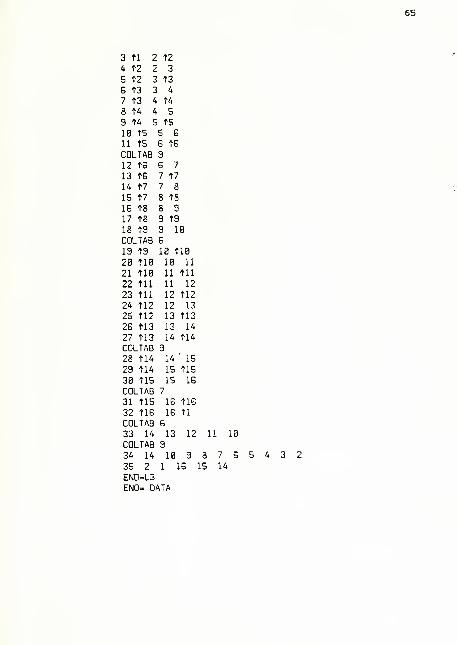
65
3 tl 2 t2
4 t2 2 3
5 t2 3 t3
G t3 3 4
7 t3 4 n8 t4 4 5
9 t4 5 t5
10 TS 5 G
11 t5 G TG
COLTAB 3
12 TG G 7
13 tG 7 ^7
14 t7 7 8
15 t7 8 t8
IG t8 8 3
17 tS 3 tS
18 T3 3 18
COLTAB G
13 t3 10 tie
28 tia IB U21 tia 11 til
22 til 11 12
23 til 12 tl2
24 tl2 12 13
25 tl2 13 tl3
2G tl3 13 14
27 tl3 14 tl4
COLTAB 3
28 tl4 14 15
23 tl4 15 tl5
30 tl5 15 IG
COLTAB 7
31 tl5 IG tlS
32 tlG IG tl
COLTAB G
33 14 13 12 11. 10
COLTAB 3
34 14 18 3 S 7 G
35 2 1 IG 15 14
END=L3END- DATA
5 4 3 2
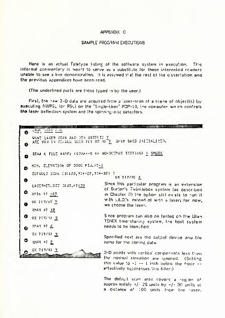
APPENDIX C
SAMPLE PROGRAM EXECUTIONS
Here is an actual Teletype listing of the software system in execution. Thisinformal commentary is meant to serve as a substitute for those interested readersunable to see a live demonstration. It is assumed that the rest of the dissertation andthe previous appendices have been read.
(The underlined parts are those typed in by the user.)
First, the raw 3-D data are acquired from a laser-scan of a scene of object(s) byexecuting NWRSL (or RSL) on the "Single-User" PDP-10, the computer which controls
the laser deflection system and the spinning-disc detectors.
WANT LASER SCAN AND 1)TA OUTPUT? XARE YOU 0\ 3l;:GLE USER 7CY OR N) Y_ GP13 DACS INI TIALI rEI).
DTA# 4 FILE NAME; (DTA^«-8 z> NO-OUTPUT TESTING)J_
5MD0X
niN. ELEVATION OF GOOD PTS,-7M_
DEFAULT SCAN ( D: 1 OB, X:+-2S, Y:+-30) 7
LASER-0'3JECT DIST.r7ir.3
XNIN -? -25
OK 7(Y/N)' Y.
XMAX :?_1J_
OK 7(Y/N) _N_
Xr-'AX :? ^OK 7(Y/N)
Ji_
XriAX :? 2.
OK 7(Y/N) Y
OK 7(Y/N) £Since this particular program is an extensionof Burton's Twinklebox system (as describedin Chapter 3) the option still exists to run it
with L.E.D.'s instead of with a laser; for now,we choose the laser.
Since program can also be tested on the UtahTENEX time-sharing system, the host systemneeds to be identified.
Specified next are the output device and file
name for the coming data.
3-D points with vertical components less thanthe minimal elevation are ignored. (Settingthis value to -1 -- 1 inch below the floor --
effectively suppresses this filter.)
The default scan area covers a region of
approximately +/- 28 units by +/- 30 units at
a distance of 100 units from the laser.
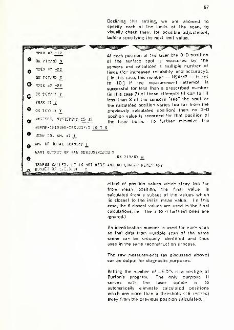
67
WIN :? -IB
tt OK 7(Y/N) _N_
G Y!1IfI :? ;23_
OK ?(Y/H) _N_
YtllfJ :? -26
e OK ?{Y/N) Y
YMAX =7 a.
e OK ?<Y/tl) Y
o NXSTEPS, NY3TE
NSftMP»:i1INSflr!»
9 SCAN ID. m. -
PS:? 15 15
:NCUT0F:7 10 7 6
Declining this setting, we are allowed to
specify each of the limits of the scan, to
visually check them, for possible adjustment,
before specifying the next limit value.
At each position of the laser the 3-D position
of the surface spot is measured by the
sensors and calculated a multiple number of
times (for increased reliability and accuracy).
[ In this case, this number — NSAMP -- is set
to 10.] If the measurement attempt is
successful for less than a prescribed number
(in this case 7) of these attempts (it can fail if
less than 3 of the sensors "see" the spot or
the calculated position varies too far from the
previously calculated position) then no 3-D
position value is recorded for that position of
the laser beam. To further minimize the
NM. OF TOTAL SCAHS:7J_
WANT OUTPUT 07 RAW f^ASUI^EMCNTS 7
OK 7(Y/NJ Jl
TRAPSS CALLED. IT IS NOT HERE AND NO LONGER NECESSARYnu;i3ER of L. E.D.3: 3,
itiMrTTTiiiiirifcBrtiinirfflfciiJTiTTrfc tm» ami ?]%> ritkMidBHi
effect of position values which stray too far
from mean position, the final value is
calculated from a subset of the values which
lie closest to the initial mean value. (In this
case, the 6 closest values are used in the final
calculations, i.e. the 1 to 4 farthest ones are
ignored.)
An identification number is used for each scan
so that data from multiple scan of the samescene can be uniquely identified and thus
used in the same reconstruction process.
The raw measurements (as discussed above)
can be output for diagnostic purposes.
Setting the number of L.E.D.'s is a vestige of
Burton's program. The only purpose it
serves with the laser option is to
automatically eliminate calculated positions
which are more than a threshold (15 inches)
away fromi the previous position calculated.

68
In addition to going onto the DECtape, thedata can also be directed to another device; in
this application, output to the Tektronic 611storage scope is the most convenient,enabling easy monitoring of the scan'sprogress.
f^^gr"^^ w
(Scale factor for putting data points onto the
scope.)
DATA TO TELETYPE, SCOPE, OR DISX CT, S, D): ^SCALE: _1_S.
SI NGLE OR QUADRANT: Q_
GO? _r_
E>JDFILE A'JD CALL "ELEA-B O'l 1 Pi
Nil. OF 3AD POSITI 0N3: 37
DTA* * FILE NAME; (OTA*<-!' -> •JH-O'ITPUT TESTI'.'n) tC
o —Quadrant option puts the data onto the scopein three different axes — XY, YZ, and IX.
(The scan now takes place — approx. 5-10minutes.) The End-of-File written onto
theDECtape file signals the completion of the
scan.
The number of points rejected (as describedabove) out of the (40 x 40 =) 1600 total laser
positions.
Another, new scan can now be specified.

69
-SCOP TSIXI .-1
5 i 1
AT: '' CT1) TTY; f 3" 1
la^lfi?! +.1 1 ."1 +211C>(^1?|?2 -1" 1.1? + 13[(^'^l'^'^i -2? -.13 1
l'?<»lfl''i -i" 1.12 -I?l(ni^T5 + .1 1.11 -21
1 •n2^'^5 + .1 1^.11 -211112"'"^ -M i;i.?? -11in-i27nj -?^. 11,13 n
1(1'12'^^£ -IT n."? + 11
10?2^'^1 +.i 11.11 + 21l{n3<l^l +.1 ?"."! +2
1
i^ij?"^? -n 2 1 .1?. + 11ll^3fn3 -2 1 21,1,' 1
imjna -i" 2 1 ,'^2 -11ir-r.SiT? + .1 21,11 -2 1
iC:)? Thai's ."^5Tr ^ (TO) TTY; f I''1
5 3 22'!i^i:i''l -.5 1.11 -2 I'
2'T^l :i'T? +1 T 1 12 -1"
2'^!in?!3 +21 -« "3 1
2'^'71 11^^ +11 1 "2 + 11aiTl I'^'i -.5 1 "1 + 2 1
2?l2cn5 -.5 1^ "1 +2"2T7i?17il + 1 T 11 "? + 1"
2112 ^l"? +?" 11 13 1
2 112 1-2 +1" 11 "2 -1 '•
>ii2iill -.5 1" 1
1
-2 "
insiii -.5 21 "1 -2 1
2ir>3iiP +1? 2 ^ -.0 -112113715 +21 21 "3 1
21?3iiJ + 11 21 1? + 1"
2^i3n'>'S -.5 21 "1 + 21•?N3F-;pi
1 MP'JT FILEtTTOif 1 .: ;t
WANT POUYTHM 3-0^ILY TLF?"NEW POLYG.I'J filh: •ja:'1F=^t='i^i .^y.
WftNT M1-301D P1I.VT I'l? ' FI '_F?'f
WA^JT POI MT-TATL?: "^ILF?186S -)3K PA- FT UFF F! !
FUCH3 13 31 S
2PA"FS OVF"? ALL^^^ATITj
WAMT IITI OM- lATA^ri .1IITPMT7V
10TION-->iTA'7l r i_f' -T^S^T^" 1V1 . 'i^
VA^IT Ft L'. -3 LA 'K-P II 'JTT ^^
•JX3TEP?;5 'JVTTF°3r3 I1";CANirEMTE" LT'IT"- TF '.'1"vlM'! '/-^''i'
.|i:i 111 -111 ii'< -1 '^i1-1
Listed now are the original data files, as they
would come from the digitizing software
(NWRSL). As described more fully in
Appendix B, these files start with a descriptor
line, telling the number of samples on a scan
line (5), the number of scan lines (3), and the
scan identification number (1 or 2 here). Of
course most actual scans contain several
hundred points or more.
It should be noted that the data used here is
simulated, generated to illustrate, with minimumdistractions, much of the system's capabilities.
We first generate a skin of polygons
(triangles, actually) over all adjacent points
which are in the input file.
N -- We don't care to save (m some disk file)
all those polygons which are no good — those
for which one or more defining points are
missing. We know that all current points are
good.
POINT-TABLE -- is a scan grid showing
present/missing status of each point.
(Like some real-world creditors, this computer
system mercilessly pesters over-extended
clients.)
(Dashed lines indicate typing errors.)
TBOXl.MDR —This will be a point and polygon
file of the just-defined surface in the format
of the currently standard graphics software
at Utah (MOTION-DATARD).
EITER BITTH''SwDOTH^Nn>JArE::$CA^)
niJi^T HFinHT CF09 CiLl^IN': 'R^l
All points NOT within this defined volume are
assumed to be incorrect and are discarded.

70
The rest of this program is diagnostic messages!
a +0 ("CONTROL-0") disables this kind of output.
We now look at tho polygon file just goneratod;
it looks good " just a list of input data points
which define each polygon.
The large point i.d. numbers make it
particularly easy to integrate data from manydifferent scans into the same analysis structure
and still maintain unique point i.d.'s.
We now look at the standard graphics format
file just generated. It contains, in addition to
the aata in the previous point and polygon files,
a definition of orthonormal vectors for easyrotation manipulations when later viewing this
object. This file also defines two additional
polygons — a "floor" and a "tab" on this floor —to aid visual orientation when displaying the
object(s).
EXIT.tC•SCOP jaoYi .poi.rj (TO) TTY;NXSTEP3 -5 -Jr^TEP- r3 I'r;CA')t
l'^'^\c''\ lo'ij-ni 111112IdCTlfl;^? iinj-i^i 113112I0iii'i2 le'^^^^^ 1111-3isiai ^^i \'•?2'^^2 1'"2113
l^dimi Mri2Ti,1 111 114l?.^la'^A 111211? 1121-14
fillip inri^d -''1''15
1 111 115 iTisnj ''IPTI'i
ITa?-! lii^"-"! -121"'?
n-12712 l'n;i"i -i3''->2
1'3'2:'''2 m3Ti2 - 12 113lfl?2'Jn3 H'ljT'? -T5.115
lfl?2 7.13 l'"13^-'? -12114IT:^2^?i 111?:""? 1-^-1:1
\'^n2'•'i I?ij^ia 1-2115
1 :n2n"15 1 --"Jn-i ->3ii=;
^COP T^ovi .•n^.'^ cn) TTY-SMOOTHr'J-)4Avf::,Ci'Jl
301-f-3Zf\lP0I-JT3
I 1112 1 1 T
3 -^ 1 1
4 1 1 ^
5 -31 -5 ?5S ^5 -S 257 ^5 -5 -J?!
8 -31 -5 -3"«> -31 5-33POLY'^nvnC0LTA3 ^
1 5 6 7?2 7 R Q
3 c 7
AXIS 1 2 4 3AXi; 2 3 4 1
ATI- 3 14 2
'ND-SCA^ltJA^.F:-"')'-;!
go)Yr';:f:^JF
POP-JCA'JlPnpJTS1 .in .'111 21 .-- 1
2 -l^.Ti^ .'"O n.i-i3 -21. Ti" .1^ 1 . 1 " -
4 -l"."-!-" .1? - -l-.-'l5 .111 .111*; .1'"' l^.ll 1 -2 1 .1 117 -11."""'' 11. '2 - - 1
- .1
1
? -2-. 111 1".Q -11,111 IT. 1-.--11 .in i^." 21.11-11 .111 21.^ - 2 " .-11
12 -i'.^-"-" r^ -.0 •.1 - -
13 -2 1. "'"' ?^ !->- .-I'"
14 -i^.ni 21 .121 -11.115 .l-^i ?i.'i 1 -21.-11PnLYoO'^l^
1 1 11 2
The point values here match those of the
original input files, except this graphic systemrequires consecutive point i.d.'s, starting with 1.

71
3 2 Q J
4 3 ? S
5 3 ? 4
6 4 8 7
7 4 7 5
8 5 7 6
9 M 11 Q
1'^ 9 11 12
11 9 12 8
12 8 12 13
13 8 13 7
14 7 13 1415 7 14 ^
16 6 14 15EN:)r30'<lENOrDATA9NGE^J='}
INPUT FILE: Taox2 .lAT
We generate the polygons file for the second
original point file. (Exactly the same as for the
first file.)
WANT P0LYG1-!?-0-JLY HIE?1 837 rr3K PAGE" LE"T! !
F'lCH^ I? 31 7 ^Af^ES OVE^ Ai.LXATIOMMY_"JEV POLYT'TJ '='ILE \|Af1E-?TS2][^_^P2L
WANT ST -GO 10 POlYGTl" ' FILE?!
WAMT Pni'lT-TA3LE nLE?S
WANT roll i"J-riATion TilT=iiT7v
>IOTn'J-^ATA=^ FILE:?T? 1^2 .-T^
WANT FI i.L-SL'i^K -PII "IT^ ?N
•)XSTE'==;:5 NV^TE,='~-3 n^C A JrJ'-""'•-
ENTE« LI"'1IT~ -I- idop/pi:; '.nMi^r. ymj'j v-^v /•[.. v-^v -..,.. ....^y ->.
-l?Pi IT- -l"n l"!" -1"" 11^.....
ENTEP '3 07X1" 1=' 1'3JECT' HEIGWT ("op criLl'l'i-; -rf, i-^.
S101T" -'lO
•JA^E:3CANYN3V I'JITIALITET T1 1 PTn.^EXTO~
For experimentation, let's alter the value of one
EXIT.g, ^l^g original points - from -.5 to -87.5.
•SPTET
°OET .3 -TEC -74 T'^o
#rea:) T^i'^g.iAT ; V -1 'f^psi^'j)
*£1.">IT
20.:iI?->I -.5 ^.-i -?T23^1 mi -<g7.5 i.iii .??
2?11'?T1 -"7.5 T."! -2T* 1 .5/5 3 2
2''Ti:'.il -37.=. 1. 11 -2T2C?'^1 (i:>2 + n T .nj -l i
21tll TTJ 4-?'' "^ .^? "^
jovEP^'PiTE T=^nvo.i.;.7 fjrn vc-.^io.! ^^.^ ^^^^^ ^^^^^5^ ^GENPO to get a polygon
•aNG^MPA mapping for this altered data file.
I NPMT FILE:T?2I?_^^1AI

72
WANT POLYm^s-TJiv^HLE? We'll now look at a "no good" polygons file
FUCH-^ls iac^^PAGErovEP ALLo: ATI d'j ! !*° ^^^'^^ '' **^^ polygon depending on this
Y_ altered (and to be discarded) data point is
JEW POLYGO-j FILE NA i-;?T 'A vo'^? .^T- also discarded.
yANT NT-'300a PILVTTJ- ' "ILF7V•JEiV 'FAILEO ' PILYTO'J-; ' FILE 'ii\''.--^l'r-)r2.-r,^
WANT POI'JT'TA^L^ "T'^'^y
POlNT-TAgi E Fii Et?T91''j'.pt'>^®'" ®'^° '^^'^ ^* —.PTB file and check for
WANT •lOTinM-DAT'iPD 0'IT^'JT?YMOTIO'J-OATA^D nLE-?Taovr .-il'^
the discarded position.
Hopefully by defining the acceptable
WA "IT FILL-BIA'K -PipjTS ';J_ volume, the previously altered point will bejudged unacceptable.
'JXSTE?$r5 'JVSTE^^T^ I I'^C am;? ->?ii^i
E'JTE'^ LI "I T? IF VT'-rl-JT VOLU'''!^; Y-I'IYMAY yvrvv-^^v -^r., ,«,v ,.
-2 5 ?5 -rs rs -rs 25' ...
ENTEP 'BOTTnv 07 ;1^,ir:;T ' iiri -;uT cn^ -OI^O^I-JT '>:;ri -,--
9f^ioTM-'n ~NAKE^CAvY'jov ruTiALnn ti 1 t'lnto
jvij^ As expected the discarded polygontC definition appears in this "discarded" list
^:o= T?Oxg.^r,? H an) TTv. fOK!(it's the Only entry).
aji'i"?! j-rijiii s^-ii-Ti?-sens Tmy?.PT^ ;g (to) ttyj
( Tf 1 Looking at the point-table file we see (by
3-YyxyV^''''''^"^'-^ n-ciM-?-^-^'---
the X's) that most of the positonc have
gryxKKx valid entries. The only missing positionl^.xxxx (markded by a ",") is the first sample in the— first row of the scan — the very point we
Xij'^vY i*:3TF? CY/'j)-j severely altered.
pnpjT FILE 1 =T?T'l .1AT
:)E3Ci^IPTin-J: 5 71
TOTAl. "i". PT5 . : 1 "i
UA'JT 5 01TE1 .' 01 MT9 - CY /))'.'
P ILY 'O'J FILE 1 ^TBTXl .^OL
SCANA - This will accept an arbitrary
number of point and polygon files and
generate the line-segment intersections
between positions of the cut-plane
(analysis plane) and the data polygons.
HE^CIPTI VJ; '0''=:TE=7-? MVCITrn-;-^ It:^-;.!;,.
TYPE 1I-;CA'?TtT POLYTHJ^? CY/"))^
lAX.^RTU'J"! -LEVEL?I 7A5 19" =AT"- LE"T! i
F'lCM" 15 3?A PA?f- iVf'^ iLL'^CATn^J! r
TOT'^L "" , P IL'''^ n'j; -1;
TOTAL 'f . P0L*'C5T\S CTM^I 1'^'^'^-
POpiT FILE prT'^iYCi ,-iiT
lE^C'I'TI V:'r 'S ^
TOTA' ')'. P T? .: J""
WAMT SmTElt TI 'IV,> (Y/'D^^
( 1):I 11^ |1C1 PT.CI-l
One diagnostic output is listed here — theoriginal points (from all input files) sortedby their l.d. numbers.

73
t <o
C
C
c
o
"C ~ ^-^>z I'/I'M '/l/ii- 1 l.'VI'l -1 '1 ..V/IM •iy M
( 3): 1 till Cl'^3 ,1^1 -? 1 .111 "31( 4): n;^ni4 -l^/lil -1 1 .ll'-" 1?CI
( 5): l^iTn-'s -21 .111 .111 1|1< 6)r \''|^2n^\ 21 .nil .11" i" 11"< It- \n'\2'"^2 1 1 .1" 1 -1".11" 1" lO/l
< 8): 1 ai^2CT<i3 .111 -?" .dll 1" "' 1
{ 9): 1 T"2314 -i-p.m -1 1 .111 11 "9 "
( l(!)r 1 T1prn5 -21 .'»i 1 .11" 1" "1"( ll)r l'^13^''l 2i.1-'i .111 21 "11( 12): 1 (113112 1 1 .I'''! -11.C111 2" "2 1
( 13): \?l-^i'"^l .I^l -21 .nil 21 131( 14): 1 IIJCl 1^ -ll.1"'1 -1" .11" 2 " ion
( 15): 1113115 -2 " .111 .1 CI 2" "1"( IS): cimi -21 .11" -"7.51" "! "
C 17): 2111 1"? -11.11-" 1 -.111 "21( 1*?): 2111113 .111 2" .i"i "^"
( 19): 2311"'i^ 1 -."ll 11.111 -»o 1
( 2^): 2111115 2"-" .1'"i - .=;n "1
1
( 21): 2?l2i''l .01 ^^^.1 -.511 1" "11C 22): 2112112 1 " .111 1" "21{ 23): 2113113 ."11 2" ."11 1" "^1
{ 24): 21^21'^1 1 ,111 1
" .""" 1" "2 "
( 2 5): 2 CI 512 115 2 1 .I'l - ,511 1" 1 n
C 2 6): 2^13111 -2 1 ,"11 -.511 C 1 "11C 2 7): 211J119 -11.-11 I". 11'' „ "2 1
( 2P) : 2'"'3i'^3 .11
1
2 " .111 ?-" -.7 />
< ?9): 21131"^ ll.l"! 1" ."1" 9" •"9 ->
< ?T): 2113 """t 21.11" - .SI1 2" "1 1
PT.Y3o^) filf: 2:T^1X2 ?1i.
DE-CflPTI VJ 'jyjTrs- 5 -jvcixr; ?-' n^c 1 ^J -2 1 1 1
TYPE ^nCA^I'O D-i_v- 'IJ--' (V/M)
1 723 OSK PA •~F.- i.^-T !
FiJCHs r; JC J PALLET OVE^ ALLXATI O^J! '
X
:iAX.3f(0'JMO-i.EVEL?/M_5_
TOTAL •!'«. P"!LY1;v;?r 31TOTAL 'J". pnLYQVJ- CONJ?! Dr^-,"):
POINT FILE 3:
TYPEOUT PJI 'JTS ? CY /•»_;]_
TYPEOMT P-IL^'O'-I- "! CY/M)')
TYPEO'JT HI7I i LO-J ' '3 ? (Y/-))>J
TYP^OUT SORTEO ~ ? CV/>i)^
1 21.13" " 131 19
2 21.131 a -.9 1 13
3 21.13" " "2 1! 4
4 21 .131 1 ij" 2 7
5 21.131 " ,V-> r.2 '
6 21.131 1 12 " 2'>
7 21 .12 1 1 19 1 11
? 21 ,"2 1 1 "2 1 1 1
9 2i!"2i 1 "1 "1 5
n 21 .121 1 "1 1 1 S11 21.121 1 2S1? 2 ".121 1 "2 " 2 "^
13 211 .12 1 1 11 " 3114 21 ,"21 " 11 1 3!
15 21 .11 1 1 111 9
Another example of diagnostic output —
the high and low 1 values in each polygon
- sorted by the high Z value. (This is
useful for determining which polygons
intersect with a cutting-analysis plane at a
given Z level.
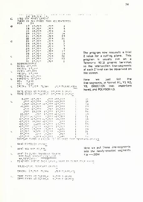
74
I fi 21.11 (" 111 722 DSK ^A^ET LFf^ T!FUCH? 13 ?2 4 PAGE=; nuE^ ALlocATinV^\<^ 2d
1 7 151 .(131 .131 ^
18 l!'.:i5i .131 5
19 in.?3i .121 f,
?n 11.''31 .131 1021 11.13.1 ,121 2122 ICI.131I .121 2!
23 1 1 .121 .121 22« 11 .12^ .121 325 11.121 .11 1 7
2S 11.121 .111 g27 11."21 .121 172? 1 1 .1? 1 "2" IR29 H.'^S" "1 ? 2?.
3^ 1 1 ."2 1 "1" ?531 11."11 .11 1 1
SCOPEFACm^:XLOVr -2" ,'""'
X"IGWr ? ",?''
YLT'^'- -? .5^1YHIGMt 2 -, ^-mifO?I?IM- 51? ."11
YORnplr ^31.'^3^
yc= 7.1S3YCr 7.15?Z M I jW - ? ".151 ''L TJ .11 " 7'."^
TY°E EDIF q AT ''l^v -1 2" _a-,n, , jv
TYPE E33: q AT 'i.EV =:l ?" !"ii ? c
9 ,o<?i -1"."2^ r,^^ .o-" ."
'
.CT-n -2c« ."n . 'Jl -"ic 07"-.13'" -1? .'^7" - " "11 -1
"
T-x..
-fS.QS^ 11."?" T-17 -.-.1
.(^.Tl 21. ""1 "3 ' 1^ 07
.dJCI 19 .9 71 1 111 11 /..r,,.
1? .QQT .IQI 1 1 1 -I" -, , 1
1-'.'"' ,-1 1. •''• ^T' -1
"
T-) ^
-1 1 ,TT7 -11. -n - " 1? " -Q ::t;i
-1 T.??T -T.qc;.-' .OT 1 ' ^ 1"'-!?.<:?" -.J'^c . 1 "'••
'.
1 1-> 1 .
-l".^"^^ 1'."^' -1 3
" 1" -..- •.
1 1 .111 11." »" 1 "•? 1 c:7'3
1?.'?" Q.CT'-- ?•" TT" - sn
S"."^! .1"" = go -• 1Q 1
.jn _-i n -.5"'" - ^ 00 -. - ^O'^
DI-^'.AV ^ ll'Fi ? ( N) 17^ ; 'F' T" ^VI
The program now requests a trial
Z value for a cutting plane. This
program is usually run on a
Tektronix ^012 graphic terminal;
so the intersection line-segments
at each Z level can be observed on
the screen.
Here we just list the
line-segments, in format XI, Yl X2,
Y2, DIRECTION (not important
here), and POLYGON l.D.
WAMT S3 -in IE? (//.') /
U4>JT "JE'J =:^'~' "!L^?v_
VAMT n CLIt'^ '^viqxi'.'T "I'.E?V
Fiviquc-) T'iT="iT T'-JI' 1.'^'."^'.. v'AVT 11 ~i
TMIGHt 21, "31 ^Liu- .111 'i_r\;ri_-
TYPE ET^=:- -T "'LFV'^'.r o.ii" > (Y/'MXY^E E'l'-E'^ AT 7L'"Vri_- =.111 ? CY/'JV
Here we put these line-segments
into the newly-created segments
file —.SGM.

75
DISPLAY EOGES 7 (NnTE!:
WA'JT "G-iFILE? (Y/N)Y
E n EXIT RT* DI3Pt.4Y) CY/'HS
WANT NTJ ?'31 FILF.?2
flMnuE-i TITPIJT THIS LEVEL. 'M*!! TO CLTSE T LE N'D'J?^
•^LP.TI -LEVEL DI"PLAY? (v/^!)•J
AT 7LEVELrAT 7 LEVEL
-
."^1 '^ ZLEVEL:?3
J .""T ? (V /y>
0I7^i_iv r)STS ? f -nTE;1 -i?? "IS" 3i^ES L'^FT! !
FIJCWS IS 3£/- =Ar,FS OVE'' ALLI'ATITJ
rti^c? (v/.))v
Tfi Fi'IT "1^ 'DISPLAY) fV/'nv|
I A "T NE'J SS-1 Fl i_r?2•iV.cjEqur-.'XSr !<;
"I ;iSi-T"i T'lT^'IT T"IS '. JA'IT T" CLIS
'•1"LTI -L^VfL 0[-:^'_AV tv /'!)":
^CT' TSVlf .'-S-T 1 Cn5 TT''r~n'< 1
LEVEL
-2^
LEVE
1
I''
1 1
-1 1
-1 1
-l«
1'
11
21LEVEL
? 73 - 1
7
TO?
"^1 -0''"'
1T
Q 79 J"
5-n -10
-,niT -1
071 -IT72 1
IT!! 1
071 ic02 1 n"•11 -1171 -? 1
=,S? -I''
I11 1 a
12 7
"11 -?117-1 -r-111 -1"1-1''3-' !<=
-. T-II
"
ni -1 "
051 -1"
Q 70"10111OOQ
10 1- J9Q
-?" ^11
-l-^ 571-11 -11101 1111° 071
0711 11
After selecting several other
levels for the cutting-analysis
plane, we close the .SGMfile.
7v_
We next list the —-SGM file
we've just created. It not only
gives the definition of each
line-segment at each level, but
it also preserves the definition
' of the polygon v/hich generated
Ithis line-segment. Although
r this information is not used in
' the present im.plementation, a
Imore sophisticated one could
- take advantage of this
" (line-segment to original
1 polygon) mapping to control the
- explosive growth of tho number^ of new polygons generated in
''
the later object-reconstruction
1 section.
"Ill11^1-
|iil'
• 11? 1-
J
"J 1 "12-1
J
••2 2'''"2'T'3
13 2""! '--'A
13 ^•f2^'^^-1 ll-oi^j'"2 1 11] "iij
"J 1-11 7151/1 11121-s
2'^i2T'2211] 1132 11] 115
'•1 l-""l-'i2
lllj ,,^,,,^ |T^j>^,j
1'"'31 1-2^13 1111114

76
-1."^^ -Vi .TT? -i ^ T^'. -11."11 1
-2.5 7J 17.12 7 TT^ 2'^.7i?.7' 1
."•?' 2^.''-''l 7 1? J 12.T77 1
7.i?3 12.977 M 1? •^
1 1 .111 1
ir.'--'^? -<.'^''7 l'^ T"1 -11.111 1
l'^.^:i^ -n.^i^ 97? -17.1? 7 1
-n.T7T -If .".Tl -1 7 113 -?.'^17 1
-1 7.? 13 -2.^1 7 -i^ 711 .ii;'
1 <2< o-K Pi^-iF- LFFT! !
1 i:'ll-^l5 I'TiTT'^^lIC'^ " 13 3?^ P'ASF?h \'r^'\2'?,^',
-12.ass 'S.'^<^ -IT.'!""!-' 11. 1(1" 1
-i-i.ii'j! I'll. 7^- -r .07? 17.12 7 1
I'."'"' l^'.-'^T 17.?1J 2.^< 1
i7.'^i^ r.^v": ^'.-T' -.i^l 1
21."11 .1?!^ 1? .QS'J -6,9!'7 1
"^ •»! a< •; FC
ll^in/i I'-id^i^ 1119114pill"?? p-Jrip^ir^p ?119115
2iiin/) 2ii?ii? piip^i^l''l!'"''? iT-pi"! 111?-"!?1111119 1119m? in|iii;1 111 i''4 1119114 IdillTi
9111119 9'"'911I Pllpl"?p 'Timp pT,-,p^„p paT|iq^fllH/l ?'"'9'>14 911111Spnir,^.; p/np-,^^ p^qp^^,^
1 111 ""l 1 112111 1 111 119
'.'i'!T T.) 41.1.'^ Y3 CA'.l CTNN'':T7V
We now call the program which
organizes the simple line-segments
into closed contours (sectionals) at
each Z level. (Much diagnostics
follow.)
^', : V : ."1 1 t; J
<L?'V"L> <9 .ooi>«*<! 1.11 i> *-l "
.
**i> <2 -1 ^-./^-i , ^
I?ET- 1
1TI F- -2 .111T 1_ r v - 2 f.n'" Tia
•-DIF- -2 .11"^-iir- 9 ."("'
niFr - .J.i?
roiFr 1 .9 52ni ?-. -1 .9!15
'ni?-- ,.1^?>13I- = -r.915•^-)IF- - .il'^
v-)IFr -1 .913•;F.V4I2r 1 7
')EU3I2: -1?SI'E'S: 5
LOOK 12: 7
AI5E^r s
LOOK 12 r 11MIIFt 1 .001•Olfr 1 .9 52
ISF'^:fDIFr 1 .OS""^DI -r 1 .0 19
>JEViI2r -19•lt'J3I?r 214I5?:nr 7
LOlf I2z R
SnrTr 11'.01KI?r 1 1
IDIFr 1 ."00
"^^I 'z -."PI'-DIFr - .10 1
I5t?r 1
1
iniFr -.111n^IFr -1 .99:1
rDIFr -2 .111
'> <LFVfi^
<:-0 .'
10. o<;
1 t'
-1".el O .00'
TPYI 'JTf^~FCTI 1M; I'JT'F'':
More diagnostics (solely
system designer's benefit)
for the
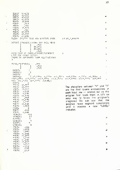
77
TJl r- -1 .yiv
m\?-. -1 .99(1MDITr -2 ,'^'^n
101 7- -1 .9-^9
*IDIF: 2 .ci:^'^
•"OIF. .-sn;oi ?-- .191'niT-- 2 .-^^l
'n\?-. ,TQ1iniFr -7 .-TiZ^
•O: Fr -2 ,"l'^'^
•ni Fr -I .919LE:Vr 2n.T>'r 1IA3 AT: SWaPPFO !=;£ 1 « fV ) * 111'^
'jFF0=f CTJ'JECTLF'J^TH; TIP TAIL 9!<^T
1 1 .1M1 2 >^9 .<1Q 4
2 1 JQ.OQi2 ? .113
'MMT '^lAC AT F'JTF.'-CTJTI^^TLFM'^Tl'?1
^"'3 i;^'< °'^j!i!'; L^"T!!-'ICW3 I? 52'SPATr3 OV^o ^Ll ^C A TI T) ! !
J
; \'Ai.-"I 'JTlTA'.r ."291 1 .11 "
2 ' .11 5
lATI^; 1
lATAI'.t 1
TATI"; 2
lATML- ? < ^ . '> 70 >
+ 1-7.950 > ^li.-"-. <-\*> <I 1
.^lo, <2"'.iii.
i-?;'^r 1
'">I F: -2 ,ni«:)!Fr -2 .'^Tl
OIFt 2 .I"""!
101 f- - .I/I0
"niF: 1 .9 '52
^DIFr -1 .015•^01 Fz .14R•'^I f; -1 ,ci5•'11 Ft -.''"" 1
"IDIFt -1 .= 43vOIFi -.USi-^zr-.-- ?niFr .ti3«
-IIF- 1 .<3 43•I!;wai2r -1 S
M^'ei2r 17/il'FGr 7
LOOK 12 t 7
3I5E3: Q
1. 1 HK 1 2 r S
•91 Fr .C^33vr>lF- -.Clfll^
IDIFr 1 .9'1"-11 Fr -1 .913-*9IFr -1 .Q«1"MFr - ."ITMil Ft -1 .9 52191 Ft -1 .99^•'31 Ft - .11 1
191 Ft -.11 n«9IFt .T4R191 Ft .11 C
<-i .r'-1 1
."!'
The characters between "<" and">"
are the first tokens encountered in
each input line — printed out as the
program first reads them in, (It's an
easy way to follow the program's
progress.) Ws can see that the
Drooram reads segment descriptors
until it reaches
indicator.
new "LEVEL"

78
T.CTi:i TIA? AT; F'JTF" T''VI\lTi''~ECTin^J: INTSEHt 12 (Y,N,#]1t"
2 .TIT
1 .')')"
-1 .9 52 «
-2 .1T^-.Til
3!;"T^'l "ITJTCTL^'nT"; TIP TAIL ni^IT -
1 1 1 .112.•AVT -IIA'^ AT r')7irt).cTJ-J'JEt;TLE'r>T"7 IM
fl -J.'-I --'I -JT^lTAlr 1.1121 I 1.112
I'ai'r 1
lATAILt 1 <?.?75> «.'^T1> <-7.'"23> <r-9.n7^> <.?ii> <7.''25> <
**12.T3> <M.^''T> <:-li.--"'. <-17.^i3> <-l?.r!^3> <-l"'.'>'"'> <!/>.'.'>'>
**> <17.-13> <2-'.''-^T> <r'in>
I-rG- 1
•^\--.-'k r^'^'
'll ~- 2 ."11"TI Tr -2 .mm =^T -.''^o
mg^g jl^g program has encountered the
1DIF-<niF-"11 Fr
ZLEVr
•OIF:'OI Ft
•llIFr
^-)I Fr
MI Ft
END of the input file.ni Ft -1 .O"?
•ni Fr ."^RVII "t -1 .9""^
"11 Ft -."t'T"")! Ft -1 .QJ?
I^r:;. ^
''?I"t .tJcJ
;tI Ft 1 .?i?JFJAI2T -1<JF'''3I2t 17AI?'^-; 7
LXT<I2: 7
ItSF^T Q
i,T:KI2t Q
•'OIFt -1 .9 J?
VII "^T -1 .98Tv"ll Ft - .TTT•OIFt .-i^g
•^"11 Ft -.TTCI
vblF: 1.03'^
')I F; 1.9m
"TI Ft -1 Q52•'TI Ft -1 i90'i diagnostic output this time.
'OIFt -.mi101 Ft ."^'^
'L-Vt .A.t^" tI A9 AT: E'lT^" T''YnTF9q ^ TI ON; IIT^FTt 11 f.^,'!^
'M A-;-jt:;7ic FILE TO ISH ni? TTV 7TTV'LFVt J .I"" niAT AT: '^JTF^ T^vi MjrRq FC TI 1'); nTSF^T U•'••~ni —
T
2
For iilustr ative purposes, we ailow
I ?OnYTAIL =iri9YTIP '^T0YACTIVF51 :i 1
1
2 ;i 3 2 ••JIACTIVF^T 2
I vTAIL GOIOTAH, VTIP nomTIP TAIIACTIVF TIPACTTV^ M^tTACTIVF La<^T *»*ACTI \1Z

79
•)3 EG T 15nAXSEGlENT3:
I XI Yl X2 Y2 niPEnTin-j TYP"^ Y°T2 Ic;r'^T
**21 -2.0 73 1 7.12 7 .11" 21.111 1 4 17.127 1
2 .-^TiT' 2'J .-^11 7.123 12.977 1 5 12.977 23 -\'^.a'^'^ Ifl.lCJI -
1 -^"l aSK PAG"^ LEFT! !
2.C73 17.^^7 1 IFUCHG 15 32^; PAGES OVEP ALLTCATITJ! I
2 li.T^Cl 3
" 7.123 12 .077 I 1 .111 11.111 1 6 1 1.^11 4
5 -12 .9«3 '^.Pf^.'i -11 ,111 11.111 1 11 ^.(J<'' S
f, 11.1^1 1 1 .111 17.113 2 . a 6 1 n 2.63'^ «
7 17.113 2 .'^3 5 2C .1^1 -.511 1 14 -.511 -l'^
? -17.qi3 -2 .017 -2C .111 .1 11 1 11 -? .0 1 7 t?
9 2?.?!li .11" 12 .o'^3 -•?.0<^7 1 15 -<;.oo7 17
n -l?.?^i -1 1 .^ac. -17.113 -2.917 i -1 1 ,111 11
11 ir .'5?3 -1.057 11.-111 -11,111 1 7 -1 1,111 11
1? -7.12 3 -12 .977 -11 .111 -11.1"" 1 3 -I? ,077 12
13 11.""1 -1 1 .111 2 .073 -17.127 1 =^ -1 ',"2 7 1?
M -7.123 -12 .077 ,111 -21.111 -1 2 -21,111 14
15 ?.'?73 -17.-2 7 .""I -21. ""1 1 1-2i,i'"i 15
1"^ 17.^ix Z .^e> 10 .710 -.104 1-2 -2" ,""''
1<
17 10 .7T3 - .194 12 .0f^3 -S.0S7 1 -? ,111 '
I c M NEXT? EG LAGTGEG1 -21.1 1"
1 .111 2 3
2 21 .oil -1 .111 4 1
3 -21.111 1 .111 1 5
4 2''.'''"i -1 .111 6 2
5 -10.52 4 .0 52 3 -1
fi 19.523 -.0 52 1« 4
7 1 9 . 52 ^ -.0 52 -1 5
" -19.011 - .09" -2 119 10 ,011 .09? 9
11 -10.011 - .99!''3
12
11 10.C11 .091 -1 1712 -21.17.1 -1 .^il 11 -2
13 2;i.iii 1 .?1i 14 111^5 -21,111 -1 .111 15 13
15 21,11-" 1.11'' 12 14
15 19.52^ -.0 52 17 S
17 19.911 .001 11 16I'DIF- .111
ZLEVr 3 .in 91 4 G AT: E' TER TPYINTEPSEETIO^: I'JTS E '^T 12 tY, '.'' LH
rnlFr 2.013rDI Ft 1 .99^•^11 Ft -I .952•«i:)I Ft -2 .111
191 Ft -."11
>'9I F: .148v^IFt 2.?.11C11 Ft 1 .QQ1
TEFO^E CO'J^JECTLEN GTH: TIP TAIL DI GT1 1 0,740
'JANT DIAG AT E'JTE^-Cnv)'J')FCTLENGTW?
FT NAL-"! ^TOTALt1 1
IATIPt 1
lATAIL: 1
EXIT.
.749).749
The sectional-making
(MAKSEC) exits.
program

80
-jcap t30xi2'?f:c\c\f\i 1 (TT) TTY: [ nx )
L ^VEL 2 " .cm3ECTI0"JAL
.^cici -J'T.-T-" sni_YTT«| 1 TflJ'l"? 1 '^''^TCIJ
- .1^'^ -19 .'^''' 3 T^v^Tg 1 T-?" "a l,.,j"^,-l.T."?-! -1 '1 .T^" P0I.V3TJ 1 ("? T>^ 1 T'JT'^.-l^.-^OT -0 .riql C TJ ^. T C T-ig.T-'.Q -
, 1 O ^. .:Tn.iCT-l?.--T 1 1 . " " " ^'!i_vr;T-j ?'^"?-"'" C-^T "'•''"
-? .9 '''^1
'' .'2" = 1UY"TJ 2""?"-^i f">-'3'>-'J
,?'"i orl .T-r. 3 11_v -^ .)J J"-!??'"; p'.nT-l^T
."511 9 .'^7'> P -ll^Y':;^-) P-'l"? '?->;«
1-,'"<1IT _in^ 3 Oi_Y-;o\i ?.T7i?<:»'ia p'>?3'-T/i
1-" ."? r' T .^.1^ "Ti'^^nT
I-.7-'-. - ,\n/: " TJ!^.r^T1 -i.'>n .
n'"2"3 1'
-1 U ,^50
.T?-1
I .^^T^-;
1 ^.-^VI F'
1 ."PI P1l_v
'11 '
1 T _Q 70
Q'^' • T -J T,_ T •: T• TJ "^, I
~ T
.; "?i" .or. ^-o. D-, v^n-j1- "1 :>
- 1 . "2 "2 -1^ 071 -. -j1_Y -, T ^) 1
-- 3T
-1 ".""" -11 - -"T 3-11 v-Tvj1
-1 1-
-11 ."I": -5; 071 = ii_Y -;t; 1-;i 7-
W5 1=; 3i. 7 ^- ^E' ^'JZ~ ALL TOTICIM-2" .I"" .
->1 TLA'K'-J!V!^L 3."ir •^
?t:TI^^J^l-1?.9^3 S 7 <;': =>''iLY"'TJ o-T nT-IT.--- 1" .''' ' ILY r. 1 ^J
2"!- 3^^
-£ .9 73 1 7 -2 7 ?01_y-;tj ?"'' 1-"
.?'?T 2*^ -.-- 1= HL^ J TJ 2T' 777.-27 12 ^77 3 II^Y : TJ 2-- -7
!-.-> 11 n TT 1 ^ iLY~ t; 2""' --
1 7.-15 2 . ?3 S :o'lP_IGT1
'^ .7'>0 -
1 04 :T)n_lcT12 .9?3 -s .9^7 pri!_Y,:^'Vl 1
- ^ 7-
l-".'^' -1" .--
1
p nLY "Tl I'll 71
2 .^ 73 -1 7 Vj 7 p ILY TTV 1.i-j -1
."I^l -?'" ,-1'1 3 1L''"'VJ 1T- ri
-7.T23 -12 .977 3 1I_Y ^ TJ 1 -T --
-1 > ,T1C^ -IT ,T1- PILY'^TJ 1'^ -7
-17.113 -2 .-^l 7 p nLY9 T\' 1fl- fl-
-^1 ,10^ .I'T'v-' =ILA"«
5:'n!-,3^r-
We now see the results of the
sectional-building programs. The
sectionals produced carry with
them the information about their
history. They are either marked
1) with definions of the polygons
iwhich generated them, 2) as
"filler" (figure) polygons
generated to fill in unconnected
boundary regions, or 3) as
conflicts -- part of a boundary
region which had at least two
different line-segments trying to
define it.
Each line contains an X,Y value
pair and the description of the
line segment between it and the
following point.
This file represents a contour
description of all the (1 here)
object(s) found in the scene.
2 --2 -7?2 "7 17732 7 72-7327-1 7742 7-2 7Cj1
2-717-5
Jii-»cn2
17-17-31—2—317-|-.lil
1 --;^--a1--17-Sll'"27i5
n?!IT (5E:) nL5:tT^lv|;
3'JTPilT (TMAoi) ni.F-AT-r"TFP-'^>< 7i|T,'5 AT^j^>JT 'plA9T;"T '
?Y
iT^'iYi2.'in^
We now run the object
reconstruction program to fit a
polygonal "skin" over this
contour description.
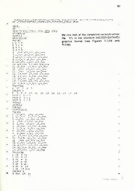
81
'?''SEn?E"TAn,YTE?1P:-?^.'^(^T<RT'^n,IPT-5 <° rri
EXIT.TC
3"T0TM-'JA'lErLl
Bonn1 1 ^ 51
2 1 1 (»
5 -^ -" 1
0'^:1 CT1) TTYr [ T< )
We now lock at the completed reconstruction
file. It's in the standard (MOTION-DATARD)
graphics format (see Figures 4-14d and
4-14e).
9 -1 ? .7""^
1" -1
1 1-"- :"'
1 r''.I
1 -' ! ^
1 " I
1 5 1
7-«
1 7 1. \,
I T :" rsq-i
? ni Y T vr.
1 'I'l i
:oLT'^'1 c
r 7 ^
3YT':; r
AYT5 '' ^
AVI? ^ 1
t-OTl.
J£*>^Er J^= lPrL3:^:'•C E N
^oriT-1
-1- .9''
-
T -21 -CITT
! 1 1 ?• 1 J 1 ^ I
.-70 11 .-(J I
5 1 . T'^ 1<7_<37I -T.-m=;
1
" .-ij-'1' ."^ 11 -'^ .T1'-''
7 11 ."^IQ ^.'^31 -9..no" 1 9 ,
7''': -.10;i -9,T'nt: 1 ;; .OQ^ - .C? 1 -O.TT^1'
1^.-?- -1-.T»(1 -Q.1^^
11 "- .0 7<; -1 1 .''P 1 -9 .Cllf^
12 111 -2-1, ""T ,Q,T,-ir,
13 -1 .IPQ -1 C ,Q 71 -0 .I'll
1 4 -1 T ,/!..-. .| ,, _->T/. .Q ^i-n1=; -1 .^jc -^.071 -<::.Tic
1'^ -? '.""'I .IT^ -Q..?1£1
PT.YJ TM31 t5 <? t6J t < ^ t7
J T7 ° 5
i t7 tn
5 TC 9 Tq
^ TC Q 1 T
7 TO 1^ TincniTiB 6
? Tld 1-1 11

82
'
—
"9'tro ir l2'
r' 10 ti(^ 12 Til11 Til 12 1312 Til 13 T12
r- 13 T12 13 1414 T12 14 15C0LTA9 7
c 15 T12 15 1 f>
1 6 Tl2 1 S 1
C0UTA3 5
c 1 7 T12 1 2
13 tl2 2 3
19 tl2 J T13
r 2£l Tl3 3 4
21 tl3 4 Tl422 tM 4 5
r 23 tM 5 6COLTAB 9
24 tl4 S rl5f^ 25 T15 S 7
26 T15 7 1n S27 T15 7 'M 7
c 28 Tl 7 7 529 Tl 7 5 'fl83-3 T13 8 1r5
EN1 82 S OSK PATES l-TT! !
FUCH3 \~ 329 PAGES OVEP ALLOCATI O-J! !
0:L2VA1E:L3P0PrL2BODYrSCElEPOI'JTS
1 -12.QK3 S.t^fis -3.3Ci!1
2 -l'^.ei'1 M.r'ci -3,r'?!13 -2.9 73 1 7.-'2 7 -J ."A'"
4 .5in? 2(1. '^'ici -3 .ri^n
5 7.^23 12 .977 -3.?i!"S IP.i'^n ii.c:'ci -s.'i'n7 1 7.^13 2 .SJS -3 ..1^1
8 19.719 -.194 -3.?''T9 12 .983 -S.Q'7 -3 .i""!
11 2 .9 73 -1 7.->2 7 -3 ..'ii:'
12 .ivii -2i.!"?T -3,;^:ici
13 -7.723 -12 .977 -3 .IT"14 -IT.r"-"" -l^.cm -3.'"l15 -17.T13 -2 .31 7 -3.7T11 S -r-i.Ti^ .111 -3.:i:';i
polygtn;C0LTA3 7
1 Tl 1^1C0LT49 !<;
2 Tl ! 2
3 Tl 2 t2
4 t2 2 3
5 t2 3 t3
S t3 3 4
7 t3 4 t4? TJ 4 s
9 t4 S ts1 '' t5 5 S
I 1 t5 « f i5
COLTAS <=
12 tS iS 7
13 f^ 7 t7

83
I 5 t7 H TB
1 6 tg 8 9
1 7 t"? 9 t9
I H T9 9 1 n
C0LTA9 6
19 t9 10 •H7I2^ Tl<' 10 11
21 Tl!^ 11 Tl 1
22 Til 11 12
23 Til 12 Tl224 TI2 12 1325 Tl2 13 T1326 TI3 13 1427 T13 M Tl4C0LTA3 9
28 TI4 14 1529 TM 15 T153n Tl 5 15 1 S
COLTA? 7
31 T15 1 fi Tl (?
32 tl 5 1 S Tl
C0LT!*3 6
33 M 13 12 11 nC0LTA3 9
34 M 'li 9 ? 7 S
35 2 1 IS 15 14EN0:L5END: DATA?
DAYUE0VP5DAY. 1AY 21. 1975 ^5:2.1: 1
1 -rOT

REFERENCES
[1] G. J. Agin, "Representation and description of curved objects," Stanford Artificial
Intelligence Lab., Memo AIM-173, Oct. 1972.
[2] G. J. Agin and T. 0. Binford, "Computer description of curved objects," in Proc. ofthe Third litlcrnntinnal Joint Conference on /Irtificial Intelligence, Stanford, Calif.,
Aug. 1973, pp. 628-640.
[3] B. G. Baumgart, "Geometric modeling for computer vision," Stanford Artificial
Intelligence Lab., Memo AlM-249, Oct. 1974.
[4] B. G. Baumgart, "A polyhedral representation for computer vision," in Proc. of 1975
National Computer Con/., Anaheim, Caiif., May 1975, pp. 589-596.
[5] T. 0. Binford, "Visual perception by computer," Proc. of the IEEE Conf. onSystems and Control, Miami, Dec. 1971.
[6] R. P. Burton, "Real-time measurement of multiple three-dimensional positions," U. of
Utah Computer Science Dept., Tech. Report UTEC-CSc-73-122, June 1973.
[7] L. Evans, Ph.D. Research Proposal, U. of Utah Computer Science Dept., 1974.
[8] A. D. Gara, R. F. Majkowski and T. T. Stapletoh, "A holographic system for
automatic surface mapping," General Motors Research Labs., Research Publication
GMR-1342, Warren, Michigan, March 1973.
[9] Geodolite Laser Distance Measuring Instrument, Data Sheet, Spectra-Physics,
Mountain View, Calif., Feb. 1969.
[10] R. E. Herron, "Biostereometric measurement of body form," Yearbook of Physical/Inlhropology, vol. 16, pp. 80-121, 1972.
[11] B. Julesz, "Toward the automation of binocular depth perception," Proc. of IFIPSCongress, 1962, North Holland, Amsterdam, pp. 439-443, 1953.
[12] M. D. Levine, D. A. O'Handley and G. M. Yagi, "Computer determination of depthmaps," Computer Graphics and Imago Processing, vol. 2, no. 2, pp. 131-151,Oct. 1973.
[13] R. Navatja and T. 0. Binford, "Structured description of complex objects," in
Proc. of the Third Iniemaiional Joint Conf. on /Irtificial Inielligence, Stanford,
Calif., August 1973, pp. 541-647.
ri4] F. I. Parke, "Computer generated animation of faces," U. of Utah Computer ScienceDept., Tech. Report LrrEC-CSc-72-120, June 1972.
85
[15] "Picosecond timing sharpens laser rangefinder resolution," Electronic Design,
vol. 15, pp. 48-50, July 19, 1974
[16] Y. Shirai and M. Suwa, "Recognition of polyhedrons with a rangefinder," in Proc. ofthe Second Intfrnational Joint Conf. on Artificial Intelligence, London, September
1971, pp. 80-85.
[17] B. S. Spreight, C. A. Miles and K. Moledina, "Recording carcass shapes by a Moire
method," Medical and llioloffical Enffinccring, pp. 221-226, March 1974.
[18] I. E. Sutherland, R. F. Sproull and R. A. Schumacker, "A characterization of ten
hidden-surface algorithms," /\CM Comfialing Surveys, vol. 6, no. 1, pp. 1-55,
March 1974.
[19] H. Takasaki, "Moire topography," /Ip/j/icrf Optic», vol. 9, pp. 1467-1472, 1970.
[20] D. Vickers, "The sorcerer's apprentice," U. of Utah Computer Science Dept.,
Tech. Report UTEC-CSc-74-078, July 1974.