NBER WORKING PAPER SERIES

THE "AUSTERITY MYTH":GAIN WITHOUT PAIN?

Roberto Perotti

Working Paper 17571http://www.nber.org/papers/w17571

NATIONAL BUREAU OF ECONOMIC RESEARCH1050 Massachusetts Avenue

Cambridge, MA 02138November 2011

This paper was produced as part of the project Growth and Sustainability Policies for Europe (GRASP),a Collaborative Project funded by the European Commission's Seventh Research Framework Programme,contract number 244725. Financial support by the European Research Council (Grant No. 230088)is also gratefully acknowledged. The views expressed herein are those of the author and do not necessarilyreflect the views of the National Bureau of Economic Research.

NBER working papers are circulated for discussion and comment purposes. They have not been peer-reviewed or been subject to the review by the NBER Board of Directors that accompanies officialNBER publications.

© 2011 by Roberto Perotti. All rights reserved. Short sections of text, not to exceed two paragraphs,may be quoted without explicit permission provided that full credit, including © notice, is given tothe source.

The "Austerity Myth": Gain Without Pain?Roberto PerottiNBER Working Paper No. 17571November 2011JEL No. E62,E65,F32

ABSTRACT

As governments around the world contemplate slashing budget deficits, the “expansionary fiscal consolidationhypothesis” is back in vogue. I argue that, as a statement about the short run, it should be taken withcaution. I present four detailed case studies, two – Denmark and Ireland – undertaken under fixedexchange rates (the most relevant case for many Eurozone countries today) and two – Finland andSweden - after floating the currency.

All four episodes were associated with an expansion; but only in Denmark the driver of growth wasinternal demand. However, after three years a long slump set in as the economy lost competitiveness.In all the others for a long time the main driver of growth was exports. In Ireland this occurred becausethe sterling coincidentally appreciated. In Finland and Sweden the currency experienced an extremelylarge depreciation after floating.

In all consolidations interest rate fell fast, and wage moderation played a key role in generating a gaincompetitiveness and a decline in interest rates. These results cast doubt on at least some versions ofthe “expansionary fiscal consolidations” hypothesis.

Roberto PerottiIGIER Universita' BocconiVia Roentgen 120136 MilanoITALYand CEPRand also NBERroberto.perotti@unibocconi.it

An online appendix is available at:http://www.nber.org/data-appendix/w17571

2 

 

1. Introduction 

Budget deficits have come back with a vengeance.  In  the  last  three years,    they have  risen  in 

virtually all countries, due to the recession and, in some cases,  to bank support measures.  What to do 

next is a matter of bitter controversy. For some, governments should start reining in deficits now, even 

though most countries have not  fully  recovered yet;  if done properly – namely, by  reducing spending 

rather  than by  increasing  taxes – budget consolidations are not harmful, and might  indeed result  in a 

boost to GDP. This  is one  interpretation of Alesina and Perotti  (1995) and Alesina and Ardagna  (2009) 

(AAP  thereafter), who  study all  the episodes of  large deficit  reductions  in OECD countries, defined as 

country – years where the cyclically adjusted deficit  falls by more than, say, 1.5 percent of GDP. They 

compare  the averages of macroeconomic variables before, during and after  these episodes, and  find 

that consolidations based mainly on spending cuts are typically associated with above average increases 

in  output  and  private  consumption,  while  consolidations  based  mainly  on  revenue  increases  are 

associated with recessions.  

For  others,  this  evidence  on  expansionary  government  spending  cuts  is  flawed,  and  the 

aftermaths of a recession are the worst time to start a fiscal consolidation. This is the  message of IMF 

(2010)  (IMF  thereafter).  The  heart  of  the matter  is  the methodology  used  to    estimate  a  cyclically 

adjusted change in the deficit, i.e. that part of the change in the deficit that is due to the discretionary 

action of the policymaker, as opposed to the automatic effects of the cycle on government spending and 

revenues. IMF argues  that the cyclical adjustment by AAP (in turn a variant of the methodology adopted 

by the OECD  in the Economic Outlook and by the  IMF  in the World Economic Outlook) fails to remove 

important  cyclical  components,  and  that  this  failure  can  explain  a  spurious  finding  of  expansionary 

budget  consolidations.  IMF  instead  estimates      “action  –  based”  or  “narrative”  measures  of  fiscal 

consolidations,  in  the  spirit  of  Romer  and  Romer  (2010),  and  uses  them  to  estimate  a  Vector 

Autoregression and compute  impulse responses of GDP and  it components to a discretionary shock to 

the government surplus. They conclude that all fiscal consolidations are contractionary in the short run. 

Although  not  based  on  a  formal  statistical  analysis,  Krugman  (2010)  argues  that  many  cases  of 

“expansionary  fiscal  consolidation”      were  driven  by  a  net  export  boom,  hence  the  mechanism  ‐ 

whatever it is ‐ is not replicable in the world as a whole.   

In  this paper,  I  argue  that  the  IMF  criticism of  the AAP    approach  is  correct  in principle  and 

represents an important potential advance; however, the implementation of the approach has problems 

of its own,  both in the way it computes action – based measures of fiscal consolidations and in the way 

3 

 

it    estimates  impulse  responses  to  fiscal  consolidations. On  the  other  hand,  large  consolidations  are 

typically multi‐year  affairs,  and  the means‐comparison methodology  of AAP  is  ill  suited  to  deal with 

these  cases.  Both  approaches  are  also  subject  to  the    reverse  causality  problems  that  are  almost 

inevitable with yearly data, and both  lump together countries and episodes with possibly very different 

characteristics.1  

For all these reasons, I argue that  one can learn much from detailed case studies. I present four, 

covering the    largest, multi‐year   fiscal consolidations that are commonly regarded as   spending based. 

Two  of  these  episodes  ‐  Denmark  1982‐86  and  Ireland  1987‐90  ‐  were  exchange  rate  based 

consolidations, while  the other  two – Finland 1992‐98 and Sweden 1993‐98  ‐ were undertaken  in  the 

opposite circumstances, after abandoning a peg. For each episode,  I do    two  things. First,    I compute 

action‐based measures of budget  consolidations, often using  the original documents, and  taking  into 

consideration  also  fiscal  action outside  the official budgets,  something  that was often overlooked by 

IMF.  As I will show, this typically results in smaller discretionary consolidations than   estimated by the 

IMF or the OECD, and  in a much smaller share of spending cuts. The reason  is that often governments 

used supplementary budgets during the year to undo some of the spending cuts of the January budgets, 

and also because the IMF often only considers spending cuts or tax increases.    

Second,  I study  in detail  the  timeline of budget consolidations,  the behavior of  interest  rates, 

wages and the exchange rate, and of GDP and its components, in order to try and learn something about 

the possible channels at work. I use contemporary sources, like the OECD yearly Economic Surveys (“ES” 

from now on) of each country, and country specific studies.  

In doing this,  I    focus on two very specific and narrow questions. First,  is    there evidence  that 

large  budget  consolidations,  particularly  those  that  are  based  mainly  on  spending  cuts,  have 

expansionary effects    in the short run?      I will have nothing to say regarding the medium‐ to  long‐run 

effects  of  fiscal  consolidations.  As  a  consequence,    I  will  have  nothing  to  say  about  their  social 

desirability:  it might well  be  that  reducing  government  spending  is  socially  desirable  even  if  it  has 

contractionary  effects in the short run.  

Second, if the answer to the first question is in the affirmative,  how useful is the experience of 

the past as a guide to the present? For  instance,  if fiscal consolidations were expansionary  in the past   

because they caused a steep decline in interest rates or inflation, it is unlikely that the same mechanism 

can be relied on  in the present circumstances, with  low  inflation and  interest rates close to zero. Or,  if 

                                                            1 Favero and Giavazzi (2011) study various dimensions of country heterogeneity and how this affects  the 

IMF estimates of the effects of consolidations.  

4 

 

consolidations were  expansionary mainly    because  they were  associated with  large  increases  in  net 

exports,  this  mechanism  is  obviously  not  available  to  a  large  group  of  countries  highly  integrated 

between them.  

That  private  consumption  should  boom when  government  spending  falls would  come  as  no 

surprise  to  believers  in  a  standard  neoclassical model with  forward  looking  agents. Although  in  that 

model alternative time paths of government spending and distortionary taxation can create virtually any 

response  of  private  consumption,  from  negative  to  positive,  the  basic  idea  is  straightforward;  lower 

government  spending means  lower  taxes and higher households’ wealth, hence higher  consumption. 

This is sometimes dubbed the “confidence channel” of fiscal consolidations.2 Lower taxes also mean less 

distortions,  hence  they    can  lead  to  higher  output  and  investment.  More  generally,  a  large  fiscal 

consolidation may signal a change  in  regime  in a country  that  is  in  the midst of a  recession, and may 

boost  investment through this channel. 

In open economies alternative effects may be at play. A fiscal consolidation might reinforce and 

make credible a process of wage moderation, either implicitly or by trading explicitly less labor taxes for 

wage moderation; this  in turn feeds  into a real effective depreciation and boosts exports. Or,  it might 

reinforce the decline in interest rates, by reducing the risk premium or by making a peg more credible. 

These alternative channels were highlighted  for  instance  in Alesina and Perotti  (1995) and  (1997) and 

Alesina and Ardagna (1998).  

The main conclusions of the case studies I present here are: 

(i) Discretionary fiscal consolidations are often smaller than estimated in the past, and spending 

cuts  are  less  important  than  is  commonly  believed. Only  in  Ireland were  spending  cuts    larger  than 

revenue increases; in Finland, spending cuts were a  negligible component of the consolidation.  

(ii) All stabilizations were associated with expansions in GDP. Except in Denmark (one of the two 

exchange  rate  based  stabilizations),  the  expansion  of  GDP  was  initially    driven  by  exports.  Private 

consumption  typically  increased 6  to 8 quarters  after  the  start of  the  consolidation. And  as national 

source data (as opposed to OECD data that turned out to be incorrect) show, the expansion in what was 

probably the most famous consolidations of all ‐ Ireland – turned out to be much less remarkable than 

previously thought. 

(iii) In Denmark the stabilization relied most closely on the exchange rate as a nominal anchor, 

and  as  such  is  of  particular    interest  for  small  EMU members  today. Denmark  relied  on  an  internal 

devaluation via wage restraint and incomes policies as a substitute for a devaluation. It exhibited all the 

                                                            2 Or “confidence fairy”, in the less charitable interpretation of Krugman (2011). 

5 

 

typical  features of an exchange  rate based stabilization:  inflation and  interest  rates  fell  fast, domestic 

demand  initially  boomed;  but  as  competitiveness  slowly  worsened,  the  current  account  started 

worsening, and eventually growth ground to a halt and consumption declined for three years. The slump 

lasted for several years.   

(iv)  In the   second exchange rate based stabilization,  Ireland, the government depreciated the 

currency before starting the consolidation and fixing the exchange rate within the European Exchange 

Rate Mechanism (ERM). Again wage restraint and incomes policies played a major role, but a key feature 

was  the  concomitant  depreciation  of  the  sterling  and  the  expansion  in  the  UK,    that  boosted  Irish 

exports and contributed to reducing the nominal interest rate.  

(v) The  two  countries  that  instead  floated  the exchange  rate while consolidating, Finland and 

Sweden,  experienced  large  real  depreciations  and  an  export  boom.  Also,  in  both  countries  inflation 

targeting was adopted  at the same time as the consolidations were started.  

(vi)  The  budget  consolidations were  accompanied  by  large  decline  in  nominal  interest  rates, 

from very high levels. 

(vii) Wage moderation was essential to maintain the benefits of  the depreciations and to make 

possible the decline of the long nominal rates. In turn, wage moderation probably had a powerful effect 

as a signal of regime change. 

(viii) Incomes policies were in turn instrumental in achieving wage moderation, and in signaling a 

regime shift  from  the past. Often  these policies  took  the  form of an explicit exchange between  lower 

taxes on  labor  and  lower  contractual wage  inflation. However,  the  international  experience  suggests 

that  incomes policies are effective  for a  few years at best. The experience of Denmark  in this study  is 

consistent with this.  

These  results are useful  to understand what are  the  typical mechanisms and  initial conditions 

that  are  associated with  expansionary  fiscal  consolidations.  Some of  the  conditions  that made  these 

consolidations expansionary (a decline in interest rates from very high levels, wage moderation relative 

to other  countries, perhaps  supported by  incomes policies)  seem not  to be applicable  in  the present 

circumstances of low interest rates and low wage inflation. The experience of the exchange rate based 

stabilizations, Ireland and Denmark, is particularly interesting, as it is conceivably more relevant for the  

Eurozone countries that are experiencing budget problems. Both countries managed to depreciate  the 

exchange rate prior to pegging and to the consolidation, an option that  is not available to members of 

the  EMU  except  vis  à  vis  the  non‐Euro  countries  as  a  whole.  Ireland  also  benefitted  from  the 

6 

 

appreciation of the currency of its main trading partner, the UK. In contrast, the Danish expansion was 

short lived, as it quickly ran into a loss of competitiveness that hampered growth for several years.  

The  timing  and  role  of  exports  growth  also    casts doubt  on  the  “confidence  explanation”  of 

expansionary  fiscal consolidations; an expansion that  is based on a real depreciation and a net export 

boom is also obviously not available to the world as a whole. 

However, even  in the short run budget consolidations were probably a necessary condition for 

output  expansion  for  at  least  three  reasons:  first,  they  were  instrumental  in  reducing  the  nominal 

interest rate;  second, they made wage moderation possible by signaling a regime change that reduced 

inflation expectations; third, for the same reason they were  instrumental  in preserving the benefits of 

nominal depreciation and thus in generating an  export boom.  

In my analysis, I do not use formal tools; I do not estimate consumption or investment functions, 

to test for instance whether there  are positive residuals during fiscal consolidations. Many consumption 

and investment functions  have been estimated for these countries before with a specific focus on these 

consolidation episodes,3 and I do not have anything to add to the existing estimates.  

I do not  consider political  factors,  such as whether    fiscal  consolidations are more  frequently 

observed  under majority  or minority  governments,  or  under  coalition  or  single  party  governments. 

Similarly,  I  do  not  address  the  role  of  budget  institutions,  such  as    whether  some  institutions  or 

processes are more conducive to effective consolidations, or the role of expenditure ceilings. These are 

all important issues, that have been dealt with elsewhere (see e.g. Alesina, Perotti and Tavares 1998 and 

Lessen 2000 on the  former issue,  and Guichard et al. 2007, Hauptmeier, Heipertz and Schuknecht 2007, 

Ljungman 2008, Hardy, Kamener and Karotie 2011, and Borg 2010 on the latter).  

I will also have little to say about the composition of spending cuts and revenue increases; again, 

this  is an extremely  important question, and  the original  focus of Alesina and Perotti  (1995), but one 

that is difficult to address in the context of the narrative approach that I use here.  

This paper has obviously numerous antecedents. The closest antecedent is Alesina and Ardagna 

(1998), who also look at case studies and emphasize the role of wage dynamics and incomes policies.  I 

defer a discussion of this and other papers to section 5.  

The outline of the paper is as follows. Section 2 presents a simple statistical model that allows  a 

unified treatment of the methodologies of the IMF and of AAP, and discusses the biases associated with 

                                                            3 See e.g. Giavazzi and Pagano (1990) for Ireland and Denmark, Giavazzi and Pagano (1996) for Sweden, 

Bradley and Whelan (1997) for Ireland, Honkapohja and Koskela (1999) for Finland, Bergman and Hutchsion (2010) 

for Denmark. 

7 

 

each. Section 3 focuses on the  IMF approach, and section 4 on the AAP approach. Section 5 discusses 

the relation with the literature. Section  6 presents the case studies. Section 7 concludes. 

    

2. A simple static model  

The  intuition for the AAP approach and for the   IMF criticism of that approach can be gathered from a 

simple static  model. The equation for the budget surplus is  

 

                              Δs = αyΔy + αp Δp + βyΔy + εs   αy > 0;   αp > 0;  βy > 0                                            (1)    

 

where s is the budget surplus as a share of GDP, y is the log of real GDP, and p is the log of asset prices. 

Due  to  the operation of automatic stabilizers,  the surplus  increases automatically  (i.e.  for given policy 

parameters  like tax rates and eligibility rules for unemployment benefits) when GDP  increases (αy > 0). 

The  surplus  also  increases  automatically when  asset  prices  increase,  because  of  their  effects  on  tax 

revenues  (αp  >  0).4  In  addition,  when  GDP  increases  policymaker  might  implement  systematic, 

countercyclical  changes to policy parameters (e. g., increase tax rates) to cool down the economy, and 

vice  versa  in  recessions:  this  is  captured    by    βy  >  0.  Finally,  the  random  component    εs  captures 

discretionary  actions  by  the  policymaker,  which  are  not  motivated    by  the  response  to  cyclical 

developments: for instance, actions motivated by ideology or long run growth considerations.  

I  allow GDP  to depend on    the pure  discretionary  component  εs   but  also on  the  systematic 

discretionary component   βyΔy, possibly with different coefficients: 

 

                                    Δy = γ1εs + γ2 βyΔy  + εy                                                         (2) 

 

In a keynesian world presumably γ1 < 0 and γ2 < 0. 5  

Finally, I assume that Δp is white noise: Δp = εp, and it is positively correlated with Δy: cov(Δy, εp) 

> 0.   εs  instead is a pure policy shock, uncorrelated with εp  or εy.  

                                                            4 See e.g. Morris and  Schuknecht (2007) and Benetrix and Lane (2011) 5 I am simplifying considerably here. While a textbook keynesian model like the IS‐LM model usually does 

imply γ1 < 0, virtually any contemporaneous or dynamic relation between the surplus and GDP can occur in a 

neoclassical model, with or without price rigidity. Only for simplicity I will sometimes refer to the case of  γ1 > 0 as 

“neoclassical effects” of fiscal policy, or “expansionary effects of fiscal consolidations”.    

8 

 

The  issue  of  estimating  the  fiscal  policy multiplier  can  be  interpreted  as  finding  a  consistent 

estimate of γ1 in equation (2) (of course in general this will be done in a dynamic context, such a Vector 

Autoregression,  but  this  simple  static model  is  enough  for  the  key  intuition).  The  econometrician, 

however,  in general does not observe  εs, but only  Δs. There are basically  two ways  to proceed next, 

which correspond to the two approaches by AAP and IMF.  

AAP apply a standard cyclical adjustment method, such as that by the OECD (see e.g. Fedalino, 

Ivanova, and Horton 2009): they use existing estimates of the automatic output elasticity αy to subtract  

αyΔy  from  the  observed  change  in  the  surplus.6  Hence  one  ends  up with  the  AAP measure  of  the 

cyclically adjusted surplus: 

 

ΔsAAP =  βyΔy + αpεp + εs                                                                                         (3) 

 

There are clearly two potential problems with using  this measure of the surplus, as emphasized 

by  IMF. The  first arises because    ΔsAAP  includes a  countercyclical  response by policymakers  to output 

shocks,  βyΔy,    which  is  positively  correlated  with  output  changes  since  βy    >  0.    I  call  this  the 

“countercyclical response” problem.7 The second problem arises because  ΔsAAP   contains a component, 

αpεp,      that  is positively correlated with output  since  standard cyclical adjustments do not correct  for 

asset price changes and αp > 0. I call this the “imperfect cyclical adjustment” problem.8  

                                                            6 The OECD constructs the cyclically adjusted change in the surplus using external estimates of the 

elasticity to output of each type of tax revenues. The actual  implementation of this approach by AAP is different: 

they first regress budget variables on the unemployment  rate, and then take the residuals of these regressions.  7 [The cyclical adjustment method] “omits years during which actions aimed at fiscal consolidation were 

followed by an adverse shock and an offsetting discretionary stimulus. For example, imagine that two countries 

adopt identical consolidation  policies, but then one is hit by an adverse shock and so adopts discretionary 

stimulus, while the other is hit with a favorable shock. […] The standard approach would therefore tend to miss 

cases of consolidation followed by adverse  shocks, because there may be little or no rise in  the [cyclically adjusted 

primary balance] despite the consolidation measures.” (IMF, p. 4). 8 “The first problem is that cyclical adjustment methods suffer from measurement errors that are likely to 

be correlated with economic developments. For example, standard cyclical‐adjustment methods fail to remove 

swings in government tax revenue associated with asset price or commodity price movements from the fiscal data,    

resulting in changes in the  [cyclically adjusted primary balance]  that are not necessarily linked to actual policy 

changes. Thus, including episodes associated with asset price booms––which tend to coincide with economic 

expansions––and excluding episodes associated  with asset price busts from the sample introduces an 

expansionary bias.” (IMF,  p. 4) 

9 

 

The action‐based, or narrative  measure of fiscal policy stance constructed by IMF   is an attempt 

to solve both problems by constructing a series for εs  directly, using the original official estimates of the 

effects on spending and revenues of each specific measure in a budget or in a spending or tax bill. Hence 

 

ΔsIMF = εs                                                                                                                                       (4) 

 

Now consider using these two measures of the discretionary fiscal stance   to estimate γ1.   The 

reduced form for output is 

 

Δy = kγ1εs + kεy ;               k = 1/(1 ‐ γ2 βy)                                                         (5) 

 

An OLS regression of Δy  on ΔsIMF  therefore gives:  

 

γIMF = kγ1 = γ1/(1 ‐ γ2 βy)                                                                                               (6) 

 

Hence, if the world is keynesian (γ1 < 0)  the IMF estimate of γ1   is biased towards 0 because of 

the  countercyclical  response problem.  Following  a unitary  realization of  εs, GDP  falls by  γ1;  then  the 

policymaker reacts, on average, by  increasing the surplus by   βy, which  leads to a decline    in output by 

|γ2βy|, and so on. If one  is  interested  in studying how much GDP reacts to a unit exogenous change  in 

the surplus, and not  in  these  indirect effects via  the policymaker  response,    the estimated coefficient 

from  the  IMF  approach  is biased  towards 0: one  estimates  a  less powerful  keynesian effect of  fiscal 

policy  than  in  the  true model. However,  it  is  likely  that  the  this particular bias of  the  IMF approach  is 

relatively small. 

Note  that  the problem  stems  from  the use of  annual data. With quarterly data,  it would be 

plausible to assume βy = 0, since the policymaker would not be able to learn about an output shock and 

react to it within three months. This was indeed the key identifying assumption in Blanchard and Perotti 

(2002). Note the parallel with changes in the Federal Fund rate target. Virtually all policy changes to the 

FFR are driven by countercyclical considerations. But, by assuming that changes in the FFR did not affect 

GDP within a month, with monthly data one can identify the component of the FFR forecast error that is 

orthogonal to GDP forecast errors. 

Now consider the AAP approach. The  estimated OLS effect of a regression of Δy  on ΔsAAP   is 

 

10 

 

                                            γAAP = cov(ΔsAAP, Δy)/var(ΔsAAP)  >  γ1                                                        (7)               

 

It  is   easy  to  show  that  the bias generated by  the AAP approach  is bigger  than  the  IMF bias, 

essentially because the AAP approach is affected both by the imperfect adjustment problem and by the 

countercyclical  response problem.9   An  incomplete  cyclical adjustment biases  the  coefficient  towards 

zero because  it generates a positive correlation between the change  in the AAP surplus and the error 

term  in  the  estimated  GDP  equation;  hence,  it  biases  the  results  again  towards  a  less  powerful 

keynesian effect of fiscal policy.  

Thus, methodologically  the  IMF  approach  is potentially  an  important  step  forward. However, 

contrary  to what  it  is  claimed,  it   does not explain  the  key  finding of AAP, namely  the expansionary 

effects of spending based consolidations. In addition, its implementation suffers from other problems of 

its own that complicate its interpretation. I now turn to these issues.   

 

3. The IMF approach 

In the simplest version of the IMF approach, one computes impulse responses from single 

equations regressions like  

 

               Δyt  =  ρ1 Δyt‐1 + … + ρk Δyt‐k + λ0 εs,t +  λ1 εs,t‐1 + …. +  λh εs,t‐h + ηt                                                      (8) 

 

In the more general case, one computes a VAR, in which lags 0 to h of εs,t appear as exogenous variables 

in each equation.  

Panel data VARs are always dangerous objects: they impose the same dynamics on potentially 

very different groups of countries (see Favero and Giavazzi  2011 on this), and  they introduce a bias 

from the presence of  lagged endogenous variables. Besides these well known problems, I will focus 

here on three others that are more specific to the particular application.  

 

 

                                                            9Note in particular that the  IMF approach is unbiased if βy  = 0, while the AAP approach continues to be 

biased. 

11 

 

A. Why  the IMF approach does not explain the expansionary fiscal stabilization results 

The  key methodological  point  of  IMF  is  that    the  bias  generated  by  the    imperfect  cyclical 

adjustment problem and by  the countercyclical  response problem can explain  the expansionary  fiscal 

consolidation results of AAP. This is incorrect.   

To understand why, note  that  IMF  and AAP  agree  that, on  average,  fiscal  consolidations  are 

associated with  a  recession  in  the  short  run. Where  they  differ  is  in  the  effects  of  spending    based 

consolidations: still contractionary according to IMF, expansionary according to AAP. 

However, contrary to  the claim by  IMF, the  imperfect cyclical adjustment bias cannot explain 

this difference    ‐    in  fact,  it goes  in  the opposite direction:  in other words,  removing  this bias would  

reinforce  the main  finding  of  AAP,  i.e.  that  revenue  based  consolidations    are  contractionary while 

spending  based ones are expansionary. In fact, if the IMF is correct, in periods of high growth, cyclically 

adjusted revenues are overestimated, hence the AAP approach    imparts a spurious positive bias to the 

correlation between increases in the surplus that are due to increases in revenues and GDP growth;  but 

the  AAP method finds a negative correlation. 

The  countercyclical  response  bias  also  is  unlikely  to  explain  the  expansionary  consolidations 

result.  For  discretionary  fiscal  policy  to  react  to  GDP  developments  within  the  current  fiscal  year, 

discretionary  fiscal  action  has  to  be  quick.  Changing  taxes  is  typically  easier,  and works  faster,  than 

changing spending; thus, as a first response policymakers will usually cut taxes  in response to negative 

shocks, and will increase taxes  in response to positive shocks. Again, this would impart a positive bias to 

the correlation between revenue based increases in the surplus and GDP growth, while the  AAP method 

finds a negative correlation. 

 

B. The censoring bias of the IMF approach 

IMF records only positive values of  εs, and sets all negative  values to 0. It is easy to show that 

censoring of the independent variable generates a bias away from 0 of the coefficient of interest:  Figure 

1, adapted from Rigobon and Stoker (2005), provides the  intuition. Rigobon and Stoker also show that 

the bias  can be substantial if a large share of the observations are censored; in the IMF study, these are 

about 60 percent of  the whole  sample. Hence,  if  fiscal policy has Keynesian effects,  censoring of  the 

independent  variable will  show  even  stronger  Keynesian    effects;  symmetrically,  if  fiscal  policy  has 

neoclassical effects, censoring will show even stronger neoclassical  effects. 

 

12 

 

C.   The standard error of the impulse responses 

IMF reports impulse responses with one standard error bands. While this is somewhat typical of the 

fiscal policy  literature,  I now agree with Ramey  (2011) that there  is no reason why only this particular 

literature  should deviate  from  the norm  in macroeconomics.10   The problem  is almost certainly more 

serious  in a panel VAR, because of the correlation of errors across countries, which  is bound to be an 

issue in this context; in the micro literature, this correlation  has been shown to lead to a downward bias 

in  the  estimated  standard  errors  by  a  factor  that  can  easily  reach  10  or more  (see  e.g. Angrist  and 

Pischke (2008) or Bertrand, Duflo and Mullainathan (2004). Failure to correct for this can therefore lead 

to  a  vast  underestimation  of  the  uncertainty  surrounding  the  estimated  impulse  response.  If  one 

considers  that  the  reported  impulse  responses would already not be  significant  if  two  standard error 

bands were used,  it  is doubtful how much  confidence we  should put  in  these estimates – a point  to 

which I will return below.  

 

D.   Omitting the countercyclical response in the IMF approach 

In computing its action – based measure of consolidations, IMF includes only those actions that 

can be ascribed to the goal of enhancing long run growth or reducing the deficit, thus excluding actions 

undertaken  with  the  goal    of  stabilizing    short  run  fluctuations. While  omitting  the  countercyclical 

response of  fiscal policy has an obvious motivation    for  the purposes of estimating    the multiplier of 

fiscal policy actions (as in Romer and Romer 2010), it can provide the wrong picture of the actual fiscal 

policy stance when trying to gather the size of a fiscal consolidation. It is also not easy to implement on a 

large set of countries, often without the help of primary sources like the original budget documents.  

Perhaps most  importantly,  it  is very difficult to  identify motives behind a certain policy action, 

and it must have been  even more difficult to contemporaries. It is conceivable that most policy actions 

are justified at some point by the desire to achieve such worthy goals as “growth” or “fiscal discipline”; 

finding the “true” motivation is likely to be nearly impossible. It is unlikely, however, that the public at 

the time would weigh differently the different measures, depending on their alleged motivation.  

For all  these  reasons, omitting  these actions gives a   distorted picture of  the  fiscal stance:  for 

instance, as I show later,  IMF concludes  that there was a large budget consolidation in Finland between 

1992 and 1995; but in fact there was hardly any, because spending cuts in the main budgets were often 

interspersed with spending increases in supplementary budgets that are largely ignored by IMF. Some of 

                                                            10 With apologies, having used one standard error bands in my own work.  

13 

 

these supplementary measures might have had a countercyclical motivation (if so, it  was rarely stated 

explicitly); more  likely,  these measures were  taken  in  response  to a political opposition  to  the earlier 

budget cuts ‐ perhaps within the government itself.  

In other cases,  the difference  in motivations was extremely – perhaps  too – subtle even with 

hindsight. For instance, in September 1982 the new Danish government introduced a package of budget 

austerity  in order  to curb  the  current account deficit.  In 1986  it  increased  taxes  to achieve  the  same 

goal. True,  the  former occurred  in a context of a much  larger budget deficit, but  the main motivation 

appears to have been the same.  IMF counts the former, but not the latter.  

 

4. Comparing averages in the AAP approach  

The AAP  approach  consists  of  comparing    average  values  of  several macro  variables  before, 

during and after large fiscal consolidations. First, AAP define a country‐year as a fiscal consolidation if in 

that year the cyclically adjusted primary balance improves  by, say,  at least 1.5 per cent of GDP.  Then 

they  compute  average  values  across  episodes  of  the  change  in  the  primary  surplus,  of  GDP,  of 

consumption growth, and   a number of other variables.,   “during” the year of the consolidation and  in 

the  two  years  “before”  and  “after”  the  consolidation.  They  repeat  the  exercise  separately  for 

“expansionary”  consolidations    (those  that  were  accompanied  by  an  increase  in  growth)  and  for 

“contractionary” ones.   

Finding the effects of fiscal consolidations  is not different from estimating  (possibly nonlinear) 

fiscal policy multipliers, an  issue that has been the object of a heated methodological debate recently. 

What  is  the  justification  then  for comparing averages of  large consolidations? Three possible  reasons 

come  to mind:  (i)  there  are  large measurement  errors,  which  are minimized  by  focusing  on  large 

consolidations;    (ii) the effects of fiscal policy can be nonlinear, so that  it makes sense to  isolate  large 

consolidations;    (iii)  consolidations are  random events,  that are  independent of  initial  conditions and 

other variables.  

However, even if assumptions (i) to (iii) above are correct, it is not clear what are the advantages 

of comparing means relative to running a VAR (the method adopted by the IMF, although subject to the  

censoring bias  illustrated above). But there are two more potential problems with the  implementation 

of the mean – comparison method. Both have to do with the fact that large consolidations are seldom 

14 

 

one‐year events.  I  illustrate them using the most recent  incarnation of the AAP approach, Alesina and 

Ardagna (2010). 

 

A.    Identifying multi‐year fiscal consolidations 

If, say, year t and t+2 are both consolidations years according to the definition above, year t+2 

appears both in the “after” average of the year t consolidation and in the “during” average of the year 

t+2  consolidation.  The  issue  becomes  trickier  because,  if  there  are  three  consecutive  years  of 

consolidation, t, t+1 and t+2, Alesina and Ardagna (2010)  consider  only year t as “during” and years t+1 

and t+2 as “after”; in other words, now year t+2 is no longer considered the “during” year of a different 

consolidation.  

 

B.   Comparing averages in multi‐year fiscal consolidations 

For all these reasons, it is difficult to  interpret a comparison of these averages.  An example of 

the possible complications that may arise is in Table 1. 11 The table  displays a comparison of the rate of 

growth of business investment “during” (year t) relative to “before” (years t‐1 and t‐2) the consolidation, 

and  “after”  (years  t+1  and  t+2)  relative  to  “during”, with  the  standard  errors  of  these  differences.12 

Clearly,  business investment booms “during” the expansionary consolidations, while it does not  budge 

during  the contractionary ones. But  then “after”  the expansionary consolidations business  investment 

declines for two years at almost the same yearly rate at which it increased “during” the consolidation, so 

that  by  year  t+2  it  is  below  the  level  of  year  t,  the  consolidation  year.  In  contrast,  after  the 

contractionary consolidations business investment increases for two years, and at the end of year t+2 it 

is well above its level in year t.  

The  case of business  investment  is extreme, as  the other macro variables do not exhibit  this 

pattern; also,  business investment  does not exhibit this pattern in Alesina and Perotti (1995) or Alesina 

and  Ardagna  (1998).  But  it  is  still  useful  in  order  to  illustrate  the  issue.  Exactly  because  fiscal 

consolidations  are  typically not one‐year  events,  it  is difficult  to  imagine  that  their    effects manifest 

                                                            11 The table does not exactly replicate  the results of Alesina and Ardagna (2010) because I have kept only 

those episodes for which there are complete data for the “after” period. In Alesina and Ardagna (2010), some 

episodes do not have an “after” average, hence the samples of “during” and “after” do not have the same size. To 

compute the standard error of the difference between the two samples, for each episode at time t I take the 

average of the years t+1 and t+2, I subtract the value at t, and I compute the average and standard error of all 20 

episodes thus constructed.    12 The standard error of the differences was not calculated in Alesina and Perotti (1995) or Alesina and 

Ardagna  (2010). 

15 

 

themselves  fully  in  the  year  of  the  consolidation  itself.    Hence,  it  is  important  to  understand what 

happens also after  the  consolidation, but  then  the potential  confusion between  “after” and  “during” 

becomes relevant.  

 

C.   Endogeneity and pre‐existing trends 

Conceptually, the means‐ comparison method is not different from a difference – in – difference 

estimator, in which one compares, say,  the difference in the rates of growth of GDP after and  before an 

expansionary consolidation with the same difference in contractionary  consolidations. In DD estimation, 

a key problem is that of pre‐existing trends: perhaps the finding that the rate of growth increases more 

in expansionary consolidations  is just a result of a pre‐existing stronger trend  in the   countries that we 

then assign to the “expansionary” group.   

This  problem  is  related  to  that  of  endogeneity  of  fiscal  policy.  We  have  seen  that  the 

imperfections  in the cyclical adjustment of revenues, of the type emphasized by  IMF,   cannot   explain 

the expansionary fiscal adjustment result of AAP. But there are other possible problems with the cyclical 

adjustment that may pollute the  interpretation of the evidence. There  is anecdotal   evidence that the 

cyclical adjustment may be particularly   problematic    in  large  recessions or expansions.  For  instance, 

during the recessions of the late eighties and early nineties, Finland and Sweden experienced  dramatic 

automatic increases in welfare related spending, of several percentage points of GDP in just one year. If 

this  is  true,    there  is  an  alternative  reading  of  the means  ‐  comparison  evidence  on  expansionary 

adjustments. Suppose there is an exogenous, persistent positive shock to growth: government spending 

as a share of GDP will fall GDP growth accelerates, giving the  impression of an expansionary, spending  

based consolidation while in reality fiscal policy was completely passive. This frequently heard criticism 

of the expansionary fiscal consolidation view is difficult to address, but at a minimum it seems to require 

a more satisfactory treatment of the dynamics of consolidations than just looking at the one year of the 

consolidation.  

 

5. Relation with the literature 

The  literature on  fiscal consolidations  is  large, and  it has been surveyed  in part  in Alesina and 

Ardagna (2010). Here, I will focus specifically on  recent work  that is more closely related to the present 

paper.  

16 

 

The closest antecedents of this paper  are Alesina and Ardagna (1998) and Broadbent and Daly 

(2010).  Alesina  and  Ardagna  (1998)  apply  the means‐  comparison method,  followed  by  ten      case 

studies. Most of the cases are one‐ or two‐year episodes;   only  Ireland and Denmark  last three years. 

The treatment of each case  is necessarily more concise than in the present paper. Like this paper, they 

emphasize the role of wage developments, although they do not study  in detail the evolution of wage 

negotiations  and  the  relation with  GDP  and  its  components.  Also,  their  conclusions  are  sometimes 

difficult to reconcile with  the evidence they present: as  Jordi Galí points out  in his discussion, relative 

unit  labor costs actually  increase  immediately after the start of the expansionary consolidations, while 

the  trade  balance  improves  significantly  during  the  recessionary  consolidations.  There  is  also  no 

discussion of the role of interest rates, that play instead a critical role in my analysis. 

Broadbent and Daly (2010)   also apply the means‐comparison method and present three short 

case studies, which display the salient features of each episode. The basic message is similar to Alesina 

and Ardagna (1998), with an additional emphasis on the role of the fall in interest rates. They point out 

correctly that interest rates declined in revenue based consolidations as well.  

Baker  (2010)  and  Jajadev  and  Konczal  (2010)  study  the  samples  of  fiscal  consolidations  of 

Alesina and Ardagna (2010) and Broadbent and Daly (2010) with a view to their applicability to current 

circumstances. They both point out that a key feature of the consolidations of the past is the scope for 

reducing interest rates, which is not available now. Jajadev and Konczal (2010) also argue that growth in 

the year preceding the adjustment was already strong on average in the sample of Alesina and Ardagna 

(2010)’s expansionary consolidations. 

Lilico, Holmes and Sameen (2009) also present six case studies, although they focus more on the 

budget and political processes of the consolidations.  

   

17 

 

 

6. Case studies 

 

I now present four cases studies. All four cover small, open European countries. The first two, Denmark 

1983‐86 and  Ireland 1987‐89, are  typically  regarded as  the  classical examples of  “expansionary  fiscal 

consolidations”. They are also  examples of exchange rate based stabilizations, in which a country pegs 

the exchange rate to obtain a rapid decline in inflation (although, as we will see,  things are not so clear‐

cut  in  the case of  Ireland). The next  two cases are Finland 1992‐98 and Sweden 1993‐98. These were 

also  associated  with  an  economic  expansion,  but  undertaken  under  opposite  circumstances  in  one 

important respect, i.e. after abandoning a peg and letting the currency float. 

  For each country,  I display  four tables, displaying my reconstruction of a narrative measure of 

yearly  discretionary  changes  in  spending  and  revenues,  various  types  of  interest  rates  and  spreads, 

various measures of exchange rates, unit labor costs, and inflation, and GDP and its components.  

 

 

 

DENMARK 

 

In 1980 and 1981 Denmark entered a recession. The deficit worsened quickly, from 1.5 percent 

of GDP  in  1979  to  11  percent  in  1982;  interest  payments  rose,  but  the  government  also  increased 

spending under pressure from rising unemployment; as a consequence, the primary  deficit increased by 

7.5 percent of GDP. The  recession was  relatively mild,  in part because  the  government devalued   or 

realigned  the Krone  several times during 1979‐82.13 In fact, in those three years the nominal effective 

exchange  rate  depreciated  by  about  15  percent  and  exports  increased  by  about  25  percent 

cumulatively.  

In  1982  GDP  expanded  strongly,  at  4  percent,  spurred  mostly  by  investment:  private 

consumption  was  subdued,  and  so  were  exports. Wage  dynamics  accelerated,  the  current  account 

deficit  rose  to  4 percent  of GDP,  and  the  Krone  came under  strong pressure;  to pre‐empt  a  further 

                                                            13 The Krone was devalued unilaterally  in November 1979, adjusted downward on the occasion of general 

ERM realignments in September 1979 and February 1982, while it stood firm when other currencies realigned in 

October 1981 and June 1982.   

18 

 

worsening  of  the macroeconomic  picture,  the  new  government  that  took  office  in  September  1982 

embarked in a medium run stabilization program. 

The  program  adopted  a  two‐pronged  approach  to  achieve  its  goals  of  enhancing 

competitiveness and reducing the budget deficit: it  explicitly ruled out devaluations, relying instead on 

the exchange rate as a nominal anchor; and emphasized incomes policies to achieve wage restraint. As 

we will see, the Danish episode exhibits all the hallmarks of a typical exchange rate based stabilization 

(see e.g. Ades, Kiguel and Liviatan 1993 and Detragiache and Hamann 1999): an  initial rapid decline  in 

inflation and nominal interest rates, a boom in domestic demand led by private consumption (especially  

durables) and, to a lesser extent, by private investment; a gradual  appreciation of the real exchange and 

a deterioration of the current account,  which eventually led to the undoing of the programme.   

 

Budget  timetable. Overall,  I  calculate  that  between  1983  and  1987    discretionary measures 

improved the primary balance by 8.9 percent of GDP, 55   percent of which tax  increases (see Table 2). 

IMF estimates instead a smaller consolidation, 6.7 percent of GDP, 35 percent of which tax increases.14 

IMF and  I agree almost exactly on the size and timing of spending cuts; but  IMF records much smaller 

tax  increases because  it omits the austerity measures of December 1985 and March 1986 (see below), 

totaling about 2 percent of GDP, on the ground that they were undertaken for countercyclical reasons. 

However, this underscores the difficulties of attributing a sharp motive to fiscal policy actions: officially, 

these measures were  undertaken  for  the  same  reasons  as  the  initial  1982  consolidation,  namely  to 

tackle the current account deficit.  

The  fiscal  consolidation  itself was  in  two  parts.  The  package  introduced  in  September  1982 

abolished  the automatic  indexation of  tax schedules,  froze unemployment benefits,  imposed a  tax on 

pension  schemes  (to be  replaced  from 1984 by a  tax on  their  interests and dividends earnings), and 

increased employers’ social security  contributions. The result was almost 2 percent of GDP in spending 

cuts and 1 percent of GDP in revenue increases in 1983.15 

After  the  draft  1984  Budget  was  rejected  in  December  1983,  elections  were  held  and  the  

government was confirmed in office. The April 1984 budget and various measures taken during the year 

cut spending by 1.2 percent of GDP and increased taxes by 1.5 percent of GDP. 

                                                            14 These numbers and the IMF numbers that  follow are based on Devries et al. (2011). 15 Local taxes also increased markedly (see 1982/83 ES, p. 26). 1983/84 ES, p. 9 also reports considerable 

reductions in local governments’ public investment (recall that “ES” stands for “OECD Economic Survey”). These 

effects have not been quantified.  

19 

 

In December of 1985, following continuing worsening of the trade balance in the second half of 

the year,    the government decided on a new austerity package, which was  followed by  two more  in 

March  and  October  1986.  All  three  relied mostly  on  tax  increases.  The  third  one  in  particular  (the  

”potato diet”) was worth 1.5 percent of GDP and  introduced a 20 percent tax on  interests (exceptions 

included  mortgages, loans to business and to students) and further restrictions on consumer credit. 

 

Inflation,  wage  dynamics,  competitiveness,  and  interest  rates.    Between  1980  and  1982 

relative unit labor costs in manufacturing fell by more than 15 percent, thanks to the depreciation of the 

Krone  and  a  good  productivity  performance.    Thus, Denmark  entered  the  consolidation  phase  after 

accumulating a  large depreciation. However,  the price of  this policy of devaluations and  realignments 

was high interest rates and a large differential vis à vis Germany: in September 1982, long‐term interest 

rates reached a peak of 23 percent.   

As we have seen, an important component of the September 1982 stabilization package was the 

use of the exchange rate as a nominal anchor. This policy gained credibility    in   March 1983 when the 

Krone  followed the DM  in appreciating  in an ERM realignment;  the  interest differential with Germany 

came down quickly.  A second precondition for the credibility of the policy was wage  restraint. This the 

government planned to achieve through active intervention in the wage negotiation process. 

The  incomes policies adopted were  in several steps. As part of  the comprehensive package of  

September 1982, the new government suspended all indexation of wages, salaries and transfer incomes 

until 1985; it limited the increases in public sector wages to 4 percent, with the explicit intent of making 

this a guideline  for  the wage negotiation between  the  trade unions and  the employers’ organization, 

coming up in March 1983.16 The subsequent wage agreement indeed followed closely these guidelines, 

implying a strong deceleration of the wage dynamics. The package also  froze the maximum amount of 

unemployment and sickness benefits until April 1986. After the election of spring 1984, the government 

approved   new  incomes policy measures, mainly an   extension of the suspension of wage and transfer 

indexation until March 1987.   

By  April  1983  long  term  interest  rates   were  down  to  14  percent.  Contemporary  sources17 

attributed  the  decline  to  the  strict  budget  policies,  to  the  increased  credibility  of  the  hard  currency 

policy when the Krone followed the DM  in the revaluation of March 1983, and to the moderate wage 

                                                            16 The government announced a tax cut of Krone 2.5bn (about  .5 percent of GDP) to support wage and 

salary freeze, but the tax cut  was later rejected by Parliament.  17 See e.g. 1982/83 ES p. 35, 1983/84 ES p. 12 and 1985/86 ES p. 17. 

20 

 

settlements. The  large capital outflows of  late 1982 also turned  into  inflows.  Interest rates kept falling 

following  the April 1984 budget which    included  further  incomes policy measures  (1983/84 ES p. 14). 

The liberalization of capital movements also contributed to reducing interest rates. 

After  the  failure  of  decentralized wage  negotiations  in  early  1985,  and  a  pessimistic    Public 

Finance  Report,  in March  1985    the  government  tried  to  have  tripartite  negotiations  but  was  not 

successful.  However,  it  decided  further  incomes  policy measures,  including  a  ceiling  on  public  and 

private sector salary  increases at   2 percent  in 1986/86 and 1.5 percent  in 1986/87.  It supported  this 

proposal by   a cut  in   employers’ social security contributions, financed by higher taxes on profits.18 By 

the beginning of 1986 long interest rates were down to 10 percent, and the differential with Germany to 

3 percentage points. 

Thus,  the  years  1983‐1985  were  years  of  wage  moderation,  helped  by  government  

intervention. 1986 displayed the first signs of wage pressure. The government was no  longer willing to 

provide wage targets for the 1987 wage negotiations; these  resulted in wage growth of 9 and 7 percent 

in 1987 and 1988. Two explanations have been offered  (see Andersen and Risager 1990 p. 173):  first, 

public  sector  workers  discontent;  second,  the  upcoming  1987  elections.  Also,  in  1986  the  nominal 

effective exchange rate started appreciating; as a result  of these developments, relative unit labor costs 

increased, by about 10 percent in 1986 and 1987.  

Thus, the benefits of incomes policies, to the extent that they were behind the wage restraint of 

1983‐85, were short‐lived: wage negotiations  in 1987‐89  largely undid the benefits of the earlier wage 

restraint.19 As  I  show below,    growth halted  from 1987  to 1989,  and  thereafter  remained  slow until 

1994.  

 

GDP and its components. Contrary to the case of the other countries that we will study,  growth 

was already high, at 4 percent, when  the September 1982   package   started  the consolidation, and  it 

stayed  there    until  1986.  The  recovery  was  broadly  based.  Investment  was  the  most  dynamic 

component, increasing at more than 10 percent per annum from 1982 to 1986, after falling by almost 30 

percent in 1980 and 1981. Consumption grew roughly at the same rate as GDP until 1985, and then at a 

remarkable 7.5 percent  in 1986. During this period average export growth was  less than 4 percent, far 

below that of the other countries of this study.  

                                                            18 In 1985 a radical reform of the budget process also took place. 19 As argued by Andersen and Risager 1990 p. 171, this is a common pattern with incomes policies. 

21 

 

 The  increase  in  consumption  in  1983  came  as  a  surprise  to  contemporaries,  against  the 

expectations  that  the March wage agreement would produce a decline  in  consumption; but because 

inflation also declined fast, real salaries remained constant. Initially the  consumption acceleration was 

due largely to durables: car registration increased by 36 percent; this  contributed  to about half of the 

increase in private consumption (see 1983/84 ES p. 20).  

Obviously also  the decline  in nominal  interest rates generated a wealth effect  that stimulated 

consumption. House prices increased by 60 percent in nominal terms (35 percent in real terms) between 

1982 and 1986. 1986/87 ES p. 32 calculates that this implied an increase by Kr. 200bn at current prices, 

or Kr. 100bn at 1982 prices, or about half of total private consumption in 1982. Before the 1986 “potato 

diet”, tax treatment of consumer credit was also extremely favorable: interest was totally deductible.20 

The stock market also boomed: real share prices almost doubled between 1982 and 1983.  

However, most  accounts  of  the  Danish  consolidation  stop  at  1986. What  happened  next  is 

equally interesting. As we have seen,  after a few years the attempt at “internal devaluation” failed, as 

the  incomes policy managed  to contain wage growth only until 1986.  In  the meantime,  the exchange 

rate appreciation and the lackluster productivity performance meant that relative unit labor costs slowly 

worsened.   Eventually,  the  trade balance worsened  so much  that  the  government was  compelled  to 

increase sharply interest rates and introduce other measures to cool demand. Between 1987 and 1989  

GDP growth halted, thereafter  it was about 1 percent per year until 1993; consumption declined by a 

cumulative 4 percent  between 1987 and 1989.  

Thus, Denmark displayed the standard pattern of exchange rate stabilizations, with a sudden but 

short  lived  boom  driven  by  domestic  demand21  and  a  gradual  worsening  of  competitiveness  that 

eventually  led to a prolonged slump. Ades, Kiguel and Liviatan  (1993)   attribute the boom  in domestic 

demand   also  to overconfidence: GDP and    consumption  forecasts  consistently exceeded  realizations 

during  those  years,  boosting  consumption  and  especially  investment.  Inflation was  also  expected  to 

decline faster than it did in reality, thus leading to a fast decline in nominal interest rates and in nominal 

and real wages.  

 

 

 

                                                            20 See Table 14 in 1986/87 ES, p. 33. 21 Interestingly, not all contemporaries had  the same perception: some viewed the recovery of those 

years as driven mostly by investment and exports: “The current recovery is more ‘healthy’  [than that of 1976‐79] 

because it is based on exports and investment” (1985/86 ES p. 23).  

22 

 

 

  IRELAND 

 

The story of the two Irish stabilizations has been told many times.22 Between 1982 and 1984 the 

government  attempted  to  cut  the  deficit  by  raising  personal  income  and  consumption  taxes.  The 

primary budget deficit did fall by 3.7   percent of   GDP between 1982 and 1986; this however was  less 

than the discretionary  increase in taxes (as estimated by IMF), due  to a lackluster growth performance 

and significant  increases  in social transfers and public wages.23 As a consequence,    in 1986 public debt 

was  110  percent  of GDP,  30  percentage  points  of GDP  higher  than  in  1982;  the  overall  deficit  had 

declined by only 2.5 percent of GDP, the primary deficit by  little more than 3 percent of GDP.24 Thus, 

what  is  regarded  as  the  prototypical  revenue  based  consolidation  was  not  a  success  story.  By  all 

accounts, in 1987 the mood in the country was gloomy, with a palpable sense of an impending crisis. In 

this paper,  I  focus on the second consolidation, that   started  in 1987 and  is widely associated with an 

impressive economic turnaround.  

 

Budget  timeline.  In  March  1987  a  new  minority  government  was  formed  by  the  former 

opposition party Fianna Fail. While Fianna Fail  had campaigned on a  populist platform, once in office it 

changed its mind and started a drastic fiscal consolidation, that lasted until 1989. In that year, the deficit 

was 2.6 percent of GDP, against 10.6  in 1986. In the same period, the primary balance switched  from a 

deficit of 2 percent of GDP    in 1986  to a  surplus   of 4.6 percent  in 1989. For  the  first  time  since  the 

beginning of the seventies public debt had stopped growing as a share of GDP, and actually declined by 

10 percentage points. GDP growth went from .4 percent in 1986  to 5.6 percent in 1989 and 7.7 percent 

in 1990.  

Estimating a narrative  measure of fiscal policy changes is particularly challenging in Ireland. The 

Irish  budget  process  at  the  time  was  extremely    complicated.  Some  decisions  for  year  t  –  except, 

                                                            22 See e.g. Dornbusch (1989) for the first stabilization, and Giavazzi and Pagano (1990), McAlesee (1990), 

and Honohan and Walsh (2002) for the second. 23 In 1985 and 1986 in particular, public sector wage increases, in part awarded by an arbitrator, caused a 

sizable overshoot of public spending. For instance, in 1985 the arbitrator awarded  a 10 percent increase to all 

school teachers in excess of the increase for all public sector workers. 24 Here and in the remainder of the paper the cyclically unadjusted budget figures refer to the general 

government and are usually taken from the OECD Economic Outlook.  

23 

 

crucially, most decisions on social transfers and government wages and employment  ‐   were   taken  in 

the Fall of year t‐1  in a document called the “Estimates”, while decisions on transfers and on taxes were 

taken in the January Budget of year t. To complicate things further, it is never exactly clear what  is the 

reference value  for a change  in, say, government spending  in these documents: whether the previous 

year  outcome,  or  some  notion  of  “constant  legislation”  spending,  or  the  Estimates  of  the  previous 

period, etc. 

Because of this complexity, it appears that IMF sometimes misses one of the two documents. A 

case in point is 1989: IMF – which, to repeat, only considers discretionary improvements in the primary 

balance  –  reports  a  value of  zero, because  the  1989   Budget  “introduced  a  number of  tax  cuts  and 

spending  increases” (IMF, footnote 54 p. 46). However, the 1989 Estimates also  introduced substantial 

spending cuts, almost double the spending increases of the Budget: as a result, 1989 was the third  year 

of the fiscal consolidation. 

More  importantly,  IMF    does  not  count  the  contribution  of  a  tax  amnesty  that  netted  2.1 

percent of GDP  in 1988, nor  the  introduction of  self assessment  that netted  .3 percent of GDP on a 

permanent basis. With  these  two measures,  the consolidation of  the years 1987‐88 would be equally 

divided  between  spending  cuts  and  tax  increases.  This  interpretation  is  consistent with  at  least  one 

account by an insider: “Briefly, there was no significant reduction in the real volume of current spending 

as a result of Bord Snip I [the expenditure review set up by the new government in 1987]. There was a 

further squeeze on capital spending, a mistake  in retrospect, but most of the adjustment came on the 

revenue side. The  ‘slash and burn’ stories about 1987,  references  to  the  finance minister as  ‘Mac  the 

Knife’, decimation of public  services  and  so  forth  are  just  journalistic  invention.  It never happened.” 

(McCarthy 2010, p. 45). 

Overall,  if one compares the    last year of the consolidation, 1989,   and the year preceding the 

consolidation, 1986, I estimate a discretionary change in  the primary balance of  3.6 percent of  GDP, all 

from spending cuts: almost half of these cuts fell on  capital spending.25 If one, like IMF, stops at 1988, 

then  I estimate an  improvement of 5.8 percent of GDP, almost equally divided between spending cuts 

and revenue  increases. As mentioned, this is due to the large amnesty of 1988. As a comparison,  over  

                                                            25 Ireland is the only country where I was able to estimate the breakdown between capital and current 

spending cuts. 

24 

 

the period 1987‐88 IMF calculates cumulative spending cuts by 3.1 percent of GDP and tax increases by 

.5 percent of GDP (IMF does not count 1989 as a consolidation year).26  

These  figures,   however,  ignore    temporary measures,  like  the  tax amnesty. When  temporary 

measures are  important, a more appropriate measure of  fiscal consolidation  is one  that   answers  the 

question: on average, how much were discretionary expenditures (taxes) lower (higher) in each year of 

the consolidation,  relative  to  the year preceding  the  start of  the consolidation?   This  is equivalent  to 

including all discretionary measures, weighted by the time they were  in effect. The figures  in this case 

are about 2.7 percent of GDP of spending cuts and .85 percent of tax increases.  

Thus,  the consolidation was significant, although perhaps   not so  large as  it  is often believed; 

and the contribution of tax increases was larger than usually assumed.   

 

 

Inflation, wage dynamics, competitiveness, and interest rates. In 1979 – three years before the 

first fiscal consolidation ‐ Ireland  had stopped pegging to the sterling and joined the European Exchange 

Rate Mechanism (ERM). Like in many exchange rate based stabilizations, this soon led to a large   decline 

in CPI inflation, which came down from a peak of 20.4 percent in 1981 to 3.8 percent in 1986 (see Table 

8).  

The  nominal  and  real  interest  rates  declined  until  1983,  as  the  punt managed  to  avoid  an 

appreciation  by  keeping  the  central  parity  during  two  realignments when  the DM  revalued,  and  by 

devaluing in 1983. But interest rate stopped falling afterwards, despite a further decline in  inflation, as 

the punt started appreciating. Thus, until 1986 real interest rates remained extremely high and the long 

term  interest rate differential with Germany  fluctuated between 6 and 5 percentage points. As Walsh 

(1993)  shows,  during  all  the  nineties  the  long  term  interest  rate  differential with  Germany  tracked 

closely  the sterling exchange rate: it increased when the sterling appreciated, and fell when the sterling 

depreciated.  

In  the year  to  the summer 1986,    the  Irish pound had appreciated by 20 percent vis‐à‐vis  the 

sterling pound. In  August 1986 the government devalued the Irish pound by 8 percent within the ERM. 

The 1986 devaluation, however, was the last one until January 1993: ERM participation was regarded as 

a nominal anchor policy (see Dornbusch 1989 and Giavazzi and Pagano 1990), and “the year 1986 was a 

                                                            26 The actual figures calculated by the IMF are 3.1 percentage points of GDP of spending cuts and .5 of tax 

increases. However, IMF uses  a figure for GDP at the denominator that turns out to be incorrect (see below); using 

the correct CSO figures gives the numbers I cite in the text. 

25 

 

watershed in Irish exchange rate policy” (Walsh 1993 p. 2).  Initially, long term interest rates kept rising, 

because  of  fears  of  budget  slippages  and  further  devaluations:  in  October  1986  they    reached  13 

percent.  Pressure  on  the  Irish  punt  and  on  long  term  interest  rates  abated  only when  the  sterling 

stopped depreciating  in early 1987.   Happily,  this  coincided with  the  second  fiscal  consolidation, and 

turned out to be a key difference relative to the first, failed  consolidation.  

The  years  of  the  failed  stabilization  1982‐86  saw  also  the  abandonment  of  centralized wage 

setting  and  the  move  to  decentralized  wage  setting  (see  Durkan  1992).  The  government,  having 

embarked in a process of tax increases, realized that it had nothing to offer at the negotiating tables and 

withdrew  from  the  process.  However,  this  did  not  prevent  a  strong  deceleration  of wage  inflation: 

average manufacturing earnings increased at a rate of 14.5 percent in 1982 and 7.5 percent in 1986, less 

than in the UK.  

As  part of the new stabilization package, in 1987 the government  returned to a tripartite wage 

bargaining process; in October it published the Program for National Recovery, which had been agreed 

with the  trade unions and the  employers. It included two wage agreements, one for the public sector 

and the other between trade unions and employers in the private sector. It set a maximum increase in 

wages by 2.5 percent  in 1988, 1989 and 1990. Table 8 shows  that wage  inflation came  further down, 

from 7.5 percent in 1986 to 5.4 percent in 1990;  real effective exchange rates based on unit labor costs 

and on wages in manufacturing, both of which had been worsening until 1986, improved dramatically. 27 

As Honohan and Walsh  (2002) put  it, “wage  restraint has been  the hallmark of  the  recovery”  (p. 28). 

“How much of this [improvement  in competitiveness] should be attributed to the new pay negotiation 

environment? Despite  the  inconclusive econometric results, most observers regard  the coincidence of 

timing  of  the  reversal  of  the  deteriorating  trend  in  competitiveness with  the  new  approach  to  pay 

bargaining  as  suggestive  that  the  latter  did  pay  dividends”  (p.  33).    Labor  relations  also  changed 

radically: the number of strikes fell dramatically relative to the previous period, and relative to the UK;28 

this  contributed  to  an  impression  of  regime  change  that  probably  had  important  effects  on  private 

investment.  

As Lane  (2000) writes,    low  inflation was a precondition  for wage  restraint:  the unions would 

probably not have accepted  the  latter without being  sure of  the  former.    In  this  respect,  the  second 

                                                            27  Measures of competitiveness based on unit labor costs in Ireland are somewhat misleading, because of 

the very large weight in manufacturing of a few multinationals  that, because of transfer pricing and highly valued 

patented products, exhibit enormous profits per employee and a very small share of labor costs: see Honohan and 

Walsh  (2002) p. 22.  28 See Hohanan and Walsh (2002) p. 32. 

26 

 

stabilization  benefitted  from  the  disinflation  process  of  the  first,  failed,  stabilization.  In  turn,  the  

spending cuts were also probably a precondition  for wage  restraint, as  they made possible a credible  

promise by the government to lower taxes in 1988 and 1989, by about  .6 percent of GDP, in exchange 

for wage moderation.29  

As wage moderation  set  in  the   market  learned  that  the  exchange  rate  policy was  credible; 

nominal interest rates  fell precipitously to 8 percent in 1988. The spread with the long German rate fell 

from 5 percentage points in 1986 to 2 in 1989, then it went further down. In this, Ireland was helped by 

the  appreciation  of  the  sterling,  which  instead  had  been  depreciating  during  much  of  the  first 

stabilization. Thus, because  the  largest decline  in  inflation had occurred before 1987,    the declines  in 

nominal interest rates afterwards were also largely declines in the real rate, contrary to the experience 

during the first stabilization, when real interest rates increased.30   

 

GDP  and  its    components.  GDP  growth  was  0  in  1986.  In  the  first  year  of  the  second 

stabilization, 1987,  it rose to   3.5; it then reached almost 8 percent in 1990. By all measures, the second 

stabilization was a spectacular success.  

For a  long time   growth was driven by exports, that rose at an average rate above 10 percent 

between 1987 and 1990. This strong performance of exports started  in the second half of 1986, hence 

before the fiscal consolidation, and can be  attributed to two  factors: the growth of export markets, on 

average  8.8  percent  between  1985  and  1988,  in  particular  in  the  UK;    and  the  improvement  in 

competitiveness  following  the August 1986 devaluation, coupled with  the wage  restraint of 1987 and 

1988. 

Domestic demand was  subdued  for  a  long  time.  The  average  growth  rate of  consumption  in 

1987‐88 was   2.8 percent,  the same as  in 1985‐86  ‐  two recession years. Data on sales are consistent 

with the notion that consumption growth was modest: sales started to pick up only in 1988:Q3, but until 

then they remained below the 1985 and 1986 levels. 31 

                                                            29 Both tax cuts are missed by  IMF; they do not show explicitly in Table 6, were the 1988 tax cut is 

summed algebraically with the effects of the tax amnesty.  30 The steep decline in nominal interest rates is likely to have prompted a large increase in the value of 

government debt held by  households;  the exact effect is difficult to quantify since we do not have measures of 

government debt at market values.  31  Contemporary sources had the same impression:  in October 1987, hence about three quarters after 

the budget plans had been announced, the 1987/88 ES writes: “Trade statistics for the first three quarters  of the 

year  show a major expansion  of exports due to renewed growth of the exports of foreign companies  and to the 

strong rise  in United Kingdom imports [….] At constant prices, the external balance improvement is the major 

27 

 

The pattern exhibited by gross  fixed capital  formation  is even starker:  it was negative  in 1987 

and 1988, and turned positive only    in 1989 after 7 consecutive years of negative numbers. Figures for 

the aggregate can be misleading, because of the large cuts to public sector investment, and the Central 

Statistical Office   data do not have a breakdown between government and private gross  fixed capital 

formation.  But investment in machinery and equipment tells a similar story: it increases by less than 2 

percent in 1986 and 1987, well below the rate of growth of GDP, and starts growing at  17 percent only 

in 1989. 

Why this difference with the standard story of the Irish miracle? The OECD data typically used in 

international comparisons are very different (see Table 10 ): for instance, relative to CSO data the rate of 

growth of GDP  in 1988  is more  than 2 percentage points higher  in OECD data,  the  rate of growth of 

consumption in 1989 is more than double, and gross fixed capital formation turns positive (and large, at 

5 percent) already in 1988. 

As it turns out, following an inquiry of mine the OECD Statistical Directorate realized that it had 

not  received  the  revised  Irish  national  accounts  for  1970‐1995,  hence  these   were  not  available  for 

incorporation in the Economic Outlook database. The OECD has communicated to me that the Irish CSO 

data are more appropriate for historical analysis. 32 

Thus,  there  was  no  explosion  of  domestic  demand  in  Ireland  following  the  second  Irish 

consolidation: for almost two years after the start of the consolidation, GDP growth was driven  largely  

by exports. At the same time,  the budget consolidation of 1987‐89 was substantial but not “brutal”, and 

tax increases (particularly from the tax amnesty) were significant.  

But what can account for the difference between the two consolidations, 1982‐86 and 1987‐89? 

After all, as Giavazzi and Pagano (1990) correctly point out,   exports were strong even during the first 

stabilization  (see  Table  9).    The  most  often  cited  difference  is  in  the  composition  of  the  budget 

consolidation, which was tax‐ based during the first and spending based during the second. It is easy to 

see why it could matter: spending cuts made room for tax cuts on labor income, which in turn enhanced 

competitiveness; wage reductions in the public sector, that were announced repeatedly during the first 

stabilization  but  implemented only during  the  second,  enhanced  the  confidence  in  the  ability of  the 

government  to  carry out  its programme  and  set  the  stage  for more wage moderation  in  the private 

sector (see Hoanhan 1989 p. 205) .  

                                                                                                                                                                                                factor behind the projected 2 percent  expansion in GNP this year.  By contrast, most of the component of 

domestic demand  remain rather depressed .. Retail sales have been weak for most of the year ..” (p. 30). 32 Historical data for Ireland have been temporarily suspended in the new issue of the Economic Outlook 

pending a complete integration of the new series. 

28 

 

Table 8 shows that a second  important difference was the behavior of wages and relative unit 

labor costs  in manufacturing. They were growing, although at declining rates,  in  the  first stabilization, 

and declining during  the  second. As we have  seen,  the  change  in  labor  relations was  the  key  to  this  

development. All indicators of competitiveness worsened dramatically in 1986, the year growth came to 

a halt after two years which averaged growth above 2.5 percent, only slightly below the figure for 1987‐

88. 

A third difference, that  is rarely mentioned,33  is the behavior of real  long term  interest rates.34 

Table 7 shows that these were high and rising during the first stabilization, and declined at the beginning 

of  the  second  stabilization.  The  decline  of  the  spread  with  the  German  long  rate  was  particularly 

pronounced. The  reason  is  that during  the  first  stabilization  inflation and  inflation expectations were  

coming down  fast because of  the depreciation of  the  sterling; but precisely  for  the  same    reason  the 

Irish rates remained high. As mentioned above,  in this sense the second stabilization could afford  low 

real rates because inflation had come down already and the sterling was now appreciating for the first 

two years.  Thus, although both stabilizations were exchange rate based, the second benefitted from the 

appreciation of the sterling, which improved competitiveness and allowed the nominal and real interest 

rate to decline.35   

It  is  also  important  to  understand  the  similarities  and  differences  between  the  second 

stabilization  and  the experience of Denmark.  Like  Ireland, Denmark pursued an exchange  rate based 

stabilization, and achieved a remarkable decline in nominal and real interest rates. In both countries the 

exchange based stabilization was  initially sustained   by   wage moderation and the  involvement of the 

government in the wage formation process. On the other hand,  Denmark’s consolidation occurred in a 

boom, rather than in a recession as in Ireland; and it was not spending based, but it was equally divided 

between revenue increases and spending cuts. 

But perhaps the key difference is that in Denmark the expansion that occurred at the time of the 

consolidation  was  driven  by  domestic  demand;  in  Ireland,  for  a  long  time  it  was  driven mostly  by 

exports.    Three  possible  explanations  stand  out.  During  the  consolidation  Denmark  suffered  from  a 

deterioration of  relative unit  labor costs, while  Ireland experienced an  improvement,   because of  the 

                                                            33 Dornbusch (1989) emphasizes the role of high real interest rates during the first stabilization, but was 

writing just at the beginning of the second stabilization.  34 Because I do not have data on expected inflation over this period, I compute the real long term interest 

rate as the difference between the nominal rate and inflation over the last year.  35 Also, during the first stabilization, the primary deficit came down as fast as during the second, but 

started from a higher level:  high real interest rates combined with still high primary deficits meant growing debt. 

29 

 

appreciation of the sterling, of a few realignments in which it did not follow the DM, and a much better 

productivity performance. Second, Denmark experienced a house price and a stock market boom at the 

time of the consolidation, both much stronger than  in Ireland, partly because of the steeper decline  in 

interest rates. Third, the term structure remained steeper in Denmark, providing an incentive for higher 

consumption.36    

It is useful to summarize the main conclusions. (i)  The Irish budget consolidation of 1987‐89 was 

smaller and more tax based than previously thought; (ii)   for several quarters the   GDP expansion was 

mostly  export‐driven;  consumption and private investment recovered 6 to 8 quarters after the start of 

the  consolidation,  and  their  recovery was   more  subdued  than  previously  thought;    (iii)  in  1987‐89 

Ireland  pursued  an  exchange  rate  based  stabilization,    after  a  substantial  devaluation    and  a  large 

decline in inflation; but, crucially, it did manage to depreciate  the punt during a few realignments, and 

relative  to  the  sterling;  (iv)  this  second  stabilization  saw  a  decline  of  long  rates  and  an  even more 

pronounced  decline  of  the  differential  with  Germany.  This  was  helped  by  the  appreciation  of  the 

sterling, which statistically  is associated with a reduction  in the Irish rates. The decline  in the  long rate 

was not large, but it was in marked difference to the first stabilization, which had suffered from high and 

increasing    real  rates;    (v)    the decline  in  inflation made possible a substantial wage moderation,  that 

was  also  instrumental  in  enhancing  competitiveness  and  in  signaling  a  change  in  regime;      incomes 

policies by the government were instrumental in consolidating the process of wage moderation;  (vi) the 

budget consolidation probably played an  important role  in   ensuring the credibility of a regime shift to  

low inflation, wage moderation, and lower  interest rates.  

 

   

                                                            36 Giavazzi and Pagano (1990) offer another explanation: the more advanced credit markets  for 

consumers in Denmark. However, as observed by Drazen (1990) in his comments to the paper, the numbers on the 

change in consumer credit in the two countries do not seem to be large enough to explain the difference in the 

behavior of consumption. Three more factors are often mentioned as explanations of the Irish boom of 1987‐90 

(see e.g. Whelan 2010): the inflow of EU structural funds, investment by multinationals,  and emigration, which 

eased unemployment. The first two, however, started in earnest after 1989 (see e.g. Barry 2000); the role of the 

latter is difficult  to assess, and deserves more scrutiny. Obviously, it  can still be the case that the large investment 

by multinationals in the nineties was made possible by the change in regime signalled by the budget cuts of 1987‐

89.   

30 

 

 

FINLAND 

 

The next two case studies, Finland and Sweden, differ from the first two  because they pursued 

a budget consolidation after abandoning a peg. During the eighties, in Finland financial deregulation and 

tax incentives for housing investment fuelled a boom characterized by huge capital inflows, large private 

sector indebtedness, and asset price inflation. In the early nineties Finland suffered the worst recession 

of  all OECD  countries.  Real GDP  fell  by  14  percentage  points  between  the  1990  peak  and  the  1993 

trough. The recession was exacerbated by four factors: a banking crisis when asset prices collapsed,  the 

demise of the Soviet Union, a deterioration of the terms of trade, and the decision to defend the peg to 

the ECU against speculative attacks. By late 1991 the central bank had raised the overnight lending rate 

to 50 percent, while the one month  interbank Helibor rate stood at 27 percent. Because  inflation was 

low,  real interest rates were extremely high throughout the recession. The government finally agreed to 

devalue in November 1991 by 12 percent vis à vis the Ecu; the decision to float the Markka in September  

1992 was followed by a further depreciation by 15 percent. 

Meanwhile, the budget balance moved from a surplus of 7 percent of GDP in 1989 to a deficit of 

8 percent in 1993. Contrary to other countries, interest payments did not play a role: the change in the 

primary  balance was  virtually  identical. During  the  same  years,  government  debt  as  a  share  of GDP 

quadrupled, from 14 percent to 56 percent. 

By the end of 1992 Finland was widely considered the basket case of Europe. Then, like in many 

other  countries,  GDP  growth  turned  positive  in  late  1993;  in  1994  it was  4  percent,  the  highest  in 

Europe, and it stayed there for several years. 

 

Budget timeline. IMF reports a discretionary improvement in the budgetary position in each of 

the  years  1992  to  1997, with  cumulative  spending  cuts  of  12.1  percent  of  GDP  and  a    cumulative 

consolidation of 11.4 percent of GDP. It is easy to see why this is probably  a considerable overestimate 

of  the  discretionary  consolidation.  Over  the  same  years,  the  cyclically  unadjusted  primary  balance 

improved by about 7 percent of GDP;  thus, cyclical conditions would have caused a worsening of  the 

balance by 4 percent of GDP – yet  except for 1992  these were years of very high growth. 

This can be seen even more clearly for the years 1994 and 1995, which saw a cumulative GDP 

growth of about 8 percent. The cyclically unadjusted primary balance improved by 3.4 percent of GDP; 

IMF reports a cumulative discretionary improvement by 5.1 percent of GDP, once again implying that in 

31 

 

those two years cyclical factors caused an increase in the deficit by almost 2 percent of GDP despite the 

exceptionally high growth. 

My  reconstruction of  the discretionary  improvement  in  the budget balance over  the 1992‐98 

period is less than half  the IMF estimate: 4.9 percent of GDP against 11.4 (see Table 11). Spending cuts 

amount  to only 1 percent of GDP;  the  remaining 4 percent are  tax  increases. Thus,  this was a much 

smaller fiscal consolidation than  in  IMF data, and  it was revenue based.  In contrast,  in the  IMF data  it 

was all spending based. 

What  explains  this  discrepancy  between  the  IMF  estimates  and  mine?  Often  several 

supplementary budgets undid the budget cuts decided in the January budgets; in some cases IMF misses 

these  supplementary budgets,  in others  it mentions  them but does not  consider  their effects on  the 

ground that they had a countercyclical motivation.37 As I discuss above, I am skeptical that motivations 

can be detected so sharply; and in many cases the spending increases were probably motivated not by 

countercyclical considerations, but by political pressure to ease the effects of the January budget cuts. In 

fact, many of these spending increases were financed by tax increases, which is also the reason why IMF  

reports virtually no tax  increases: for   example,  in 1996 supplementary budgets  increased revenues by 

1.75  percent  of  GDP,  but  this  does  not  appear  in  the    IMF  estimates.  In  the  end,  omitting  these 

discretionary changes offers a highly distorted picture of discretionary fiscal policy during these years. 

In addition, my data (and, a fortiori, the IMF data) almost certainly underestimate the extent of 

tax  increases  during  the  consolidation,  because  the  effects  of    changes  in  tax  rates  are  not  always 

quantified in the budget documents. Thus, between 1992 and 1994 several measures to increase taxes 

were adopted (see e.g. the  list  in   1993 ES pp. 81 and 84 and 1995 ES p. 104) but their effects did not 

appear in any document.  

Note  also  that  during  these  years  the  central  government  increased  spending  on  several 

measures  to  support  the banking  system, by about 10 percent of GDP between 1991 and 1995;  38  if 

these were  included,  cumulatively    spending would  increase,  instead of decreasing, over  these years. 

Banking  support  operations were      indeed widely  perceived  as  government  spending,   much  as  the 

support of the banking system in the US and the UK has been a major item of contention in the debate 

on fiscal policy during the recent financial crisis. As it is well known, however, exactly how to treat bank 

support measures is not obvious: for instance, a capital injection is a financial investment to be counted 

                                                            37 See IMF footnotes 30, 31 and 32, pp. 29‐31. 38 This figure includes loans, preferred capital, and ordinary shares acquired by the Government 

Guarantee Fund; I do not consider guarantees, which would add another 6.5 percent of GDP. See 1996 ES p. 48 for 

details on bank support measures by type and year. 

32 

 

below  the  line,  but  a  capital  injection  in  a  bank  that  is  essentially  bankrupt  is    a  capital,  or  even  a 

current,  transfer. Furthermore,  some  loans are  repaid, but  repayment might escape measurement as 

they are   seldom given the same prominence as the original loan.  

Turning to actual developments, the fiscal consolidation process of 1992‐98 can be divided into 

two phases, which coincide with two different governments. In 1992, the government elected in March 

1991 announced a  fiscal  consolidation program based on a new medium‐term  framework.  I estimate 

that by the end of  its mandate  in 1994 this resulted    in a cumulative  improvement  in the discretionary 

balance by 4.4 percent of GDP, equally divided between  spending cuts and  tax  increases. During  this 

period, the only year with a substantial spending cut was 1993; 39 this was followed  in 1994 by a  large 

tax increases of 2.3 percent of GDP, from two supplementary budgets.40 The discretionary improvement 

in  the primary balance estimated by  IMF over  the  same period  is double my estimate, all of  it  from 

spending cuts. 

Contemporaries  could  be  forgiven  if  they  did  not  realize  that  a  brutal  spending  based 

consolidation was under way. Headline numbers did not help:  the general  government deficit was still 

6.1 percent of GDP  in 1995, above  the 1992  level;  similarly, government debt as a  share of GDP was 

larger in 1995 than in 1992. 

In April 1995 a new government took office, and immediately introduced an austerity package. 

However,   my data and  IMF present  two  radically different pictures of what happened next. Overall, 

between 1995 and 1998 I estimate a further improvement in the discretionary primary balance of only 

.8 percent of GDP; during this period, discretionary   spending actually  increased by  .5 percent of GDP. 

IMF instead estimates spending cuts by 4.7 percent of GDP and tax cuts by 1.3 percent of GDP. 

The  difference  on  the  spending  side  is  due  to  two  years,  1995  and  1997.  In  1995  the  new 

government   did make good on the promise to cut   spending by 2 percent of GDP: this    is the number 

reported by  IMF. However,  the  January budget of  the outgoing government had already  included an 

increase  in government  spending by 2.4 percent of GDP, due  to  the costs of EU   accession  (spending 

increased  mainly  because  the  government  compensated  farmers  for  the  abolition  of  tariffs).  Two 

supplementary budgets, one in late 1994 and the second in early 1995, further increased 1995 spending 

                                                            39 Here and it what follows it is sometimes hard to attribute spending cuts to a given year. The third 

supplementary budget  increased spending by 1.7 percent of GDP; because it was approved in October  1992,  I 

attribute it to 1993. If instead it were to be attributed to 1992, it would imply a  spending cut in 1992 and an  

increase in spending in 1993.  40 There was a further increase in taxes because of the decision to postpone tax refunds to 1995; of 

course this also shows up in 1995 as a tax cut. 

33 

 

by almost 1 percent of GDP.41 As a result,  in 1995 discretionary spending actually  increased,  instead of 

falling as reported by IMF. 

In 1997 a  spending cut of 1 percent of GDP was offset by a   cut  in employers’ contributions, 

largely due to the  Incomes Policy Agreement of late 1995 (see below) that traded wage moderation for 

tax cuts. However, once   supplementary budgets are  included,   spending actually  increased, and other 

tax increases nearly offset the tax cuts. 

On  the  tax  side,  the  difference  between my  data  and  IMF  is mostly  due  to  1996,  when  a 

supplementary budget introduced a tax hike by 1.5 percent of GDP that was ignored by IMF. 

 

 

Inflation, wage dynamics, competitiveness, and interest rates.  Thanks to the November 1991 

devaluation  and  the  subsequent  floating    of  the Markka  in  November  1992,  the  nominal  effective 

exchange rate depreciated by 25 percent between 1991 and 1993 (see Table 13). 42  

At the beginning of the consolidation phase interest rates were very high, due to the attempted 

defense of the Markka. They  fell fast after the devaluation and subsequent floating: the three months 

Helibor (interbank) interest rate fell from 17 percent in September 1992 to 7.5 percent in June 1993. The 

spread with the German  interest rate had disappeared by   that date. The  long term  interest rates also 

came down considerably, but because the  short term interest rate had been pushed up by the defense 

of the Markka against very strong speculation, the yield curve from negatively sloped became positively 

sloped  at  the  beginning  of  1994, with  the  differential  between  the  10  year  and  the  three months 

interest  rate  at  about  2  percent  (this  is  about  the  time  when  durable  consumption  ‐  but  not  yet 

nondurable consumption ‐ started to grow: a steep yield curve with very low short interest rates is the 

right time to buy durable goods). 

What made possible this decline in nominal interest rates? Like in the  case of Ireland, there are 

three  plausible  candidates.  First,  the  budget  consolidation,  although  as we  have  seen  smaller  than 

commonly thought, signaled a change of direction. Second, an  often overlooked event that took place 

at the same time was the formal adoption  in February of 1993 of  inflation targeting, signaling another  

change  in  regime. Third,  the nominal depreciation  translated  into a  real depreciation  thanks  to wage 

                                                            41 Another supplementary budget in November 1995, which I attribute to 1996, further increased 

spending by . 6 percent of GDP in connection with the employment measures of the Employment Programme of 

fall 1995. 42 In October 1996, Finland joined the European Monetary System, thus ending the period of floating. 

34 

 

moderation.43  During 1992‐93 manufacturing unit labor costs fell by almost 15 percent, and relative unit 

labor costs fell by an impressive 45 percent.  Two successive centralized wage agreement44 in 1992 and 

1993  froze  contractual wage  increase.  This  contributed  to  the  enormous  gains  in  competitiveness  in 

those two years.  In fact,  in   June 1993 the 1993 ES wrote ”When market confidence  improved   by the 

announcement  of  a  government  package  aiming  at  fiscal  consolidation,  and  by  a  pay  settlement 

implying no wage  increase  for  a  second  consecutive  year,  short  term  interest  rates were  allowed  to  

ease gradually” (p. 33). 45 

In 1995, however,  these gains in competitiveness were threatened by a combination of nominal 

appreciation and wage slippages. At  the end of 1993,  the government had disengaged  itself  from  the 

tripartite  negotiations  for  1994,  and  negotiations  became  entirely  decentralized.    After  a moderate 

round of wage settlements for 1994, negotiations  in  late 1994 set contractual wage  increases for 1995 

at 4 percent, partly  as  a  consequence of  the  tightening  labor market. That  year     hourly earnings  in 

manufacturing  increased by 7 percent, unit  labor  costs by 5 percent,  and  relative unit  labor  costs  in 

manufacturing by 15 percent, thanks also to the appreciation of the nominal exchange rate. 

As inflation expectations rose and doubts about the stabilization emerged, interest rates moved 

back up    in 1994 and especially  in 1995. To counteract the  inflation threat posed by the   decentralized 

wage settlements of late 1994, between December 1994 and February 1995 the Central Bank increased 

its tender rate by 1 percentage point. 

At this point, the government, concerned that high wage settlements could undo the effects of 

its austerity package, returned to the table and promoted a new round of tripartite negotiations. These 

ended with an Incomes Policy Agreement in October 1995 that set an increase in wages of 1.8 percent in 

1996 and 1.3 percent  in 1997. The government contributed by enacting a tax cut  for 1997. Unit  labor 

costs  stopped growing  in 1996 and  then declined  in 1997;  relative unit  labor  costs declined by more 

than 5 percent  in each of  those  two years. At  the  same  time,  consumer  confidence picked up again. 

Between October  1995  and March  1996,  after  the October  1995  Incomes  Policy Agreement  and  the 

                                                            43 Honkapohja and Koskela  (1999) p. 36 put forth an interesting reason for wage moderation in Finland 

during these years: they argue that the costs of job loss are increasing in the level of household indebtedness. 44 In Finland wage negotiations occur first at a centralized level; although not binding, they set the tone 

for the more decentralized negotiations that follow. 45 Obviously interest rates came down in the rest of Europe too, but the descent was particularly fast in 

Finland. Because expected inflation also declined fast, thanks to the moderate wage agreements, real interest 

rates stayed fairly high. However, if government debt is net wealth and it is in nominal terms, a decline in the 

nominal interest rate pushes up its real value. 

35 

 

Employment Programme, the Central Bank cut the tender rate  by 3.5 percentage points (see 1996 ES p. 

38).  

Thus, the 1995  Incomes Policy Agreement explicitly traded wage moderation for  lower  income 

taxes  and  social    insurance  contributions;  this  agreement  was  instrumental  in  gaining  back 

competitiveness after the slippages of 1994 and 1995.  It  is here that the modest budget cuts of those 

years might  have  had  the most  important  effect:  by  enabling  the  government  to  enact  tax  cuts  in 

support of  the  incomes policies  that started  in  late 1995. As  Jonung, Kiander and Vartia  (2008) write: 

“perhaps the biggest change in the 1990’s in Finland  was the adoption and wide acceptance of a policy 

of long term wage moderation” (p. 35). 

Indices  of  consumer  confidence  shed  further  light  on  this,  by  allowing  tracking  changes  in 

consumer  sentiment  at  a  higher  frequency.  Three  questions were  asked  in  Finland  before  1995:  on 

unemployment  prospects  if  the  country,  on  the  intention  to make major  purchases,  and  on  general 

economic conditions  in  the next 12 months  (see Figure 2).46 Confidence had started  improving before 

the fiscal consolidation. It fell in the second half of 1994 when tripartite wage negotiations broke down, 

and recovered at the beginning of 1996, when the Incomes Policy Agreement was reached, but also one 

year after  the austerity programme by  the new government was announced. Thus,  the  timing of  the 

measure  of  consumer  confidence  also  points  to  the  importance  of  wage  agreements  and  incomes 

policies as a signal of regime change. 

 

 

GDP and its components. As the large depreciation set in,  exports began to pick up in 1992, and 

grew at an average rate above  10 percent per year until 2000 (see Table 14). However,  all components 

of private domestic demand  initially  tanked. GDP  growth was  very negative  in 1992,  still negative  in 

1993, and turned positive only  in 1993:3.   After that  it posted an average growth of about 4.5 percent 

until the end of the decade. 

Total  private  consumption  started  increasing  only  in  1994,  after  which  it  grew  at  above  3 

percent until the rest of the decade; and private investment only in 1995, after which it kept growing at 

a very fast pace, between 8 and 19 percent. 

Thus,  the  recovery was  initially driven by exports;  in  fact,  still  in  July 1996  the 1996 ES  could 

write: “The divergence between exports and domestic demand has become very pronounced  indeed, 

                                                            46 I multiply the balance of the responses to the unemployment question by ‐1, so that an increase in the 

index means higher confidence that unemployment will decline.  

36 

 

with the former  at 150 percent  and the latter at 75  percent of their 1990 levels by 1995” (p. 3). It was 

not until 1999 that domestic demand recovered the level of 1990. 

In  addition,  as we  have  seen,  1994 was  a  year  of  large  tax  increases;    1995 was  a  year  of 

spending  increases, preceded and  followed by even  larger  tax  increases. Thus,  it  is hard  to  relate  the 

consumption recovery to  the crowding in effects of a spending based consolidation that did not actually 

take place in those years. It is tempting instead to relate it to the export boom and lower interest rates.  

As consumption of durables turned around in late 1993, the Ministry of Finance’s 1994 Economic Survey 

wrote  that “although  […]  the  tightening of  taxation  [emphasis added] continued  to reduce disposable 

income,  [at  the  beginning  of  1994]  brighter  economic  prospects  and  a  fall  in  interest  rates  raised 

consumers’ propensity to consume” (p.48). 

Although  the Finnish  consolidation was  implemented under a  float and  the  Irish one under a 

peg, the two episodes have several features in common. On close inspection, they are both  smaller and 

more  revenue  based  than  previously  thought  –  in  fact,  in  the  case  of  Finland  spending  cuts  were 

minimal,    at  around  1  percent  of  GDP  cumulatively.  Both  entered  the  consolidation  phase with    a 

substantial depreciation ‐ which was truly large in the case of Finland. In both countries the  initial GDP 

expansion was  driven  by  exports,  and  started  before  the  consolidation;  the  growth  of  consumption 

started 6 to 8 quarters after the start of the consolidation; in both wage moderation played a key role; in 

both  incomes  policies  by  the  government  were  instrumental  in  consolidating  the  process  of  wage 

moderation after a temporary slippage that threatened to derail the stabilization. In Finland, it was only 

after the  new round of wage negotiations signaled a regime change that consumption and investment 

picked up. In addition, in Finland inflation targeting further contributed to a signal of regime change, and 

the nominal interest rate displayed a large decline.  

Why then did the appreciation and  loss of competitiveness of 1994‐95 not  lead to a prolonged 

slowdown like in Denmark almost ten years before? One can only speculate, but one plausible reason is 

that  the  government  intervened  to  restore wage moderation,  thus  enhancing  the  credibility  of  the 

stabilization  programme;  second,  because  of  booming  demand  abroad  exports  kept  growing  at  a 

remarkable rate even during the temporary slowdown, except for 1996. 

37 

 

SWEDEN  

The Swedish boom of the eighties and bust of the early nineties had several features in common 

with  Finland.    Financial  liberalization  with  tax  incentives  for  borrowing  fuelled  a  consumption  and 

housing boom, followed by a recession that started in 1990. Inflation fell, and the real interest rate rose 

drastically, causing a housing bust and a banking crisis. By 1993 unemployment was at 7.5 percent, and 

the budget deficit had  increased to 11.2 percent of GDP from a surplus of 3.2 percent    in 1989. Like  in 

Finland, this dramatic worsening of the budget balance was not due to  interest payments: the primary 

budget showed exactly the same deterioration. 

Throughout the recession the government, like in Finland, tried to defend the exchange rate to 

anchor inflation expectations, causing a steep loss of competitiveness and a drastic hike in interest rates. 

Eventually,  like  in Finland,  the Krona had  to abandon  the peg and began  floating  in November 1992.  

GDP kept declining  in 1993,  then  it  turned around  in 1994, when  it grew at 4 percent, a pace  that  it 

maintained to the end of the decade except for a brief respite in 1995 and 1996, when growth slowed to 

about 2 percent. By 1998 the budget was in surplus,  reaching  3 percent of GDP in 2000. 

 

Budget timeline. The consolidation started in 1993, and was over by 1998.47 During this period, I 

estimate a discretionary change in the primary balance by 8.4 percent of GDP, 40 percent of which from 

spending cuts. IMF estimates a total improvement in the primary balance by 10.5 percent of GDP,  more 

than 60 percent of which from spending cuts. Most of the   difference between my estimate and IMF’s 

estimates can be explained by the same  factors that were at play  in Finland:    IMF does not count the 

higher spending due to EU accession, and it does not count some spending increases in supplementary 

budgets. 

As a caveat,  it  should be noted that it is extremely difficult to reconstruct discretionary changes 

in  spending and  revenues  in Sweden. For 1993 and 1994,  IMF  is based on  two documents:  the  fiscal 

consolidation program of September 1992, and the 1993 Budget. For the crucial years 1995 to 1998, it is 

based  entirely  on  the  reconstruction  of  consolidation measures  by  the Ministry  of  Finance, with  its 

breakdown  by  calendar  year, made  ex  post  in  1998.  However,  this  source  is  not  entirely  reliable, 

because  it  is  partly  a  political  document;  in  fact,  it    includes  only measures  that  cut  spending  or 

increased  taxes,  and  reproduces  as  is  the  original  deficit  reduction  plan  of  September  1994,  later 

published as the Convergence Program for EU membership. 

                                                            47 On the Swedish consolidation, see Henriksson (2007). 

38 

 

As an example, that document includes as part of the consolidation Kr 20bn (1 percent of GDP)  

of extra revenues needed to finance the costs of EU accession, but  it does not record on the spending 

side the Kr 20bn of new spending due to EU accession. In addition, like in the case of Finland,  IMF does 

not consider  several  supplementary budgets and other measures not  in  the main budgets or  in  fiscal 

consolidation programs; and, for example,  it only counts spending cuts  in the 1995/96 budget, but not 

spending increases. 

Unfortunately, hard data on the  items not  included  in the Finance Ministry document of 1998 

are hard to get, partly because  ‐ again like in the case of Finland ‐  the effects of some  tax  or spending 

changes have not been quantified. 

And  again  like  in  Finland,  the  result  is  that  IMF  most  likely  overestimates  the  size  of  the 

consolidation, and the share of spending cuts in it. For instance, IMF shows a fiscal consolidation in 1993 

of 1.8 percent of GDP. However, the primary surplus declined by more than 3 percent of GDP; it seems 

unlikely  that  the  recession  by  itself would  have  been  responsible  for  a  deterioration  of  the  primary 

balance by about 5 percent of GDP  (the OECD cyclically adjusted primary surplus  falls by 1 percent of 

GDP). As  it  turns out,  if one  includes  the effects of  a  June 1993  supplementary budget  and of extra 

spending decided in the fiscal consolidation package of September 1992, there was hardly any decline in 

spending. 

Another example is 1998, when  IMF reports  a discretionary consolidation of 1 percent of GDP. 

This exceeds  the  increase in the unadjusted primary surplus, implying that, without discretionary action  

the primary balance would have worsened, despite growth at 4 percent, the highest in the decade. The 

explanation  is that  IMF does not  include extra spending for 1.1 percent of GDP,   due to the five point 

programme to enhance job creation, which does not appear in the official Finance Ministry rendition of 

fiscal consolidation. 

Turning to the main policy developments,  like  in Finland one can distinguish two phases  in the 

Swedish  consolidation.  The  first  one  runs  from  1993  to  1994,  and  corresponds  to  the  centre‐right 

coalition government. The  second phase  corresponds  to  the Social‐Democratic government  that  took 

office after the elections of  September 1994. 

During the first phase the discretionary  improvement  in the balance amounted to   3.4 percent 

of GDP, almost equally divided between spending cuts and tax increases. The second phase started with 

the November 1994 consolidation package, which  together with  the 1995/96 Budget of  January 1995 

and a supplementary budget in April envisaged a cumulative consolidation by about 4.5 percent of  GDP 

by 1998. With subsequent modifications, this became about 5 percent of GDP, about two thirds of which 

39 

 

were tax  increases.  In particular, note that  in 1995‐96 the primary budget  improved by 4.5 percent of 

GDP, but spending cuts amounted to only about .7 percent of GDP. 

 

Inflation, wage  dynamics,  competitiveness,  and  interest  rates.  Like  Finland  and,  to  a  lesser 

extent, Ireland, Sweden entered the budget consolidation phase with a large depreciation following the 

decision  to  float  the Krona  in November 1992  ‐ by almost 20 percent  in 1993  in nominal  terms on a 

multilateral basis. Like in Ireland and Finland, long interest rates came down quickly, from 10 percent to 

7 percent by the end of 1993; the differential with Germany also declined sharply to 1.5 percent.  

The  candidate  explanations  for  the  decline  in  interest  rates  are  the  same  as  in  Finland  and, 

except for the  inception of  inflation targeting, as  in  Ireland. First, budget austerity. Second,  in January 

1993  –  hence,  at  the  same  time  as  the  start  of  the  fiscal  consolidation  ‐  Sweden  adopted  inflation 

targeting.  Although    it  was  decided  that  it  would  become  fully  operational  in  1995,  the  Riksbank 

announced that  it would pursue a target of 2 percent as of 1993. Inflation remained subdued  in 1993, 

less than 4 percent, and there was no upward pressure on  inflation expectations after the float. Third, 

the  consolidation years were  characterized by a  surprising degree of wage moderation, with a  short‐

lived slippage in 1995 and 1996 – again like in Finland. Apart from the slack in the labor market and the 

sense of national crisis, one important reason for wage moderation was probably  the move to inflation 

targeting in January 1993, which  “had a profound impact on the behavior of labor market participants” 

(Jonung et al. 2008, p. 37). As a sign of confidence  in the Riksbank,   a non‐indexed two‐year collective 

agreement was signed in  1993 for 1994 and 1995, and three year agreements were signed thereafter. 

Sweden  did  not  have  a  formal  incomes  policy  agreement  like  Finland.  But  the  “internal 

devaluation”  package  of  September  1992  added  to  the  exchange  rate  depreciation,  by  reducing 

employers’ social security contributions, financed by an increase in VAT. Thus, in early 1991 a two‐year 

centralized  bargaining  kept  contractual wage  increases  at  a  low  2  percent  for  1993, which  including 

wage drift would have  caused hourly wages  to  increase  at  about 4 percent;    the  reduction  in  social 

security contributions decreased  it back  to 2 percent  (see 1993 ES p. 7). Also, unlike Finland,  in 1993 

Sweden had a tax reform that reduced the marginal tax rate on labor. 

Together with improvements in productivity and the depreciation of the nominal exchange rate, 

this implied large declines in multilateral unit labor costs, by almost 40 percent between 1992 and 1995! 

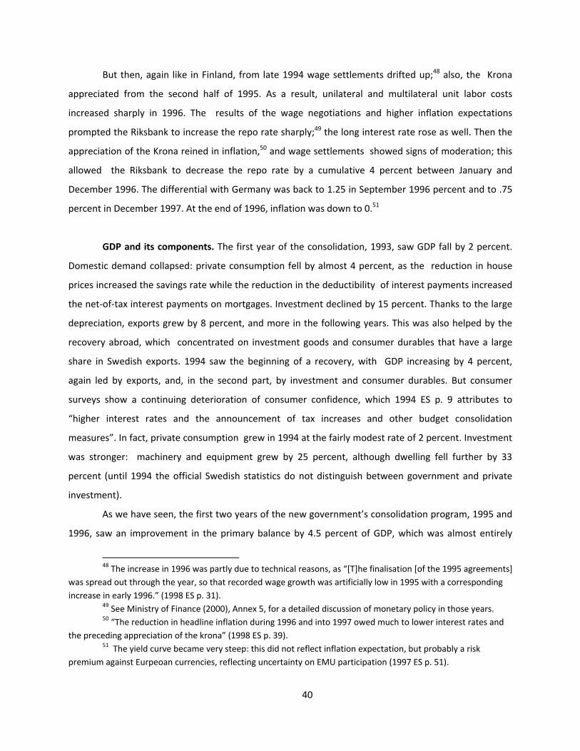
40 

 

But  then, again  like  in Finland,  from  late 1994 wage settlements drifted up;48 also,  the   Krona 

appreciated  from  the  second  half  of  1995.  As  a  result,  unilateral  and multilateral  unit  labor  costs 

increased  sharply  in  1996.  The    results  of  the  wage  negotiations  and  higher  inflation  expectations 

prompted the Riksbank to increase the repo rate sharply;49 the long interest rate rose as well. Then the 

appreciation of the Krona reined in inflation,50 and wage settlements  showed signs of moderation; this 

allowed    the  Riksbank  to  decrease  the  repo  rate  by  a  cumulative  4  percent  between  January  and 

December 1996. The differential with Germany was back to 1.25 in September 1996 percent and to .75 

percent in December 1997. At the end of 1996, inflation was down to 0.51 

 

GDP and  its components. The first year of the consolidation, 1993, saw GDP fall by 2 percent. 

Domestic demand collapsed: private consumption fell by almost 4 percent, as the   reduction  in house 

prices increased the savings rate while the reduction in the deductibility  of interest payments increased 

the net‐of‐tax interest payments on mortgages. Investment declined by 15 percent. Thanks to the large 

depreciation, exports grew by 8 percent, and more  in the following years. This was also helped by the 

recovery abroad, which   concentrated on  investment goods and consumer durables  that have a  large 

share  in  Swedish exports. 1994  saw  the beginning of a  recovery, with   GDP  increasing by 4 percent, 

again  led by  exports,  and,  in  the  second part, by  investment  and  consumer durables. But  consumer 

surveys  show  a  continuing  deterioration  of  consumer  confidence, which  1994  ES  p.  9  attributes  to 

“higher  interest  rates  and  the  announcement  of  tax  increases  and  other  budget  consolidation 

measures”. In fact, private consumption  grew in 1994 at the fairly modest rate of 2 percent. Investment 

was  stronger:   machinery  and  equipment  grew  by  25  percent,  although  dwelling  fell  further  by  33 

percent  (until 1994  the official Swedish  statistics do not distinguish between government and private 

investment). 

As we have seen, the first two years of the new government’s consolidation program, 1995 and 

1996,  saw an  improvement  in  the primary balance by 4.5 percent of GDP, which was almost entirely 

                                                            48 The increase in 1996 was partly due to technical reasons, as “[T]he finalisation [of the 1995 agreements] 

was spread out through the year, so that recorded wage growth was artificially low in 1995 with a corresponding 

increase in early 1996.” (1998 ES p. 31). 49 See Ministry of Finance (2000), Annex 5, for a detailed discussion of monetary policy in those years. 50 “The reduction in headline inflation during 1996 and into 1997 owed much to lower interest rates and 

the preceding appreciation of the krona” (1998 ES p. 39). 51  The yield curve became very steep: this did not reflect inflation expectation, but probably a risk 

premium against Eurpeoan currencies, reflecting uncertainty on EMU participation (1997 ES p. 51). 

 

41 

 

financed by taxes. GDP growth remained high in 1995 at around 4 percent. It was still driven by exports 

and by investment; private consumption remained subdued, at 1 percent. Most of the modest recovery 

in consumption was led by durables and car registration: “Other indicators, such as retail sales, convey 

an impression of continued retrenchment  in consumer spending”.( 1997 ES p. 19) 

Then in the second half of 1995 and first half of 1996  growth slowed markedly, in parallel with 

the hike  in  interest  rates,  the appreciation of  the Krona   and  the  relapse  in wage moderation. Export 

growth declined sharply, and in the first half of 1996  GDP growth fell to 0; only housing investment was 

strong. Private consumption and exports started recovering in the second half of 1996. By 1997 exports  

had recovered their high rate of growth of above 10 percent 

Thus, except  for 1996, during the consolidation period exports always exhibited a growth rate 

near or well above 10 percent. In contrast, private consumption grew slowly after the rapid declines of 

1990  to  1993,  and  it    really  started  picking  up  only  in  1998,  towards  the  end  of  the  five    year 

consolidation. Still in 1998 the perception was that growth was driven by exports and investment: “The 

economy  is  now  in  the  fifth  year  of  an  expansion  which  has  relied  on  exports  and  business  fixed 

investment for most of its momentum.”   (1998 ES p.  17) 

In  many  respects,  the  Swedish  consolidation  of  the  nineties  is  similar  to  the    Finnish 

consolidation that occurred at the same time, and to  the Irish consolidation of the previous decade. Like 

them,  its  discretionary  component  is  smaller  and  more  revenue  based  than  previously  thought. 

Particularly  like  in  Finland,    the  budget    consolidation  was  preceded  by  a  large    depreciation.  The 

expansion was  driven initially by export and by investment; the growth of consumption was muted for a 

long time after the start of the consolidation. Wage moderation was an important factor that reinforced 

the decline in interest rates;  in turn, tax reductions made possible by spending cuts were important in 

consolidating  the process of wage moderation after a  temporary slippage. Like  in Finland,  the budget 

consolidation was contemporaneous with the introduction of inflation targeting.  

  

7. Conclusions 

In this paper, I have  looked more closely at four episodes of  large fiscal consolidations. Two of 

these  episodes  occurred  immediately  after  pegging  the  exchange  rate,  while  two  occurred  in  the 

opposite circumstances,  immediately after  floating.    I have argued    that  typically  these consolidations 

relied on tax increases to a much larger extent than previously thought.  

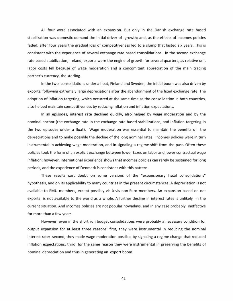
42 

 

All  four  were  associated  with  an  expansion.  But  only  in  the  Danish  exchange  rate  based 

stabilization was domestic demand the  initial driver of   growth; and, as the effects of  incomes policies 

faded, after  four years the gradual  loss of competitiveness  led to a slump that  lasted six years. This  is 

consistent with the experience of several exchange rate based consolidations.   In the second exchange 

rate based stabilization, Ireland, exports were the engine of growth for several quarters, as relative unit 

labor  costs  fell  because  of  wage  moderation  and  a  concomitant  appreciation  of  the  main  trading 

partner’s currency, the sterling.  

In the two  consolidations under a float, Finland and Sweden, the initial boom was also driven by 

exports, following extremely large depreciations after the abandonment of the fixed exchange rate. The 

adoption of inflation targeting, which occurred at the same time as the consolidation in both countries, 

also helped maintain competitiveness by reducing inflation and inflation expectations.     

In  all  episodes,  interest  rate  declined  quickly,  also  helped  by wage moderation  and  by  the 

nominal anchor (the exchange rate  in the exchange rate based stabilizations, and  inflation targeting  in 

the  two  episodes  under  a  float).   Wage moderation was  essential  to maintain  the  benefits  of    the 

depreciations and to make possible the decline of the long nominal rates.  Incomes policies were in turn 

instrumental  in achieving wage moderation, and  in signaling a regime shift from the past. Often these 

policies took the form of an explicit exchange between lower taxes on labor and lower contractual wage 

inflation; however, international experience shows that incomes policies can rarely be sustained for long 

periods, and the experience of Denmark is consistent with this pattern.  

These  results  cast  doubt  on  some  versions  of  the  “expansionary  fiscal  consolidations” 

hypothesis, and on its applicability to many countries in the present circumstances. A depreciation is not 

available  to EMU members, except possibly vis à vis non‐Euro members. An expansion based on net 

exports    is not available  to  the world as a whole. A  further decline  in  interest  rates  is unlikely    in  the 

current situation. And incomes policies are not popular nowadays, and in any case probably  ineffective 

for more than a few years.  

However, even  in the short run budget consolidations were probably a necessary condition for 

output  expansion  for  at  least  three  reasons:  first,  they  were  instrumental  in  reducing  the  nominal 

interest rate;  second, they made wage moderation possible by signaling a regime change that reduced 

inflation expectations; third, for the same reason they were  instrumental  in preserving the benefits of 

nominal depreciation and thus in generating an  export boom.  

  

   

43 

 

 

Table 1: Business investment growth during large consolidations  

# obs.  mean  t‐stat.  # obs.  Mean  t‐stat. 

Expansionary consolidations 

“during” – “before”  “after” – “during” 

16  8.65  2.82  16  ‐5.90  ‐2.13 

Contractionary consolidations 

“during” – “before”  “after” – “during” 

48  .44  .27  48  2.01  1.43 

      Alesina and Ardagna (2010) dataset  

Table 2: Denmark, discretionary budget measures 

  Spending  Revenues  Surplus  Spending  Revenues  Surplus 

IMF  IMF  IMF 

1983 total  ‐1.8  0.9  2.8  ‐1.8  0.9  2.8 

cumulative  ‐1.8  0.9  2.8  ‐1.8  0.9  2.8 

1984 total  ‐1.2  1.5  2.7  ‐1.7  0.7  2.4 

cumulative  ‐3.1  2.4  5.5  ‐3.6  1.6  5.1 

1985 total  ‐0.9  0.3  1.1  ‐0.8  0.8  1.5 

cumulative  ‐4.0  2.7  6.6  ‐4.3  2.4  6.7 

1986 total  0.0  2.1  2.1  0.0  0.0  0.0 

cumulative  ‐4.0  4.7  8.7  ‐4.3  2.4  6.7 

1987 total  0.0  0.2  0.2  0.0  0.0  0.0 

cumulative  ‐4.0  4.9  8.9  ‐4.3  2.4  6.7 

Source fro columns 2 to 4: : OECD Economic Survey of Denmark, various issues 

 Table 3: Denmark, interest rates 

 

  1980  1981  1982  1983  1984  1985  1986  1987  1988  1989  1990 

Nom. long  19.9  20.0  21.2  15.0  14.4  11.6  10.1  11.3  9.9  9.7  10.6 

Nom. short  17.6  15.2  16.8  12.7  11.7  10.3  9.1  10.1  8.5  9.6  10.9 

Real long  7.6  8.3  11.1  8.1  8.1  6.9  6.4  7.3  5.3  4.9  8.0 

Real short  5.3  3.5  6.7  5.8  5.4  5.6  5.5  6.1  3.9  4.8  8.3 

Long – short  2.3  4.8  4.5  2.3  2.7  1.3  0.9  1.2  1.4  0.1  ‐0.3 

Long – long DEU  11.3  9.8  12.2  6.8  6.3  4.4  3.8  4.9  3.3  2.6  1.9 

Source: OECD Economic Outlook, No. 88; Long term interest rate for Germany until 1990: OECD Economic Outlook No. 72 

   

44 

 

Table 4: Denmark, competitiveness indicators 

 

1980  1981  1982  1983  1984  1985  1986  1987  1988  1989  1990 

Hourly earn., manuf.1  9.4  9.9  6.6  4.7  4.8  5.1  9.0  6.6  4.5  4.8 

ULC, all econonomy 2  11.0  9.2  9.2  6.6  3.9  4.1  2.8  8.9  5.3  3.5  2.7 

ULC, manuf.2  7.1  9.2  8.6  2.7  5.8  6.0  7.8  10.8  3.2  0.9  4.0 

Nom. eff. exch. rate 2  ‐7.3  ‐5.5  ‐3.4  0.9  ‐2.3  2.2  5.7  3.6  ‐1.1  ‐1.6  8.1 

Relative  ULC, manuf. 2  ‐10.0  ‐4.9  ‐1.2  1.6  0.9  4.1  8.8  11.5  ‐0.2  ‐4.7 

Relative  nom. wages, manuf. 3 

‐8.6  ‐6.6  ‐1.9  2.1  ‐3.0  1.2  6.6  9.5  ‐0.2  ‐3.2  3.9 

Relative  ULC, all economy3  

‐12.2  ‐6.8  ‐2.6  0.3  2.1  3.8  10.1  11.9  0.4  ‐4.3  8.9 

Labor prod. per person, all economy1 

1.3  1.2  3.5  2.3  2.7  1.3  1.0  0.6  1.8  1.6  2.5 

Labor prod.  per person, manuf.1 

4.6  1.4  3.8  8.3  ‐0.1  ‐1.6  ‐0.7  ‐2.2  1.8  4.4  ‐2.1 

Labor prod. per hour, all economy1 

0.0  3.0  2.9  2.6  3.0  2.2  0.8  2.8  3.0  2.7  3.0 

Labor prod.  per hour, manuf.1 

4.3  2.9  2.6  7.5  0.1  0.7  ‐2.0  0.3  2.2  6.0  ‐1.5 

CPI3  12.3  11.8  10.1  6.9  6.3  4.7  3.7  4.0  4.5  4.8  2.6 

Notes: An increase in measures of the nominal exchange rate or relative ULC or wages  is an appreciation. Sources: 1 OECD Main Economic Indicators; 2 OECD Economic Outlook No. 88; 3  EUROSTAT  

 

 

 

Table 5:  Denmark, GDP and its components 

1980  1981  1982  1983  1984  1985  1986  1987  1988  1989 

GDP  ‐0.4  ‐0.9  3.7  2.7  4.2  4.0  4.9  0.3  ‐0.1  0.6 

Priv. Consumption  ‐2.8  ‐1.7  1.4  2.0  3.8  4.3  7.5  ‐1.9  ‐1.7  0.0 

Exports  5.7  8.5  3.2  4.6  3.5  6.0  1.3  4.9  8.8  4.7 

Gr. Dom. Cap. Form.  ‐11.1  ‐17.6  10.3  4.3  11.2  15.3  19.3  2.3  ‐6.4  1.6 

Source: Statistics Denmark 

   

45 

 

 

Table 6: Ireland, discretionary budget measures 

  Spending  Revenues  Surplus  Spending  Revenues  Surplus 

IMF  IMF  IMF 

1997 total  ‐1.48  0.34  1.82  ‐1.14  0.53  1.67 

cumulative  ‐1.48  0.34  1.82  ‐1.14  0.53  1.67 

1988 total  ‐1.79  2.20  3.99  ‐1.99  0.00  1.99 

cumulative  ‐3.27  2.54  5.81  ‐3.13  0.53  3.66 

1989 total  ‐0.49  ‐2.69  ‐2.20  0.00  0.00  0.00 

cumulative  ‐3.76  ‐0.15  3.61  ‐3.13  0.53  3.66 

Sources for columns 2 to 4: Estimates and Financial Statements, various years  

Table 7: Ireland, interest rates 

  1982  1983  1984  1985  1986  1987  1988  1989  1990 

Nom. long  17.1  13.9  14.6  12.8  11.2  11.3  9.4  9.2  10.3 

Nom. short  16.3  13.2  13.2  11.9  12.5  10.8  8.0  10.0  11.3 

Real long  ‐0.1  3.4  6.0  7.3  7.5  8.1  7.2  5.1  6.9 

Real short  ‐0.8  2.7  4.6  6.5  8.8  7.7  5.9  5.9  8.0 

Long – short  0.7  0.8  1.4  0.9  ‐1.3  0.4  1.3  ‐0.9  ‐1.0 

Long – long DEU  8.0  5.7  6.5  5.6  4.9  4.9  2.8  2.0  1.6 

Source: OECD Economic Outlook, No. 88; Long term interest rate for Germany until 1990 and short term interest rate for Ireland until 1983: OECD Economic Outlook No. 72 

   

46 

 

Table 8: Ireland, competitiveness indicators 

  1982  1983  1984  1985  1986  1987  1988  1989  1990 

Hourly earnings in manuf. 1  14.5  11.6  10.5  8.7  7.5  5.8  5.3  4.8  5.4 

ULC, all economy 2  11.6  9.6  4.0  4.0  7.3  0.5  ‐0.9  0.9  ‐0.3 

ULC, manuf.2  11.6  9.6  4.0  4.9  5.9  ‐3.6  ‐4.1  ‐2.7  ‐2.1 

Nom. eff. exch. rate 2  ‐.4  ‐2.6  ‐3.6  1.6  8.0  ‐.4  ‐1.9  ‐.7  8.6 

Relative ULC, manuf. 2  5.0  4.9  ‐0.7  1.5  9.3  ‐6.2  ‐7.3  ‐6.8  0.3 

Relative nominal wages, manuf. 3  4.5  3.2  ‐3.1  0.4  8.5  ‐4.3  ‐2.6  ‐5.4  0.8 

Relative ULC, all economy 3   4.6  ‐6.7  ‐7.4  ‐3.2  2.6  ‐10.5  ‐7.0  ‐5.4  2.2 

Labor prod. per person, manuf. 1  1.2  14.2  14.8  1.6  0.4  9.4  7.1  5.1  6.7 

CPI 2  17.1  10.5  8.6  5.5  3.8  3.2  2.1  4.1  3.3 

Notes: An increase in measures of the nominal exchange rate or relative ULC or wages  is an appreciation. Sources: 1 OECD Main Economic Indicators; 2 OECD Economic Outlook No. 88; 3  EUROSTAT   

 

 

Table 9:  Ireland, GDP and its components, CSO data 

  1982  1983  1984  1985  1986  1987  1988  1989  1990 

GDP  1.49  ‐0.73  3.21  1.95  0.43  3.64  3.00  5.61  7.71 

Priv. Consumption  ‐4.30  ‐1.79  0.86  2.74  2.80  2.06  3.60  3.35  3.23 

Exports  4.47  10.53  16.25  6.60  2.71  13.88  8.15  11.42  9.17 

Gr. Dom. Cap. Form.  ‐4.51  ‐8.61  ‐2.65  ‐7.90  ‐0.49  ‐2.34  ‐0.17  13.52  13.86 

Mach. and Equipm.  ‐9.37  ‐2.61  ‐2.09  ‐7.65  1.64  1.52  1.75  16.57  10.72 

Source: Central Statistical Office  

Table 10: Ireland, GDP and its components, OECD data 

  1982  1983  1984  1985  1986  1987  1988  1989  1990 

GDP  2.28  ‐0.24  4.35  3.09  ‐0.43  4.66  5.22  5.81  8.47 

Priv. Consumption  ‐7.06  0.85  2.01  4.59  2.01  3.32  4.49  6.52  1.41 

Exports  5.54  10.45  16.59  6.58  2.89  13.72  9.02  10.31  8.73 

Gr. Dom. Cap. Form.  ‐3.41  ‐9.29  ‐2.52  ‐7.71  ‐2.79  ‐1.14  5.24  10.13  13.40 

Mach. and Equipm.  ‐8.42  ‐3.79  ‐3.30  ‐8.51  ‐1.44  5.24  10.06  14.23  8.49 

Source: OECD Economic Outlook database 

   

47 

 

Table 11:  Finland, discretionary budget measures  

  Spending  Revenues Surplus Spending Revenues  Surplus 

IMF  IMF  IMF 

1992 total  0.91  0.00  ‐0.91  ‐0.91  0.00  0.91 

          cumulative  0.91  0.00  ‐0.91  ‐0.91  0.00  0.91 

1993 total  ‐2.17  0.00  2.17  ‐3.71  0.00  3.71 

          cumulative  ‐1.25  0.00  1.25  ‐4.62  0.00  4.62 

1994 total  ‐0.86  2.27  3.12  ‐2.76  0.69  3.45 

          cumulative  ‐2.11  2.27  4.38  ‐7.38  0.69  8.07 

1995 total  2.61  ‐0.09  ‐2.70  ‐2.28  ‐0.63  1.65 

         cumulative  0.50  2.18  1.68  ‐9.66  0.05  9.71 

1996 total  ‐1.44  1.75  3.19  ‐1.48  0.00  1.48 

         cumulative  ‐0.94  3.93  4.87  ‐11.14  0.05  11.19 

1997 total  0.38  ‐0.14  ‐0.52  ‐0.94  ‐0.71  0.24 

         cumulative  ‐0.57  3.79  4.35  ‐12.08  ‐0.65  11.43 

1998 total  ‐0.29  0.26  0.55  0.00  0.00  0.00 

         cumulative  ‐0.85  4.05  4.90  ‐12.08  ‐0.65  11.43 

1999 total  0.48  ‐0.55  ‐1.03  0.00  0.00  0.00 

         cumulative  ‐0.37  3.49  3.87  ‐12.08  ‐0.65  11.43 

Sources fro columns 2 to 4: Economic Survey of Finland, Ministry of Finance, various issues; OECD Economic Survey of Finland, various issues     

48 

 

 

Table 12: Finland, interest rates 

  1990  1991  1992  1993  1994  1995  1996  1997  1998  1999 

Nom. long  13.2  11.7  12.0  8.8  9.0  8.8  7.1  6.0  4.8  4.7 

Nom. short  14.0  13.1  13.3  7.8  5.4  5.8  3.6  3.2  3.6  3.0 

Real long  7.8  8.8  10.3  5.6  4.3  5.0  3.0  2.0  2.2  1.8 

Real short  7.8  8.8  10.3  5.6  4.3  5.0  3.0  2.0  2.2  1.8 

Long – short  ‐0.8  ‐1.4  ‐1.3  1.1  3.7  3.0  3.5  2.7  1.2  1.8 

Long – long DEU  4.5  3.3  4.1  2.3  2.2  1.9  0.9  0.3  0.2  0.2 

Source: OECD Economic Outlook, No. 88; Long term interest rate for Germany until 1990: OECD Economic Outlook No. 72 

 

 

 

  

Table 13: Finland, competitiveness indicators 

  

  

1990  1991  1992  1993  1994  1995  1996  1997  1998  1999 

Hourly earnings in manuf.1   9.76  6.14  2.08  1.55  4.48  7.06  3.83  2.81  3.65  3.17 

ULC, all economy2  9.21  5.96  ‐1.48  ‐4.26  ‐1.93  2.84  0.75  ‐0.88  2.21  0.96 

ULC, manuf.2  7.32  7.76  ‐5.66  ‐7.15  ‐3.16  5.39  0.88  ‐4.24  ‐2.23  ‐2.82 

Nom. eff. exch. rate 2  3.93  ‐2.87  ‐12.18  ‐10.01  13.39  15.00  ‐2.44  ‐2.09  3.21  2.67 

Relative ULC, manuf. 2  5.31  ‐0.95  ‐20.74  ‐24.22  5.23  15.96  ‐5.47  ‐5.93  ‐0.28  0.30 

Relative nominal wages, manuf. 3  4.53  ‐2.35  ‐16.97  ‐19.03  6.11  11.61  ‐3.61  ‐5.28  ‐0.64  ‐2.64 

Relative ULC, all economy 3   4.19  ‐2.60  ‐21.23  ‐18.65  6.58  15.96  ‐3.70  ‐6.05  ‐1.75  ‐5.38 

Labor prod. per person, all econ.1  1.84  ‐0.57  4.11  6.13  5.69  2.14  2.22  2.55  2.89  1.58 

Labor prod.  per person, manuf.1  1.82  ‐4.28  11.41  11.60  11.26  2.27  2.37  6.21  6.43  5.89 

Labor prod. per hour, all econ.1  3.74  0.67  3.79  5.97  4.53  2.07  2.28  2.80  3.47  1.37 

Labor prod.  per hour, manuf.1  4.32  ‐0.57  11.64  10.53  8.93  2.13  2.72  5.39  5.79  7.10 

CPI2  6.15  4.31  2.92  2.19  1.09  0.79  0.63  1.19  1.40  1.16 

Notes: An increase in measures of nominal or real exchange rate is an appreciation. Sources: 1 OECD Main Economic Indicators; 2 OECD Economic Outlook No. 88; 3  EUROSTAT 

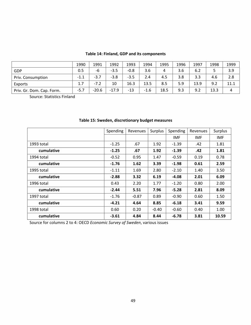
49 

 

   

Table 14: Finland, GDP and its components 

1990  1991  1992  1993  1994  1995  1996  1997  1998  1999 

GDP  0.5  ‐6  ‐3.5  ‐0.8  3.6  4  3.6  6.2  5  3.9 

Priv. Consumption  ‐1.1  ‐3.7  ‐3.8  ‐3.5  2.4  4.5  3.8  3.3  4.6  2.8 

Exports  1.7  ‐7.2  10  16.3  13.5  8.5  5.9  13.9  9.2  11.1 

Priv. Gr. Dom. Cap. Form.  ‐5.7  ‐20.6  ‐17.9  ‐13  ‐1.6  18.5  9.3  9.2  13.3  4 

Source: Statistics Finland 

 

Table 15: Sweden, discretionary budget measures 

   Spending  Revenues Surplus Spending  Revenues Surplus 

IMF  IMF  IMF 

1993 total  ‐1.25  .67  1.92  ‐1.39  .42  1.81 

         cumulative  ‐1.25  .67  1.92  ‐1.39  .42  1.81 

1994 total  ‐0.52  0.95  1.47  ‐0.59  0.19  0.78 

         cumulative  ‐1.76  1.62  3.39  ‐1.98  0.61  2.59 

1995 total  ‐1.11  1.69  2.80  ‐2.10  1.40  3.50 

         cumulative  ‐2.88  3.32  6.19  ‐4.08  2.01  6.09 

1996 total  0.43  2.20  1.77  ‐1.20  0.80  2.00 

         cumulative  ‐2.44  5.51  7.96  ‐5.28  2.81  8.09 

1997 total  ‐1.76  ‐0.87  0.89  ‐0.90  0.60  1.50 

         cumulative  ‐4.21  4.64  8.85  ‐6.18  3.41  9.59 

1998 total  0.60  0.20  ‐0.40  ‐0.60  0.40  1.00 

         cumulative  ‐3.61  4.84  8.44  ‐6.78  3.81  10.59 

Source for columns 2 to 4: OECD Economic Survey of Sweden, various issues 

    

50 

 

 

Table 16: Sweden, Interest rates 

  1990  1991  1992  1993  1994  1995  1996  1997  1998  1999 

Nom. long  13.2  10.7  10.0  8.6  9.7  10.3  8.1  6.7  5.0  5.0 

Nom. short  13.7  11.6  13.1  8.4  7.4  8.8  5.8  4.1  4.2  3.1 

Real long  2.8  1.3  7.6  3.8  7.6  7.8  7.5  6.0  5.3  4.5 

Real short  3.4  2.2  10.7  3.7  5.3  6.3  5.3  3.5  4.5  2.7 

Long – short  ‐0.5  ‐0.9  ‐3.1  0.2  2.3  1.5  2.2  2.5  0.8  1.9 

Long – long DEU  4.5  2.3  2.2  2.1  2.8  3.4  1.8  1.0  0.4  0.5 

Source: OECD Economic Outlook, No. 88; Long term interest rate for Germany until 1990: OECD Economic Outlook No. 72 

 

  

Table 17: Sweden, competitiveness indicators  

  

  

1990  1991  1992  1993  1994  1995  1996  1997  1998  1999 

hourly earnings in manuf.1   8.5  5.5  4.6  3.3  4.1  5.4  6.6  4.4  3.6  1.8 

ULC, total economy2  11.4  6.3  ‐0.1  0.3  0.9  0.1  4.7  0.5  0.3  ‐0.9 

ULC, manuf. 2  7.8  7.7  ‐0.5  ‐7.6  ‐7.2  ‐2.5  4.5  ‐4.4  ‐4.7  ‐6.8 

Nom. eff. exch. rate, chain‐linked2   0.4  0.9  2.4  ‐17.7  1.2  0.4  10.1  ‐3.3  ‐0.2  ‐0.3 

Relative ULC, manuf. 2  2.5  2.9  ‐2.7  ‐26.8  ‐6.4  ‐4.1  12.8  ‐7.2  ‐6.4  ‐7.0 

Real eff. exch. rate, nom. wages3  2.8  1.2  ‐1.4  ‐18.8  0.2  ‐1.1  13.6  ‐4.4  ‐3.4  ‐4.5 

Real eff.  exch. rate, ULC3   1.2  2.6  ‐1.5  ‐25.1  ‐6.7  ‐4.1  12.6  ‐7.5  ‐6.6  ‐9.5 

Labor prod. per person, all econ.1  1.1  0.4  2.1  5.4  5.3  3.1  2.6  4.4  2.4  2.5 

Labor prod.  per person, manuf. 1  2.0  0.5  5.2  10.1  15.5  7.0  3.7  9.3  6.6  9.7 

Labor prod. per hour, all econ. 1  1.4  1.3  1.0  4.3  2.8  2.8  1.8  4.1  2.5  2.0 

Labor prod.  per hour, manuf. 1  1.2  0.8  4.3  7.1  10.4  6.4  3.5  9.6  6.5  9.0 

CPI2  10.4  9.4  2.4  4.7  2.2  2.5  0.5  0.7  ‐0.3  0.5 

Notes: An increase in measures of nominal or real exchange rate is an appreciation. Sources: 1 OECD Main Economic Indicators; 2 OECD Economic Outlook No. 88; 3  EUROSTAT  

51 

 

  

 

 

Table 18: Sweden, GDP and its components 

 

1990  1991  1992  1993  1994  1995  1996  1997  1998  1999  2000 

GDP  1.0  ‐1.1  ‐1.2  ‐2.1  4.0  3.9  1.6  2.7  4.2  4.7  4.5 

Priv. Consumption  ‐0.5  0.9  ‐1.3  ‐3.6  2.1  1.1  1.8  2.8  3.3  4.0  5.3 

Exports  2.1  ‐1.9  2.0  8.3  13.5  11.3  4.4  13.8  9.0  7.2  11.7 

Gr. Dom. Cap. Form.  0.2  ‐8.5  ‐11.3  ‐14.6  7.0  9.9  4.7  0.6  8.8  8.7  5.7 

Mach. and Equipm.  ‐0.2  ‐12.0  ‐13.8  ‐14.4  25.1  23.7  7.5  3.5  9.7  6.3  1.7 

Dwellings  7.2  ‐2.4  ‐11.6  ‐33.5  ‐33.6  ‐23.5  8.9  ‐8.1  5.4  13.3  14.8 

Other Construction  ‐2.0  ‐5.9  ‐6.4  ‐2.1  13.9  11.4  ‐1.9  ‐6.2  2.6  ‐2.6  2.9 

Source: Statistics Sweden 

   

52 

 

References 

 

Ades, A., M. Kiguel, and N. Liviatan  (1993): “Exchange‐rate‐based stabilization: Tales  from Europe and 

Latin America”, World Bank Policy Research Working Paper WPS 1087 

Alesina, A. and S. Ardagna  (1998),  “Tales of Fiscal Adjustment,” Economic Policy, Vol. 13, No. 27, pp. 

487–545. 

Alesina, A. and S. Ardagna (2010):  “Large Changes in Fiscal Policy: Taxes versus Spending,” in: Tax Policy 

and the Economy, Vol. 24, ed. By Jeffrey R. Brown (Cambridge, Massachusetts: National .Bureau 

of Economic Research) 

Alesina, A. and R. Perotti  (1995):   “Fiscal Expansions and Adjustments  in OECD Economies”, Economic 

Policy, n.21, 207‐247. 

Alesina,  A.  and  R.  Perotti  (1997):  "Fiscal  Adjustments  In  OECD  Countries:  Composition  and 

Macroeconomic Effects," International Monetary Fund Staff Papers, v44(2,Jun), 210‐248. 

Alesina A., R. Perotti, and  J. Tavares  (1998): “The Political Economy of Fiscal Adjustments”, Brookings 

Papers on Economic Activity, Spring  

Andersen,  T.  and  O.  Risager  (1990):  “Wage  formation  in  Denmark“,  in  Calmfors,  L.  (ed.):    Wage 

formation and macroeconomic policies in Nordic countries, Oxford University Press 

Angrist, J. and J.S. Pischke (2008): Mostly Harmless Econometrics: An Empiricist’s Companion, Princeton 

University Press 

Baker, D. (2010): “The myth of expansionary fiscal austerity”, Center for Economic and Policy Research, 

Washington DC 

Barry, F.  (2000): “Convergence is not automatic: Lessons from Ireland for Central and Eastern Europe”, 

The World Economy, November 

Barry, F. and M. B. Devereux  (1995): “The expansionary fiscal contraction hypothesis: a neo‐keynesian 

analysis”, Oxford Economic Papers, 47,  249‐64 

Benetrix and P. R. Lane (011): “Financial Cycles and Fiscal Cycles”, mimeo, University College Dublin 

Bergman,  U. M.  and M. M.  Hutchinson  (2010):  “Expansionary  fiscal  contractions:  Re‐evaluating  the 

Danish case”, International Economic Journal, 24(1), 71‐93 

Bertrand, M., E. Duflo, and S. Mullainathan (2004): “How much should we trust difference‐in‐difference 

estimates?”, The Quarterly Journal of Economics, February, 249‐75 

Blanchard, O.J. and R. Perotti (2002): “An Empirical Characterization of the Dynamic Effects of Changes 

in Government Spending and Taxes on Output”, The Quarterly Journal of Economics, 1329‐1368. 

53 

 

Bradley,J.  and  K. Whelan  (1997):  “The  Irish  expansionary  fiscal  contraction:  a  tale  from  one  small 

European economy”, Economic Modelling, 14, 175‐201 

Broadbent, Ben, and Kevin Daly, 2010, “Limiting  the Fall‐Out  from Fiscal Adjustment,” Goldman Sachs 

Global Economics Paper No. 195 (New York: Goldman Sachs) 

Devries,P.,    J.  Guajardo,  D.  Leigh,  and  A.  Pescatori  (2011):  “A  new  action‐based  dataset  of  fiscal 

consolidations”, IMF  WP/11/128, at  

http://www.imf.org/external/pubs/cat/longres.aspx?sk=24892.0 

Dornbusch, R. (1989): “Ireland’s disinflation”, Economic Policy, April,  173‐201 

Drazen,  A.  (1990):  “discussion  of  Giavazzi  and  Pagano”,  in  Blanchard,  O.  and  S.  Fischer,  eds:  NBER 

Macroeconomics Annual 1990. Cambridge, Mass. and London:MIT Press, pp. 111‐115. 

Durkan, J. (1992): “Social consensus and incomes policy”, The Economic and Social Review, vol. 23, No. 3, 

347‐63 

Favero, C., F. Giavazzi, and J. Perego (2011): “Country heterogeneity and the  international evidence on 

fiscal policy”, mimeo, IGIER – Bocconi University 

Fedalino, A., A. Ivanova, and M. Horton (2009): “Computing cyclically adjusted balances and automatic 

stabilizers”,  International  Monetary  Fund  Technical  Notes  and  Manuals,  Fiscal  Affairs 

Department 

Giavazzi, F. and M. Pagano (1990):  “Can Severe Fiscal Contractions Be Expansionary? Tales of Two Small 

European Countries,” in Blanchard, O. and S. Fischer, eds: NBER Macroeconomics Annual 1990. 

Cambridge, Mass. and London:MIT Press, pp. 75‐111. 

Giavazzi,  F.  and M.  Pagano  (1996):    “Non‐Keynesian  Effects  of  Fiscal  Policy  Changes:  International 

Evidence and  the Swedish Experience,” Swedish Economic Policy Review, Vol. 3, No. 1, pp.67–

103. 

Guichard, S., M. Kennedy, E. Wurzel, and   C. André (2007): “What promotes fiscal consolidation: OECD 

country experiences”, OECD Economic Department working paper ECO/WKP(2007)13 

Hardy,  P.,  L.  Kamener,  and  L.  Karotie  (2011):  “European  fiscal  consolidations:  four  factors  that will 

support success”, The Boston Consulting Group 

Hauptmeier S., Heipertz M. and L. Schuknecht (2007): “Expenditure Reform in Industrialized Countries: A 

Case Study Approach”, Fiscal Studies, vol. 28, no. 3, pp. 293–342. 

Henriksson, J. (2007): “Ten lessons about budget consolidations” The Bruegel Essay and Lecture Series 

Honkapohja,  S.  and  E.  Koskela  (1999):  “The  economic  crisis  in  the  1990s  in  Finland”,  The  Research 

Institute of the Finnish Economy, Discussion paper No. 683  

54 

 

Honohan, P. (1989): “Comments to Dornbusch”, Economic Policy, April,  202‐205 

Honohan, P. and B. Walsh  (2002):  “Catching up with  the  leaders:  the  Irish hare”, Brookings Panel on 

Economic Activity, I, 1‐57 

International Monetary  Fund  (2010):  “Will  it  hurt? Macroeconomic  effects  of  fiscal  consolidations”, 

Chapter 3 of The World Economic Outlook, October 

Jayadev, A. and M. Konczal  (2010): “The boom not  the slump:  the  right  time  for  fiscal austerity”, The 

Roosevelt Institute 

Jonung, L., J. Kiander, and P. Vartia (2008): „The great financial crisis in Finland and Sweden”, Economic 

Paper, DG ECFIN 

Krugman,  P.  (2010):  “Myths  of  austerity”,  The  New  York  Times,  July  1,  2010,  at 

http://www.nytimes.com/2010/07/02/opinion/02krugman.html?ref=paulkrugman 

Krugman,  P.  (2011):  “When  austerity  fails”,  The  New  York  Times,  May  22,  2011,  at 

http://www.nytimes.com/2011/05/23/opinion/23krugman.html?ref=paulkrugman 

Lane, P. R. (2000): “Disinflation, Switching Nominal Anchors and Twin Crises: the Irish Experience”, Policy 

Reform, Vol. 3,  301‐326 

Lassen, D. (2010): “Fiscal consolidations in advanced industrialized democracies: economics, politics, and 

governance”, Rapport till Finanspolitiska radet 2010/4, University of Copenhagen  

Lilico, A., E. Holmes and H. Samen (2009): “Controlling spending and government deficits: Lessons from 

history and international experience”,Policy Exchange  

Ljungman, G.  (2008):  “Expenditure  ceilings  –  a  survey”,  International Monetary  Fund Working  Paper 

WP/08/282 

McAleese, D. (1990): “Ireland’s  economic recovery”, Irish Banking Review, Summer, 18‐32 

McCarthy, C. (2010): “Ireland’s second round of cuts: a comparison with the last time”, in: Springford, J.: 

Dealing with debt: lessons from abroad, CentreForum Canada, Ernst & Young,  41‐54  

Morris,  R.  and  L.  Schuknecht  (2007):  “Structural  Balances  and  Revenue Windfalls:  the  Role  of  Asset 

Prices Revisited,” European Central Bank Working Paper Series No. 737. 

Ramey,  V.A.  (2011):  “Identifying Government  Spending  Shocks:  It's All  in  the  Timing”,  The Quarterly 

Journal of Economics 

Rigobon, R. and T. Stoker (2005): “Censored Regressors and Expansion Bias”, mimeo, MIT  

Romer, C. and D. Romer  (2010):    “The Macroeconomic Effects of Tax Changes: Estimates Based on a 

New Measure of Fiscal Shocks,” American Economic Review, Vol. 100, No. 3, pp. 763‐801. 

55 

 

Walsh,  B,  (1993):  “Credibility,  Interest  Rates  and  the  ERM:  The  Irish  Experience”, Oxford  Bulletin  of 

Economics and Statistics, 55, issue 4, p. 439‐52 

Whelan,  K.  (2010):  “The  enduring  influence  of  Ireland’s  1987  adjustment”,  Irish  Economy  blog, 

http://www.irisheconomy.ie/index.php/2010/08/20/the‐enduring‐influence‐of‐irelands‐1987‐

adjustment/ 

Wolswijk, G.  (2007):    “Short‐  and  Long‐Run  Tax  Elasticities—the Case of  the Netherlands,”  European 

Central Bank Working Paper Series No. 763 (Frankfurt: European Central Bank). 

   

56 

 

 

Figure 1: The censoring bias of the IMF approach 

  

  

   

57 

 

 

  

Figure 2: Finland, consumer confidence