the apl-uw multiport acoustic projector system
TRANSCRIPT
Applied Physics Laboratory University of Washington1013 NE 40th Street Seattle, Washington 98105-6698
The APL-UW Multiport Acoustic Projector System
Technical Report
APL-UW TR 0902December 2009
Approved for public release; distribution is unlimited.
by Rex K. Andrew
N00014-03-1-0181, N00014-07-1-0743, and N00014-08-1-0843

UNIVERSITY OF WASHINGTON • APPLIED PHYSICS LABORATORY
ACKNOWLEDGMENTS
Thanks are extended to Dr. Jack Butler of ImageAcoustics, Inc., who contributed help-ful discussions during the development of the first tuner; Mr. Jan Lindberg of the NavalUndersea Warfare Center Newport for the loan of the MP200/TR1446; and Dr. Jim Mercerof APL-UW who negotiated to borrow the MP200/TR1446for APL-UW. This develop-ment effort was funded under ONR Grants N00014-03-1-0181, N00014-07-1-0743, andN00014-08-1-0843.
ii TR 0902
UNIVERSITY OF WASHINGTON • APPLIED PHYSICS LABORATORY
ABSTRACT
The Applied Physics Laboratory of the University of Washington (APL-UW) acquiredon loan an experimental device known as the multiport transducer. APL-UW developed, inturn, a complete transmitter system that integrates this transducer, capable of wideband op-eration (roughly 180–350 Hz) from near-surface depths to depths greater than 1000 m. Thesystem’s electrical components include an autotransformer tuner, a battery power module,and a fibre optic telemetry interface; mechanical components include a steel supportingstructure and a pressure-compensated tuner housing; an additional acoustical componentis a monitor hydrophone in a vibration isolation mount; and asignal component involvesa lumped parameter SPICE circuit model approximation of theentire end-to-end system,an associated C++ application to predict the time-domain acoustic far field from a standardtime-domain waveform input file, and a pre-equalization filter. The multiport system was akey element in a 2009 at-sea ocean acoustics experiment located in the Philippine Sea andprovided many hours of high-quality pulsed transmissions to a nearby vertical line array ofhydrophones.
TR 0902 iii

UNIVERSITY OF WASHINGTON • APPLIED PHYSICS LABORATORY
Contents
1 Introduction 1
2 The Multiport Transducer 2
2.1 Introduction . . . . . . . . . . . . . . . . . . . . . . . . . . . . . . . . . . 2
2.2 Equivalent Electrical Circuit — Theory . . . . . . . . . . . . . .. . . . . 3
2.3 2006 Lake Washington Test Configuration . . . . . . . . . . . . . .. . . . 5
2.4 Equivalent Circuit Characterization — Results . . . . . . .. . . . . . . . . 5
2.5 Electro-Acoustic Transformation Ratio . . . . . . . . . . . . .. . . . . . . 8
2.5.1 The Parameterka . . . . . . . . . . . . . . . . . . . . . . . . . . . 13
2.5.2 Current Divider Factor . . . . . . . . . . . . . . . . . . . . . . . . 14
2.5.3 Field Point Range . . . . . . . . . . . . . . . . . . . . . . . . . . . 14
2.5.4 Field Pressure . . . . . . . . . . . . . . . . . . . . . . . . . . . . . 14
2.5.5 Drive Current . . . . . . . . . . . . . . . . . . . . . . . . . . . . . 16
2.5.6 Incorporating the Transformation Ratio . . . . . . . . . . .. . . . 16
3 Tuning 19
3.1 Single Resonance Theory . . . . . . . . . . . . . . . . . . . . . . . . . . .19
3.2 Multiple Resonance Theory and Wideband Signals . . . . . . .. . . . . . 19
3.3 The 1:2 Tuner . . . . . . . . . . . . . . . . . . . . . . . . . . . . . . . . . 22
3.4 The 1:3 Tuner . . . . . . . . . . . . . . . . . . . . . . . . . . . . . . . . . 26
4 The Multiport System 32
5 System Model 39
5.1 Introduction . . . . . . . . . . . . . . . . . . . . . . . . . . . . . . . . . . 39
iv TR 0902
UNIVERSITY OF WASHINGTON • APPLIED PHYSICS LABORATORY
5.1.1 D/A Converter . . . . . . . . . . . . . . . . . . . . . . . . . . . . 39
5.1.2 Power Amplifier . . . . . . . . . . . . . . . . . . . . . . . . . . . 40
5.1.3 Low-Pass Filter . . . . . . . . . . . . . . . . . . . . . . . . . . . . 40
5.1.4 Cable . . . . . . . . . . . . . . . . . . . . . . . . . . . . . . . . . 41
5.2 Acoustic Radiation: the “Double Doublet” Model . . . . . . .. . . . . . . 41
5.3 Model Implementation . . . . . . . . . . . . . . . . . . . . . . . . . . . . 42
5.4 Performance Validation . . . . . . . . . . . . . . . . . . . . . . . . . . .. 43
5.4.1 Broadband Beampattern . . . . . . . . . . . . . . . . . . . . . . . 43
5.4.2 Transmit Response . . . . . . . . . . . . . . . . . . . . . . . . . . 45
5.4.3 Broadside to Monitor Hydrophone Scaling . . . . . . . . . . .. . 46
6 Signal Equalization 47
6.1 Introduction . . . . . . . . . . . . . . . . . . . . . . . . . . . . . . . . . . 47
6.2 Theory . . . . . . . . . . . . . . . . . . . . . . . . . . . . . . . . . . . . . 49
6.3 In-water Tests . . . . . . . . . . . . . . . . . . . . . . . . . . . . . . . . . 53
6.4 Summary . . . . . . . . . . . . . . . . . . . . . . . . . . . . . . . . . . . 53
7 The Philippine Sea Engineering Test / Pilot Study 56
7.1 Summary . . . . . . . . . . . . . . . . . . . . . . . . . . . . . . . . . . . 56
7.2 System Limitations . . . . . . . . . . . . . . . . . . . . . . . . . . . . . . 58
7.3 Lessons Learned . . . . . . . . . . . . . . . . . . . . . . . . . . . . . . . 62
References 65
A 2006 Lake Washington Test Results A1
B System SPICE Netlist B1
TR 0902 v

UNIVERSITY OF WASHINGTON • APPLIED PHYSICS LABORATORY
C 2009 Philippine Sea Transmissions C1
C.1 Background . . . . . . . . . . . . . . . . . . . . . . . . . . . . . . . . . . C1
C.2 Station SS45 . . . . . . . . . . . . . . . . . . . . . . . . . . . . . . . . . . C1
C.3 Station SS107 . . . . . . . . . . . . . . . . . . . . . . . . . . . . . . . . . C3
List of Figures
1 The MP200/TR1446. . . . . . . . . . . . . . . . . . . . . . . . . . . . . . 2
2 Simple equivalent electrical circuit for the Multiport Source. . . . . . . . . 3
3 B(ω)/ω versus frequency, 2006 Lake Washington test. . . . . . . . . . . . 6
4 Fourier transforms of drive signals, 2006 Lake Washingtontest. . . . . . . 7
5 Admittance locus, SPICE simulation. . . . . . . . . . . . . . . . . . .. . 8
6 Electro-acoustic transformation element. . . . . . . . . . . . .. . . . . . . 11
7 The modified equivalent circuit involving transformationelement. . . . . . 11
8 Acoustic doublet. . . . . . . . . . . . . . . . . . . . . . . . . . . . . . . . 13
9 An estimated monitor hydrophone autospectrum, 2006 Lake Washingtontest. . . . . . . . . . . . . . . . . . . . . . . . . . . . . . . . . . . . . . . 15
10 An estimated drive current autospectrum, 2006 Lake Washington test. . . . 16
11 SPICE representation of an ideal transformer. . . . . . . . . .. . . . . . . 17
12 The SPICE circuit corresponding to the circuit of Fig. 7. .. . . . . . . . . 18
13 Tuning example circuit. . . . . . . . . . . . . . . . . . . . . . . . . . . . .20
14 Admittance loops for the single resonance circuit, with and without thetuning inductor. . . . . . . . . . . . . . . . . . . . . . . . . . . . . . . . . 21
15 Simple electrical equivalent SPICE model of transducer with a parallel tun-ing inductor. . . . . . . . . . . . . . . . . . . . . . . . . . . . . . . . . . . 21
16 Conductance and susceptance of the circuit, no tuning inductor. . . . . . . . 23
vi TR 0902
UNIVERSITY OF WASHINGTON • APPLIED PHYSICS LABORATORY
17 Conductance and susceptance of the tuned circuit. . . . . . .. . . . . . . . 23
18 Corner view of the first tuner. . . . . . . . . . . . . . . . . . . . . . . . .24
19 End view of the first tuner. . . . . . . . . . . . . . . . . . . . . . . . . . . 24
20 Housing for the tuner. . . . . . . . . . . . . . . . . . . . . . . . . . . . . 25
21 Top view looking inside the tuner housing. . . . . . . . . . . . . .. . . . 25
22 Tuner and housing completely assembled. . . . . . . . . . . . . . .. . . . 26
23 Simple electrical equivalent SPICE circuit involving the autotransformer. . 27
24 Admittance loop, tuned for the lower (212 Hz) resonance frequency. . . . . 29
25 Admittance loop, tuned between the resonances. . . . . . . . .. . . . . . 29
26 Admittance loop, tuned for the upper (320 Hz) resonance frequency. . . . . 29
27 Conductance and susceptance curves, tuned for the lower (212 Hz) reso-nance frequency. . . . . . . . . . . . . . . . . . . . . . . . . . . . . . . . 30
28 Conductance and susceptance curves, tuned between the resonances. . . . 30
29 Conductance and susceptance curves, tuned for the upper (320 Hz) reso-nance frequency. . . . . . . . . . . . . . . . . . . . . . . . . . . . . . . . 30
30 Tuner voltage across the secondary. The input voltage wasunity. Circuittuned for the lower (212 Hz) resonance frequency. . . . . . . . . .. . . . 31
31 Voltage across the secondary. The input voltage was unity. Circuit tunedbetween the resonances. . . . . . . . . . . . . . . . . . . . . . . . . . . . 31
32 Voltage across the secondary. The input voltage was unity. Circuit tunedfor the upper (320 Hz) resonance frequency. . . . . . . . . . . . . . .. . 31
33 Block diagram of essential components for the complete multiport system. 32
34 Schematic of the initial mechanical configuration. . . . . .. . . . . . . . . 33
35 Engineering drawings, MP200/TR1446 assembly. . . . . . . . .. . . . . 35
36 System fully assembled on the deck of the M/VSeaHorse, 2009 LakeWashington test. . . . . . . . . . . . . . . . . . . . . . . . . . . . . . . . 36
37 Deck preparations, 2009 Lake Washington test. . . . . . . . . .. . . . . . 37
TR 0902 vii
UNIVERSITY OF WASHINGTON • APPLIED PHYSICS LABORATORY
38 Deployment from the M/VSeaHorse, 2009 Lake Washington test. . . . . . 38
39 Block diagram of the entire system. . . . . . . . . . . . . . . . . . . .. . 39
40 SPICE model for an ideal D/A converter. . . . . . . . . . . . . . . . .. . . 40
41 Circuit model for the low-pass filter. . . . . . . . . . . . . . . . . .. . . . 41
42 Circuit model for the cable. . . . . . . . . . . . . . . . . . . . . . . . . .42
43 Geometry for the acoustic field computation. . . . . . . . . . . .. . . . . . 44
44 Theoretical broadband beampattern. . . . . . . . . . . . . . . . . .. . . . 44
45 Theoretical transmit response. . . . . . . . . . . . . . . . . . . . . .. . . 45
46 The Massa equalizer disassembled. . . . . . . . . . . . . . . . . . . .. . . 47
47 Magnitude response of Massa equalizer. . . . . . . . . . . . . . . .. . . . 48
48 Phase response of Massa equalizer. . . . . . . . . . . . . . . . . . . .. . . 48
49 Schematic block diagram involving the Massa equalizer. .. . . . . . . . . 48
50 Signal flow diagram for a post-processing equalizer filter. . . . . . . . . . . 50
51 Similar to Fig. 50, but with the equalizer filter placed before the D/A con-verter. . . . . . . . . . . . . . . . . . . . . . . . . . . . . . . . . . . . . . 51
52 Off-line implementation of pre-equalization, based on Fig. 51. . . . . . . . 51
53 Equalizer transfer function, fileeq01.nc . . . . . . . . . . . . . . . . . . 51
54 Simulated pulse-compressed output with and without equalization. . . . . . 52
55 Pulse compressed noise signatures, 2009 Lake Washingtontest. . . . . . . 53
56 Real and simulated radiated spectra, 2009 Lake Washington test. . . . . . . 54
57 Geographical context for the Philippine Sea 2009 exercise. . . . . . . . . . 57
58 Dockside mobilization, Kao-Hsiung harbor, April 2009. .. . . . . . . . . . 58
59 The MP200/TR1446 on the fantail of the R/VMelville. . . . . . . . . . . . 59
60 Deploying the MP200/TR1446. . . . . . . . . . . . . . . . . . . . . . . . .60
61 The MP200/TR1446 descending into the sea. . . . . . . . . . . . . .. . . 60
viii TR 0902
UNIVERSITY OF WASHINGTON • APPLIED PHYSICS LABORATORY
62 Recovering the MP200/TR1446. . . . . . . . . . . . . . . . . . . . . . . .61
63 Attaching the monitor hydrophone to the suspension cable. . . . . . . . . . 61
64 Pulse-compressed result, transmission file1239933870.sam, as mea-sured on the monitor hydrophone. . . . . . . . . . . . . . . . . . . . . . . 63
65 2006 Lake Washington admittance loop, fileMPTEST01.DAT . . . . . . . A2
66 2006 Lake Washington admittance loop, fileMPTEST02.DAT . . . . . . . A3
67 2006 Lake Washington admittance loop, fileMPTEST03.DAT . . . . . . . A4
68 2006 Lake Washington admittance loop, fileMPTEST04.DAT . . . . . . . A5
69 2006 Lake Washington admittance loop, fileMPTEST05.DAT . . . . . . . A6
70 2006 Lake Washington admittance loop, fileMPTEST06.DAT . . . . . . . A7
71 2006 Lake Washington admittance loop, fileMPTEST07.DAT . . . . . . . A8
72 2006 Lake Washington admittance loop, fileMPTEST08.DAT . . . . . . . A9
73 2006 Lake Washington admittance loop, fileMPTEST11.DAT . . . . . . . A10
74 2006 Lake Washington admittance loop, fileMPTEST12.DAT . . . . . . . A11
75 2006 Lake Washington admittance loop, fileMPTEST13.DAT . . . . . . . A12
76 2006 Lake Washington admittance loop, fileMPTEST14.DAT . . . . . . . A13
77 2006 Lake Washington admittance loop, fileMPTEST15.DAT . . . . . . . A14
78 2006 Lake Washington admittance loop, fileMPTEST16.DAT . . . . . . . A15
List of Tables
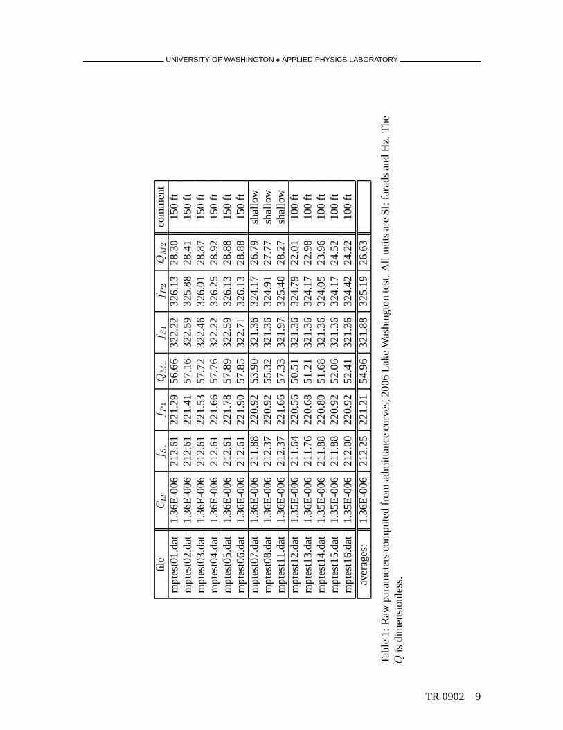
1 Raw parameters computed from admittance curves, 2006 LakeWashingtontest. . . . . . . . . . . . . . . . . . . . . . . . . . . . . . . . . . . . . . . 9
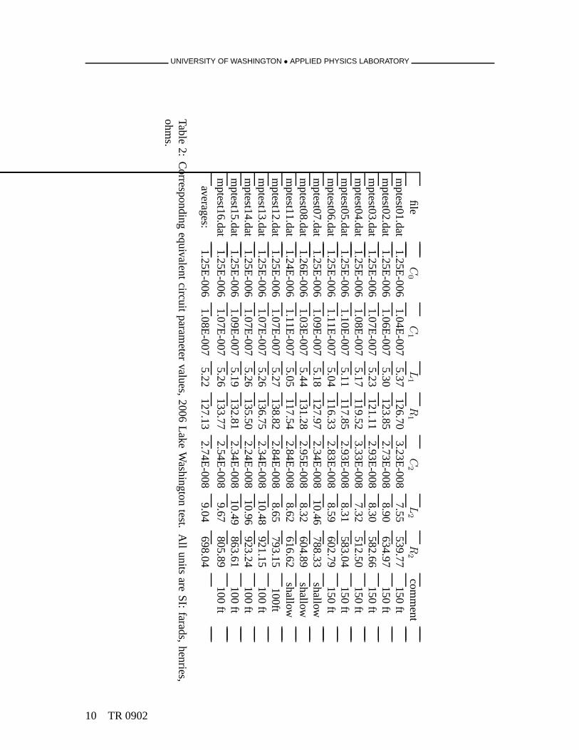
2 Corresponding equivalent circuit parameter values, 2006Lake Washingtontest. . . . . . . . . . . . . . . . . . . . . . . . . . . . . . . . . . . . . . . 10
3 Values ofka for both tubes. . . . . . . . . . . . . . . . . . . . . . . . . . 14
TR 0902 ix
UNIVERSITY OF WASHINGTON • APPLIED PHYSICS LABORATORY
4 Slant ranges from transducer to monitor hydrophone, 2006 Lake Washing-ton test. . . . . . . . . . . . . . . . . . . . . . . . . . . . . . . . . . . . . 14
5 Radiated pressure and drive current magnitudes from the 2006 Lake Wash-ington test. . . . . . . . . . . . . . . . . . . . . . . . . . . . . . . . . . . . 15
6 Transformation ratios calculated from the 2006 Lake Washington data. . . . 16
7 Lumped acoustical equivalent circuit values for the resonant branch com-ponents. . . . . . . . . . . . . . . . . . . . . . . . . . . . . . . . . . . . . 17
8 “Broadband power factor” for the circuit of Fig. 15 and an m-sequencedrive signal. . . . . . . . . . . . . . . . . . . . . . . . . . . . . . . . . . . 22
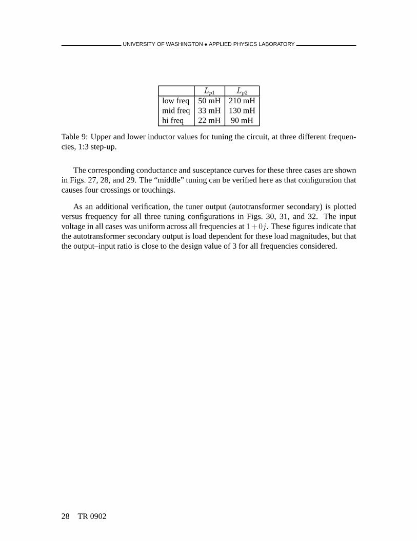
9 Upper and lower inductor values for tuning the circuit, at three differentfrequencies, 1:3 step-up. . . . . . . . . . . . . . . . . . . . . . . . . . . . 28
10 Input and output measurements for a 300-Hz sine wave, Instruments, Inc.,L50 power amplifier. . . . . . . . . . . . . . . . . . . . . . . . . . . . . . 40
11 Circuit parameters for the low pass filter model. . . . . . . . .. . . . . . . 41
12 Circuit parameters for the electro-opto-mechanical cable. . . . . . . . . . . 41
13 AT-GPIB commands for retrieving trace data from the HP3589A. . . . . . . 49
14 Summary of transmission collections, Lake Washington 2006 test. . . . . . A1
15 Signal parameters, 2009 Philippine Sea experiment. . . . .. . . . . . . . . C2
16 Multiport transmissions for station SS45, 2009 Philippine Sea experiment. . C2
17 Multiport transmissions for station SS107, 2009 Philippine Sea experiment. C4
x TR 0902
UNIVERSITY OF WASHINGTON • APPLIED PHYSICS LABORATORY
EXECUTIVE SUMMARY
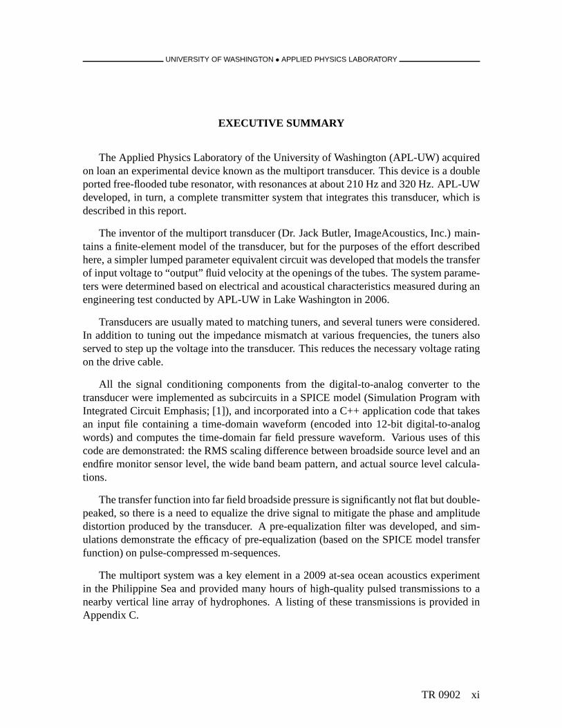
The Applied Physics Laboratory of the University of Washington (APL-UW) acquiredon loan an experimental device known as the multiport transducer. This device is a doubleported free-flooded tube resonator, with resonances at about 210 Hz and 320 Hz. APL-UWdeveloped, in turn, a complete transmitter system that integrates this transducer, which isdescribed in this report.
The inventor of the multiport transducer (Dr. Jack Butler, ImageAcoustics, Inc.) main-tains a finite-element model of the transducer, but for the purposes of the effort describedhere, a simpler lumped parameter equivalent circuit was developed that models the transferof input voltage to “output” fluid velocity at the openings ofthe tubes. The system parame-ters were determined based on electrical and acoustical characteristics measured during anengineering test conducted by APL-UW in Lake Washington in 2006.
Transducers are usually mated to matching tuners, and several tuners were considered.In addition to tuning out the impedance mismatch at various frequencies, the tuners alsoserved to step up the voltage into the transducer. This reduces the necessary voltage ratingon the drive cable.
All the signal conditioning components from the digital-to-analog converter to thetransducer were implemented as subcircuits in a SPICE model(Simulation Program withIntegrated Circuit Emphasis; [1]), and incorporated into aC++ application code that takesan input file containing a time-domain waveform (encoded into 12-bit digital-to-analogwords) and computes the time-domain far field pressure waveform. Various uses of thiscode are demonstrated: the RMS scaling difference between broadside source level and anendfire monitor sensor level, the wide band beam pattern, andactual source level calcula-tions.
The transfer function into far field broadside pressure is significantly not flat but double-peaked, so there is a need to equalize the drive signal to mitigate the phase and amplitudedistortion produced by the transducer. A pre-equalizationfilter was developed, and sim-ulations demonstrate the efficacy of pre-equalization (based on the SPICE model transferfunction) on pulse-compressed m-sequences.
The multiport system was a key element in a 2009 at-sea ocean acoustics experimentin the Philippine Sea and provided many hours of high-quality pulsed transmissions to anearby vertical line array of hydrophones. A listing of these transmissions is provided inAppendix C.
TR 0902 xi

UNIVERSITY OF WASHINGTON • APPLIED PHYSICS LABORATORY
xii TR 0902
UNIVERSITY OF WASHINGTON • APPLIED PHYSICS LABORATORY
1 Introduction
In 2005 the Applied Physics Laboratory of the University of Washington (APL-UW) ac-quired on loan an experimental device known as the “multiport” transducer from the NavalUndersea Warfare Center Division Newport. This transducerwas originally designed andconstructed by ImageAcoustics, Inc. [Cohasset, MA] and Massa Products, Inc. [Hingham,MA] under a Small Business Innovative Research (SBIR) grantto ImageAcoustics, Inc.from the Naval Undersea Warfare Center Division Newport.
APL-UW was subsequently funded by Code 321OA of the Office of Naval Research(ONR) to develop a deep-water ship-suspended system based around the MP200/TR1446for operations in the ONR-sponsored Philippine Sea experiments of 2009 and 2010. Thisreport summarizes that development effort. Section 2 describes the development effort fora simple circuit model suitable for routine system performance calculations. Some of theseresults have been disseminated in previous notes; the calculations regarding the transfor-mation ratio are new. Chapter 3 describes the efforts made todesign and build a tuner forthe transducer. Section 4 describes the entire multiport system as built and deployed byAPL-UW. Section 5 describes an entire system model of the multiport system, includingthe top-side electronics and the electro-opto-mechanicalsuspension cable, and the prop-agator to predict the far field time-domain radiated acoustic pressure. This model wasincorporated for ease of use into a simulator code that takesas input a time-domain “drive”waveform in convenient standard.wav file format. Section 6 discusses the implementationof two different equalizers, necessary to compensate for the considerably non-flat responseof the transducer itself. Finally, section 7 provides a review of the system in use during anat-sea deployment on an acoustics experiment in the Philippine Sea in 2009.
TR 0902 1
UNIVERSITY OF WASHINGTON • APPLIED PHYSICS LABORATORY
2 The Multiport Transducer
2.1 Introduction
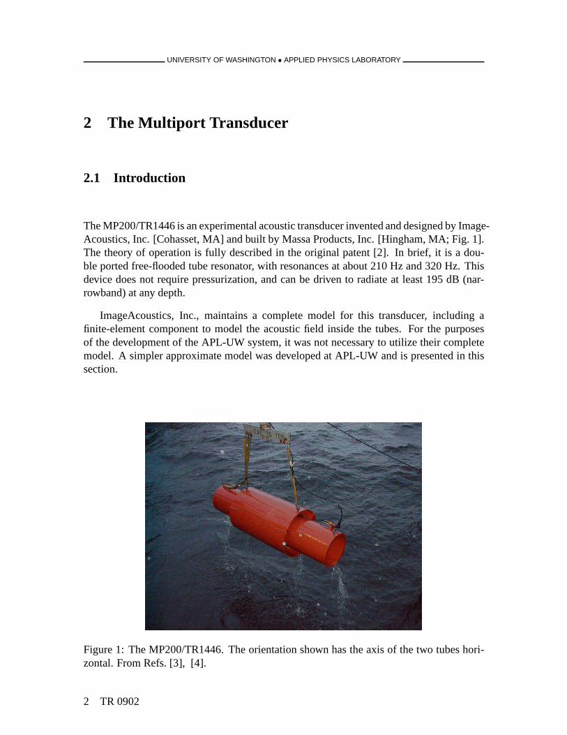
The MP200/TR1446 is an experimental acoustic transducer invented and designed by Image-Acoustics, Inc. [Cohasset, MA] and built by Massa Products,Inc. [Hingham, MA; Fig. 1].The theory of operation is fully described in the original patent [2]. In brief, it is a dou-ble ported free-flooded tube resonator, with resonances at about 210 Hz and 320 Hz. Thisdevice does not require pressurization, and can be driven toradiate at least 195 dB (nar-rowband) at any depth.
ImageAcoustics, Inc., maintains a complete model for this transducer, including afinite-element component to model the acoustic field inside the tubes. For the purposesof the development of the APL-UW system, it was not necessaryto utilize their completemodel. A simpler approximate model was developed at APL-UW and is presented in thissection.
Figure 1: The MP200/TR1446. The orientation shown has the axis of the two tubes hori-zontal. From Refs. [3], [4].
2 TR 0902

UNIVERSITY OF WASHINGTON • APPLIED PHYSICS LABORATORY
iRAD
i 0
L1 L2
C1 C2
R1 R2
C0
+
_
i
Figure 2: Simple equivalent electrical circuit for the Multiport Source. The “currents”i, i0andiRAD are defined in section 2.5.
2.2 Equivalent Electrical Circuit — Theory
Characterization of the equivalent electrical circuit parameters follows the procedures ofWilson [5], Stansfield [6], and Sherman and Butler [7]. Givena power amplifier drivevoltage ofv(t) with Fourier transformV (f) and a drive currenti(t) with Fourier transformI(f), the admittance is
Y (f) =I(f)
V (f)= G(f) + jB(f) (1)
whereG(f) is the conductance andB(f) is the susceptance, both in units of siemens, andj =
√−1. The curvesG(f), B(f) and the admittance locusY (f) can be used to determine
various “raw” parameters, as described below, which are then converted to the elements ofa simple equivalent circuit.
A simple but adequate equivalent circuit diagram (Fig. 2) represents the blocked capac-itance of the device with a shunt capacitor, and the two tubesof the device with two parallelseries RLC branches. There are two distinct resonances in the device, each represented byan RLC branch (Fig. 2), and these are far enough apart in frequency space that a sepa-rate analysis is pursued for each. The raw parameters and their computation are describedbelow:
Low-Frequency Capacitance.The effective input admittance at low frequency goes asB(ω)/ω asω goes to zero and is represented by the capacitanceCLF.
Motional Resonance.The motional resonance frequencyfS is determined by locating thepeak in the conductanceG(f).
TR 0902 3

UNIVERSITY OF WASHINGTON • APPLIED PHYSICS LABORATORY
Mechanical Q. The mechanical Q, denotedQM , is determined by the equation
QM =f0
f2 − f1
(2)
wheref0 is a resonance frequency, and(f1, f2) are the frequencies where the conduc-tance drops to half its maximum value at the resonance peak. These half-amplitudefrequencies were calculated using linear (inverse) interpolation aboutG = 0.5.
Parallel Resonance.The parallel resonance frequencyfP is determined by finding thefrequencyfP > fS where theY (f) locus meets the line from the origin to the point(G(fS), B(fS)) in the admittance plane.
Once these parameters have been determined, the following circuit parameters can becalculated:
Coupling Coefficient. The (squared) coupling coefficient is
k2 = 1 − f 2S
f 2P
(3)
Mechanical Capacitance.The effective resonator mechanical capacitance, denoted by C,is roughly
C = k2CLF (4)
Resonance Inductance.The effective resonator mechanical inductanceL is then relatedto C via the resonance frequency:
L =1
ω2SC
(5)
Blocked Capacitance.The blocked admittance is assumed here to be purely capacitative,and the capacitance is
C0 = CLF − C (6)
Resonance Resistance.The resistance at resonanceR is given roughly by
R =1
ωSCQM(7)
4 TR 0902

UNIVERSITY OF WASHINGTON • APPLIED PHYSICS LABORATORY
2.3 2006 Lake Washington Test Configuration
APL-UW tested the MP200/TR1446 over the side of the R/VHendersonfor several days inApril 2006 in Lake Washington. The transducer was driven by an 80486 computer runningMS-DOS and the programatocsam. The drive signal from the computer was routed toa Ling power amplifier and via the suspension cable to the transducer. A custom circuitinternal to the Ling monitors the “top-of-the-cable” drivevoltage and current.
An ITC 6050C hydrophone was deployed over the side of the R/VHendersonto moni-tor any acoustic emissions from the transducer. The hydrophone signal was routed into the“Tennelec” amplifier box (approximately no gain) through a Krohn–Hite filter (dialed topass 100 Hz to 400 Hz at 0 dB), through an HP 4436A attenuator (set to 0 dB attenuation),and then into the “bare” signal input on the card cage chassis.
The input signal was generated via the applicationseqsam and consisted of an m-sequence with octal law 2033. The modulation angle was 88.2092, 2 cycles per digit,1023 digits. The carrier frequency was 250 Hz. As is customary with ATOC (acousticthermometry of ocean climate) signals, the waveform was oversampled by a factor of 32,so the sampling rate of the playback digital–analog board was 8 kHz.
The programatocsam also performs simultaneous analog-to-digital while stream-ing out through the digital-to-analog (D/A) converter subsystem. In normal operation,five channels are captured: the 1 pulse/second line, power amplifier drive voltage moni-tor, power amplifier drive current monitor, “bare” acousticinput, and IRIG-M. Due to thehigh sampling rate, it was not possible to capture all five channels, and perform D/A, withthe computer power available. Therefore, only three channels were captured: the voltagemonitor, the current monitor, and the bare acoustic line.
Each test measurement was 120 s in duration. The programmable anti-alias filters onthe filter/gain card were set to 384 Hz automatically byatocsam.
2.4 Equivalent Circuit Characterization — Results
With the Ling power amplifier, the voltage monitor circuit divides the power amplifier drivevoltage by a factor of 1000, and the current monitor circuit converts the power amplifierdrive current to a voltage by 200 mV/A.
In practice,V (f) andI(f) are computed using discrete Fourier transforms. In regionsoutside the main band of the signal, these terms are largely noise, and therefore only theadmittance over the main frequency bandf ∈ [fmin, fmax] need be considered.
TR 0902 5
UNIVERSITY OF WASHINGTON • APPLIED PHYSICS LABORATORY
50 100 150 200 250 300 350 400 450−2
−1
0
1
2
3
4
5x 10
−6
frequency [Hz]
capacitance [farads]
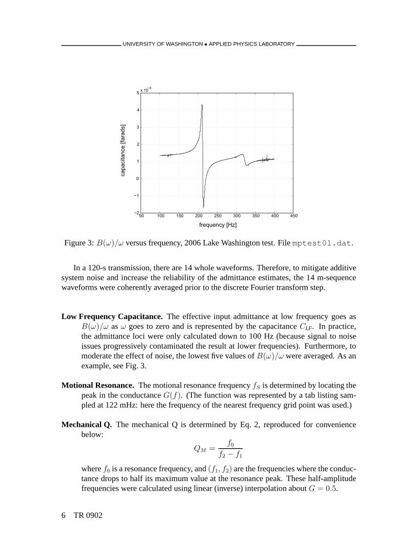
Figure 3:B(ω)/ω versus frequency, 2006 Lake Washington test. Filemptest01.dat.
In a 120-s transmission, there are 14 whole waveforms. Therefore, to mitigate additivesystem noise and increase the reliability of the admittanceestimates, the 14 m-sequencewaveforms were coherently averaged prior to the discrete Fourier transform step.
Low Frequency Capacitance.The effective input admittance at low frequency goes asB(ω)/ω asω goes to zero and is represented by the capacitanceCLF. In practice,the admittance loci were only calculated down to 100 Hz (because signal to noiseissues progressively contaminated the result at lower frequencies). Furthermore, tomoderate the effect of noise, the lowest five values ofB(ω)/ω were averaged. As anexample, see Fig. 3.
Motional Resonance.The motional resonance frequencyfS is determined by locating thepeak in the conductanceG(f). (The function was represented by a tab listing sam-pled at 122 mHz: here the frequency of the nearest frequency grid point was used.)
Mechanical Q. The mechanical Q is determined by Eq. 2, reproduced for conveniencebelow:
QM =f0
f2 − f1
wheref0 is a resonance frequency, and(f1, f2) are the frequencies where the conduc-tance drops to half its maximum value at the resonance peak. These half-amplitudefrequencies were calculated using linear (inverse) interpolation aboutG = 0.5.
6 TR 0902

UNIVERSITY OF WASHINGTON • APPLIED PHYSICS LABORATORY
0 50 100 150 200 250 300 350 400 450 5000
0.5
1
1.5
2x 10
6
0 50 100 150 200 250 300 350 400 450 5000
0.5
1
1.5
2x 10
5
0 50 100 150 200 250 300 350 400 450 5000
50
100
150
200
frequency [Hz]
Figure 4: Fourier transforms of drive signals, 2006 Lake Washington test. Top: drive signalfrom filemp001.sam. Middle: power amplifier drive voltage from filemptest15.sam.Bottom: P.A. drive current from filemptest15.sam. The middle and bottom panelsutilize the first m-sequence in the file.
The Fourier transforms of the drive signal and the voltage and current monitor channelsfor one m-sequence are shown in Fig. 4. The MP200/TR1446 has two resonances at ap-proximately 200 and 300 Hz. Note that there is a smoothing filter after the D/A prior to theLing to prevent high-frequency energy from entering the amplifier, and this can be seen inFig. 4 causing an attenuation of the upper half of the main lobe and the upper sidelobe inthe drive voltage transform. (This should have no effect on the admittance calculation be-cause it causes an identical attenuation in both the drive voltage and current, and thereforecancels in their ratio.)
The computation of these parameters from an input admittance file was automated ina Matlab function, and applied to all the admittance files from the in-water 2006 LakeWashington test (with the exception of files corresponding to unusable transmissions.)Twenty-one transmissions were conducted. A summary of eachcollection is provided in
TR 0902 7

UNIVERSITY OF WASHINGTON • APPLIED PHYSICS LABORATORY
0 1 2 3 4 5 6 7 8
x 10−3
−3
−2
−1
0
1
2
3
4
5
6x 10
−3 SPICE simulation, average parameters
conductance [siemens]
susc
epta
nce
[sie
men
s]
Figure 5: Admittance locus, SPICE simulation.
Appendix A. Summaries of the measured raw and computed values themselves are shownin Tables 1 and 2.
The admittance locus produced by a SPICE simulation is shownin Fig. 5. It bears goodresemblance to the measured admittance loci (see Fig. 65 in Appendix A, for example).
2.5 Electro-Acoustic Transformation Ratio
To model the transducer from input voltage to output radiated acoustic field, a further re-finement to the equivalent circuit model is needed. The standard approach is to utilize twotransformation elements, one to transform between the electrical and mechanical stages,and the second to transform between the mechanical and acoustic stages. The approachtaken here is much simpler: a single transformer is used to convert from the electrical stageto the acoustic field. This simplification is motivated by thelack (in this model) of internal
8 TR 0902
UNIVERSITY OF WASHINGTON • APPLIED PHYSICS LABORATORY
file
CL
Ff S
1f P
1Q
M1
f S1
f P2
QM
2co
mm
ent
mp
test
01
.dat
1.3
6E
-00
62
12
.61
22
1.2
95
6.6
63
22
.22
32
6.1
32
8.3
01
50
ftm
pte
st0
2.d
at1
.36
E-0
06
21
2.6
12
21
.41
57
.16
32
2.5
93
25
.88
28
.41
15
0ft
mp
test
03
.dat
1.3
6E
-00
62
12
.61
22
1.5
35
7.7
23
22
.46
32
6.0
12
8.8
71
50
ftm
pte
st0
4.d
at1
.36
E-0
06
21
2.6
12
21
.66
57
.76
32
2.2
23
26
.25
28
.92
15
0ft
mp
test
05
.dat
1.3
6E
-00
62
12
.61
22
1.7
85
7.8
93
22
.59
32
6.1
32
8.8
81
50
ftm
pte
st0
6.d
at1
.36
E-0
06
21
2.6
12
21
.90
57
.85
32
2.7
13
26
.13
28
.88
15
0ft
mp
test
07
.dat
1.3
6E
-00
62
11
.88
22
0.9
25
3.9
03
21
.36
32
4.1
72
6.7
9sh
allo
wm
pte
st0
8.d
at1
.36
E-0
06
21
2.3
72
20
.92
55
.32
32
1.3
63
24
.91
27
.77
shal
low
mp
test
11
.dat
1.3
6E
-00
62
12
.37
22
1.6
65
7.3
33
21
.97
32
5.4
02
8.2
7sh
allo
wm
pte
st1
2.d
at1
.35
E-0
06
21
1.6
42
20
.56
50
.51
32
1.3
63
24
.79
22
.01
10
0ft
mp
test
13
.dat
1.3
6E
-00
62
11
.76
22
0.6
85
1.2
13
21
.36
32
4.1
72
2.9
81
00
ftm
pte
st1
4.d
at1
.35
E-0
06
21
1.8
82
20
.80
51
.68
32
1.3
63
24
.05
23
.96
10
0ft
mp
test
15
.dat
1.3
5E
-00
62
11
.88
22
0.9
25
2.0
63
21
.36
32
4.1
72
4.5
21
00
ftm
pte
st1
6.d
at1
.35
E-0
06
21
2.0
02
20
.92
52
.41
32
1.3
63
24
.42
24
.22
10
0ft
aver
ages
:1
.36
E-0
06
21
2.2
52
21
.21
54
.96
32
1.8
83
25
.19
26
.63
Tab
le1
:R
awp
aram
eter
sco
mp
ute
dfr
om
adm
ittan
cecu
rves
,20
06
Lake
Was
hin
gto
nte
st.
All
un
itsar
eS
I:fa
rad
san
dH
z.T
he
Qis
dim
ensi
on
less
.
TR 0902 9
UNIVERSITY OF WASHINGTON • APPLIED PHYSICS LABORATORY
fileC
0C
1L
1R
1C
2L
2R
2co
mm
ent
mp
test01
.dat
1.2
5E
-00
61
.04
E-0
07
5.3
71
26
.70
3.2
3E
-00
87
.55
53
9.7
71
50
ftm
ptest0
2.d
at1
.25
E-0
06
1.0
6E
-00
75
.30
12
3.8
52
.73
E-0
08
8.9
06
34
.97
15
0ft
mp
test03
.dat
1.2
5E
-00
61
.07
E-0
07
5.2
31
21
.11
2.9
3E
-00
88
.30
58
2.6
61
50
ftm
ptest0
4.d
at1
.25
E-0
06
1.0
8E
-00
75
.17
11
9.5
23
.33
E-0
08
7.3
25
12
.50
15
0ft
mp
test05
.dat
1.2
5E
-00
61
.10
E-0
07
5.1
11
17
.85
2.9
3E
-00
88
.31
58
3.0
41
50
ftm
ptest0
6.d
at1
.25
E-0
06
1.1
1E
-00
75
.04
11
6.3
32
.83
E-0
08
8.5
96
02
.79
15
0ft
mp
test07
.dat
1.2
5E
-00
61
.09
E-0
07
5.1
81
27
.97
2.3
4E
-00
81
0.4
67
88
.33
shallow
mp
test08
.dat
1.2
6E
-00
61
.03
E-0
07
5.4
41
31
.28
2.9
5E
-00
88
.32
60
4.8
9sh
allowm
ptest1
1.d
at1
.24
E-0
06
1.1
1E
-00
75
.05
11
7.5
42
.84
E-0
08
8.6
26
16
.62
shallow
mp
test12
.dat
1.2
5E
-00
61
.07
E-0
07
5.2
71
38
.82
2.8
4E
-00
88
.65
79
3.1
51
00
ftm
ptest1
3.d
at1
.25
E-0
06
1.0
7E
-00
75
.26
13
6.7
52
.34
E-0
08
10
.48
92
1.1
51
00
ftm
ptest1
4.d
at1
.25
E-0
06
1.0
7E
-00
75
.26
13
5.5
02
.24
E-0
08
10
.96
92
3.2
41
00
ftm
ptest1
5.d
at1
.25
E-0
06
1.0
9E
-00
75
.19
13
2.8
12
.34
E-0
08
10
.49
86
3.6
11
00
ftm
ptest1
6.d
at1
.25
E-0
06
1.0
7E
-00
75
.26
13
3.7
72
.54
E-0
08
9.6
78
05
.89
10
0ft
averages:
1.2
5E
-00
61
.08
E-0
07
5.2
21
27
.13
2.7
4E
-00
89
.04
69
8.0
4
Table
2:
Co
rrespo
nd
ing
equ
ivalent
circuit
param
etervalu
es,
20
06
LakeW
ashin
gto
ntest.
Allu
nits
areS
I:farad
s,h
enri
es,o
hm
s.
10 TR 0902
UNIVERSITY OF WASHINGTON • APPLIED PHYSICS LABORATORY
+
_
vin
i u
f
S : 1
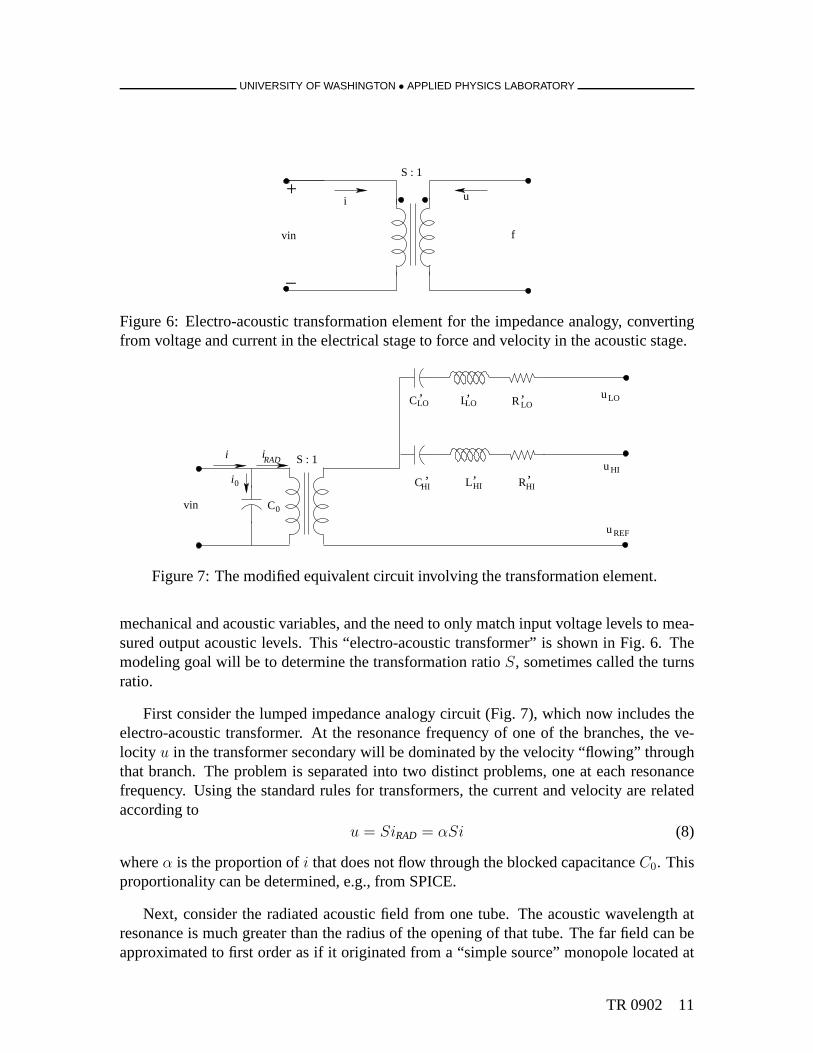
Figure 6: Electro-acoustic transformation element for theimpedance analogy, convertingfrom voltage and current in the electrical stage to force andvelocity in the acoustic stage.
LOu
uREF
uHI
C0
i0
iRAD
LOC ’ LLO ’ LOR ’
CHI ’ LHI ’ RHI ’
S : 1
vin
i
Figure 7: The modified equivalent circuit involving the transformation element.
mechanical and acoustic variables, and the need to only match input voltage levels to mea-sured output acoustic levels. This “electro-acoustic transformer” is shown in Fig. 6. Themodeling goal will be to determine the transformation ratioS, sometimes called the turnsratio.
First consider the lumped impedance analogy circuit (Fig. 7), which now includes theelectro-acoustic transformer. At the resonance frequencyof one of the branches, the ve-locity u in the transformer secondary will be dominated by the velocity “flowing” throughthat branch. The problem is separated into two distinct problems, one at each resonancefrequency. Using the standard rules for transformers, the current and velocity are relatedaccording to
u = SiRAD = αSi (8)
whereα is the proportion ofi that does not flow through the blocked capacitanceC0. Thisproportionality can be determined, e.g., from SPICE.
Next, consider the radiated acoustic field from one tube. Theacoustic wavelength atresonance is much greater than the radius of the opening of that tube. The far field can beapproximated to first order as if it originated from a “simplesource” monopole located at
TR 0902 11
UNIVERSITY OF WASHINGTON • APPLIED PHYSICS LABORATORY
that end of that tube. This is true for both tubes. Thus, let
pM(r) =ΠMeikr
4πr(9)
be the radiated pressure due to a monopole, where|r| = r and i =√−1. The source
strengthΠM is related to the fluid velocity of the monopole via [8]
ΠM = ρckU (10)
wherek = ω/c andU is the volume velocity of the source. For a simple source withradiusa, the volume velocity is4πa2ur, whereur is the radial velocity. A simple sphericalsource is not conceptually accurate for the MP200/TR1446; abetter model might use apiston, with volume velocityU = πa2uz, whereuz is now the velocity of the fluid at theopening of the tube, assumed constant over the opening, normal to the opening. The fluidvelocity ur or uz is provided by the SPICE model: the choice of simple source orpistonvolume velocity is merely a matter of a constant of proportionality, but the choice mustbe consistent with the propagator used to calculate the far field (section 4). To maintainfidelity with the physical model,
ΠM = πa2ρckuz (11)
The two ends of the tube form an ‘acoustic doublet,’ shown schematically in Fig. 8.The total acoustic field at the field point is the superposition of the contributions from bothsources. For measurements in the equatorial plane of the tube (i.e.,r = [xH , 0, 0]), thetwo contributions are in-phase. Thus, ifxH ≫ L (whereL is the length of the tube), themeasured acoustic pressure is
|pH(xH)|2 ≈ 4|pM(xH)|2 (12)
Hence, using Eqs. 9, 11, and 12,
|uz|2 =4x2
H
a2(ρc)2(ka)2|pH(xH)|2 (13)
Equating Eqs. 8 and 13, the far field pressure can be written as
|pH(xH)|2 = B2|i|2 (14)
i.e., the pressure is proportional to the drive current. Theconstant of proportionality, de-noted here byB, consists of several factors:
B2 =a2(ρc)2(ka)2α2S2
4x2H
(15)
12 TR 0902
UNIVERSITY OF WASHINGTON • APPLIED PHYSICS LABORATORY
xH
L/2
L/2 far fieldpressure
z
x
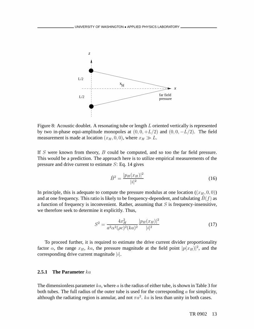
Figure 8: Acoustic doublet. A resonating tube or lengthL oriented vertically is representedby two in-phase equi-amplitude monopoles at(0, 0, +L/2) and (0, 0,−L/2). The fieldmeasurement is made at location(xH , 0, 0), wherexH ≫ L.
If S were known from theory,B could be computed, and so too the far field pressure.This would be a prediction. The approach here is to utilize empirical measurements of thepressure and drive current to estimateS: Eq. 14 gives
B2 =|pH(xH)|2
|i|2 (16)
In principle, this is adequate to compute the pressure modulus at one location ((xH , 0, 0))and at one frequency. This ratio is likely to be frequency-dependent, and tabulatingB(f) asa function of frequency is inconvenient. Rather, assuming thatS is frequency-insensitive,we therefore seek to determine it explicitly. Thus,
S2 =4x2
H
a2α2(ρc)2(ka)2
|pH(xH)|2|i|2 (17)
To proceed further, it is required to estimate the drive current divider proportionalityfactor α, the rangexH , ka, the pressure magnitude at the field point|p(xH)|2, and thecorresponding drive current magnitude|i|.
2.5.1 The Parameterka
The dimensionless parameterka, wherea is the radius of either tube, is shown in Table 3 forboth tubes. The full radius of the outer tube is used for the correspondinga for simplicity,although the radiating region is annular, and notπa2. ka is less than unity in both cases.
TR 0902 13

UNIVERSITY OF WASHINGTON • APPLIED PHYSICS LABORATORY
tube diameter resonancelength [m] [Hz] kalong 0.26 212 0.31short 0.39 320 0.59
Table 3: Values ofka for both tubes.
file peak bin delay [ms] range [m]mptest04.dat 172 21.5 30.7mptest05.dat 173 21.6 30.9mptest06.dat 172 21.5 30.7
Table 4: Slant ranges from transducer to monitor hydrophone, 2006 Lake Washington test.Based on cross-correlation peak. Peak time converted to range using a typical freshwatersound speed of 1430 m/s.
2.5.2 Current Divider Factor
Using the simple circuit (Fig. 2), the proportionality factor α = |iRAD|/|i| can be com-puted using SPICE. For the resonance frequencies 212 and 320Hz, α is 0.98 and 0.54,respectively.
2.5.3 Field Point Range
The m-sequence used to interrogate the transducer is a useful ranging signal. By simplycross-correlating the drive voltage signal against the monitor hydrophone signal, the directpath arrival can be observed as the first prominent peak. For asample rate of 8000 Hz, thesample period was 0.125 ms. Three transmissions from the 2006 Lake Washington exercisewere found to have acceptable drive current and monitor channel data. Table 4 shows theranges estimated for these three transmissions.
2.5.4 Field Pressure
The monitor channel data autospectra were estimated for each corresponding file using theMatlab command
[G,f] = pwelch(x,kaiser(8192),0,8192,8000,’onesided’);
14 TR 0902
UNIVERSITY OF WASHINGTON • APPLIED PHYSICS LABORATORY
0 50 100 150 200 250 300 350 400 450 500−30
−20
−10
0
10
frequency [Hz]
leve
l [dB
re
1 qu
anta
2 /Hz]
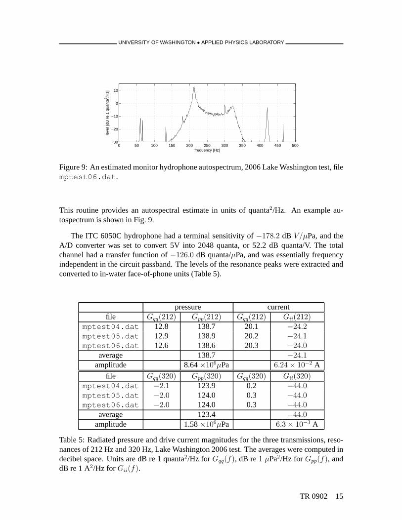
Figure 9: An estimated monitor hydrophone autospectrum, 2006 Lake Washington test, filemptest06.dat.
This routine provides an autospectral estimate in units of quanta2/Hz. An example au-tospectrum is shown in Fig. 9.
The ITC 6050C hydrophone had a terminal sensitivity of−178.2 dB V/µPa, and theA/D converter was set to convert 5V into 2048 quanta, or 52.2 dB quanta/V. The totalchannel had a transfer function of−126.0 dB quanta/µPa, and was essentially frequencyindependent in the circuit passband. The levels of the resonance peaks were extracted andconverted to in-water face-of-phone units (Table 5).
pressure currentfile Gqq(212) Gpp(212) Gqq(212) Gii(212)
mptest04.dat 12.8 138.7 20.1 −24.2mptest05.dat 12.9 138.9 20.2 −24.1mptest06.dat 12.6 138.6 20.3 −24.0
average 138.7 −24.1amplitude 8.64×10⁶µPa 6.24 × 10⁻² A
file Gqq(320) Gpp(320) Gqq(320) Gii(320)mptest04.dat −2.1 123.9 0.2 −44.0mptest05.dat −2.0 124.0 0.3 −44.0mptest06.dat −2.0 124.0 0.3 −44.0
average 123.4 −44.0amplitude 1.58×10⁶µPa 6.3 × 10⁻³ A
Table 5: Radiated pressure and drive current magnitudes forthe three transmissions, reso-nances of 212 Hz and 320 Hz, Lake Washington 2006 test. The averages were computed indecibel space. Units are dB re 1 quanta2/Hz for Gqq(f), dB re 1µPa2/Hz for Gpp(f), anddB re 1 A2/Hz for Gii(f).
TR 0902 15
UNIVERSITY OF WASHINGTON • APPLIED PHYSICS LABORATORY
0 50 100 150 200 250 300 350 400 450 500−20
−10
0
10
20
frequency [Hz]
leve
l [dB
re
1 qu
anta
2 /Hz]
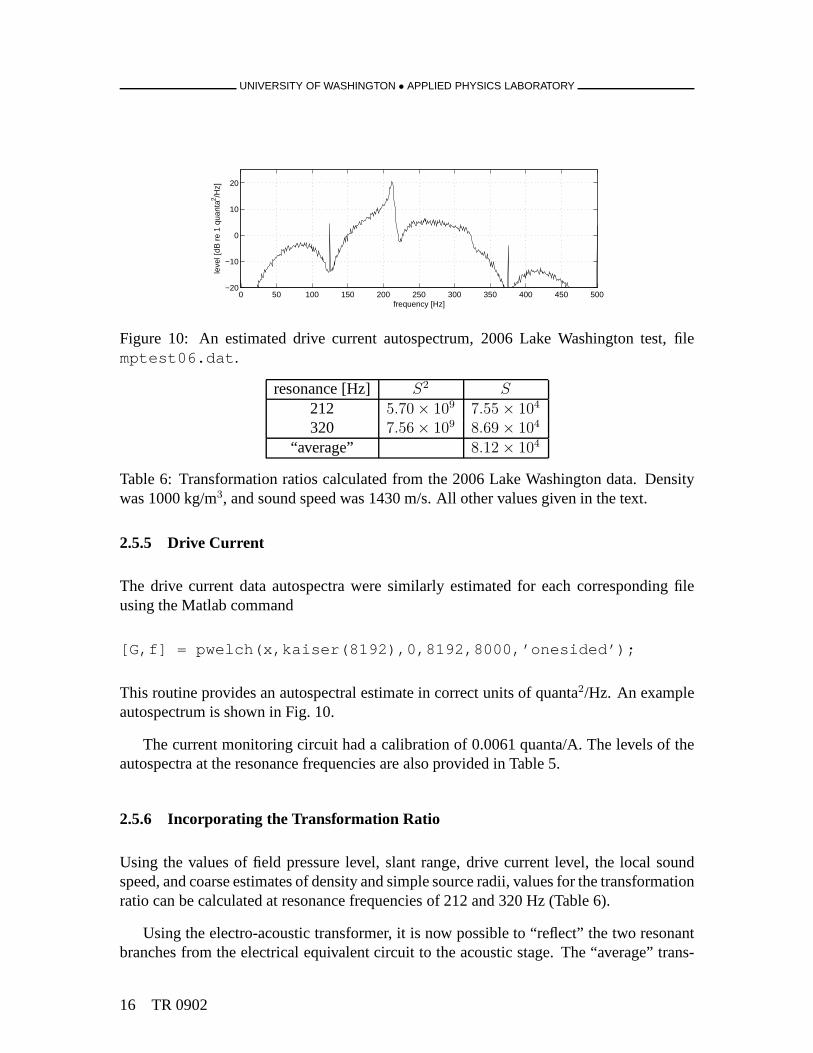
Figure 10: An estimated drive current autospectrum, 2006 Lake Washington test, filemptest06.dat.
resonance [Hz] S2 S212 5.70 × 10⁹ 7.55 × 10⁴
320 7.56 × 10⁹ 8.69 × 10⁴
“average” 8.12 × 10⁴
Table 6: Transformation ratios calculated from the 2006 Lake Washington data. Densitywas 1000 kg/m3, and sound speed was 1430 m/s. All other values given in the text.
2.5.5 Drive Current
The drive current data autospectra were similarly estimated for each corresponding fileusing the Matlab command
[G,f] = pwelch(x,kaiser(8192),0,8192,8000,’onesided’);
This routine provides an autospectral estimate in correct units of quanta2/Hz. An exampleautospectrum is shown in Fig. 10.
The current monitoring circuit had a calibration of 0.0061 quanta/A. The levels of theautospectra at the resonance frequencies are also providedin Table 5.
2.5.6 Incorporating the Transformation Ratio
Using the values of field pressure level, slant range, drive current level, the local soundspeed, and coarse estimates of density and simple source radii, values for the transformationratio can be calculated at resonance frequencies of 212 and 320 Hz (Table 6).
Using the electro-acoustic transformer, it is now possibleto “reflect” the two resonantbranches from the electrical equivalent circuit to the acoustic stage. The “average” trans-
16 TR 0902
UNIVERSITY OF WASHINGTON • APPLIED PHYSICS LABORATORY
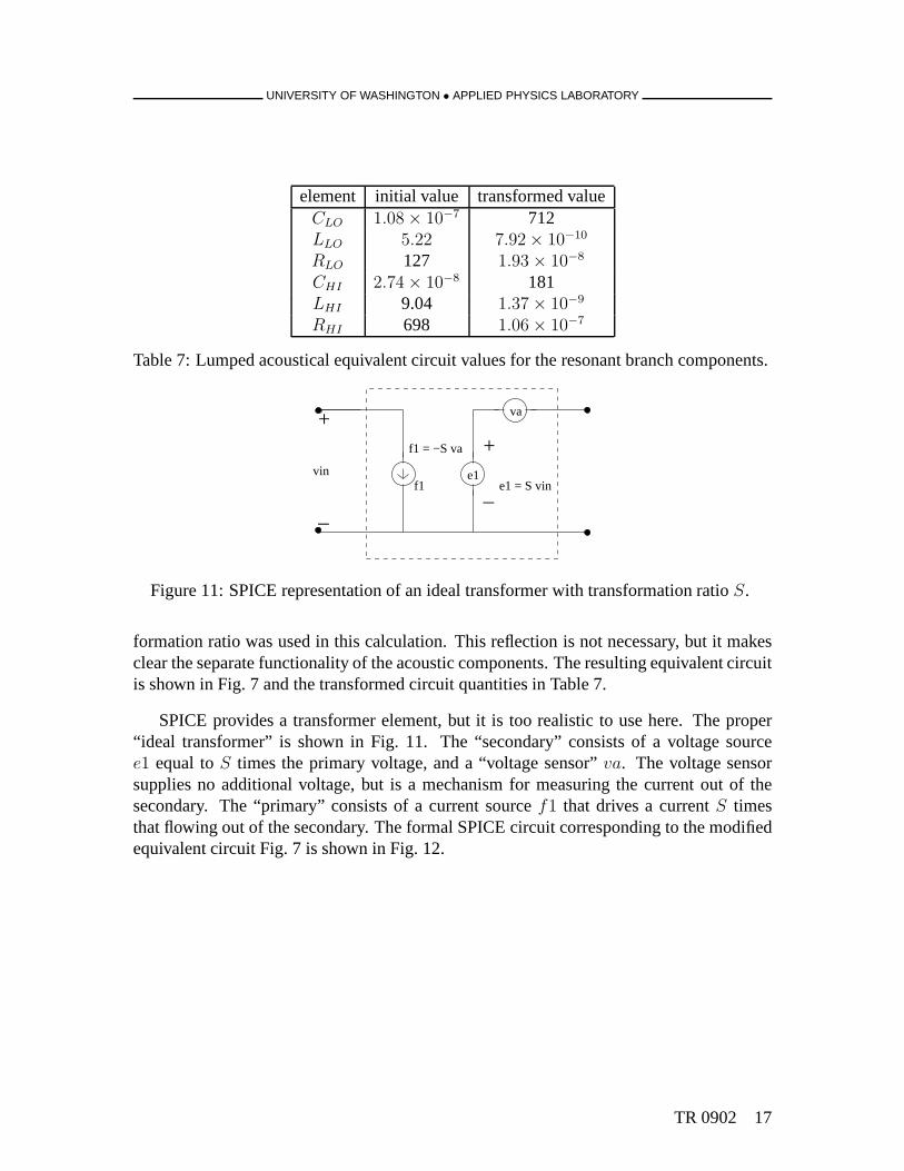
element initial value transformed valueCLO 1.08 × 10⁻⁷ 712LLO 5.22 7.92 × 10⁻¹⁰
RLO 127 1.93 × 10⁻⁸
CHI 2.74 × 10⁻⁸ 181LHI 9.04 1.37 × 10⁻⁹
RHI 698 1.06 × 10⁻⁷
Table 7: Lumped acoustical equivalent circuit values for the resonant branch components.
+
_e1
+
_
va
vin
f1 = −S va
e1 = S vinf1
Figure 11: SPICE representation of an ideal transformer with transformation ratioS.
formation ratio was used in this calculation. This reflection is not necessary, but it makesclear the separate functionality of the acoustic components. The resulting equivalent circuitis shown in Fig. 7 and the transformed circuit quantities in Table 7.
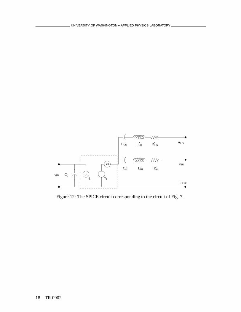
SPICE provides a transformer element, but it is too realistic to use here. The proper“ideal transformer” is shown in Fig. 11. The “secondary” consists of a voltage sourcee1 equal toS times the primary voltage, and a “voltage sensor”va. The voltage sensorsupplies no additional voltage, but is a mechanism for measuring the current out of thesecondary. The “primary” consists of a current sourcef1 that drives a currentS timesthat flowing out of the secondary. The formal SPICE circuit corresponding to the modifiedequivalent circuit Fig. 7 is shown in Fig. 12.
TR 0902 17
UNIVERSITY OF WASHINGTON • APPLIED PHYSICS LABORATORY
C0
LOu
uREF
uHI
f 1e1
CLO ’ L ’ LO LOR ’
RHI ’ LHI ’ CHI ’
vin
va
Figure 12: The SPICE circuit corresponding to the circuit ofFig. 7.
18 TR 0902

UNIVERSITY OF WASHINGTON • APPLIED PHYSICS LABORATORY
3 Tuning
It is advantageous to add a tuner/transformer to a high-power piezoceramic transducer fortwo reasons:
1. The inductance of the tuner/transformer can be used to match the capacitance of thepiezoceramic itself, resulting in a better power factor at the power amplifier, whichresults in more efficient transfer of power to the transducer;
2. The voltage on the suspension cable can be kept within rated levels by utilizing atuner/transformer at the underwater package that includesa step-up ratio.
An autotransformer is generally used in this application, because electrical isolation isnot required, and the autotransformer does not require as massive a core as a conventionaltransformer.
3.1 Single Resonance Theory
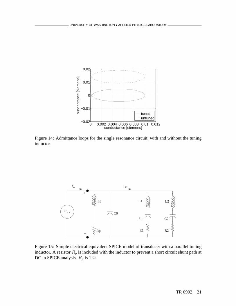
Consider an example circuit (Fig. 13). At the resonance frequency, the untuned circuit hasa power factor of 0.55; the admittance loop is shown in Fig. 14. An inductance value of50 mH brings the power factor to 0.996: the resulting admittance loop is also shown inFig. 14.
Using the equation
P (f) =1
2V (f)∗I(f) = W (f) + jQ(f) (18)
for the average complex power, a SPICE calculation at the resonance frequency shows thatthe ratio of real power delivered by the source (W ) to total power|P (f)| goes from 55% to100%, corresponding to the power factor. Delivery of power at this frequency is optimizedby this inductor.
3.2 Multiple Resonance Theory and Wideband Signals
The conventional approach presented in the previous section is defined for a system witha single resonance at a single frequency. It is not obvious, however, how to extend thoseresults to a system with multiple resonances and wideband signals.
TR 0902 19
UNIVERSITY OF WASHINGTON • APPLIED PHYSICS LABORATORY
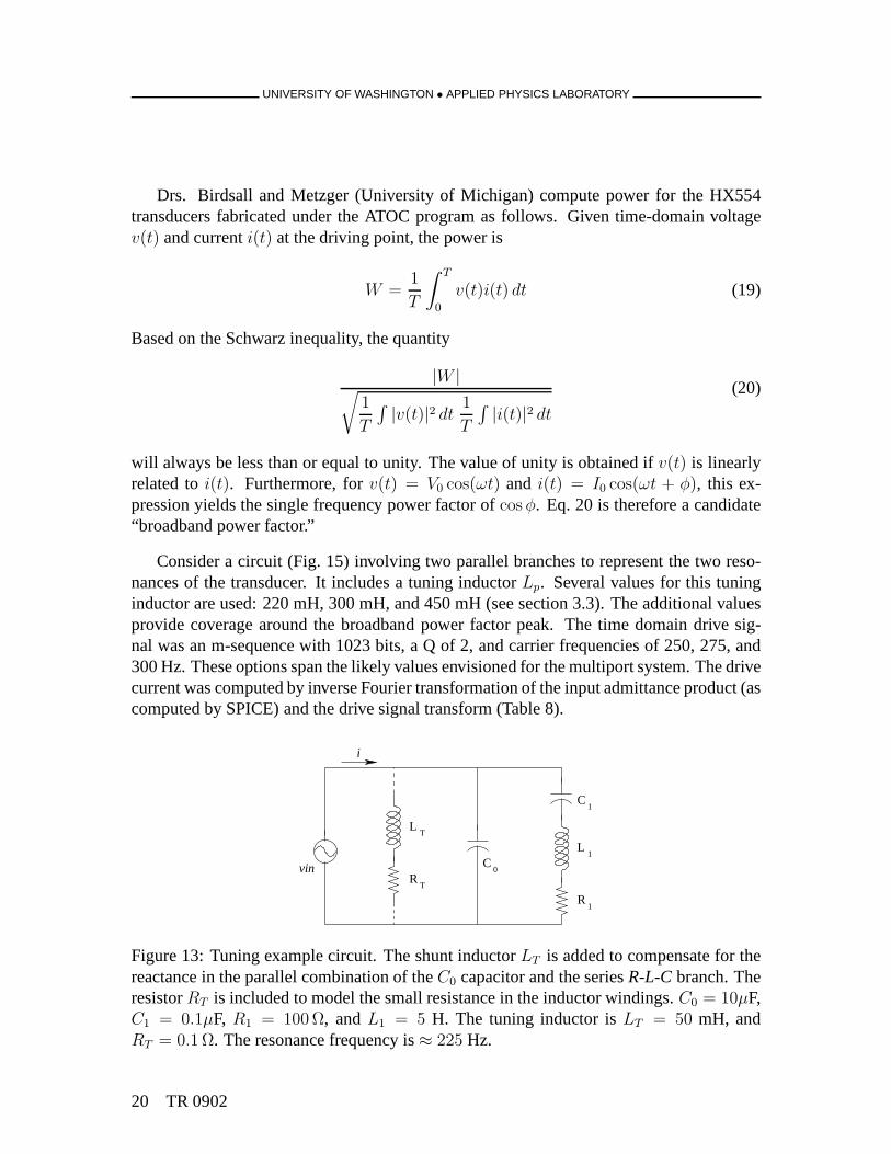
Drs. Birdsall and Metzger (University of Michigan) computepower for the HX554transducers fabricated under the ATOC program as follows. Given time-domain voltagev(t) and currenti(t) at the driving point, the power is
W =1
T
∫ T
0
v(t)i(t) dt (19)
Based on the Schwarz inequality, the quantity
|W |√
1
T
∫
|v(t)|2 dt1
T
∫
|i(t)|2 dt
(20)
will always be less than or equal to unity. The value of unity is obtained ifv(t) is linearlyrelated toi(t). Furthermore, forv(t) = V0 cos(ωt) and i(t) = I0 cos(ωt + φ), this ex-pression yields the single frequency power factor ofcos φ. Eq. 20 is therefore a candidate“broadband power factor.”
Consider a circuit (Fig. 15) involving two parallel branches to represent the two reso-nances of the transducer. It includes a tuning inductorLp. Several values for this tuninginductor are used: 220 mH, 300 mH, and 450 mH (see section 3.3). The additional valuesprovide coverage around the broadband power factor peak. The time domain drive sig-nal was an m-sequence with 1023 bits, a Q of 2, and carrier frequencies of 250, 275, and300 Hz. These options span the likely values envisioned for the multiport system. The drivecurrent was computed by inverse Fourier transformation of the input admittance product (ascomputed by SPICE) and the drive signal transform (Table 8).
LT
RT
C1
L1
R1
0C
i
vin
Figure 13: Tuning example circuit. The shunt inductorLT is added to compensate for thereactance in the parallel combination of theC0 capacitor and the seriesR-L-Cbranch. TheresistorRT is included to model the small resistance in the inductor windings.C0 = 10µF,C1 = 0.1µF, R1 = 100 Ω, andL1 = 5 H. The tuning inductor isLT = 50 mH, andRT = 0.1 Ω. The resonance frequency is≈ 225 Hz.
20 TR 0902
UNIVERSITY OF WASHINGTON • APPLIED PHYSICS LABORATORY
0 0.002 0.004 0.006 0.008 0.01 0.012−0.02
−0.01
0
0.01
0.02
conductance [siemens]
susc
epta
nce
[sie
men
s]
tuneduntuned
Figure 14: Admittance loops for the single resonance circuit, with and without the tuninginductor.
iin 12i
L1 L2
C1 C2
R1 R2
+
_
C0
Rp
Lp
Figure 15: Simple electrical equivalent SPICE model of transducer with a parallel tuninginductor. A resistorRp is included with the inductor to prevent a short circuit shunt path atDC in SPICE analysis.Rp is 1Ω.
TR 0902 21
UNIVERSITY OF WASHINGTON • APPLIED PHYSICS LABORATORY
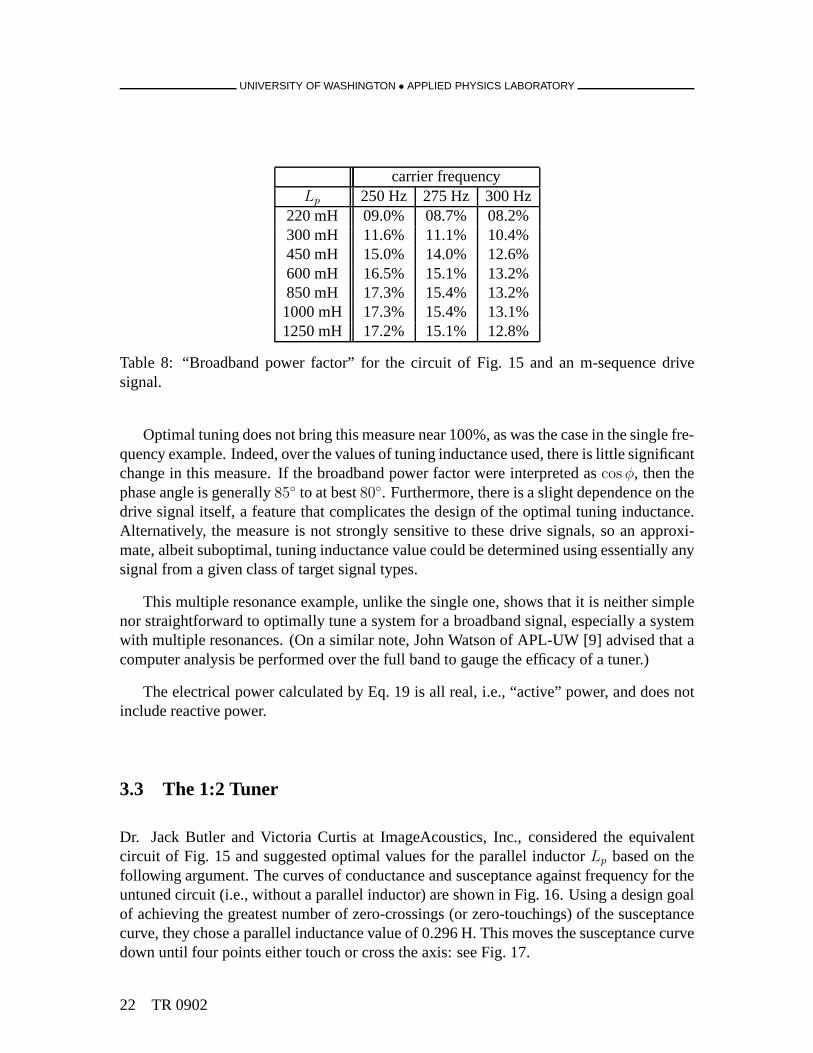
carrier frequencyLp 250 Hz 275 Hz 300 Hz
220 mH 09.0% 08.7% 08.2%300 mH 11.6% 11.1% 10.4%450 mH 15.0% 14.0% 12.6%600 mH 16.5% 15.1% 13.2%850 mH 17.3% 15.4% 13.2%1000 mH 17.3% 15.4% 13.1%1250 mH 17.2% 15.1% 12.8%
Table 8: “Broadband power factor” for the circuit of Fig. 15 and an m-sequence drivesignal.
Optimal tuning does not bring this measure near 100%, as was the case in the single fre-quency example. Indeed, over the values of tuning inductance used, there is little significantchange in this measure. If the broadband power factor were interpreted ascos φ, then thephase angle is generally85 to at best80. Furthermore, there is a slight dependence on thedrive signal itself, a feature that complicates the design of the optimal tuning inductance.Alternatively, the measure is not strongly sensitive to these drive signals, so an approxi-mate, albeit suboptimal, tuning inductance value could be determined using essentially anysignal from a given class of target signal types.
This multiple resonance example, unlike the single one, shows that it is neither simplenor straightforward to optimally tune a system for a broadband signal, especially a systemwith multiple resonances. (On a similar note, John Watson ofAPL-UW [9] advised that acomputer analysis be performed over the full band to gauge the efficacy of a tuner.)
The electrical power calculated by Eq. 19 is all real, i.e., “active” power, and does notinclude reactive power.
3.3 The 1:2 Tuner
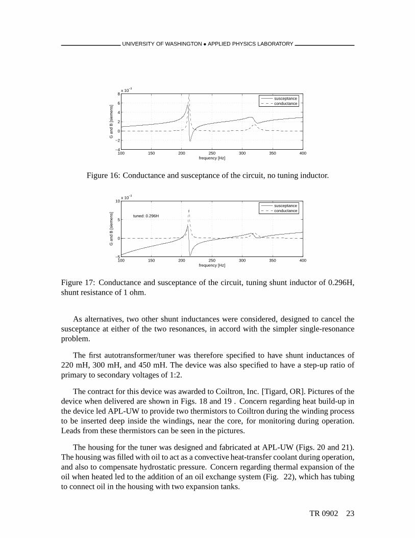
Dr. Jack Butler and Victoria Curtis at ImageAcoustics, Inc., considered the equivalentcircuit of Fig. 15 and suggested optimal values for the parallel inductorLp based on thefollowing argument. The curves of conductance and susceptance against frequency for theuntuned circuit (i.e., without a parallel inductor) are shown in Fig. 16. Using a design goalof achieving the greatest number of zero-crossings (or zero-touchings) of the susceptancecurve, they chose a parallel inductance value of 0.296 H. This moves the susceptance curvedown until four points either touch or cross the axis: see Fig. 17.
22 TR 0902
UNIVERSITY OF WASHINGTON • APPLIED PHYSICS LABORATORY
100 150 200 250 300 350 400−4
−2
0
2
4
6
8x 10
−3
frequency [Hz]
G a
nd B
[sie
men
s]
susceptanceconductance
Figure 16: Conductance and susceptance of the circuit, no tuning inductor.
100 150 200 250 300 350 400−5
0
5
10x 10
−3
frequency [Hz]
G a
nd B
[sie
men
s] tuned: 0.296H
susceptanceconductance
Figure 17: Conductance and susceptance of the circuit, tuning shunt inductor of 0.296H,shunt resistance of 1 ohm.
As alternatives, two other shunt inductances were considered, designed to cancel thesusceptance at either of the two resonances, in accord with the simpler single-resonanceproblem.
The first autotransformer/tuner was therefore specified to have shunt inductances of220 mH, 300 mH, and 450 mH. The device was also specified to havea step-up ratio ofprimary to secondary voltages of 1:2.
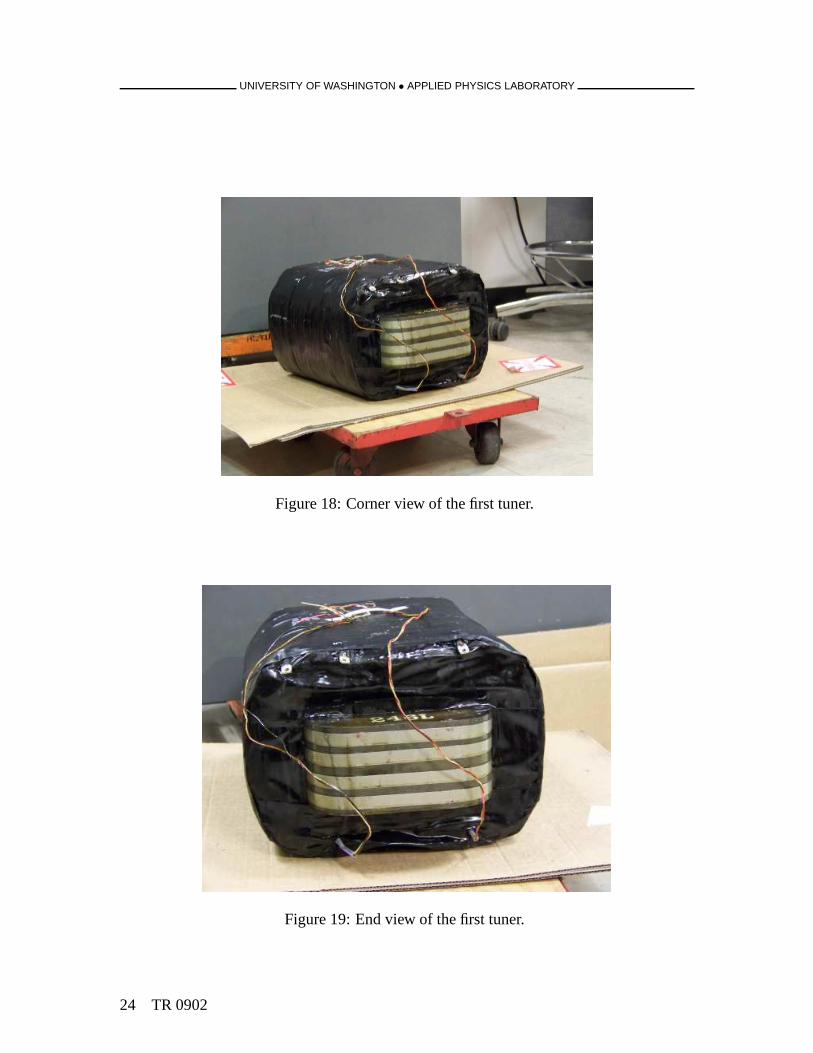
The contract for this device was awarded to Coiltron, Inc. [Tigard, OR]. Pictures of thedevice when delivered are shown in Figs. 18 and 19 . Concern regarding heat build-up inthe device led APL-UW to provide two thermistors to Coiltronduring the winding processto be inserted deep inside the windings, near the core, for monitoring during operation.Leads from these thermistors can be seen in the pictures.
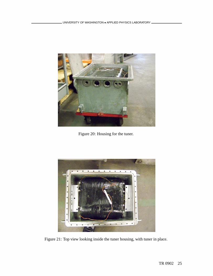
The housing for the tuner was designed and fabricated at APL-UW (Figs. 20 and 21).The housing was filled with oil to act as a convective heat-transfer coolant during operation,and also to compensate hydrostatic pressure. Concern regarding thermal expansion of theoil when heated led to the addition of an oil exchange system (Fig. 22), which has tubingto connect oil in the housing with two expansion tanks.
TR 0902 23
UNIVERSITY OF WASHINGTON • APPLIED PHYSICS LABORATORY
Figure 18: Corner view of the first tuner.
Figure 19: End view of the first tuner.
24 TR 0902
UNIVERSITY OF WASHINGTON • APPLIED PHYSICS LABORATORY
Figure 20: Housing for the tuner.
Figure 21: Top view looking inside the tuner housing, with tuner in place.
TR 0902 25
UNIVERSITY OF WASHINGTON • APPLIED PHYSICS LABORATORY
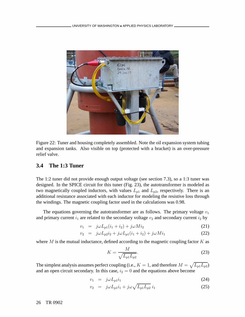
Figure 22: Tuner and housing completely assembled. Note theoil expansion system tubingand expansion tanks. Also visible on top (protected with a bracket) is an over-pressurerelief valve.
3.4 The 1:3 Tuner
The 1:2 tuner did not provide enough output voltage (see section 7.3), so a 1:3 tuner wasdesigned. In the SPICE circuit for this tuner (Fig. 23), the autotransformer is modeled astwo magnetically coupled inductors, with valuesLp1 andLp2, respectively. There is anadditional resistance associated with each inductor for modeling the resistive loss throughthe windings. The magnetic coupling factor used in the calculations was 0.98.
The equations governing the autotransformer are as follows. The primary voltagev1
and primary currenti1 are related to the secondary voltagev2 and secondary currenti2 by
v1 = jωLp1(i1 + i2) + jωMi2 (21)
v2 = jωLp2i2 + jωLp1(i1 + i2) + jωMi1 (22)
whereM is the mutual inductance, defined according to the magnetic coupling factorK as
K =M
√
Lp1Lp2
. (23)
The simplest analysis assumes perfect coupling (i.e.,K = 1, and thereforeM =√
Lp1Lp2)and an open circuit secondary. In this case,i2 = 0 and the equations above become
v1 = jωLp1i1 (24)
v2 = jωLp1i1 + jω√
Lp1Lp2 i1 (25)
26 TR 0902
UNIVERSITY OF WASHINGTON • APPLIED PHYSICS LABORATORY
2i2v
1vL1 L2
C1 C2
R1 R2
C0i1
Lp2
Rp2
Lp1
Rp1
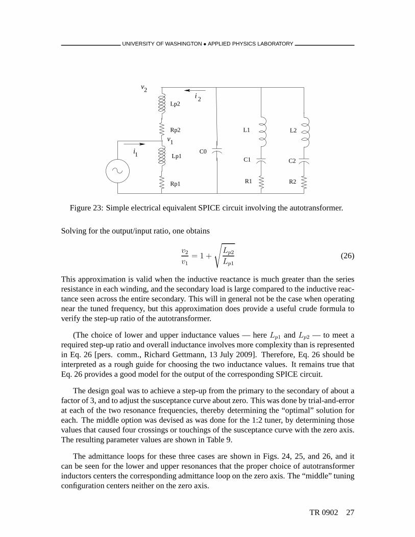
Figure 23: Simple electrical equivalent SPICE circuit involving the autotransformer.
Solving for the output/input ratio, one obtains
v2
v1
= 1 +
√
Lp2
Lp1
(26)
This approximation is valid when the inductive reactance ismuch greater than the seriesresistance in each winding, and the secondary load is large compared to the inductive reac-tance seen across the entire secondary. This will in generalnot be the case when operatingnear the tuned frequency, but this approximation does provide a useful crude formula toverify the step-up ratio of the autotransformer.
(The choice of lower and upper inductance values — hereLp1 andLp2 — to meet arequired step-up ratio and overall inductance involves more complexity than is representedin Eq. 26 [pers. comm., Richard Gettmann, 13 July 2009]. Therefore, Eq. 26 should beinterpreted as a rough guide for choosing the two inductancevalues. It remains true thatEq. 26 provides a good model for the output of the corresponding SPICE circuit.
The design goal was to achieve a step-up from the primary to the secondary of about afactor of 3, and to adjust the susceptance curve about zero. This was done by trial-and-errorat each of the two resonance frequencies, thereby determining the “optimal” solution foreach. The middle option was devised as was done for the 1:2 tuner, by determining thosevalues that caused four crossings or touchings of the susceptance curve with the zero axis.The resulting parameter values are shown in Table 9.
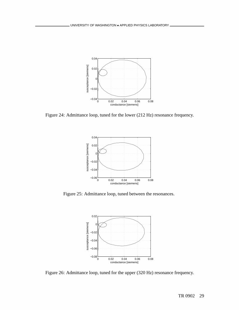
The admittance loops for these three cases are shown in Figs.24, 25, and 26, and itcan be seen for the lower and upper resonances that the properchoice of autotransformerinductors centers the corresponding admittance loop on thezero axis. The “middle” tuningconfiguration centers neither on the zero axis.
TR 0902 27
UNIVERSITY OF WASHINGTON • APPLIED PHYSICS LABORATORY
Lp1 Lp2
low freq 50 mH 210 mHmid freq 33 mH 130 mHhi freq 22 mH 90 mH
Table 9: Upper and lower inductor values for tuning the circuit, at three different frequen-cies, 1:3 step-up.
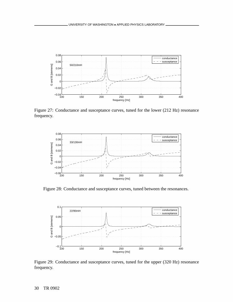
The corresponding conductance and susceptance curves for these three cases are shownin Figs. 27, 28, and 29. The “middle” tuning can be verified here as that configuration thatcauses four crossings or touchings.
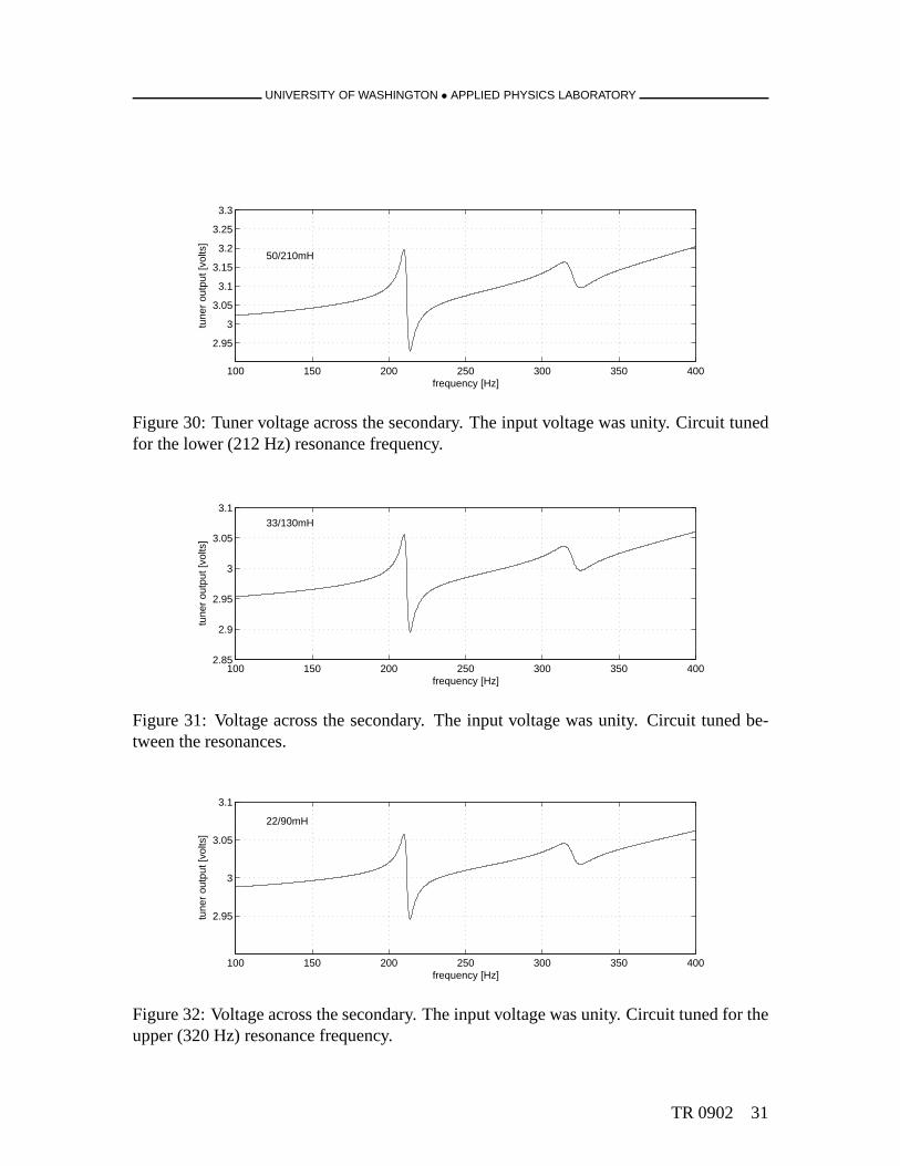
As an additional verification, the tuner output (autotransformer secondary) is plottedversus frequency for all three tuning configurations in Figs. 30, 31, and 32. The inputvoltage in all cases was uniform across all frequencies at1+0j. These figures indicate thatthe autotransformer secondary output is load dependent forthese load magnitudes, but thatthe output–input ratio is close to the design value of 3 for all frequencies considered.
28 TR 0902
UNIVERSITY OF WASHINGTON • APPLIED PHYSICS LABORATORY
0 0.02 0.04 0.06 0.08−0.04
−0.02
0
0.02
0.04
conductance [siemens]
susc
epta
nce
[sie
men
s]
Figure 24: Admittance loop, tuned for the lower (212 Hz) resonance frequency.
0 0.02 0.04 0.06 0.08−0.06
−0.04
−0.02
0
0.02
0.04
conductance [siemens]
susc
epta
nce
[sie
men
s]
Figure 25: Admittance loop, tuned between the resonances.
0 0.02 0.04 0.06 0.08−0.08
−0.06
−0.04
−0.02
0
0.02
conductance [siemens]
susc
epta
nce
[sie
men
s]
Figure 26: Admittance loop, tuned for the upper (320 Hz) resonance frequency.
TR 0902 29
UNIVERSITY OF WASHINGTON • APPLIED PHYSICS LABORATORY
100 150 200 250 300 350 400−0.04
−0.02
0
0.02
0.04
0.06
0.08
frequency [Hz]
G a
nd B
[sie
men
s] 50/210mH
conductancesusceptance
Figure 27: Conductance and susceptance curves, tuned for the lower (212 Hz) resonancefrequency.
100 150 200 250 300 350 400−0.06
−0.04
−0.02
0
0.02
0.04
0.06
0.08
frequency [Hz]
G a
nd B
[sie
men
s] 33/130mH
conductancesusceptance
Figure 28: Conductance and susceptance curves, tuned between the resonances.
100 150 200 250 300 350 400−0.1
−0.05
0
0.05
0.1
frequency [Hz]
G a
nd B
[sie
men
s]
22/90mH conductancesusceptance
Figure 29: Conductance and susceptance curves, tuned for the upper (320 Hz) resonancefrequency.
30 TR 0902
UNIVERSITY OF WASHINGTON • APPLIED PHYSICS LABORATORY
100 150 200 250 300 350 400
2.95
3
3.05
3.1
3.15
3.2
3.25
3.3
frequency [Hz]
tune
r ou
tput
[vol
ts]
50/210mH
Figure 30: Tuner voltage across the secondary. The input voltage was unity. Circuit tunedfor the lower (212 Hz) resonance frequency.
100 150 200 250 300 350 4002.85
2.9
2.95
3
3.05
3.1
frequency [Hz]
tune
r ou
tput
[vol
ts]
33/130mH
Figure 31: Voltage across the secondary. The input voltage was unity. Circuit tuned be-tween the resonances.
100 150 200 250 300 350 400
2.95
3
3.05
3.1
frequency [Hz]
tune
r ou
tput
[vol
ts]
22/90mH
Figure 32: Voltage across the secondary. The input voltage was unity. Circuit tuned for theupper (320 Hz) resonance frequency.
TR 0902 31

UNIVERSITY OF WASHINGTON • APPLIED PHYSICS LABORATORY
4 The Multiport System
An essential system block diagram of the APL-UW system (Fig.33) shows the underwatersubsystem components:
• the MP200/TR1446 with the tuner
• a monitor hydrophone
• a custom telemetry bottle with a fibre-optic interface
• a depth sensor
• a SeaBattery
poweramplifier
winch
interfacefibre
computertracking
GPS
telemetrybottle
interrogatortracking
monitorhydrophone
interfaceunit
LPF
shipboard componentssignal computer
GPS
underwatersubsystem
SeaBattery
transducer
tuner
Figure 33: Block diagram of essential components for the complete multiport system.
32 TR 0902
UNIVERSITY OF WASHINGTON • APPLIED PHYSICS LABORATORY
The ship-side equipment consists of a signal delivery rack,which includes a 80686PC running Fedora Core 8 Linux, a Spectrum Instruments TM-4 GPS receiver, a custominterface unit, and a Krohn–Hite filter; a power amplifier; a custom winch; and a trackingsystem. The original power amplifier was a Ling. An L50 amplifier was procured fromInstruments, Inc., for the Philippine Sea experiments.
The underwater package is suspended from an “electro-opto-mechanical” cable. Teleme-try information utilizes the fibre, and transducer power utilizes the copper conductor. Inpractice, the underwater package is deployed and recoveredby the custom winch.
SeaBattery& telemetry
tuner
suspensioncable
Figure 34: Schematic of the initialmechanical configuration.
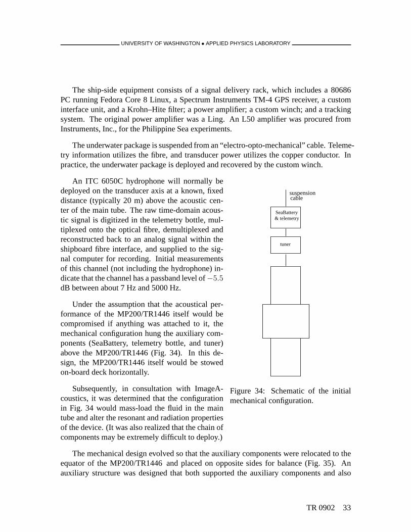
An ITC 6050C hydrophone will normally bedeployed on the transducer axis at a known, fixeddistance (typically 20 m) above the acoustic cen-ter of the main tube. The raw time-domain acous-tic signal is digitized in the telemetry bottle, mul-tiplexed onto the optical fibre, demultiplexed andreconstructed back to an analog signal within theshipboard fibre interface, and supplied to the sig-nal computer for recording. Initial measurementsof this channel (not including the hydrophone) in-dicate that the channel has a passband level of−5.5dB between about 7 Hz and 5000 Hz.
Under the assumption that the acoustical per-formance of the MP200/TR1446 itself would becompromised if anything was attached to it, themechanical configuration hung the auxiliary com-ponents (SeaBattery, telemetry bottle, and tuner)above the MP200/TR1446 (Fig. 34). In this de-sign, the MP200/TR1446 itself would be stowedon-board deck horizontally.
Subsequently, in consultation with ImageA-coustics, it was determined that the configurationin Fig. 34 would mass-load the fluid in the maintube and alter the resonant and radiation propertiesof the device. (It was also realized that the chain ofcomponents may be extremely difficult to deploy.)
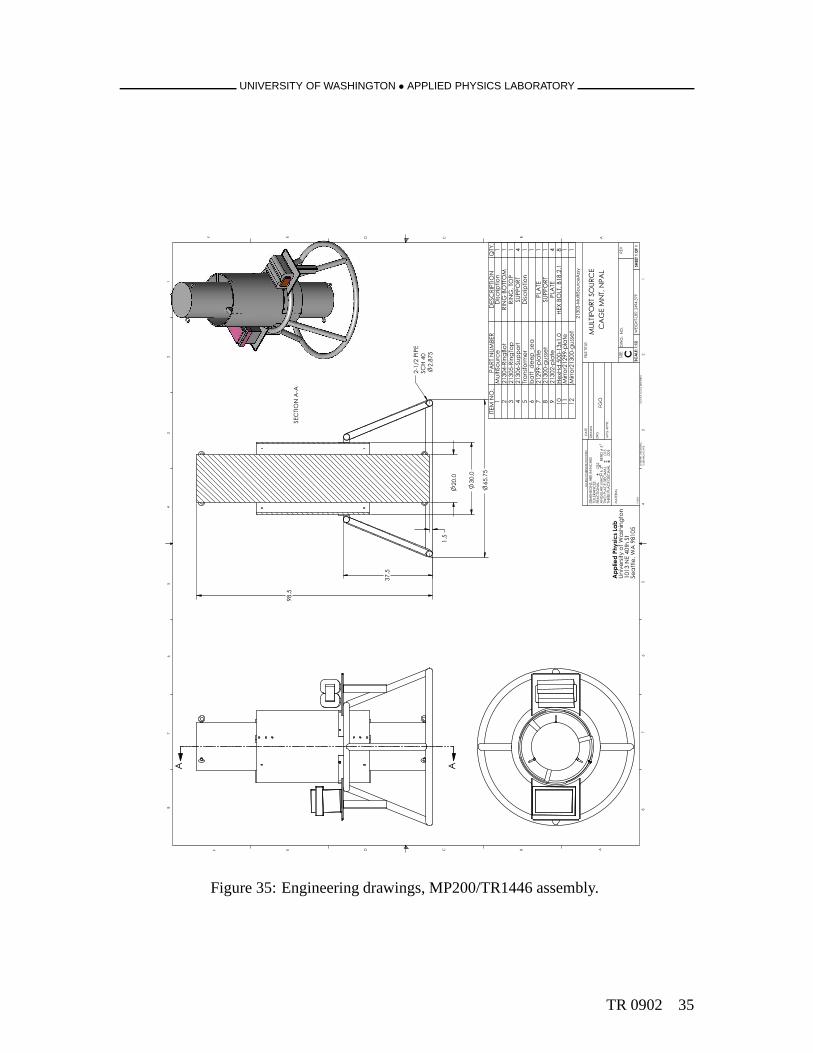
The mechanical design evolved so that the auxiliary components were relocated to theequator of the MP200/TR1446 and placed on opposite sides forbalance (Fig. 35). Anauxiliary structure was designed that both supported the auxiliary components and also
TR 0902 33
UNIVERSITY OF WASHINGTON • APPLIED PHYSICS LABORATORY
supported the MP200/TR1446 in an upright position while on deck. Although massive, theSeaBattery and the tuner were small relative to a wavelength, and therefore their modifi-cation to the radiated acoustical field should be small as long as they are away from thetube openings. The support structure itself was fabricatedfrom free-flooded steel tubing,which also should have a negligible acoustical cross-section. No modeling has been doneto quantify the effect of these auxiliary components on the radiated acoustical field.
With the design complete, it was realized that the entire system would be too tall to belifted from the deck using a chain bridle attached to the bolteyes fixed into the top of themain tube. A tentative plan was devised to lift from a hard point welded onto the main tubeexactly at the top of the secondary tube, i.e., lifting the entire system from one “shoulder.”This plan introduced a further problem: the system would hang at an angle significantly offvertical. Further calculations showed, however, that a lifting point located at the center ofa cross-bar bolted into the mouth of the main tube several centimeters down from the topwould provide enough clearance. The cross-bar width was much less than a wavelengthand overall cross-sectional area much less than the area of the main tube opening, so thisbar is not expected to modify the resonant or radiation patterns significantly. In the finalanalysis, the system was calculated to hang about2.6 off vertical.
34 TR 0902
UNIVERSITY OF WASHINGTON • APPLIED PHYSICS LABORATORY
57.
56
baL s
cisy
hP
deil
pp
An
otg
nihs
aW f
o ytisr
evi
nU
tS
ht0
4 E
N 3
10
15
01
89
AW ,
eltta
eS
.YT
QN
OITPI
RC
SE
DR
EB
MU
N TR
AP
.O
N M
ETI1
noit
pircsi
De
cru
oSitl
uM
11
MOTT
OB
GNI
Rt
oB
gni
R-4
03
12
21
POT ,
GNI
Rp
oTg
niR-
50
31
23
4T
RO
PP
US
tro
pp
uS-
60
31
24
1n
oitpir
csiD
re
mrofs
narT
51
aes
_p
ee
d_tt
ab
61
ETAL
Pet
alp-
99
21
27
1T
RO
PP
US
tess
ug-
00
31
28
4ET
ALP
etal
p-2
03
12
98
1.2.
81
B ,TLO
B X
EH
0.1
x3
1-0
05.
dH
xe
H0
11
etal
p-9
92
12r
orriM
11
1t
essu
g -0
03
12r
o rriM
21
A-A
NOIT
CE
S
5.7
3
04
HC
SE
PIP
2/1-
2
57
8.2
5.8
9
5.1
0.0
2
0.0
3
GNI
WA
RD
ELA
CS T
ON
OD
LA
PN ,T
NM
EG
AC
D C B
ABCD
12
34
56
78
85
67
43
21
EF
AEF
1 FO
1 TE
EH
S
yssA
ecr
uo
Sitlu
M-3
03
12
EC
RU
OS T
RO
PITLU
M
21:
1 :EL
AC
S9
73.
49
42 :
SBL-T
HGI
EW
VE
R.
ON .
GW
D
CEZIS
:ELTIT
ELIFET
AD
.R
PP
A GF
M
G
NE
NW
AR
D
HSI
N IF
:D
EI FIC
EP
S E
SIW
RE
HTO
SS
ELN
U
:R
EP
GNI
CN
AR
ELOT
LAI
RET
AM
50
0.
CIRT
EM
OE
G TE
RP
RET
NI
SE
HC
NI NI
ER
A S
NOI
SN
EMI
D :
SE
CN
AR
ELOT
LA
NOIT
CA
RF2
30.
HC
AM :
RAL
UG
NA
2
DN
EB
5 L
AMI
CE
D E
CAL
P O
WT5
10.
LA
MIC
ED
EC
ALP
EE
RHT
OGF
A A
Figure 35: Engineering drawings, MP200/TR1446 assembly.
TR 0902 35
UNIVERSITY OF WASHINGTON • APPLIED PHYSICS LABORATORY
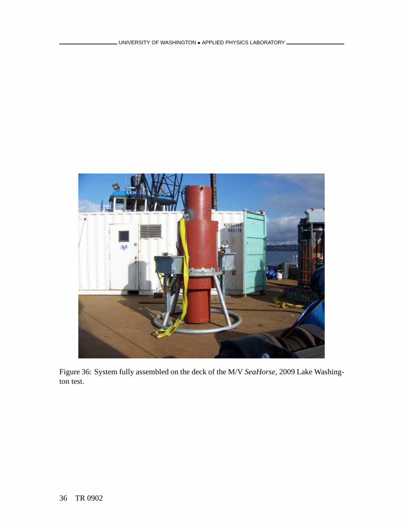
Figure 36: System fully assembled on the deck of the M/VSeaHorse, 2009 Lake Washing-ton test.
36 TR 0902
UNIVERSITY OF WASHINGTON • APPLIED PHYSICS LABORATORY
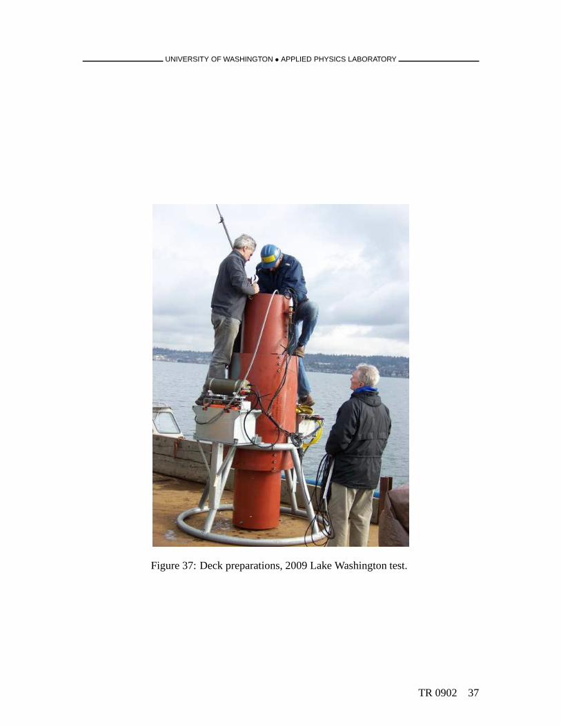
Figure 37: Deck preparations, 2009 Lake Washington test.
TR 0902 37
UNIVERSITY OF WASHINGTON • APPLIED PHYSICS LABORATORY
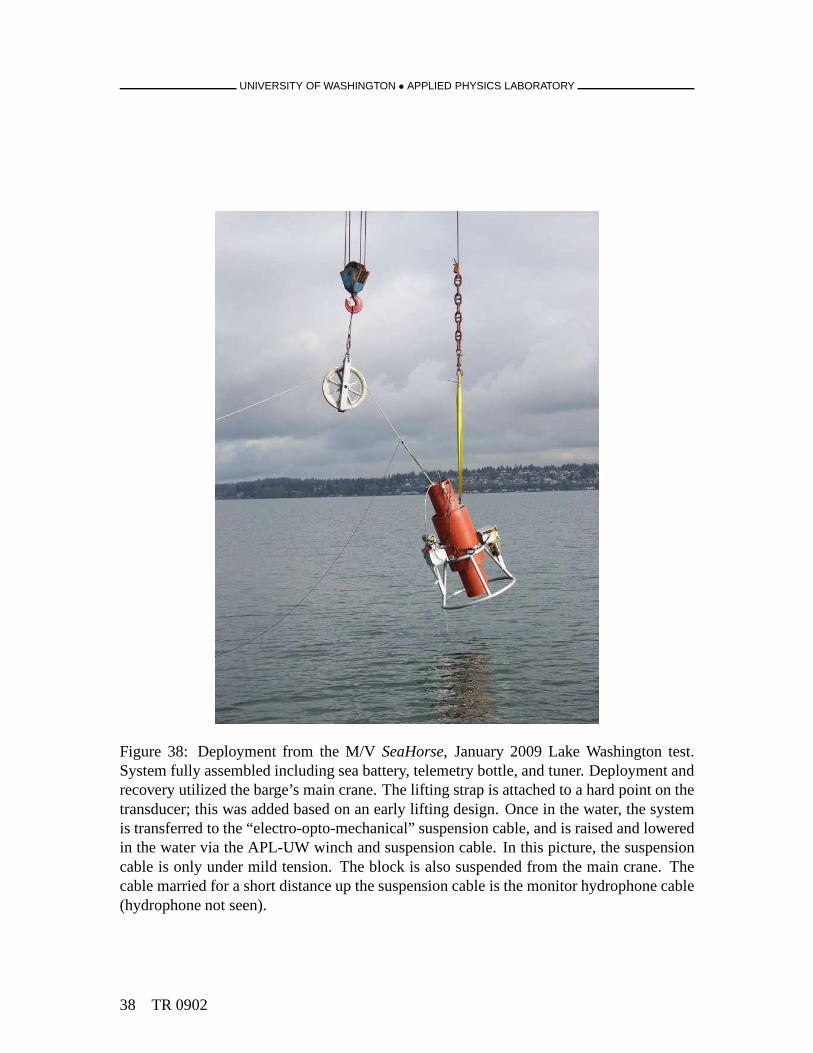
Figure 38: Deployment from the M/VSeaHorse, January 2009 Lake Washington test.System fully assembled including sea battery, telemetry bottle, and tuner. Deployment andrecovery utilized the barge’s main crane. The lifting strapis attached to a hard point on thetransducer; this was added based on an early lifting design.Once in the water, the systemis transferred to the “electro-opto-mechanical” suspension cable, and is raised and loweredin the water via the APL-UW winch and suspension cable. In this picture, the suspensioncable is only under mild tension. The block is also suspendedfrom the main crane. Thecable married for a short distance up the suspension cable isthe monitor hydrophone cable(hydrophone not seen).
38 TR 0902
UNIVERSITY OF WASHINGTON • APPLIED PHYSICS LABORATORY
5 System Model
5.1 Introduction
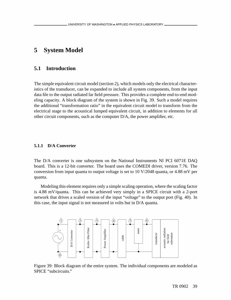
The simple equivalent circuit model (section 2), which models only the electrical character-istics of the transducer, can be expanded to include all system components, from the inputdata file to the output radiated far field pressure. This provides a complete end-to-end mod-eling capacity. A block diagram of the system is shown in Fig.39. Such a model requiresthe additional “transformation ratio” in the equivalent circuit model to transform from theelectrical stage to the acoustical lumped equivalent circuit, in addition to elements for allother circuit components, such as the computer D/A, the power amplifier, etc.
5.1.1 D/A Converter
The D/A converter is one subsystem on the National Instruments NI PCI 6071E DAQboard. This is a 12-bit converter. The board uses the COMEDI driver, version 7.76. Theconversion from input quanta to output voltage is set to 10 V/2048 quanta, or 4.88 mV perquanta.
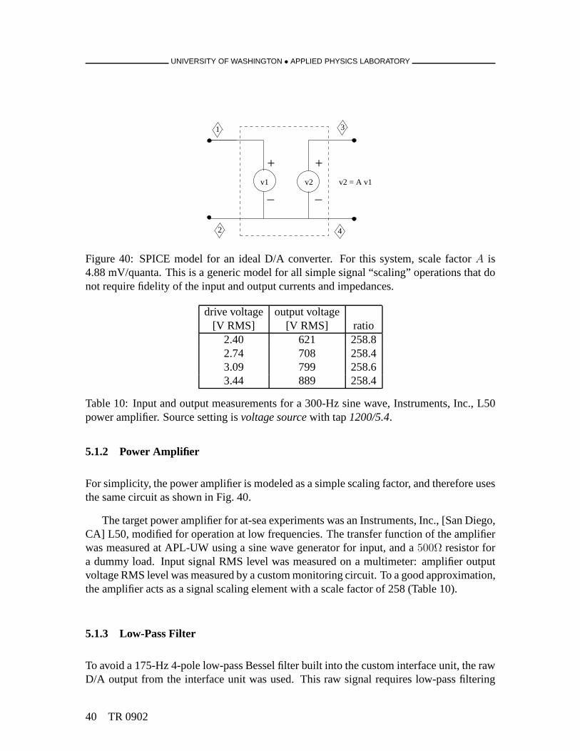
Modeling this element requires only a simple scaling operation, where the scaling factoris 4.88 mV/quanta. This can be achieved very simply in a SPICEcircuit with a 2-portnetwork that drives a scaled version of the input “voltage” to the output port (Fig. 40). Inthis case, the input signal is not measured in volts but in D/Aquanta.
1 3 4 5 6
0
2
tran
sduc
er
cabl
e
Kro
hn−
Hite
Filt
er
D/A
Con
vert
er
Pow
er A
mpl
ifier+
_ far
field
acou
stic
rad
iatio
n
subr
outin
etune
r
Figure 39: Block diagram of the entire system. The individual components are modeled asSPICE “subcircuits.”
TR 0902 39
UNIVERSITY OF WASHINGTON • APPLIED PHYSICS LABORATORY
1
2
3
4
+
_
+
_v2 = A v1v2v1
Figure 40: SPICE model for an ideal D/A converter. For this system, scale factorA is4.88 mV/quanta. This is a generic model for all simple signal“scaling” operations that donot require fidelity of the input and output currents and impedances.
drive voltage output voltage[V RMS] [V RMS] ratio
2.40 621 258.82.74 708 258.43.09 799 258.63.44 889 258.4
Table 10: Input and output measurements for a 300-Hz sine wave, Instruments, Inc., L50power amplifier. Source setting isvoltage sourcewith tap1200/5.4.
5.1.2 Power Amplifier
For simplicity, the power amplifier is modeled as a simple scaling factor, and therefore usesthe same circuit as shown in Fig. 40.
The target power amplifier for at-sea experiments was an Instruments, Inc., [San Diego,CA] L50, modified for operation at low frequencies. The transfer function of the amplifierwas measured at APL-UW using a sine wave generator for input,and a500Ω resistor fora dummy load. Input signal RMS level was measured on a multimeter: amplifier outputvoltage RMS level was measured by a custom monitoring circuit. To a good approximation,the amplifier acts as a signal scaling element with a scale factor of 258 (Table 10).
5.1.3 Low-Pass Filter
To avoid a 175-Hz 4-pole low-pass Bessel filter built into thecustom interface unit, the rawD/A output from the interface unit was used. This raw signal requires low-pass filtering
40 TR 0902
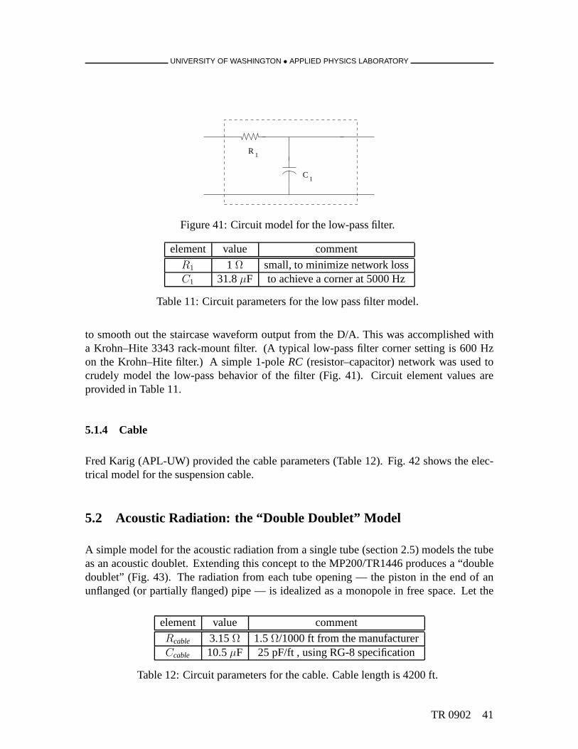
UNIVERSITY OF WASHINGTON • APPLIED PHYSICS LABORATORY
C1
R1
Figure 41: Circuit model for the low-pass filter.
element value comment
R1 1 Ω small, to minimize network lossC1 31.8µF to achieve a corner at 5000 Hz
Table 11: Circuit parameters for the low pass filter model.
to smooth out the staircase waveform output from the D/A. This was accomplished witha Krohn–Hite 3343 rack-mount filter. (A typical low-pass filter corner setting is 600 Hzon the Krohn–Hite filter.) A simple 1-poleRC (resistor–capacitor) network was used tocrudely model the low-pass behavior of the filter (Fig. 41). Circuit element values areprovided in Table 11.
5.1.4 Cable
Fred Karig (APL-UW) provided the cable parameters (Table 12). Fig. 42 shows the elec-trical model for the suspension cable.
5.2 Acoustic Radiation: the “Double Doublet” Model
A simple model for the acoustic radiation from a single tube (section 2.5) models the tubeas an acoustic doublet. Extending this concept to the MP200/TR1446 produces a “doubledoublet” (Fig. 43). The radiation from each tube opening — the piston in the end of anunflanged (or partially flanged) pipe — is idealized as a monopole in free space. Let the
element value comment
Rcable 3.15Ω 1.5Ω/1000 ft from the manufacturerCcable 10.5µF 25 pF/ft , using RG-8 specification
Table 12: Circuit parameters for the cable. Cable length is 4200 ft.
TR 0902 41
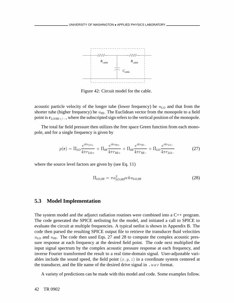
UNIVERSITY OF WASHINGTON • APPLIED PHYSICS LABORATORY
R R
Ccable
cablecable
Figure 42: Circuit model for the cable.
acoustic particle velocity of the longer tube (lower frequency) beuLO and that from theshorter tube (higher frequency) beuHI. The Euclidean vector from the monopole to a fieldpoint isrLO/HI+/−, where the subscripted sign refers to the vertical positionof the monopole.
The total far field pressure then utilizes the free space Green function from each mono-pole, and for a single frequency is given by
p(r) = ΠLOeikrLO+
4πrLO+
+ ΠHIeikrHI+
4πrHI++ ΠHI
eikrHI−
4πrHI−+ ΠLO
eikrLO−
4πrLO−
(27)
where the source level factors are given by (see Eq. 11)
ΠLO,HI = πa2
LO,HIρckuLO,HI (28)
5.3 Model Implementation
The system model and the adjunct radiation routines were combined into a C++ program.The code generated the SPICE netlisting for the model, and initiated a call to SPICE toevaluate the circuit at multiple frequencies. A typical netlist is shown in Appendix B. Thecode then parsed the resulting SPICE output file to retrieve the transducer fluid velocitiesuLO anduHI. The code then used Eqs. 27 and 28 to compute the complex acoustic pres-sure response at each frequency at the desired field point. The code next multiplied theinput signal spectrum by the complex acoustic pressure response at each frequency, andinverse Fourier transformed the result to a real time-domain signal. User-adjustable vari-ables include the sound speed, the field point(x, y, z) in a coordinate system centered atthe transducer, and the file name of the desired drive signal in .wav format.
A variety of predictions can be made with this model and code.Some examples follow.
42 TR 0902
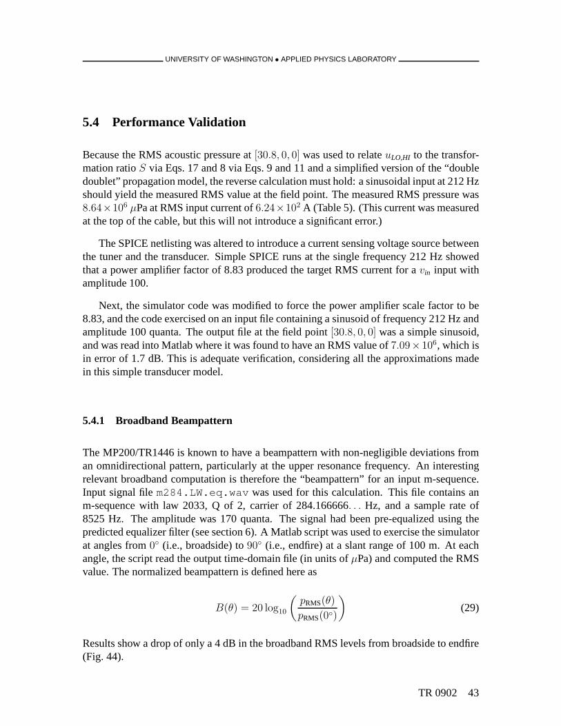
UNIVERSITY OF WASHINGTON • APPLIED PHYSICS LABORATORY
5.4 Performance Validation
Because the RMS acoustic pressure at[30.8, 0, 0] was used to relateuLO,HI to the transfor-mation ratioS via Eqs. 17 and 8 via Eqs. 9 and 11 and a simplified version of the“doubledoublet” propagation model, the reverse calculation must hold: a sinusoidal input at 212 Hzshould yield the measured RMS value at the field point. The measured RMS pressure was8.64×106 µPa at RMS input current of6.24×102 A (Table 5). (This current was measuredat the top of the cable, but this will not introduce a significant error.)
The SPICE netlisting was altered to introduce a current sensing voltage source betweenthe tuner and the transducer. Simple SPICE runs at the singlefrequency 212 Hz showedthat a power amplifier factor of 8.83 produced the target RMS current for avin input withamplitude 100.
Next, the simulator code was modified to force the power amplifier scale factor to be8.83, and the code exercised on an input file containing a sinusoid of frequency 212 Hz andamplitude 100 quanta. The output file at the field point[30.8, 0, 0] was a simple sinusoid,and was read into Matlab where it was found to have an RMS valueof 7.09×10⁶, which isin error of 1.7 dB. This is adequate verification, considering all the approximations madein this simple transducer model.
5.4.1 Broadband Beampattern
The MP200/TR1446 is known to have a beampattern with non-negligible deviations froman omnidirectional pattern, particularly at the upper resonance frequency. An interestingrelevant broadband computation is therefore the “beampattern” for an input m-sequence.Input signal filem284.LW.eq.wav was used for this calculation. This file contains anm-sequence with law 2033, Q of 2, carrier of 284.166666. . . Hz, and a sample rate of8525 Hz. The amplitude was 170 quanta. The signal had been pre-equalized using thepredicted equalizer filter (see section 6). A Matlab script was used to exercise the simulatorat angles from0 (i.e., broadside) to90 (i.e., endfire) at a slant range of 100 m. At eachangle, the script read the output time-domain file (in units of µPa) and computed the RMSvalue. The normalized beampattern is defined here as
B(θ) = 20 log10
(
pRMS(θ)
pRMS(0)
)
(29)
Results show a drop of only a 4 dB in the broadband RMS levels from broadside to endfire(Fig. 44).
TR 0902 43
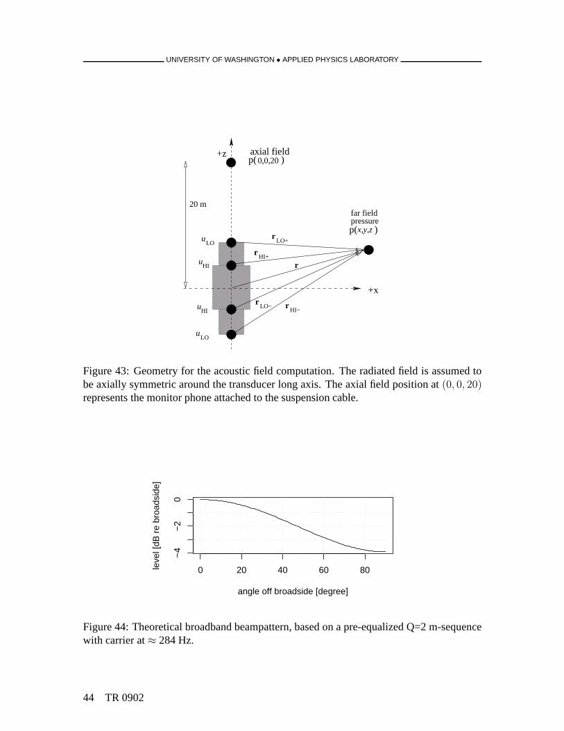
UNIVERSITY OF WASHINGTON • APPLIED PHYSICS LABORATORY
x,y,zp( )
0,0,20p( )
uLO
uLO
uHI
uHI
rHI+
rLO+
rHI−
rLO−
20 m
axial field+z
+x
far fieldpressure
r
Figure 43: Geometry for the acoustic field computation. The radiated field is assumed tobe axially symmetric around the transducer long axis. The axial field position at(0, 0, 20)represents the monitor phone attached to the suspension cable.
0 20 40 60 80
−4
−2
0
angle off broadside [degree]
leve
l [dB
re
broa
dsid
e]
Figure 44: Theoretical broadband beampattern, based on a pre-equalized Q=2 m-sequencewith carrier at≈ 284 Hz.
44 TR 0902
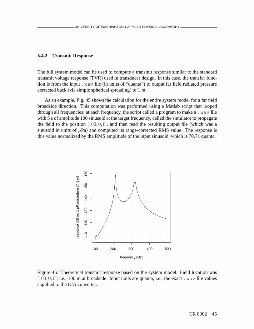
UNIVERSITY OF WASHINGTON • APPLIED PHYSICS LABORATORY
5.4.2 Transmit Response
The full system model can be used to compute a transmit response similar to the standardtransmit voltage response (TVR) used in transducer design.In this case, the transfer func-tion is from the input.wav file (in units of “quanta”) to output far field radiated pressurecorrected back (via simple spherical spreading) to 1 m.
As an example, Fig. 45 shows the calculation for the entire system model for a far fieldbroadside direction. This computation was performed usinga Matlab script that loopedthrough all frequencies; at each frequency, the script called a program to make a.wav filewith 5 s of amplitude 100 sinusoid at the target frequency, called the simulator to propagatethe field to the position[100, 0, 0], and then read the resulting output file (which was asinusoid in units ofµPa) and computed its range-corrected RMS value. The response isthis value normalized by the RMS amplitude of the input sinusoid, which is 70.71 quanta.
100 200 300 400 500
110
120
130
140
150
160
frequency [Hz]
resp
onse
[dB
re:
1 µ
Pa/
quan
tum
@ 1
m]
Figure 45: Theoretical transmit response based on the system model. Field location was[100, 0, 0], i.e., 100 m at broadside. Input units are quanta, i.e., the exact.wav file valuessupplied to the D/A converter.
TR 0902 45
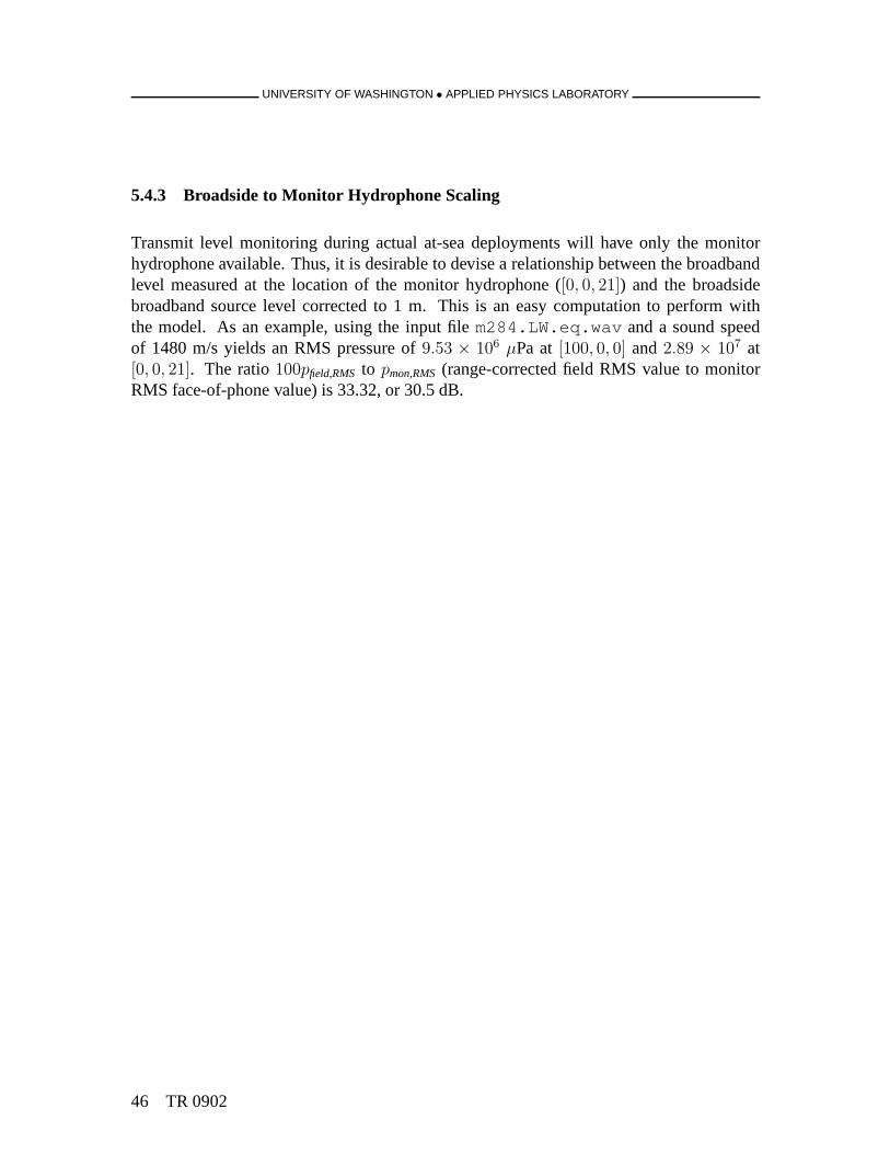
UNIVERSITY OF WASHINGTON • APPLIED PHYSICS LABORATORY
5.4.3 Broadside to Monitor Hydrophone Scaling
Transmit level monitoring during actual at-sea deployments will have only the monitorhydrophone available. Thus, it is desirable to devise a relationship between the broadbandlevel measured at the location of the monitor hydrophone ([0, 0, 21]) and the broadsidebroadband source level corrected to 1 m. This is an easy computation to perform withthe model. As an example, using the input filem284.LW.eq.wav and a sound speedof 1480 m/s yields an RMS pressure of9.53 × 106 µPa at[100, 0, 0] and2.89 × 107 at[0, 0, 21]. The ratio100pfield,RMS to pmon,RMS(range-corrected field RMS value to monitorRMS face-of-phone value) is 33.32, or 30.5 dB.
46 TR 0902
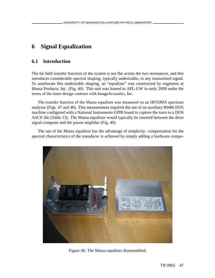
UNIVERSITY OF WASHINGTON • APPLIED PHYSICS LABORATORY
6 Signal Equalization
6.1 Introduction
The far field transfer function of the system is not flat acrossthe two resonances, and thisintroduces considerable spectral shaping, typically undesirable, to any transmitted signal.To ameliorate this undesirable shaping, an “equalizer” wasconstructed by engineers atMassa Products, Inc. (Fig. 46). This unit was loaned to APL-UW in early 2008 under theterms of the tuner design contract with ImageAcoustics, Inc.
The transfer function of the Massa equalizer was measured onan HP3589A spectrumanalyzer (Figs. 47 and 48). This measurement required the use of an auxiliary 80486 DOSmachine configured with a National Instruments GPIB board tocapture the trace to a DOSASCII file (Table 13). The Massa equalizer would typically beinserted between the drivesignal computer and the power amplifier (Fig. 49).
The use of the Massa equalizer has the advantage of simplicity: compensation for thespectral characteristics of the transducer is achieved by simply adding a hardware compo-
Figure 46: The Massa equalizer disassembled.
TR 0902 47
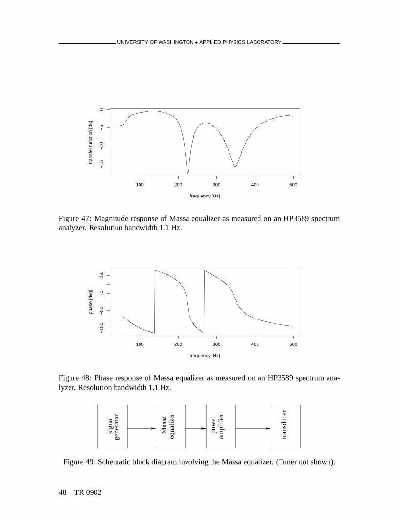
UNIVERSITY OF WASHINGTON • APPLIED PHYSICS LABORATORY
100 200 300 400 500
−15
−10
−5
0
frequency [Hz]
tran
sfer
func
tion
[dB
]
Figure 47: Magnitude response of Massa equalizer as measured on an HP3589 spectrumanalyzer. Resolution bandwidth 1.1 Hz.
100 200 300 400 500
−15
0−
5050
150
frequency [Hz]
phas
e [d
eg]
Figure 48: Phase response of Massa equalizer as measured on an HP3589 spectrum ana-lyzer. Resolution bandwidth 1.1 Hz.
gene
rato
rsi
gnal
Mas
sa
pow
er
tran
sduc
er
equa
lizer
ampl
ifier
Figure 49: Schematic block diagram involving the Massa equalizer. (Tuner not shown).
48 TR 0902

UNIVERSITY OF WASHINGTON • APPLIED PHYSICS LABORATORY
command purposeibic starts the interactive sessionibdev 0 19 0 13 1 0 opens a device, connects to the analyzeribwrt "DISP:RES D1" move trace in D1 register to trace Aibwrt "FORM:DATA ASC,7" set data format to ASCII, 7 sig. digitsibwrt "TRAC:DATA?" queues trace A data for retrievalibrdf "FOO.DAT" transfers data from analyzer to DOS fileibonl 0 closes the device
Table 13: AT-GPIB commands for retrieving trace data from the HP3589A.
nent into the signal circuit. The drawback of this approach is that the model for the entiresystem now requires a model for the Massa equalizer, which was not provided.
The alternative described below is to construct a “pre-equalizer” filter to pre-filter thedrive signal. This filter is implemented in the frequency domain. The advantage is thatthe system model developed previously need not be modified, and, further, that the filtercan be made to compensate nearly exactly for the hardware response (when SNR is high.)The disadvantage, primarily for the frequency domain filter, is that streaming operation ofan original waveform through the filter is not possible without recourse to a more complexsignal processing algorithm (such as an overlap-and-save methodology).
6.2 Theory
The equalizer filter can be developed using concepts from Wiener filter theory, where a sig-nalX, after possibly passing through some signal conditioning,is received in the presenceof additive noiseN (Fig. 50). Let the acoustic field at the receiver be
P (r) = XDGH(r). (30)
Therefore, the received signal is
Y (r) = P (r)K + NK. (31)
The optimal filterK∗ is chosen to minimize the expected error betweenY (r) andP (r).This gives
K∗ =A|D|2(HG(r))∗SXX
|D|2|HG(r)|2SXX + SNN(32)
whereSXX is the spectrum of the original input signal,SNN is the autospectrum of theadditive noise, andA is a user-adjustable scaling factor. Using simplySXX → |X|2 and
TR 0902 49
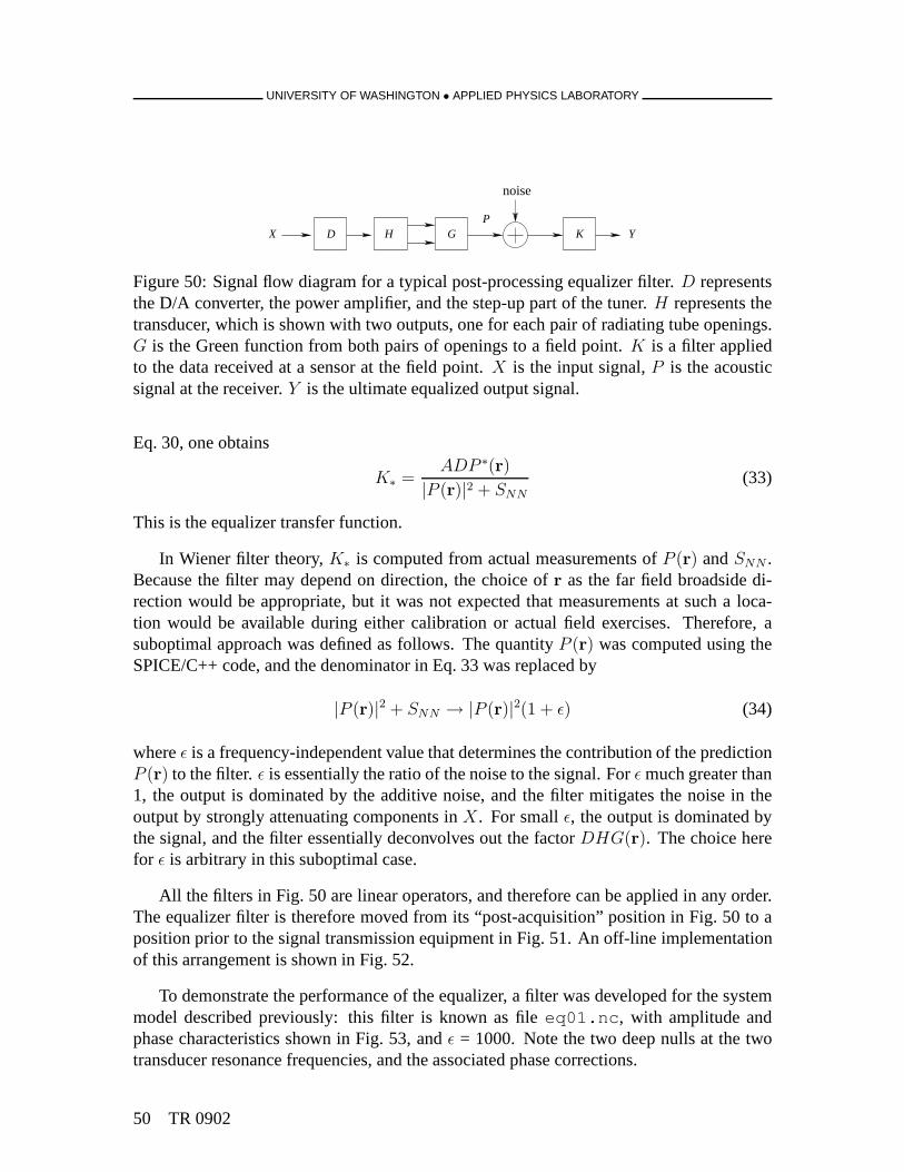
UNIVERSITY OF WASHINGTON • APPLIED PHYSICS LABORATORY
YKGHD
noise
XP
Figure 50: Signal flow diagram for a typical post-processingequalizer filter.D representsthe D/A converter, the power amplifier, and the step-up part of the tuner.H represents thetransducer, which is shown with two outputs, one for each pair of radiating tube openings.G is the Green function from both pairs of openings to a field point. K is a filter appliedto the data received at a sensor at the field point.X is the input signal,P is the acousticsignal at the receiver.Y is the ultimate equalized output signal.
Eq. 30, one obtains
K∗ =ADP ∗(r)
|P (r)|2 + SNN(33)
This is the equalizer transfer function.
In Wiener filter theory,K∗ is computed from actual measurements ofP (r) andSNN .Because the filter may depend on direction, the choice ofr as the far field broadside di-rection would be appropriate, but it was not expected that measurements at such a loca-tion would be available during either calibration or actualfield exercises. Therefore, asuboptimal approach was defined as follows. The quantityP (r) was computed using theSPICE/C++ code, and the denominator in Eq. 33 was replaced by
|P (r)|2 + SNN → |P (r)|2(1 + ǫ) (34)
whereǫ is a frequency-independent value that determines the contribution of the predictionP (r) to the filter.ǫ is essentially the ratio of the noise to the signal. Forǫ much greater than1, the output is dominated by the additive noise, and the filter mitigates the noise in theoutput by strongly attenuating components inX. For smallǫ, the output is dominated bythe signal, and the filter essentially deconvolves out the factor DHG(r). The choice herefor ǫ is arbitrary in this suboptimal case.
All the filters in Fig. 50 are linear operators, and thereforecan be applied in any order.The equalizer filter is therefore moved from its “post-acquisition” position in Fig. 50 to aposition prior to the signal transmission equipment in Fig.51. An off-line implementationof this arrangement is shown in Fig. 52.
To demonstrate the performance of the equalizer, a filter wasdeveloped for the systemmodel described previously: this filter is known as fileeq01.nc, with amplitude andphase characteristics shown in Fig. 53, andǫ = 1000. Note the two deep nulls at the twotransducer resonance frequencies, and the associated phase corrections.
50 TR 0902
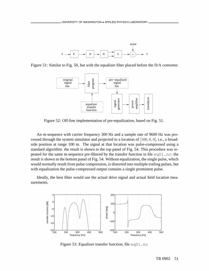
UNIVERSITY OF WASHINGTON • APPLIED PHYSICS LABORATORY
GHD
noise
KX Y
Figure 51: Similar to Fig. 50, but with the equalizer filter placed before the D/A converter.
pre−equalized
filesignal
tran
sduc
er
ampl
ifier
pow
er
gene
rato
rsi
gnal
filesignal
original
functiontransfer
equalizer
filte
rpr
ogra
m
Figure 52: Off-line implementation of pre-equalization, based on Fig. 51.
An m-sequence with carrier frequency 300 Hz and a sample rateof 9600 Hz was pro-cessed through the system simulator and projected to a location of [100, 0, 0], i.e., a broad-side position at range 100 m. The signal at that location was pulse-compressed using astandard algorithm: the result is shown in the top panel of Fig. 54. This procedure was re-peated for the same m-sequence pre-filtered by the transfer function in fileeq01.nc: theresult is shown in the bottom panel of Fig. 54. Without equalization, the single pulse, whichwould normally result from pulse compression, is distortedinto multiple trailing pulses, butwith equalization the pulse-compressed output contains a single prominent pulse.
Ideally, the best filter would use the actual drive signal andactual field location mea-surements.
100 200 300 400 500−20
−15
−10
−5
0
5
frequency [Hz]
tran
sfer
func
tion
[dB
]
100 200 300 400 500−200
−100
0
100
200
frequency [Hz]
phas
e [d
eg]
Figure 53: Equalizer transfer function, fileeq01.nc
TR 0902 51
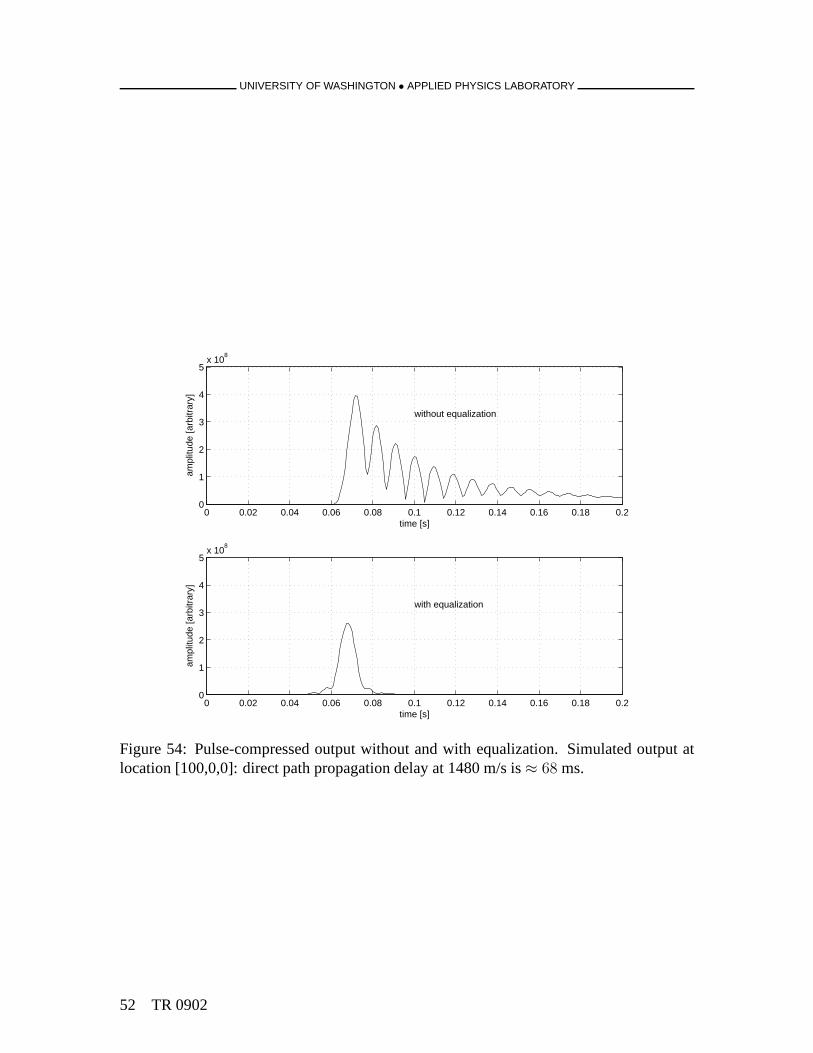
UNIVERSITY OF WASHINGTON • APPLIED PHYSICS LABORATORY
0 0.02 0.04 0.06 0.08 0.1 0.12 0.14 0.16 0.18 0.20
1
2
3
4
5x 10
8
time [s]
ampl
itude
[arb
itrar
y]
without equalization
0 0.02 0.04 0.06 0.08 0.1 0.12 0.14 0.16 0.18 0.20
1
2
3
4
5x 10
8
time [s]
ampl
itude
[arb
itrar
y]
with equalization
Figure 54: Pulse-compressed output without and with equalization. Simulated output atlocation [100,0,0]: direct path propagation delay at 1480 m/s is≈ 68 ms.
52 TR 0902
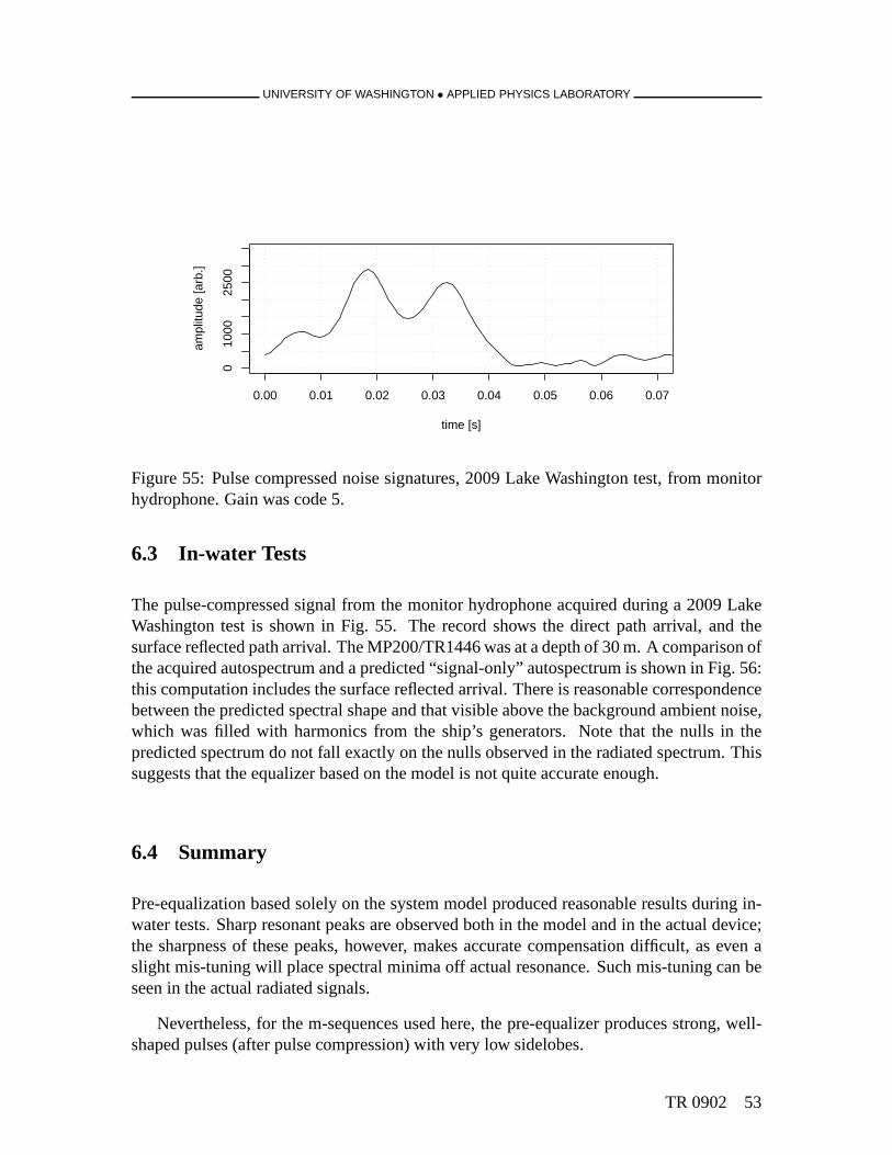
UNIVERSITY OF WASHINGTON • APPLIED PHYSICS LABORATORY
0.00 0.01 0.02 0.03 0.04 0.05 0.06 0.07
010
0025
00
time [s]
ampl
itude
[arb
.]
Figure 55: Pulse compressed noise signatures, 2009 Lake Washington test, from monitorhydrophone. Gain was code 5.
6.3 In-water Tests
The pulse-compressed signal from the monitor hydrophone acquired during a 2009 LakeWashington test is shown in Fig. 55. The record shows the direct path arrival, and thesurface reflected path arrival. The MP200/TR1446 was at a depth of 30 m. A comparison ofthe acquired autospectrum and a predicted “signal-only” autospectrum is shown in Fig. 56:this computation includes the surface reflected arrival. There is reasonable correspondencebetween the predicted spectral shape and that visible abovethe background ambient noise,which was filled with harmonics from the ship’s generators. Note that the nulls in thepredicted spectrum do not fall exactly on the nulls observedin the radiated spectrum. Thissuggests that the equalizer based on the model is not quite accurate enough.
6.4 Summary
Pre-equalization based solely on the system model producedreasonable results during in-water tests. Sharp resonant peaks are observed both in the model and in the actual device;the sharpness of these peaks, however, makes accurate compensation difficult, as even aslight mis-tuning will place spectral minima off actual resonance. Such mis-tuning can beseen in the actual radiated signals.
Nevertheless, for the m-sequences used here, the pre-equalizer produces strong, well-shaped pulses (after pulse compression) with very low sidelobes.
TR 0902 53
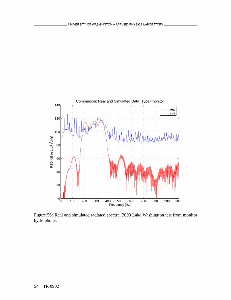
UNIVERSITY OF WASHINGTON • APPLIED PHYSICS LABORATORY
0 100 200 300 400 500 600 700 800 900 10000
20
40
60
80
100
120
140Comparison: Real and Simulated Data Type=monitor
Frequency [Hz]
PS
D [d
B r
e 1
µPa2 /H
z]
realsim
Figure 56: Real and simulated radiated spectra, 2009 Lake Washington test from monitorhydrophone.
54 TR 0902

UNIVERSITY OF WASHINGTON • APPLIED PHYSICS LABORATORY
Pre-equalizing a very long original waveform, or a streaming signal, would require amuch more advanced algorithm. For such a case a post-signal generator hardware filter,i.e., the Massa equalizer, is probably simpler.
TR 0902 55
UNIVERSITY OF WASHINGTON • APPLIED PHYSICS LABORATORY
7 The Philippine Sea Engineering Test / Pilot Study
7.1 Summary
For several decades, the Office of Naval Research has sponsored an international consor-tium of scientists to investigate deterministic and stochastic acoustic propagation at lowfrequencies over long ranges in the deep ocean. Most of these“blue water” experimentshave been conducted in the central North Pacific, where oceanographic processes are rel-atively benign. The natural progression for these studies is to determine whether and towhat extent the models and predictions developed during these efforts apply in a regionwith more vigorous oceanic processes.
This scientific consortium identified the Philippine Sea as areasonable venue for thiseffort. This region is bounded to the south by the North Equatorial Current (NEC) and to thewest by the Kuroshio. Mesoscale structures propagate westward into the basin and collidewith eddies spun off from the Kuroshio, creating energetic and complicated oceanography.
The primary scientific experiment is planned for 2010–2011,and involves a consider-able number of new systems. To mitigate the risk of deployingnew systems, the groupconducted a pilot study/engineering test in the same operating environment in March–May2009.
The geographical region of operations and the assets deployed are shown in Fig. 57.These include:
1. An autonomous transceiver mooring (T1). This unit was oneof six under refurbish-ment for the 2010–2011 experiment, and was deployed at the design position for theT1 mooring.
2. A distributed vertical line array (VLA). In 2009 this was a5000-m partially populateddevelopment version of a system targeted for the main experiment. This was locatedat the design intersection of two transects between severalautonomous transceivermoorings scheduled for the 2010–2011 experiment.
3. Ship-suspended stationary operations along the path between T1 and the VLA. Sta-tionary operations listed herein occurred at ship stops SS45 and SS107.
The MP200/TR1446 was freighted to Kao-Hsiung, Taiwan, in March 2009, and liftedaboard the R/VMelville for use during the ONR 2009 Philippine Sea engineering test /pilot study.
56 TR 0902

UNIVERSITY OF WASHINGTON • APPLIED PHYSICS LABORATORY
124˚
124˚
126˚
126˚
128˚
128˚
20˚ 20˚
22˚ 22˚
24˚ 24˚
T1
T6
VLA
SS45
SS107
Figure 57: Geographical context for the Philippine Sea 2009exercise. APL-UW deployedthe MP200/TR1446 at ship stops SS45 and SS107.
TR 0902 57
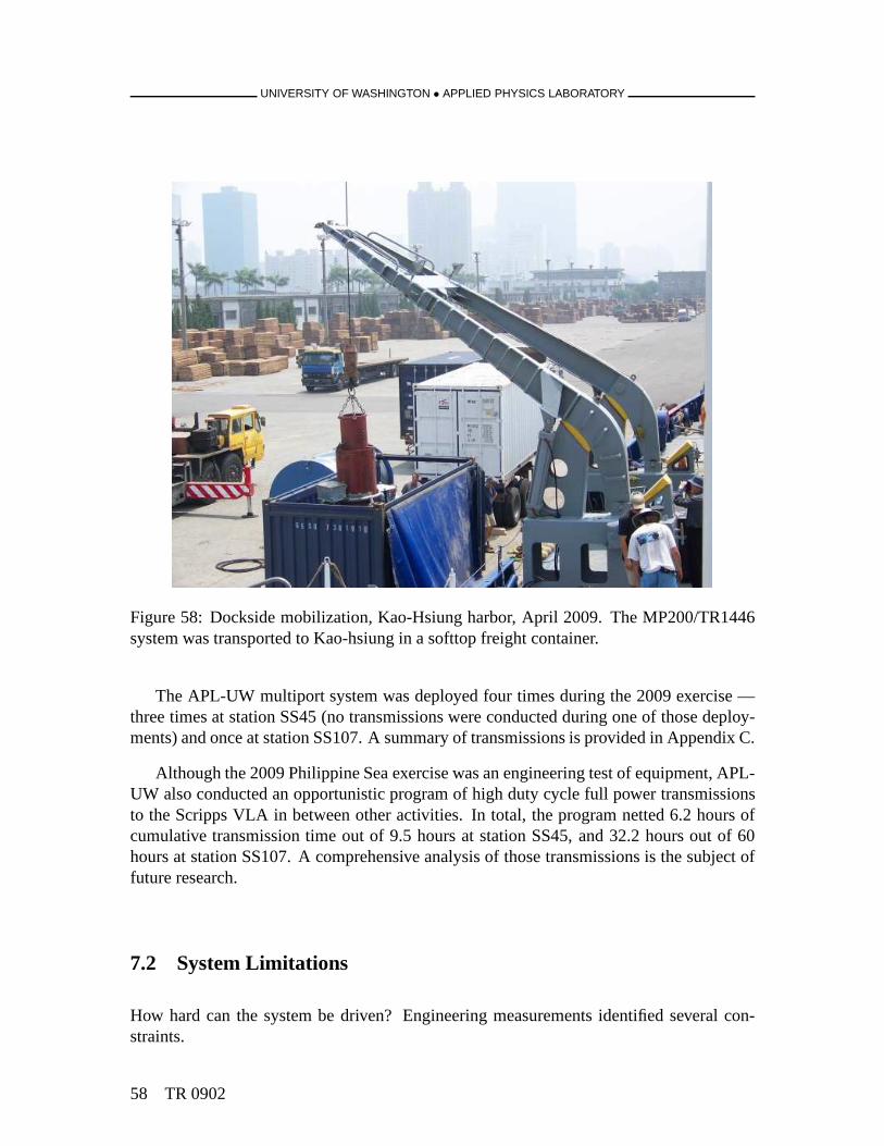
UNIVERSITY OF WASHINGTON • APPLIED PHYSICS LABORATORY
Figure 58: Dockside mobilization, Kao-Hsiung harbor, April 2009. The MP200/TR1446system was transported to Kao-hsiung in a softtop freight container.
The APL-UW multiport system was deployed four times during the 2009 exercise —three times at station SS45 (no transmissions were conducted during one of those deploy-ments) and once at station SS107. A summary of transmissionsis provided in Appendix C.
Although the 2009 Philippine Sea exercise was an engineering test of equipment, APL-UW also conducted an opportunistic program of high duty cycle full power transmissionsto the Scripps VLA in between other activities. In total, theprogram netted 6.2 hours ofcumulative transmission time out of 9.5 hours at station SS45, and 32.2 hours out of 60hours at station SS107. A comprehensive analysis of those transmissions is the subject offuture research.
7.2 System Limitations
How hard can the system be driven? Engineering measurementsidentified several con-straints.
58 TR 0902
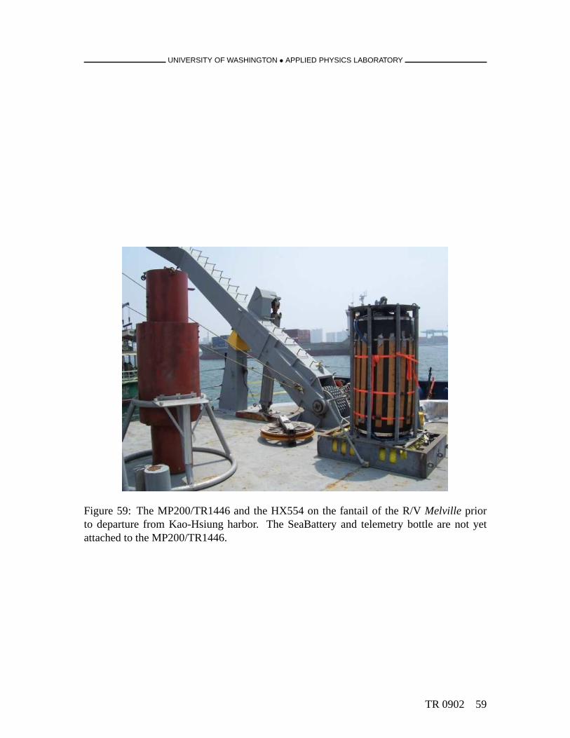
UNIVERSITY OF WASHINGTON • APPLIED PHYSICS LABORATORY
Figure 59: The MP200/TR1446 and the HX554 on the fantail of the R/V Melville priorto departure from Kao-Hsiung harbor. The SeaBattery and telemetry bottle are not yetattached to the MP200/TR1446.
TR 0902 59
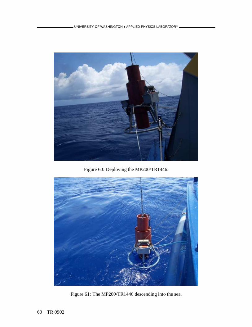
UNIVERSITY OF WASHINGTON • APPLIED PHYSICS LABORATORY
Figure 60: Deploying the MP200/TR1446.
Figure 61: The MP200/TR1446 descending into the sea.
60 TR 0902

UNIVERSITY OF WASHINGTON • APPLIED PHYSICS LABORATORY
Figure 62: Recovering the MP200/TR1446. Two hand lines and two lines attached to airtuggers were used to control the system.
Figure 63: Attaching the monitor hydrophone and its bungy mounting frame to the suspen-sion cable over the stern of the R/VMelville during deployment.
TR 0902 61
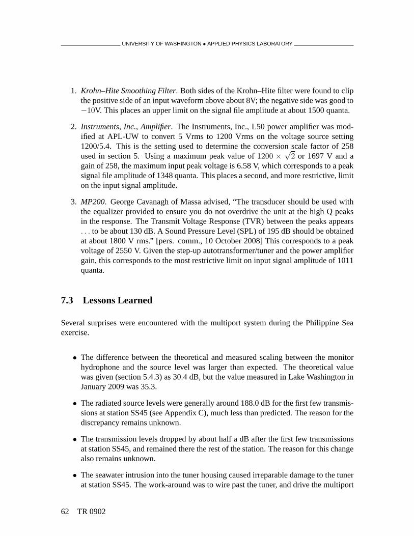
UNIVERSITY OF WASHINGTON • APPLIED PHYSICS LABORATORY
1. Krohn–Hite Smoothing Filter. Both sides of the Krohn–Hite filter were found to clipthe positive side of an input waveform above about 8V; the negative side was good to−10V. This places an upper limit on the signal file amplitude at about 1500 quanta.
2. Instruments, Inc., Amplifier. The Instruments, Inc., L50 power amplifier was mod-ified at APL-UW to convert 5 Vrms to 1200 Vrms on the voltage source setting1200/5.4. This is the setting used to determine the conversion scale factor of 258used in section 5. Using a maximum peak value of1200 ×
√2 or 1697 V and a
gain of 258, the maximum input peak voltage is 6.58 V, which corresponds to a peaksignal file amplitude of 1348 quanta. This places a second, and more restrictive, limiton the input signal amplitude.
3. MP200. George Cavanagh of Massa advised, “The transducer should be used withthe equalizer provided to ensure you do not overdrive the unit at the high Q peaksin the response. The Transmit Voltage Response (TVR) between the peaks appears. . . to be about 130 dB. A Sound Pressure Level (SPL) of 195 dB should be obtainedat about 1800 V rms.” [pers. comm., 10 October 2008] This corresponds to a peakvoltage of 2550 V. Given the step-up autotransformer/tunerand the power amplifiergain, this corresponds to the most restrictive limit on input signal amplitude of 1011quanta.
7.3 Lessons Learned
Several surprises were encountered with the multiport system during the Philippine Seaexercise.
• The difference between the theoretical and measured scaling between the monitorhydrophone and the source level was larger than expected. The theoretical valuewas given (section 5.4.3) as 30.4 dB, but the value measured in Lake Washington inJanuary 2009 was 35.3.
• The radiated source levels were generally around 188.0 dB for the first few transmis-sions at station SS45 (see Appendix C), much less than predicted. The reason for thediscrepancy remains unknown.
• The transmission levels dropped by about half a dB after the first few transmissionsat station SS45, and remained there the rest of the station. The reason for this changealso remains unknown.
• The seawater intrusion into the tuner housing caused irreparable damage to the tunerat station SS45. The work-around was to wire past the tuner, and drive the multiport
62 TR 0902
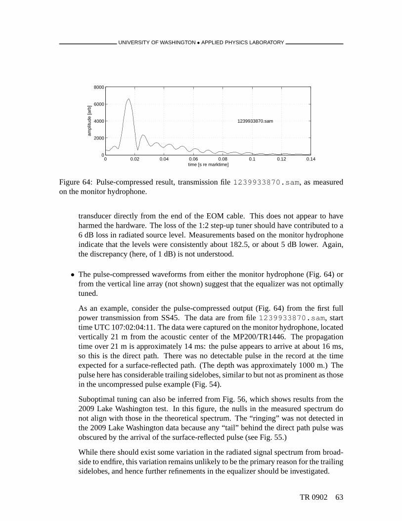
UNIVERSITY OF WASHINGTON • APPLIED PHYSICS LABORATORY
0 0.02 0.04 0.06 0.08 0.1 0.12 0.140
2000
4000
6000
8000
time [s re marktime]
ampl
itude
[arb
]
1239933870.sam
Figure 64: Pulse-compressed result, transmission file1239933870.sam, as measuredon the monitor hydrophone.
transducer directly from the end of the EOM cable. This does not appear to haveharmed the hardware. The loss of the 1:2 step-up tuner shouldhave contributed to a6 dB loss in radiated source level. Measurements based on themonitor hydrophoneindicate that the levels were consistently about 182.5, or about 5 dB lower. Again,the discrepancy (here, of 1 dB) is not understood.
• The pulse-compressed waveforms from either the monitor hydrophone (Fig. 64) orfrom the vertical line array (not shown) suggest that the equalizer was not optimallytuned.
As an example, consider the pulse-compressed output (Fig. 64) from the first fullpower transmission from SS45. The data are from file1239933870.sam, starttime UTC 107:02:04:11. The data were captured on the monitorhydrophone, locatedvertically 21 m from the acoustic center of the MP200/TR1446. The propagationtime over 21 m is approximately 14 ms: the pulse appears to arrive at about 16 ms,so this is the direct path. There was no detectable pulse in the record at the timeexpected for a surface-reflected path. (The depth was approximately 1000 m.) Thepulse here has considerable trailing sidelobes, similar tobut not as prominent as thosein the uncompressed pulse example (Fig. 54).
Suboptimal tuning can also be inferred from Fig. 56, which shows results from the2009 Lake Washington test. In this figure, the nulls in the measured spectrum donot align with those in the theoretical spectrum. The “ringing” was not detected inthe 2009 Lake Washington data because any “tail” behind the direct path pulse wasobscured by the arrival of the surface-reflected pulse (see Fig. 55.)
While there should exist some variation in the radiated signal spectrum from broad-side to endfire, this variation remains unlikely to be the primary reason for the trailingsidelobes, and hence further refinements in the equalizer should be investigated.
TR 0902 63

UNIVERSITY OF WASHINGTON • APPLIED PHYSICS LABORATORY
It is no surprise that the performance predictions made withthe system model werenot completely accurate. Many simplifying approximationswere made to establish thesystem model. Nevertheless, the discrepancies were not severe considering no full or evenmoderate power calibration was conducted with the fully assembled system. Without such acalibration, the effects on acoustic parameters such as resonance frequencies and broadsideradiated source level of various system-level mechanical issues, such as the tuner mass andSeaBattery mass mounted at the transducer equator, remain unknown.
In spite of all the engineering approximations, the multiport system provided manyhours of usable acoustic data during the 2009 Philippine Seaexercise. Further refinementsare anticipated for future experiments.
64 TR 0902
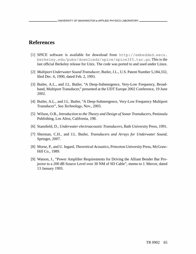
UNIVERSITY OF WASHINGTON • APPLIED PHYSICS LABORATORY
References
[1] SPICE software is available for download fromhttp://embedded.eecs.berkeley.edu/pubs/downloads/spice/spice3f5.tar.gz. This is thelast official Berkeley release for Unix. The code was ported to and used under Linux.
[2] Multiport Underwater Sound Transducer, Butler, J.L., U.S. Patent Number 5,184,332,filed Dec. 6, 1990, dated Feb. 2, 1993.
[3] Butler, A.L., and J.L. Butler, “A Deep-Submergence, Very-Low Frequency, Broad-band, Multiport Transducer,” presented at the UDT Europe 2002 Conference, 19 June2002.
[4] Butler, A.L., and J.L. Butler, “A Deep-Submergence, Very-Low Frequency MultiportTransducer”,Sea Technology, Nov., 2003.
[5] Wilson, O.B.,Introduction to the Theory and Design of Sonar Transducers, PeninsulaPublishing, Los Altos, California, 198.
[6] Stansfield, D.,Underwater electroacoustic Transducers, Bath University Press, 1991.
[7] Sherman, C.H., and J.L. Butler,Transducers and Arrays for Underwater Sound,Springer, 2007.
[8] Morse, P., and U. Ingard,Theoretical Acoustics, Princeton University Press, McGraw-Hill Co., 1989.
[9] Watson, J., “Power Amplifier Requirements for Driving the Alliant Bender Bar Pro-jector to a 200 dB Source Level over 30 NM of SD Cable”, memo to J. Mercer, dated13 January 1993.
TR 0902 65
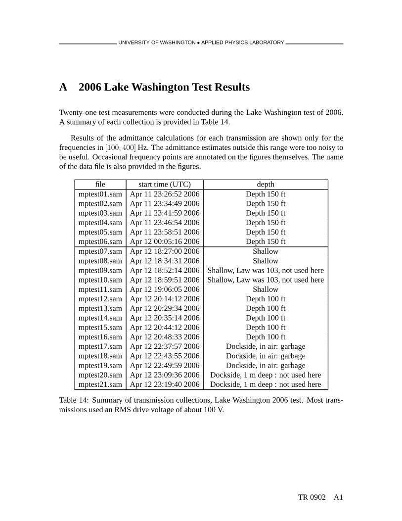
UNIVERSITY OF WASHINGTON • APPLIED PHYSICS LABORATORY
A 2006 Lake Washington Test Results
Twenty-one test measurements were conducted during the Lake Washington test of 2006.A summary of each collection is provided in Table 14.
Results of the admittance calculations for each transmission are shown only for thefrequencies in[100, 400] Hz. The admittance estimates outside this range were too noisy tobe useful. Occasional frequency points are annotated on thefigures themselves. The nameof the data file is also provided in the figures.
file start time (UTC) depthmptest01.sam Apr 11 23:26:52 2006 Depth 150 ftmptest02.sam Apr 11 23:34:49 2006 Depth 150 ftmptest03.sam Apr 11 23:41:59 2006 Depth 150 ftmptest04.sam Apr 11 23:46:54 2006 Depth 150 ftmptest05.sam Apr 11 23:58:51 2006 Depth 150 ftmptest06.sam Apr 12 00:05:16 2006 Depth 150 ftmptest07.sam Apr 12 18:27:00 2006 Shallowmptest08.sam Apr 12 18:34:31 2006 Shallowmptest09.sam Apr 12 18:52:14 2006 Shallow, Law was 103, not used heremptest10.sam Apr 12 18:59:51 2006 Shallow, Law was 103, not used heremptest11.sam Apr 12 19:06:05 2006 Shallowmptest12.sam Apr 12 20:14:12 2006 Depth 100 ftmptest13.sam Apr 12 20:29:34 2006 Depth 100 ftmptest14.sam Apr 12 20:35:14 2006 Depth 100 ftmptest15.sam Apr 12 20:44:12 2006 Depth 100 ftmptest16.sam Apr 12 20:48:33 2006 Depth 100 ftmptest17.sam Apr 12 22:37:57 2006 Dockside, in air: garbagemptest18.sam Apr 12 22:43:55 2006 Dockside, in air: garbagemptest19.sam Apr 12 22:49:59 2006 Dockside, in air: garbagemptest20.sam Apr 12 23:09:36 2006 Dockside, 1 m deep : not used heremptest21.sam Apr 12 23:19:40 2006 Dockside, 1 m deep : not used here
Table 14: Summary of transmission collections, Lake Washington 2006 test. Most trans-missions used an RMS drive voltage of about 100 V.
TR 0902 A1
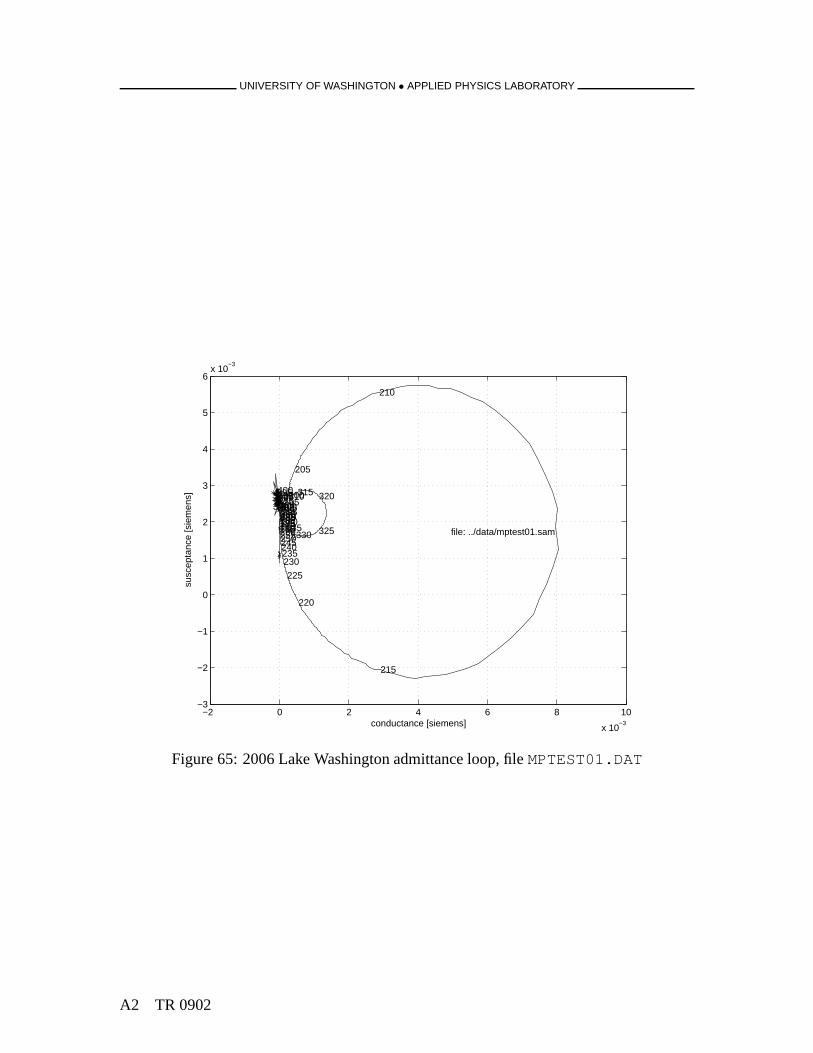
UNIVERSITY OF WASHINGTON • APPLIED PHYSICS LABORATORY
−2 0 2 4 6 8 10
x 10−3
−3
−2
−1
0
1
2
3
4
5
6x 10
−3
conductance [siemens]
susc
epta
nce
[sie
men
s]
180185190195
200
205
210
215
220
225
230235240245250255260265270275280285290295300305
310315 320
325330335
340345350355360365370375380385390395400
file: ../data/mptest01.sam
Figure 65: 2006 Lake Washington admittance loop, fileMPTEST01.DAT
A2 TR 0902
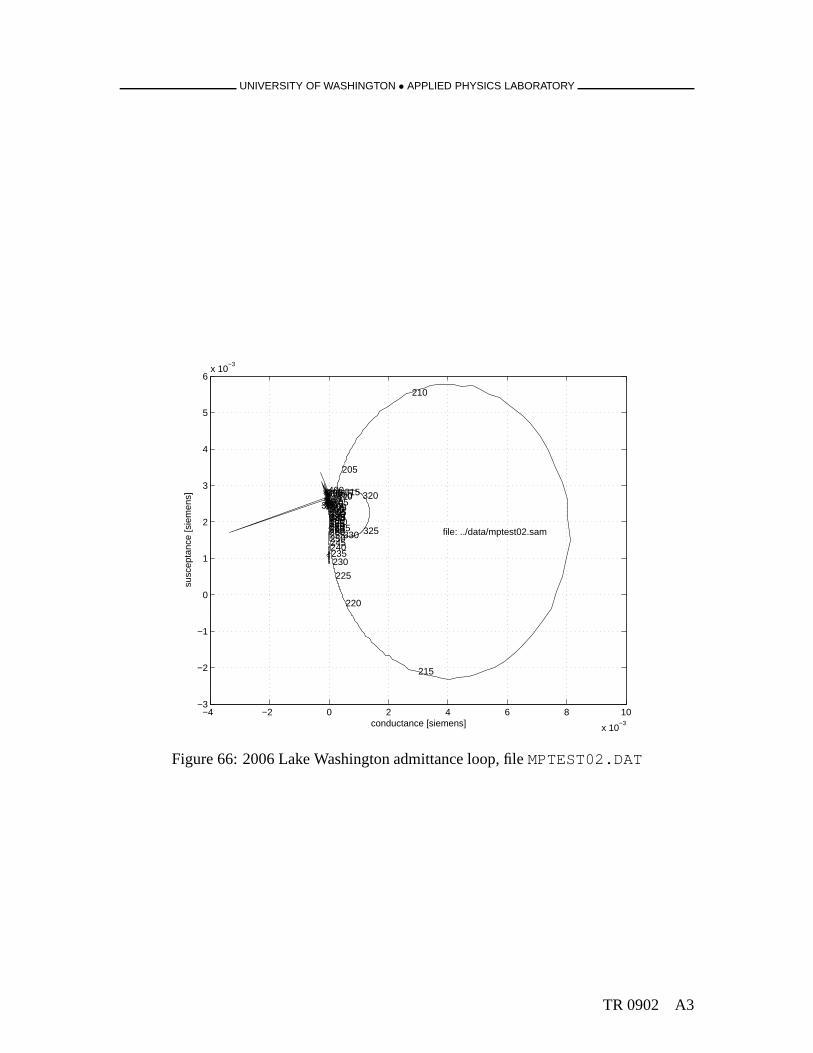
UNIVERSITY OF WASHINGTON • APPLIED PHYSICS LABORATORY
−4 −2 0 2 4 6 8 10
x 10−3
−3
−2
−1
0
1
2
3
4
5
6x 10
−3
conductance [siemens]
susc
epta
nce
[sie
men
s]
180185190195
200
205
210
215
220
225
230235240245250255260265270275280285290295300305
310315 320
325330335
340345350355360365370375380385390395400
file: ../data/mptest02.sam
Figure 66: 2006 Lake Washington admittance loop, fileMPTEST02.DAT
TR 0902 A3

UNIVERSITY OF WASHINGTON • APPLIED PHYSICS LABORATORY
−2 0 2 4 6 8 10
x 10−3
−3
−2
−1
0
1
2
3
4
5
6x 10
−3
conductance [siemens]
susc
epta
nce
[sie
men
s]
180185190195
200
205
210
215
220
225
230235240245250255260265270275280285290295300305
310315 320
325330335
340345350355360365370375380385390395400
file: ../data/mptest03.sam
Figure 67: 2006 Lake Washington admittance loop, fileMPTEST03.DAT
A4 TR 0902
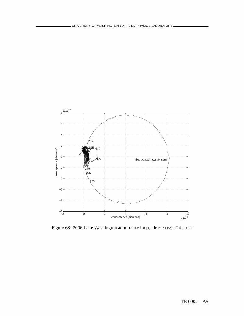
UNIVERSITY OF WASHINGTON • APPLIED PHYSICS LABORATORY
−2 0 2 4 6 8 10
x 10−3
−3
−2
−1
0
1
2
3
4
5
6x 10
−3
conductance [siemens]
susc
epta
nce
[sie
men
s]
180185190195
200
205
210
215
220
225
230235240245250255260265270275280285290295300305310315 320
325330335
340345350355360365370375380385390395400
file: ../data/mptest04.sam
Figure 68: 2006 Lake Washington admittance loop, fileMPTEST04.DAT
TR 0902 A5
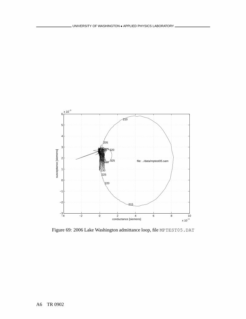
UNIVERSITY OF WASHINGTON • APPLIED PHYSICS LABORATORY
−4 −2 0 2 4 6 8 10
x 10−3
−3
−2
−1
0
1
2
3
4
5
6x 10
−3
conductance [siemens]
susc
epta
nce
[sie
men
s]
180185190195
200
205
210
215
220
225
230235240245250255260265270275280285290295300305310315 320
325330335
340345350355360365370375380385390395400
file: ../data/mptest05.sam
Figure 69: 2006 Lake Washington admittance loop, fileMPTEST05.DAT
A6 TR 0902
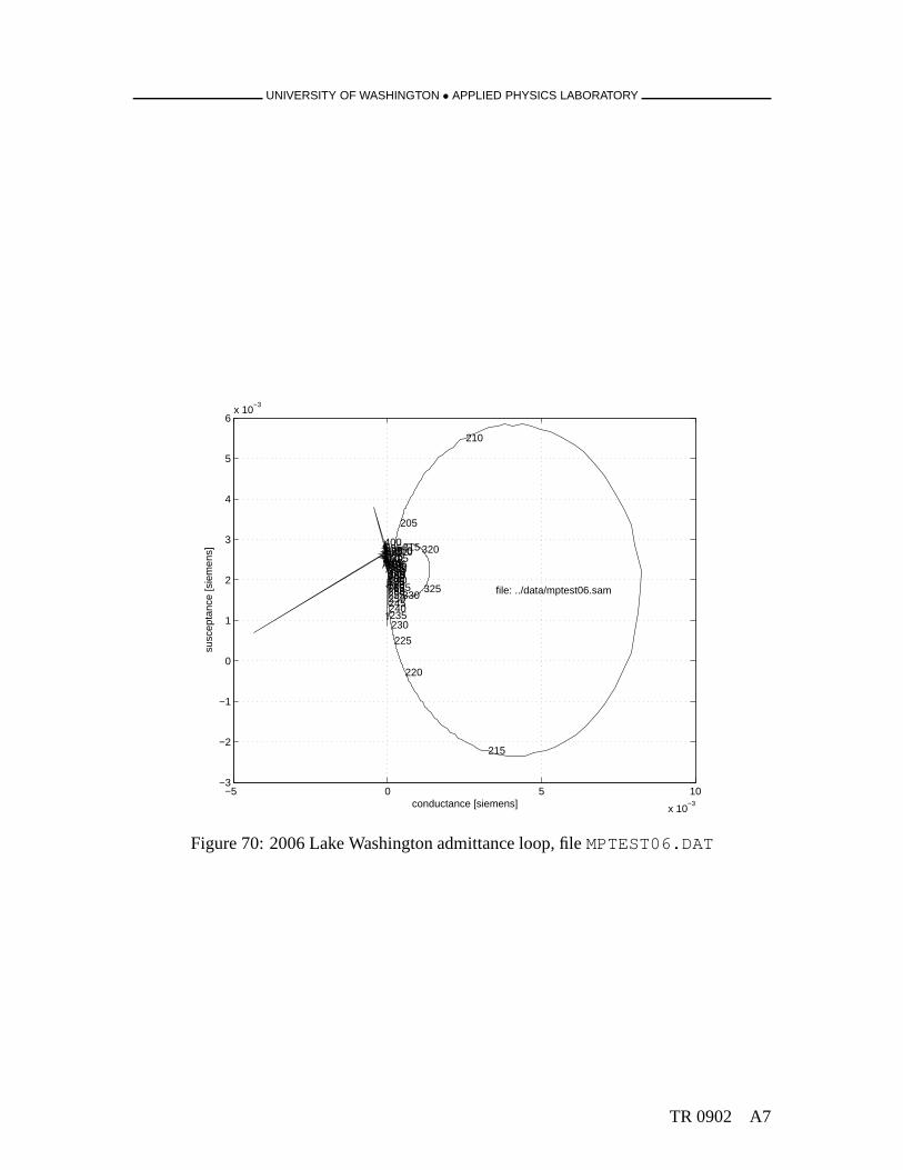
UNIVERSITY OF WASHINGTON • APPLIED PHYSICS LABORATORY
−5 0 5 10
x 10−3
−3
−2
−1
0
1
2
3
4
5
6x 10
−3
conductance [siemens]
susc
epta
nce
[sie
men
s]
180185190195
200
205
210
215
220
225
230235240245250255260265270275280285290295300305310315 320
325330
335340345350355360365370
375380385390395400
file: ../data/mptest06.sam
Figure 70: 2006 Lake Washington admittance loop, fileMPTEST06.DAT
TR 0902 A7
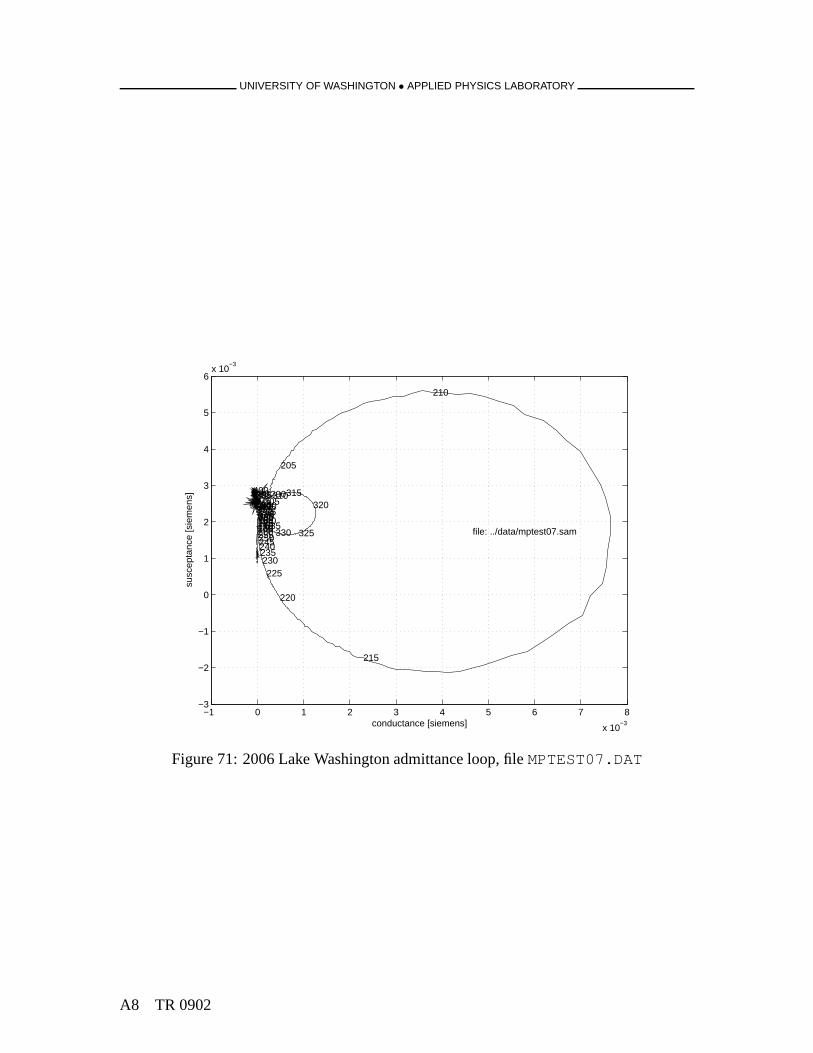
UNIVERSITY OF WASHINGTON • APPLIED PHYSICS LABORATORY
−1 0 1 2 3 4 5 6 7 8
x 10−3
−3
−2
−1
0
1
2
3
4
5
6x 10
−3
conductance [siemens]
susc
epta
nce
[sie
men
s]
180185190195
200
205
210
215
220
225230235240245250255260265270275280285290295300305
310315320
325330335340345350355360365370375380
385390395400
file: ../data/mptest07.sam
Figure 71: 2006 Lake Washington admittance loop, fileMPTEST07.DAT
A8 TR 0902

UNIVERSITY OF WASHINGTON • APPLIED PHYSICS LABORATORY
−1 0 1 2 3 4 5 6 7 8
x 10−3
−3
−2
−1
0
1
2
3
4
5
6x 10
−3
conductance [siemens]
susc
epta
nce
[sie
men
s]
180185190195
200
205
210
215
220
225230235240245250255260265270275280285290295300305
310315320
325330335
340345350355360365370375380385390395400
file: ../data/mptest08.sam
Figure 72: 2006 Lake Washington admittance loop, fileMPTEST08.DAT
TR 0902 A9

UNIVERSITY OF WASHINGTON • APPLIED PHYSICS LABORATORY
−2 0 2 4 6 8 10
x 10−3
−3
−2
−1
0
1
2
3
4
5
6x 10
−3
conductance [siemens]
susc
epta
nce
[sie
men
s]
180185190195
200
205
210
215
220
225
230235240245250255260265270275280285290295300305
310315320
325330335
340345350355360365370375380385390395400
file: ../data/mptest11.sam
Figure 73: 2006 Lake Washington admittance loop, fileMPTEST11.DAT
A10 TR 0902
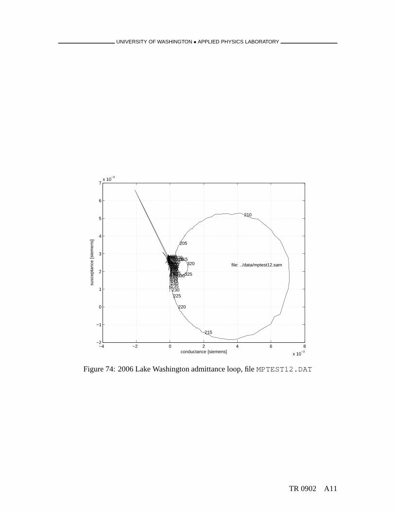
UNIVERSITY OF WASHINGTON • APPLIED PHYSICS LABORATORY
−4 −2 0 2 4 6 8
x 10−3
−2
−1
0
1
2
3
4
5
6
7x 10
−3
conductance [siemens]
susc
epta
nce
[sie
men
s]
180185190195
200
205
210
215
220
225230235240245250255260265270275280285290295300305310315
320
325330335340345350355360365370375380385390395400
file: ../data/mptest12.sam
Figure 74: 2006 Lake Washington admittance loop, fileMPTEST12.DAT
TR 0902 A11

UNIVERSITY OF WASHINGTON • APPLIED PHYSICS LABORATORY
−1 0 1 2 3 4 5 6 7 8
x 10−3
−2
−1
0
1
2
3
4
5
6x 10
−3
conductance [siemens]
susc
epta
nce
[sie
men
s]
180185190195
200
205
210
215
220
225
230235240245250255260265270275280285290295300305
310315320
325330335340
345350355360365370375380385390395400
file: ../data/mptest13.sam
Figure 75: 2006 Lake Washington admittance loop, fileMPTEST13.DAT
A12 TR 0902
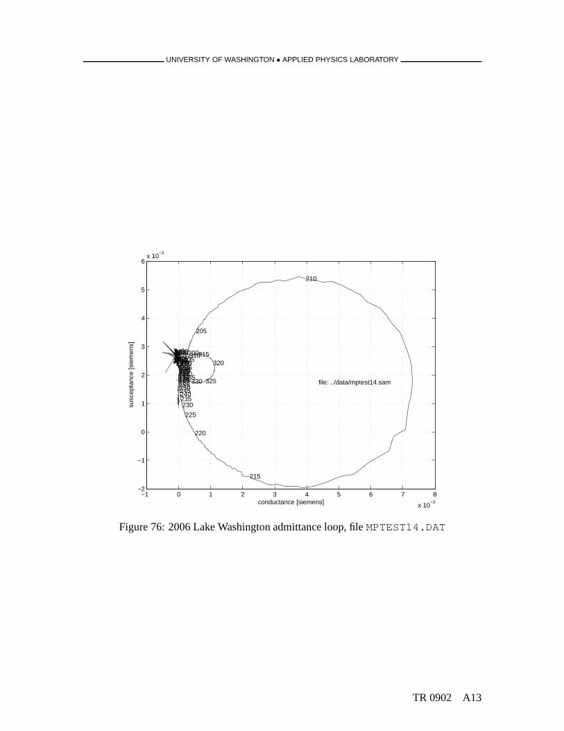
UNIVERSITY OF WASHINGTON • APPLIED PHYSICS LABORATORY
−1 0 1 2 3 4 5 6 7 8
x 10−3
−2
−1
0
1
2
3
4
5
6x 10
−3
conductance [siemens]
susc
epta
nce
[sie
men
s]
180185190195
200
205
210
215
220
225
230235240245250255260265270275280285290295300305
310315320
325330335340345350355360365370375380
385390395400
file: ../data/mptest14.sam
Figure 76: 2006 Lake Washington admittance loop, fileMPTEST14.DAT
TR 0902 A13
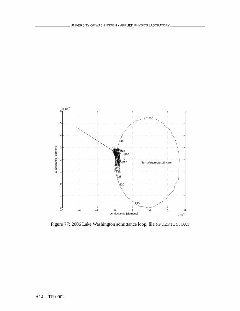
UNIVERSITY OF WASHINGTON • APPLIED PHYSICS LABORATORY
−6 −4 −2 0 2 4 6 8
x 10−3
−2
−1
0
1
2
3
4
5
6x 10
−3
conductance [siemens]
susc
epta
nce
[sie
men
s]
180185190195
200
205
210
215
220
225
230235240245250255260265270275280285290295300305
310315320
325330335340345350355360365370375380
385390395400
file: ../data/mptest15.sam
Figure 77: 2006 Lake Washington admittance loop, fileMPTEST15.DAT
A14 TR 0902
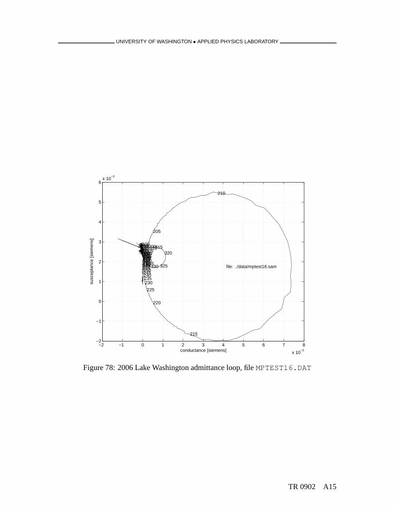
UNIVERSITY OF WASHINGTON • APPLIED PHYSICS LABORATORY
−2 −1 0 1 2 3 4 5 6 7 8
x 10−3
−2
−1
0
1
2
3
4
5
6x 10
−3
conductance [siemens]
susc
epta
nce
[sie
men
s]
180185190195
200
205
210
215
220
225
230235240245250255260265270275280285290295300305
310315320
325330335
340345350355360365370375380385390395400
file: ../data/mptest16.sam
Figure 78: 2006 Lake Washington admittance loop, fileMPTEST16.DAT
TR 0902 A15
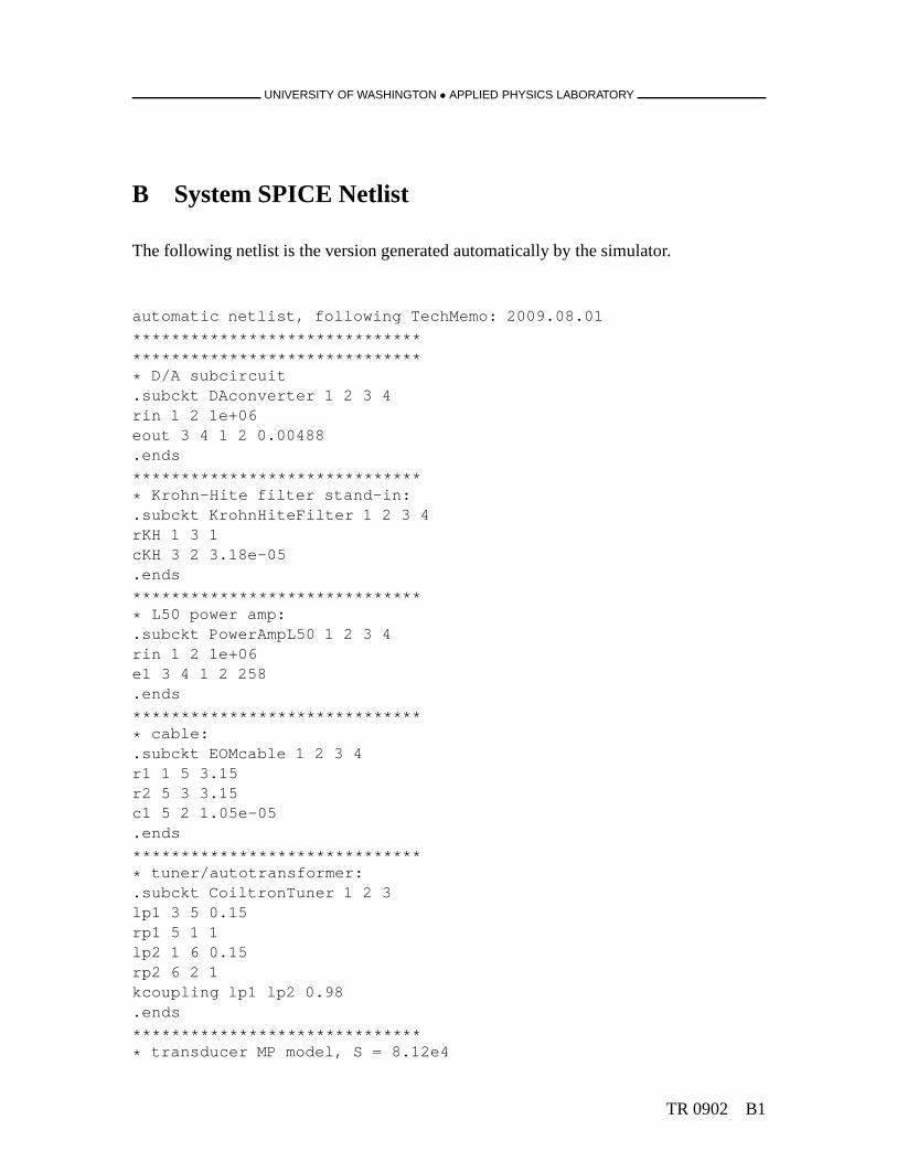
UNIVERSITY OF WASHINGTON • APPLIED PHYSICS LABORATORY
B System SPICE Netlist
The following netlist is the version generated automatically by the simulator.
automatic netlist, following TechMemo: 2009.08.01
************************************************************* D/A subcircuit.subckt DAconverter 1 2 3 4rin 1 2 1e+06eout 3 4 1 2 0.00488.ends
******************************* Krohn-Hite filter stand-in:.subckt KrohnHiteFilter 1 2 3 4rKH 1 3 1cKH 3 2 3.18e-05.ends
******************************* L50 power amp:.subckt PowerAmpL50 1 2 3 4rin 1 2 1e+06e1 3 4 1 2 258.ends
******************************* cable:.subckt EOMcable 1 2 3 4r1 1 5 3.15r2 5 3 3.15c1 5 2 1.05e-05.ends
******************************* tuner/autotransformer:.subckt CoiltronTuner 1 2 3lp1 3 5 0.15rp1 5 1 1lp2 1 6 0.15rp2 6 2 1kcoupling lp1 lp2 0.98.ends
******************************* transducer MP model, S = 8.12e4
TR 0902 B1
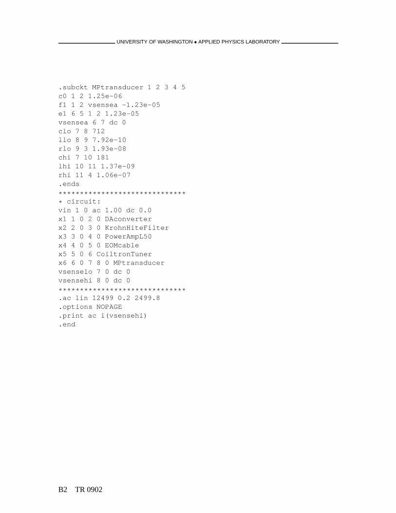
UNIVERSITY OF WASHINGTON • APPLIED PHYSICS LABORATORY
.subckt MPtransducer 1 2 3 4 5c0 1 2 1.25e-06f1 1 2 vsensea -1.23e-05e1 6 5 1 2 1.23e-05vsensea 6 7 dc 0clo 7 8 712llo 8 9 7.92e-10rlo 9 3 1.93e-08chi 7 10 181lhi 10 11 1.37e-09rhi 11 4 1.06e-07.ends
******************************* circuit:vin 1 0 ac 1.00 dc 0.0x1 1 0 2 0 DAconverterx2 2 0 3 0 KrohnHiteFilterx3 3 0 4 0 PowerAmpL50x4 4 0 5 0 EOMcablex5 5 0 6 CoiltronTunerx6 6 0 7 8 0 MPtransducervsenselo 7 0 dc 0vsensehi 8 0 dc 0
******************************.ac lin 12499 0.2 2499.8.options NOPAGE.print ac i(vsensehi).end
B2 TR 0902
UNIVERSITY OF WASHINGTON • APPLIED PHYSICS LABORATORY
C 2009 Philippine Sea Transmissions
C.1 Background
Signals were transmitted during the 2009 ONR Philippine SeaPilot Study/Engineering Testat two “ship stops,” SS45 and SS107. The total number of multiport system transmissionsat stations SS45 and SS107 were 19 and 214, respectively. Therespective total transmissiontimes were 6.2 hours spanning 9.5 hours and 32.3 hours spanning 60 hours.
A transmission file was generated for each transmission. Thestart time is given in theform YYY:HH:MM:SS where YYY is the yearday with January 1 being 001, all in UTC.The times listed below are the actual times of the first secondof transmission, as decodedfrom the IRIG channel. The marktime is 20 seconds later, and may be different by 1 secondfrom the target marktime recorded in the file header. (See below for explanation.) The rampin all cases is 20 seconds.
C.2 Station SS45
There were three deployments of the MP200/TR1446 at SS45:
1. From 4/17 00:00Z to 4/18 00:00Z (day 107). Scheduled transmissions were inter-rupted several times for heat build-up issues in the sciencevan. Transmissions wereaborted due to shorting in the underwater package. This was later determined tobe due to seawater in the transformer housing (oil expansionsystem tubing discon-nected, possibly in going through the air–sea interface in strong currents. )
2. From 4/20 02:00Z to 4/20 08:00Z (day 110). The second transmission was aborteddue to shorting in the underwater package. This was later determined to be a leak inthe splice: there was also possible damage to the autotransformer.
3. 4/24 (day 114). The MP200/TR1446 was deployed, and stopped at about 200 m fora check, but it was determined that the underwater package was shorted. It was re-covered, and the autotransformer was found to be shorted. Notransmissions resultedfrom this deployment.
The signal file in all cases wasm284.EQ.wav, with parameters given in Table 15.Transmissions are listed in Table 16.
The system time was observed to be drifting relative to the local GPS and ship NTPtime servers. The reason for the drift is unknown as it was notobserved in the laboratory
TR 0902 C1
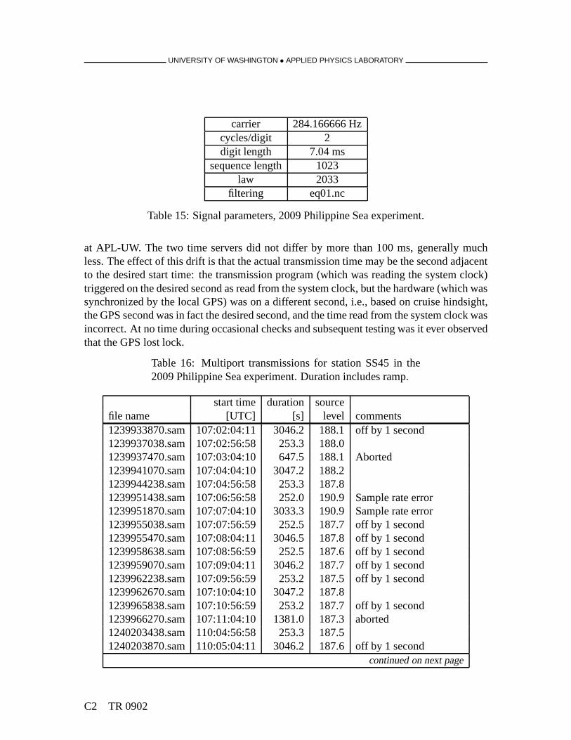
UNIVERSITY OF WASHINGTON • APPLIED PHYSICS LABORATORY
carrier 284.166666 Hzcycles/digit 2digit length 7.04 ms
sequence length 1023law 2033
filtering eq01.nc
Table 15: Signal parameters, 2009 Philippine Sea experiment.
at APL-UW. The two time servers did not differ by more than 100ms, generally muchless. The effect of this drift is that the actual transmission time may be the second adjacentto the desired start time: the transmission program (which was reading the system clock)triggered on the desired second as read from the system clock, but the hardware (which wassynchronized by the local GPS) was on a different second, i.e., based on cruise hindsight,the GPS second was in fact the desired second, and the time read from the system clock wasincorrect. At no time during occasional checks and subsequent testing was it ever observedthat the GPS lost lock.
Table 16: Multiport transmissions for station SS45 in the2009 Philippine Sea experiment. Duration includes ramp.
start time duration sourcefile name [UTC] [s] level comments1239933870.sam107:02:04:11 3046.2 188.1 off by 1 second1239937038.sam107:02:56:58 253.3 188.01239937470.sam107:03:04:10 647.5 188.1 Aborted1239941070.sam107:04:04:10 3047.2 188.21239944238.sam107:04:56:58 253.3 187.81239951438.sam107:06:56:58 252.0 190.9 Sample rate error1239951870.sam107:07:04:10 3033.3 190.9 Sample rate error1239955038.sam107:07:56:59 252.5 187.7 off by 1 second1239955470.sam107:08:04:11 3046.5 187.8 off by 1 second1239958638.sam107:08:56:59 252.5 187.6 off by 1 second1239959070.sam107:09:04:11 3046.2 187.7 off by 1 second1239962238.sam107:09:56:59 253.2 187.5 off by 1 second1239962670.sam107:10:04:10 3047.2 187.81239965838.sam107:10:56:59 253.2 187.7 off by 1 second1239966270.sam107:11:04:10 1381.0 187.3 aborted1240203438.sam110:04:56:58 253.3 187.51240203870.sam110:05:04:11 3046.2 187.6 off by 1 second
continued on next page
C2 TR 0902
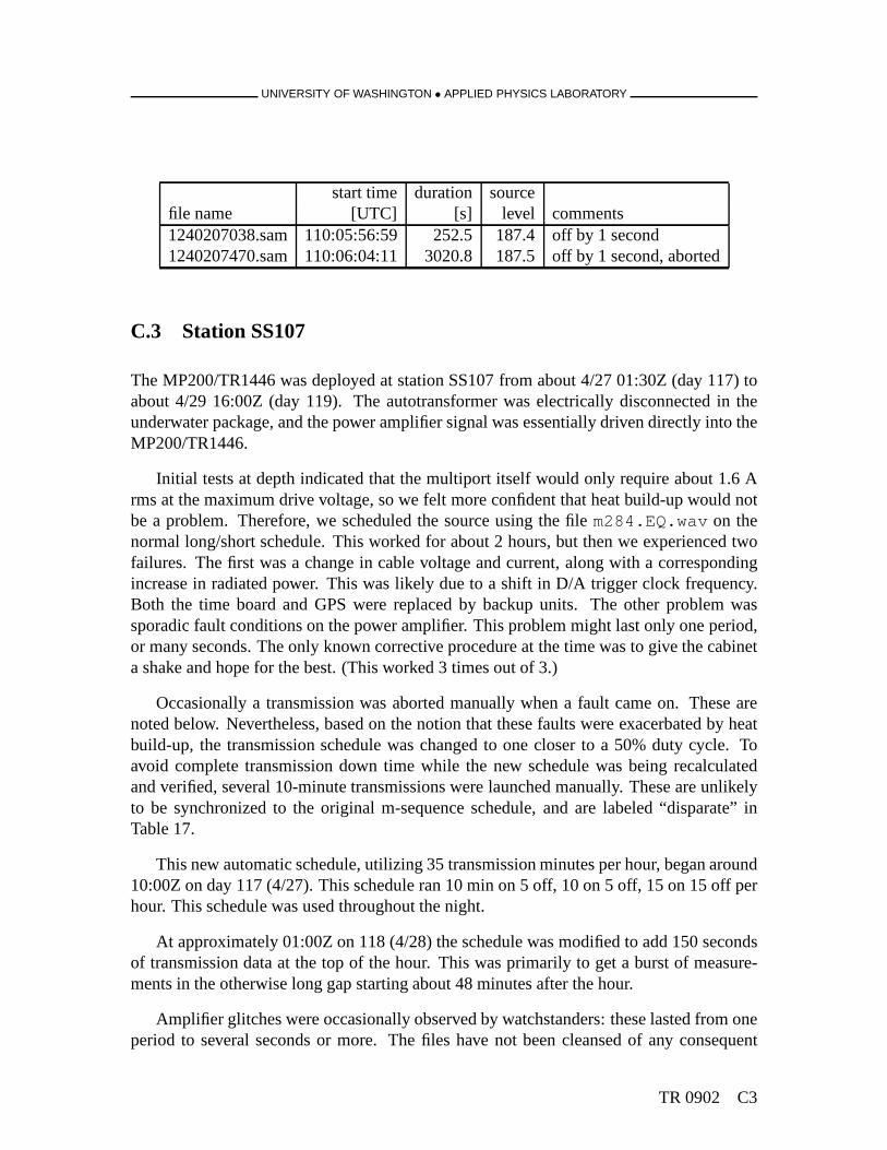
UNIVERSITY OF WASHINGTON • APPLIED PHYSICS LABORATORY
start time duration sourcefile name [UTC] [s] level comments1240207038.sam110:05:56:59 252.5 187.4 off by 1 second1240207470.sam110:06:04:11 3020.8 187.5 off by 1 second, aborted
C.3 Station SS107
The MP200/TR1446 was deployed at station SS107 from about 4/27 01:30Z (day 117) toabout 4/29 16:00Z (day 119). The autotransformer was electrically disconnected in theunderwater package, and the power amplifier signal was essentially driven directly into theMP200/TR1446.
Initial tests at depth indicated that the multiport itself would only require about 1.6 Arms at the maximum drive voltage, so we felt more confident that heat build-up would notbe a problem. Therefore, we scheduled the source using the file m284.EQ.wav on thenormal long/short schedule. This worked for about 2 hours, but then we experienced twofailures. The first was a change in cable voltage and current,along with a correspondingincrease in radiated power. This was likely due to a shift in D/A trigger clock frequency.Both the time board and GPS were replaced by backup units. Theother problem wassporadic fault conditions on the power amplifier. This problem might last only one period,or many seconds. The only known corrective procedure at the time was to give the cabineta shake and hope for the best. (This worked 3 times out of 3.)
Occasionally a transmission was aborted manually when a fault came on. These arenoted below. Nevertheless, based on the notion that these faults were exacerbated by heatbuild-up, the transmission schedule was changed to one closer to a 50% duty cycle. Toavoid complete transmission down time while the new schedule was being recalculatedand verified, several 10-minute transmissions were launched manually. These are unlikelyto be synchronized to the original m-sequence schedule, andare labeled “disparate” inTable 17.
This new automatic schedule, utilizing 35 transmission minutes per hour, began around10:00Z on day 117 (4/27). This schedule ran 10 min on 5 off, 10 on 5 off, 15 on 15 off perhour. This schedule was used throughout the night.
At approximately 01:00Z on 118 (4/28) the schedule was modified to add 150 secondsof transmission data at the top of the hour. This was primarily to get a burst of measure-ments in the otherwise long gap starting about 48 minutes after the hour.
Amplifier glitches were occasionally observed by watchstanders: these lasted from oneperiod to several seconds or more. The files have not been cleansed of any consequent
TR 0902 C3
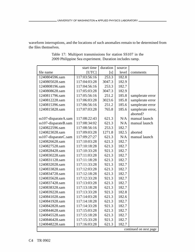
UNIVERSITY OF WASHINGTON • APPLIED PHYSICS LABORATORY
waveform interruptions, and the locations of such anomalies remain to be determined fromthe files themselves.
Table 17: Multiport transmissions for station SS107 in the2009 Philippine Sea experiment. Duration includes ramp.
start time duration sourcefile name [UTC] [s] level comments1240804596.sam 117:03:56:16 253.3 182.81240805028.sam 117:04:03:28 3047.3 182.91240808196.sam 117:04:56:16 253.3 182.71240808628.sam 117:05:03:28 3047.3 182.91240811796.sam 117:05:56:16 251.2 185.8 samplerate error1240812228.sam 117:06:03:28 3023.6 185.8 samplerate error1240815396.sam 117:06:56:16 251.2 185.6 samplerate error1240815828.sam 117:07:03:28 765.8 185.6 samplerate error,
aborted?ss107-disparateA.sam117:08:22:43 621.3 N/A manual launchss107-disparateB.sam117:08:34:02 621.3 N/A manual launch1240822596.sam 117:08:56:16 253.3 182.71240823028.sam 117:09:03:28 1271.8 182.5 abortedss107-disparateC.sam117:09:27:27 621.3 N/A manual launch1240826628.sam 117:10:03:28 621.3 182.71240827528.sam 117:10:18:28 621.3 182.71240828428.sam 117:10:33:28 921.3 182.71240830228.sam 117:11:03:28 621.3 182.71240831128.sam 117:11:18:28 621.3 182.71240832028.sam 117:11:33:28 921.3 182.71240833828.sam 117:12:03:28 621.3 182.71240834728.sam 117:12:18:28 621.3 182.71240835628.sam 117:12:33:28 921.3 182.71240837428.sam 117:13:03:28 621.3 182.71240838328.sam 117:13:18:28 621.3 182.71240839228.sam 117:13:33:28 921.3 182.81240841028.sam 117:14:03:28 621.3 182.61240841928.sam 117:14:18:28 621.3 182.71240842828.sam 117:14:33:28 921.3 182.71240844628.sam 117:15:03:28 621.3 182.71240845528.sam 117:15:18:28 621.3 182.71240846428.sam 117:15:33:28 921.3 182.71240848228.sam 117:16:03:28 621.3 182.7
continued on next page
C4 TR 0902

UNIVERSITY OF WASHINGTON • APPLIED PHYSICS LABORATORY
start time duration sourcefile name [UTC] [s] level comments1240849128.sam 117:16:18:28 621.3 182.71240850028.sam 117:16:33:28 921.3 182.71240851828.sam 117:17:03:28 621.3 182.61240852728.sam 117:17:18:28 621.3 182.61240853628.sam 117:17:33:28 921.3 182.61240855428.sam 117:18:03:28 621.3 182.61240856328.sam 117:18:18:28 621.3 182.61240857228.sam 117:18:33:28 921.3 182.61240859028.sam 117:19:03:28 621.3 182.61240859928.sam 117:19:18:28 621.3 182.61240860828.sam 117:19:33:28 921.3 182.71240862628.sam 117:20:03:28 621.3 182.81240863528.sam 117:20:18:28 621.3 182.71240864428.sam 117:20:33:28 921.3 182.71240866228.sam 117:21:03:28 621.3 182.71240867128.sam 117:21:18:28 621.3 182.71240868028.sam 117:21:33:28 921.3 182.81240869828.sam 117:22:03:28 621.3 182.61240870728.sam 117:22:18:28 621.3 182.51240871628.sam 117:22:33:28 921.3 182.51240873428.sam 117:23:03:28 621.3 182.51240874328.sam 117:23:18:28 621.3 182.61240875228.sam 117:23:33:28 921.3 182.61240877028.sam 118:00:03:28 621.3 182.51240877928.sam 118:00:18:28 621.3 182.51240878828.sam 118:00:33:28 921.3 182.61240880628.sam 118:01:03:28 621.3 182.61240881528.sam 118:01:18:28 621.3 182.61240882428.sam 118:01:33:28 921.3 182.61240883796.sam 118:01:56:16 171.3 182.21240884228.sam 118:02:03:28 621.3 182.51240885128.sam 118:02:18:28 921.3 182.51240886028.sam 118:02:33:28 621.3 182.61240887396.sam 118:02:56:16 171.3 182.31240887828.sam 118:03:03:28 921.3 182.41240888728.sam 118:03:18:28 621.3 182.61240889628.sam 118:03:33:28 621.3 182.61240890996.sam 118:03:56:16 171.3 182.2
continued on next page
TR 0902 C5
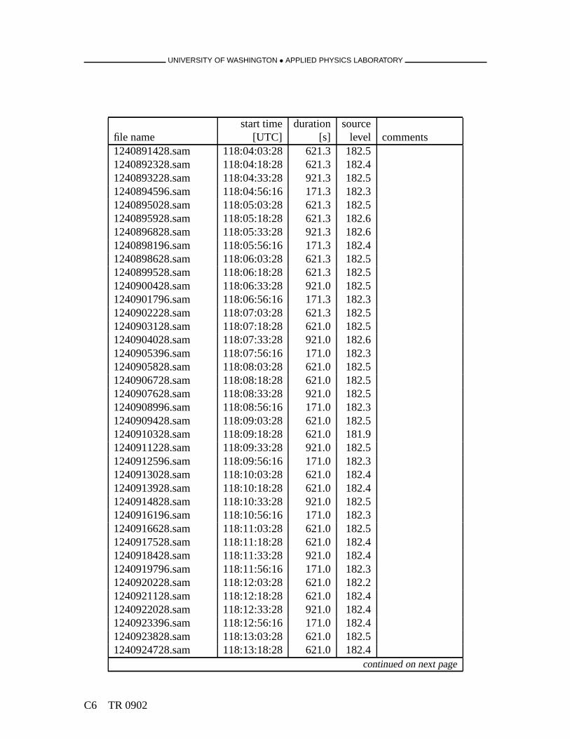
UNIVERSITY OF WASHINGTON • APPLIED PHYSICS LABORATORY
start time duration sourcefile name [UTC] [s] level comments1240891428.sam 118:04:03:28 621.3 182.51240892328.sam 118:04:18:28 621.3 182.41240893228.sam 118:04:33:28 921.3 182.51240894596.sam 118:04:56:16 171.3 182.31240895028.sam 118:05:03:28 621.3 182.51240895928.sam 118:05:18:28 621.3 182.61240896828.sam 118:05:33:28 921.3 182.61240898196.sam 118:05:56:16 171.3 182.41240898628.sam 118:06:03:28 621.3 182.51240899528.sam 118:06:18:28 621.3 182.51240900428.sam 118:06:33:28 921.0 182.51240901796.sam 118:06:56:16 171.3 182.31240902228.sam 118:07:03:28 621.3 182.51240903128.sam 118:07:18:28 621.0 182.51240904028.sam 118:07:33:28 921.0 182.61240905396.sam 118:07:56:16 171.0 182.31240905828.sam 118:08:03:28 621.0 182.51240906728.sam 118:08:18:28 621.0 182.51240907628.sam 118:08:33:28 921.0 182.51240908996.sam 118:08:56:16 171.0 182.31240909428.sam 118:09:03:28 621.0 182.51240910328.sam 118:09:18:28 621.0 181.91240911228.sam 118:09:33:28 921.0 182.51240912596.sam 118:09:56:16 171.0 182.31240913028.sam 118:10:03:28 621.0 182.41240913928.sam 118:10:18:28 621.0 182.41240914828.sam 118:10:33:28 921.0 182.51240916196.sam 118:10:56:16 171.0 182.31240916628.sam 118:11:03:28 621.0 182.51240917528.sam 118:11:18:28 621.0 182.41240918428.sam 118:11:33:28 921.0 182.41240919796.sam 118:11:56:16 171.0 182.31240920228.sam 118:12:03:28 621.0 182.21240921128.sam 118:12:18:28 621.0 182.41240922028.sam 118:12:33:28 921.0 182.41240923396.sam 118:12:56:16 171.0 182.41240923828.sam 118:13:03:28 621.0 182.51240924728.sam 118:13:18:28 621.0 182.4
continued on next page
C6 TR 0902
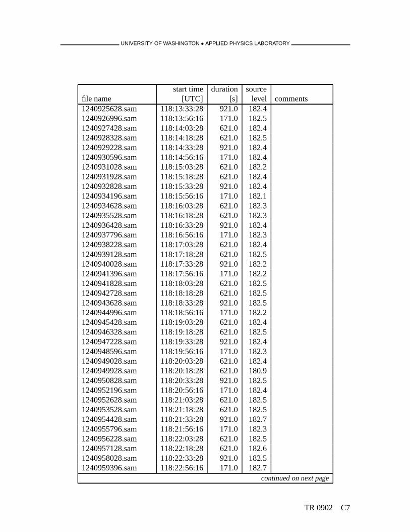
UNIVERSITY OF WASHINGTON • APPLIED PHYSICS LABORATORY
start time duration sourcefile name [UTC] [s] level comments1240925628.sam 118:13:33:28 921.0 182.41240926996.sam 118:13:56:16 171.0 182.51240927428.sam 118:14:03:28 621.0 182.41240928328.sam 118:14:18:28 621.0 182.51240929228.sam 118:14:33:28 921.0 182.41240930596.sam 118:14:56:16 171.0 182.41240931028.sam 118:15:03:28 621.0 182.21240931928.sam 118:15:18:28 621.0 182.41240932828.sam 118:15:33:28 921.0 182.41240934196.sam 118:15:56:16 171.0 182.11240934628.sam 118:16:03:28 621.0 182.31240935528.sam 118:16:18:28 621.0 182.31240936428.sam 118:16:33:28 921.0 182.41240937796.sam 118:16:56:16 171.0 182.31240938228.sam 118:17:03:28 621.0 182.41240939128.sam 118:17:18:28 621.0 182.51240940028.sam 118:17:33:28 921.0 182.21240941396.sam 118:17:56:16 171.0 182.21240941828.sam 118:18:03:28 621.0 182.51240942728.sam 118:18:18:28 621.0 182.51240943628.sam 118:18:33:28 921.0 182.51240944996.sam 118:18:56:16 171.0 182.21240945428.sam 118:19:03:28 621.0 182.41240946328.sam 118:19:18:28 621.0 182.51240947228.sam 118:19:33:28 921.0 182.41240948596.sam 118:19:56:16 171.0 182.31240949028.sam 118:20:03:28 621.0 182.41240949928.sam 118:20:18:28 621.0 180.91240950828.sam 118:20:33:28 921.0 182.51240952196.sam 118:20:56:16 171.0 182.41240952628.sam 118:21:03:28 621.0 182.51240953528.sam 118:21:18:28 621.0 182.51240954428.sam 118:21:33:28 921.0 182.71240955796.sam 118:21:56:16 171.0 182.31240956228.sam 118:22:03:28 621.0 182.51240957128.sam 118:22:18:28 621.0 182.61240958028.sam 118:22:33:28 921.0 182.51240959396.sam 118:22:56:16 171.0 182.7
continued on next page
TR 0902 C7

UNIVERSITY OF WASHINGTON • APPLIED PHYSICS LABORATORY
start time duration sourcefile name [UTC] [s] level comments1240959828.sam 118:23:03:28 621.0 182.51240960728.sam 118:23:18:28 621.0 182.41240961628.sam 118:23:33:28 921.0 182.41240962996.sam 118:23:56:16 171.0 182.31240963428.sam 119:00:03:28 621.0 182.41240964328.sam 119:00:18:28 621.0 182.51240965228.sam 119:00:33:28 921.0 182.51240966596.sam 119:00:56:16 171.0 182.41240967028.sam 119:01:03:28 621.0 182.51240967928.sam 119:01:18:28 621.0 181.71240968828.sam 119:01:33:28 921.0 182.41240970628.sam 119:02:03:28 621.0 182.41240971528.sam 119:02:18:28 241.0 181.7 Aborted1240972428.sam 119:02:33:28 921.0 182.41240973796.sam 119:02:56:16 171.0 182.31240974228.sam 119:03:03:28 621.0 182.51240975128.sam 119:03:18:28 621.0 182.41240976028.sam 119:03:33:28 921.0 182.51240977396.sam 119:03:56:16 171.0 182.21240977828.sam 119:04:03:28 621.0 182.81240978728.sam 119:04:18:28 621.0 182.41240979628.sam 119:04:33:28 921.0 182.41240980996.sam 119:04:56:16 171.0 182.21240981428.sam 119:05:03:28 621.0 182.21240982328.sam 119:05:18:28 621.0 182.21240983228.sam 119:05:33:28 921.0 182.41240984596.sam 119:05:56:16 171.0 182.21240985028.sam 119:06:03:28 621.0 185.71240985928.sam 119:06:18:28 621.0 183.01240986828.sam 119:06:33:28 921.0 187.91240988196.sam 119:06:56:16 171.0 182.41240988628.sam 119:07:03:28 621.0 182.21240989528.sam 119:07:18:28 621.0 182.21240990428.sam 119:07:33:28 921.0 182.41240991796.sam 119:07:56:16 171.0 182.11240992228.sam 119:08:03:28 621.0 182.31240993128.sam 119:08:18:28 621.0 182.41240994028.sam 119:08:33:28 921.0 182.3
continued on next page
C8 TR 0902
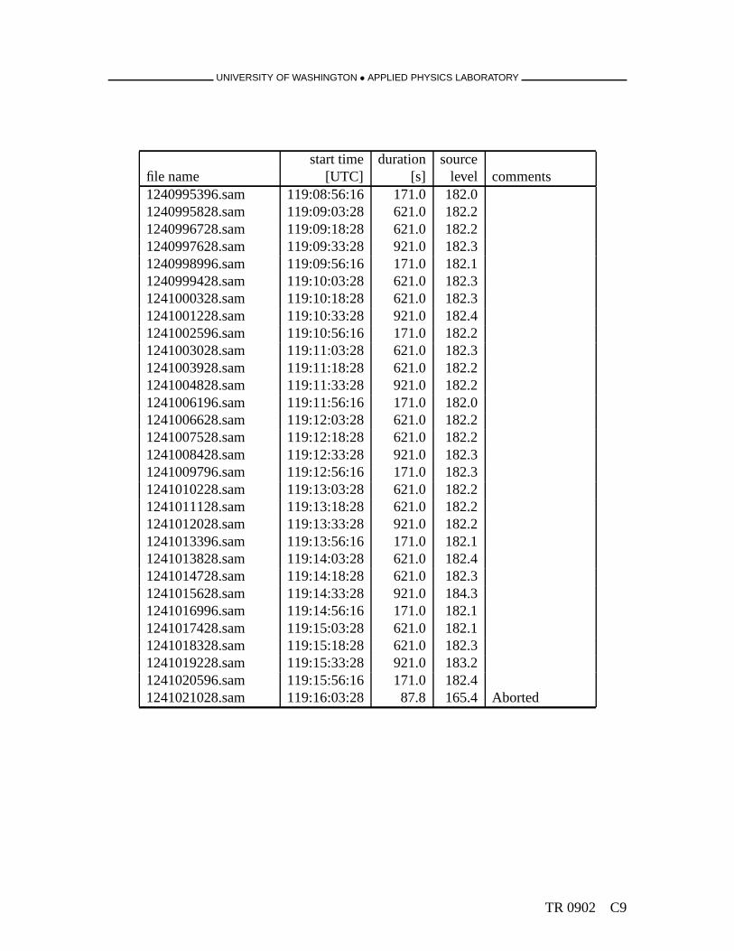
UNIVERSITY OF WASHINGTON • APPLIED PHYSICS LABORATORY
start time duration sourcefile name [UTC] [s] level comments1240995396.sam 119:08:56:16 171.0 182.01240995828.sam 119:09:03:28 621.0 182.21240996728.sam 119:09:18:28 621.0 182.21240997628.sam 119:09:33:28 921.0 182.31240998996.sam 119:09:56:16 171.0 182.11240999428.sam 119:10:03:28 621.0 182.31241000328.sam 119:10:18:28 621.0 182.31241001228.sam 119:10:33:28 921.0 182.41241002596.sam 119:10:56:16 171.0 182.21241003028.sam 119:11:03:28 621.0 182.31241003928.sam 119:11:18:28 621.0 182.21241004828.sam 119:11:33:28 921.0 182.21241006196.sam 119:11:56:16 171.0 182.01241006628.sam 119:12:03:28 621.0 182.21241007528.sam 119:12:18:28 621.0 182.21241008428.sam 119:12:33:28 921.0 182.31241009796.sam 119:12:56:16 171.0 182.31241010228.sam 119:13:03:28 621.0 182.21241011128.sam 119:13:18:28 621.0 182.21241012028.sam 119:13:33:28 921.0 182.21241013396.sam 119:13:56:16 171.0 182.11241013828.sam 119:14:03:28 621.0 182.41241014728.sam 119:14:18:28 621.0 182.31241015628.sam 119:14:33:28 921.0 184.31241016996.sam 119:14:56:16 171.0 182.11241017428.sam 119:15:03:28 621.0 182.11241018328.sam 119:15:18:28 621.0 182.31241019228.sam 119:15:33:28 921.0 183.21241020596.sam 119:15:56:16 171.0 182.41241021028.sam 119:16:03:28 87.8 165.4 Aborted
TR 0902 C9
REPORT DOCUMENTATION PAGEForm Approved
OPM No. 0704-0188
Public reporting burden for this collection of information is estimated to average 1 hour per response, including the time for reviewing instructions, searching existing data sources, gathering and maintaining the data needed, and reviewing the collection of information. Send comments regarding this burden estimate or any other aspect of this collection of information, including suggestions for reducing this burden, to Washington Headquarters Services, Directorate for Information Operations and Reports, 1215 Jefferson Davis Highway, Suite 1204, Arlington, VA 22202-4302, and to the Office of Information and Regulatory Affairs, Office of Management and Budget, Washington, DC 20503.
1. AGENCY USE ONLY 2. REPORT DATE 3. REPORT TYPE AND DATES COVERED
5. FUNDING NUMBERS4. TITLE AND SUBTITLE
6. AUTHOR(S)
7. PERFORMING ORGANIZATION NAME(S) AND ADDRESS(ES) 8. PERFORMING ORGANIZATION REPORT NUMBER
9. SPONSORING / MONITORING AGENCY NAME(S) AND ADDRESS(ES) 10. SPONSORING / MONITORING AGENCY REPORT NUMBER
11. SUPPLEMENTARY NOTES
12a. DISTRIBUTION / AVAILABILITY STATEMENT12a. DISTRIBUTION / AVAILABILITY STATEMENT 12b. DISTRIBUTION CODE
13. ABSTRACT (Maximum 200 words)
14. SUBJECT TERMS
17. SECURITY CLASSIFICATION OF REPORT
18. SECURITY CLASSIFICATION OF THIS PAGE
19. SECURITY CLASSIFICATION OF ABSTRACT
15. NUMBER OF PAGES
16. PRICE CODE
20. LIMITATION OF ABSTRACT
NSN 7540-01-280-5500 Standard Form 298 (Rev. 2-89)Prescribed by ANSI Std. 239-18299-01
N00014-03-1-0181,N00014-07-1-0743,N00014-08-1-0843
December 2009 Technical Report
Dr. Ellen LivingstonOffice of Naval Research, Code 321OAOne Liberty Center875 North Randolph Street Suite 1425Arlington, VA 22203-1995
Rex K. Andrew
Unclassified Unclassified Unclassified SAR
102Underwater acoustic transducer, Multiport source, Signal equalization, Ocean acoustic tomography, PhilSea09
The Applied Physics Laboratory of the University of Washington (APL-UW) has acquired on loan an experimental device known as the multiport transducer. APL-UW has developed, in turn, a complete transmitter system that integrated this trans-ducer, capable of wideband operation (roughly 180–350 Hz) from near-surface depths to depths greater than 1000 m. The system's electrical components include an autotransformer tuner, a sea battery, and a fibre optic telemetry interface; mechanical components include a steel supporting structure and a pressure-compensated tuner housing; an additional acoustical component is a monitor hydrophone in a vibration isolation mount; and a signal component involves a lumped parameter SPICE circuit model approximation of the entire end-to-end system, an associated C++ application to predict the time-domain acoustic far field from a standard time-domain waveform input file, and a pre-equalization filter. The multiport system was a key element in a 2009 at-sea acoustics experiment located in the Philippine Sea and provided many hours of high-quality pulsed transmissions to a nearby vertical line array of hydrophones.
The APL-UW Multiport Acoustic Projector System
Approved for public release; distribution is unlimited.
Applied Physics LaboratoryUniversity of Washington1013 NE 40th StreetSeattle, WA 98105-6698