the 1925 born and jordan paper “on quantum mechanics” · pdf filethe 1925 born and...

The 1925 Born and Jordan paper “On quantum mechanics”William A. Fedaka� and Jeffrey J. Prentisb�

Department of Natural Sciences, University of Michigan–Dearborn, Dearborn, Michigan 48128

�Received 12 September 2007; accepted 9 October 2008�

The 1925 paper “On quantum mechanics” by M. Born and P. Jordan, and the sequel “On quantummechanics II” by M. Born, W. Heisenberg, and P. Jordan, developed Heisenberg’s pioneering theoryinto the first complete formulation of quantum mechanics. The Born and Jordan paper is the subjectof the present article. This paper introduced matrices to physicists. We discuss the original postulatesof quantum mechanics, present the two-part discovery of the law of commutation, and clarify theorigin of Heisenberg’s equation. We show how the 1925 proof of energy conservation and Bohr’sfrequency condition served as the gold standard with which to measure the validity of the newquantum mechanics. © 2009 American Association of Physics Teachers.

�DOI: 10.1119/1.3009634�

I. INTRODUCTION

The name “quantum mechanics” was coined by MaxBorn.1 For Born and others, quantum mechanics denoted acanonical theory of atomic and electronic motion of the samelevel of generality and consistency as classical mechanics.The transition from classical mechanics to a true quantummechanics remained an elusive goal prior to 1925.

Heisenberg made the breakthrough in his historic 1925paper, “Quantum-theoretical reinterpretation of kinematicand mechanical relations.”2 Heisenberg’s bold idea was toretain the classical equations of Newton but to replace theclassical position coordinate with a “quantum-theoreticalquantity.” The new position quantity contains informationabout the measurable line spectrum of an atom rather thanthe unobservable orbit of the electron. Born realized thatHeisenberg’s kinematical rule for multiplying position quan-tities was equivalent to the mathematical rule for multiplyingmatrices. The next step was to formalize Heisenberg’s theoryusing the language of matrices.

The first comprehensive exposition on quantum mechanicsin matrix form was written by Born and Jordan,4 and thesequel was written by Born, Heisenberg, and Jordan.5 Diracindependently discovered the general equations of quantummechanics without using matrix theory.6 These papers devel-oped a Hamiltonian mechanics of the atom in a completelynew quantum �noncommutative� format. These papers ush-ered in a new era in theoretical physics where Hermitianmatrices, commutators, and eigenvalue problems became themathematical trademark of the atomic world. We discuss thefirst paper “On quantum mechanics.”4

This formulation of quantum mechanics, now referred toas matrix mechanics,7 marked one of the most intense peri-ods of discovery in physics. The ideas and formalism behindthe original matrix mechanics are absent in most textbooks.Recent articles discuss the correspondence between classicalharmonics and quantum jumps,8 the calculational details ofHeisenberg’s paper,9 and the role of Born in the creation ofquantum theory.10 References 11–19 represent a sampling ofthe many sources on the development of quantum mechan-ics.

Given Born and Jordan’s pivotal role in the discovery ofquantum mechanics, it is natural to wonder why there are noequations named after them,20 and why they did not share theNobel Prize with others.21 In 1933 Heisenberg wrote Born
saying “The fact that I am to receive the Nobel Prize alone,
128 Am. J. Phys. 77 �2�, February 2009 http://aapt.org/ajp

for work done in Göttingen in collaboration—you, Jordan,and I, this fact depresses me and I hardly know what to writeto you. I am, of course, glad that our common efforts arenow appreciated, and I enjoy the recollection of the beautifultime of collaboration. I also believe that all good physicistsknow how great was your and Jordan’s contribution to thestructure of quantum mechanics—and this remains un-changed by a wrong decision from outside. Yet I myself cando nothing but thank you again for all the fine collaborationand feel a little ashamed.”23

Engraved on Max Born’s tombstone is a one-line epitaph:pq−qp=h /2�i. Born composed this elegant equation inearly July 1925 and called it “die verschärfteQuantenbedingung”4—the sharpened quantum condition.This equation is now known as the law of commutation andis the hallmark of quantum algebra.

In the contemporary approach to teaching quantum me-chanics, matrix mechanics is usually introduced after a thor-ough discussion of wave mechanics. The Heisenberg pictureis viewed as a unitary transformation of the Schrödingerpicture.24 How was matrix mechanics formulated in 1925when the Schrödinger picture was nowhere in sight? TheBorn and Jordan paper4 represents matrix mechanics in itspurest form.

II. BACKGROUND TO “ON QUANTUMMECHANICS”

Heisenberg’s program, as indicated by the title of hispaper,2 consisted of constructing quantum-theoretical rela-tions by reinterpreting the classical relations. To appreciatewhat Born and Jordan did with Heisenberg’s reinterpreta-tions, we discuss in the Appendix four key relations fromHeisenberg’s paper.2 Heisenberg wrote the classical andquantum versions of each relation in parallel—as formulacouplets. Heisenberg has been likened to an “expert decoderwho reads a cryptogram.”25 The correspondence principle8,26

acted as a “code book” for translating a classical relation intoits quantum counterpart. Unlike his predecessors who usedthe correspondence principle to produce specific relations,Heisenberg produced an entirely new theory—complete witha new representation of position and a new rule of multipli-cation, together with an equation of motion and a quantumcondition whose solution determined the atomic observables
�energies, frequencies, and transition amplitudes�.
128© 2009 American Association of Physics Teachers

Matrices are not explicitly mentioned in Heisenberg’s pa-per. He did not arrange his quantum-theoretical quantitiesinto a table or array. In looking back on his discovery,Heisenberg wrote, “At that time I must confess I did notknow what a matrix was and did not know the rules of ma-trix multiplication.”18 In the last sentence of his paper hewrote “whether this method after all represents far too roughan approach to the physical program of constructing a theo-retical quantum mechanics, an obviously very involved prob-lem at the moment, can be decided only by a more intensivemathematical investigation of the method which has beenvery superficially employed here.”27

Born took up Heisenberg’s challenge to pursue “a moreintensive mathematical investigation.” At the time Heisen-berg wrote his paper, he was Born’s assistant at the Univer-sity of Göttingen. Born recalls the moment of inspirationwhen he realized that position and momentum werematrices:28

After having sent Heisenberg’s paper to theZeitschrift für Physik for publication, I began toponder about his symbolic multiplication, and wassoon so involved in it…For I felt there was some-thing fundamental behind it…And one morning,about 10 July 1925, I suddenly saw the light:Heisenberg’s symbolic multiplication was nothingbut the matrix calculus, well known to me sincemy student days from the lectures of Rosanes inBreslau.

I found this by just simplifying the notation a little:instead of q�n ,n+��, where n is the quantum num-ber of one state and � the integer indicating thetransition, I wrote q�n ,m�, and rewriting Heisen-berg’s form of Bohr’s quantum condition, I recog-nized at once its formal significance. It meant thatthe two matrix products pq and qp are not identi-cal. I was familiar with the fact that matrix multi-plication is not commutative; therefore I was nottoo much puzzled by this result. Closer inspectionshowed that Heisenberg’s formula gave only thevalue of the diagonal elements �m=n� of the ma-trix pq–qp; it said they were all equal and had thevalue h /2�i where h is Planck’s constant and i=�−1. But what were the other elements �m�n�?

Here my own constructive work began. RepeatingHeisenberg’s calculation in matrix notation, I soonconvinced myself that the only reasonable value ofthe nondiagonal elements should be zero, and Iwrote the strange equation

pq − qp =h

2�i1 , �1�

where 1 is the unit matrix. But this was only aguess, and all my attempts to prove it failed.

On 19 July 1925, Born invited his former assistant Wolf-

129 Am. J. Phys., Vol. 77, No. 2, February 2009

gang Pauli to collaborate on the matrix program. Pauli de-clined the invitation.29 The next day, Born asked his studentPascual Jordan to assist him. Jordan accepted the invitationand in a few days proved Born’s conjecture that all nondi-agonal elements of pq−qp must vanish. The rest of the newquantum mechanics rapidly solidified. The Born and Jordanpaper was received by the Zeitschrift für Physik on 27 Sep-tember 1925, two months after Heisenberg’s paper was re-ceived by the same journal. All the essentials of matrix me-chanics as we know the subject today fill the pages of thispaper.

In the abstract Born and Jordan wrote “The recently pub-lished theoretical approach of Heisenberg is here developedinto a systematic theory of quantum mechanics �in the firstplace for systems having one degree of freedom� with the aidof mathematical matrix methods.”30 In the introduction theygo on to write “The physical reasoning which led Heisenbergto this development has been so clearly described by himthat any supplementary remarks appear superfluous. But, ashe himself indicates, in its formal, mathematical aspects hisapproach is but in its initial stages. His hypotheses have beenapplied only to simple examples without being fully carriedthrough to a generalized theory. Having been in an advanta-geous position to familiarize ourselves with his ideasthroughout their formative stages, we now strive �since hisinvestigations have been concluded� to clarify the math-ematically formal content of his approach and present someof our results here. These indicate that it is in fact possible,starting with the basic premises given by Heisenberg, tobuild up a closed mathematical theory of quantum mechanicswhich displays strikingly close analogies with classical me-chanics, but at the same time preserves the characteristicfeatures of quantum phenomena.”31

The reader is introduced to the notion of a matrix in thethird paragraph of the introduction: “The mathematical basisof Heisenberg’s treatment is the law of multiplication ofquantum-theoretical quantities, which he derived from an in-genious consideration of correspondence arguments. The de-velopment of his formalism, which we give here, is basedupon the fact that this rule of multiplication is none otherthan the well-known mathematical rule of matrix multiplica-tion. The infinite square array which appears at the start ofthe next section, termed a matrix, is a representation of aphysical quantity which is given in classical theory as a func-tion of time. The mathematical method of treatment inherentin the new quantum mechanics is thereby characterized bythe employment of matrix analysis in place of the usualnumber analysis.”

The Born-Jordan paper4 is divided into four chapters.Chapter 1 on “Matrix calculation” introduces the mathemat-ics �algebra and calculus� of matrices to physicists. Chapter 2on “Dynamics” establishes the fundamental postulates ofquantum mechanics, such as the law of commutation, andderives the important theorems, such as the conservation ofenergy. Chapter 3 on “Investigation of the anharmonic oscil-lator” contains the first rigorous �correspondence free� calcu-lation of the energy spectrum of a quantum-mechanical har-monic oscillator. Chapter 4 on “Remarks onelectrodynamics” contains a procedure—the first of itskind—to quantize the electromagnetic field. We focus on thematerial in Chap. 2 because it contains the essential physics
of matrix mechanics.
129William A. Fedak and Jeffrey J. Prentis

III. THE ORIGINAL POSTULATES OF QUANTUMMECHANICS

Current presentations of quantum mechanics frequentlyare based on a set of postulates.32 The Born–Jordan postu-lates of quantum mechanics were crafted before wave me-chanics was formulated and thus are quite different than theSchrödinger-based postulates in current textbooks. The origi-nal postulates come as close as possible to the classical-mechanical laws while maintaining complete quantum-mechanical integrity.

Section III, “The basic laws,” in Chap. 2 of the Born–Jordan paper is five pages long and contains approximatelythirty equations. We have imposed a contemporary postula-tory approach on this section by identifying five fundamentalpassages from the text. We call these five fundamental ideas“the postulates.” We have preserved the original phrasing,notation, and logic of Born and Jordan. The labeling and thenaming of the postulates is ours.

Postulate 1. Position and Momentum. Born and Jordanintroduce the position and momentum matrices by writingthat33

The dynamical system is to be described by thespatial coordinate q and the momentum p, thesebeing represented by the matrices

�q = q�nm�e2�i��nm�t� ,

�p = p�nm�e2�i��nm�t� . �2�

Here the ��nm� denote the quantum-theoretical fre-quencies associated with the transitions betweenstates described by the quantum numbers n and m.The matrices �2� are to be Hermitian, e.g., on trans-position of the matrices, each element is to go overinto its complex conjugate value, a conditionwhich should apply for all real t. We thus have

q�nm�q�mn� = �q�nm��2 �3�

and

��nm� = − ��mn� . �4�

If q is a Cartesian coordinate, then the expression�3� is a measure of the probabilities of the transi-tions n�m.

The preceding passage placed Hermitian matrices into thephysics limelight. Prior to the Born–Jordan paper, matriceswere rarely seen in physics.34 Hermitian matrices were evenstranger. Physicists were reluctant to accept such an abstractmathematical entity as a description of physical reality.

For Born and Jordan, q and p do not specify the positionand momentum of an electron in an atom. Heisenbergstressed that quantum theory should focus only on the ob-servable properties, namely the frequency and intensity ofthe atomic radiation and not the position and period of theelectron. The quantities q and p represent position and mo-mentum in the sense that q and p satisfy matrix equations of
motion that are identical in form to those satisfied by the

position and momentum of classical mechanics. In the Bohratom the electron undergoes periodic motion in a well de-fined orbit around the nucleus with a certain classical fre-quency. In the Heisenberg–Born–Jordan atom there is nolonger an orbit, but there is some sort of periodic “quantummotion” of the electron characterized by the set of frequen-cies ��nm� and amplitudes q�nm�. Physicists believed thatsomething inside the atom must vibrate with the right fre-quencies even though they could not visualize what thequantum oscillations looked like. The mechanical properties�q ,p� of the quantum motion contain complete informationon the spectral properties �frequency, intensity� of the emit-ted radiation.

The diagonal elements of a matrix correspond to thestates, and the off-diagonal elements correspond to the tran-sitions. An important property of all dynamical matrices isthat the diagonal elements are independent of time. The Her-mitian rule in Eq. �4� implies the relation ��nn�=0. Thus thetime factor of the nth diagonal term in any matrix ise2�i��nn�t=1. As we shall see, the time-independent entries ina diagonal matrix are related to the constant values of a con-served quantity.

In their purely mathematical introduction to matrices�Chap. 1�, Born and Jordan use the following symbols todenote a matrix

a = �a�nm�� =�a�00� a�01� a�02� . . .

a�10� a�11� a�12�a�20� a�21� a�22�] �

� . �5�

The bracketed symbol �a�nm��, which displays inner ele-ments a�nm� contained within outer brackets � �, is the short-hand notation for the array in Eq. �5�. By writing the matrixelements as a�nm�, rather than anm, Born and Jordan madedirect contact with Heisenberg’s quantum-theoretical quanti-ties a�n ,n−�� see the Appendix�. They wrote35 “Matrixmultiplication is defined by the rule ‘rows times columns,’familiar from the ordinary theory of determinants:

a = bc means a�nm� = k=0

�

b�nk�c�km� . ” �6�

This multiplication rule was first given �for finite square ma-trices� by Arthur Cayley.36 Little did Cayley know in 1855that his mathematical “row times column” expressionb�nk�c�km� would describe the physical process of an elec-tron making the transition n→k→m in an atom.

Born and Jordan wrote in Postulate 1 that the quantity�q�nm��2 provides “a measure of the probabilities of the tran-sitions n�m.” They justify this profound claim in the lastchapter.37 Born and Jordan’s one-line claim about transitionprobabilities is the only statistical statement in their postu-lates. Physics would have to wait several months beforeSchrödinger’s wave function ��x� and Born’s probabilityfunction ��x��2 entered the scene. Born discovered the con-nection between ��x��2 and position probability, and wasalso the first physicist �with Jordan� to formalize the connec-tion between �q�nm��2 and the transition probability via a“quantum electrodynamic” argument.38 As a pioneer statisti-cal interpreter of quantum mechanics, it is interesting to
speculate that Born might have discovered how to form a

�

linear superposition of the periodic matrix elementsq�nm�e2�i��nm�t in order to obtain another statistical object,namely the expectation value q�. Early on, Born, Heisen-berg, and Jordan did superimpose matrix elements,47 but didnot supply the statistical interpretation.

Postulate 2. Frequency Combination Principle. After de-fining q and p, Born and Jordan wrote39 “Further, we shallrequire that

��jk� + ��kl� + ��lj� = 0 . ” �7�

The frequency sum rule in Eq. �7� is the fundamental con-straint on the quantum-theoretical frequencies. This rule isbased on the Ritz combination principle, which explains therelations of the spectral lines of atomic spectroscopy.40 Equa-tion �7� is the quantum analogue of the “Fourier combinationprinciple”, ��k− j�+��l−k�+��j− l�=0, where ��=��1�is the frequency of the �th harmonic component of a Fourierseries. The frequency spectrum of classical periodic motionobeys this Fourier sum rule. The equal Fourier spacing ofclassical lines is replaced by the irregular Ritzian spacing ofquantal lines. In the correspondence limit of large quantumnumbers and small quantum jumps the atomic spectrum ofRitz reduces to the harmonic spectrum of Fourier.8,26 Be-cause the Ritz rule was considered an exact law of atomicspectroscopy, and because Fourier series played a vital rolein Heisenberg’s analysis, it made sense for Born and Jordanto posit the frequency rule in Eq. �7� as a basic law.

One might be tempted to regard Eq. �7� as equivalent tothe Bohr frequency condition, E�n�−E�m�=h��nm�, whereE�n� is the energy of the stationary state n. For Born andJordan, Eq. �7� says nothing about energy. They note thatEqs. �4� and �7� imply that there exists spectral terms Wnsuch that

h��nm� = Wn − Wm. �8�

At this postulatory stage, the term Wn of the spectrum isunrelated to the energy E�n� of the state. Heisenberg empha-sized this distinction between “term” and “energy” in a letterto Pauli summarizing the Born–Jordan theory.41 Born andJordan adopt Eq. �7� as a postulate–one based solely on theobservable spectral quantities ��nm� without reference to anymechanical quantities E�n�. The Bohr frequency condition isnot something they assume a priori, it is something that mustbe rigorously proved.

The Ritz rule insures that the nm element of any dynami-cal matrix �any function of p and q� oscillates with the samefrequency ��nm� as the nm element of p and q. For example,if the 3→2 elements of p and q oscillate at 500 MHz, thenthe 3→2 elements of p2, q2, pq, q3, p2+q2, etc. each oscil-late at 500 MHz. In all calculations involving the canonicalmatrices p and q, no new frequencies are generated. A con-sistent quantum theory must preserve the frequency spectrumof a particular atom because the spectrum is the spectro-scopic signature of the atom. The calculations must notchange the identity of the atom. Based on the rules for ma-nipulating matrices and combining frequencies, Born andJordan wrote that “it follows that a function g�pq� invariablytakes on the form

g = �g�nm�e2�i��nm�t� �9�

and the matrix �g�nm�� therein results from identically the
same process applied to the matrices �q�nm��, �p�nm�� as

was employed to find g from q, p.”42 Because e2�i��nm�t is theuniversal time factor common to all dynamical matrices, theynote that it can be dropped from Eq. �2� in favor of theshorter notation q= �q�nm�� and p= �p�nm��.

Why does the Ritz rule insure that the time factors ofg�pq� are identical to the time factors of p and q? Considerthe potential energy function q2. The nm element of q2,which we denote by q2�nm�, is obtained from the elements ofq via the multiplication rule

q2�nm� = k

q�nk�e2�i��nk�tq�km�e2�i��km�t. �10�

Given the Ritz relation ��nm�=��nk�+��km�, which followsfrom Eqs. �4� and �7�, Eq. �10� reduces to

q2�nm� = �k

q�nk�q�km� e2�i��nm�t. �11�

It follows that the nm time factor of q2 is the same as the nmtime factor of q.

We see that the theoretical rule for multiplying mechanicalamplitudes, a�nm�=kb�nk�c�km�, is intimately related tothe experimental rule for adding spectral frequencies,��nm�=��nk�+��km�. The Ritz rule occupied a prominentplace in Heisenberg’s discovery of the multiplication rule�see the Appendix�. Whenever a contemporary physicist cal-culates the total amplitude of the quantum jump n→k→m,the steps involved can be traced back to the frequency com-bination principle of Ritz.

Postulate 3. The Equation of Motion. Born and Jordanintroduce the law of quantum dynamics by writing43

In the case of a Hamilton function having the form

H =1

2mp2 + U�q� , �12�

we shall assume, as did Heisenberg, that the equa-tions of motion have just the same form as in theclassical theory, so that we can write:

q =�H

�p=

1

mp , �13a�

p = −�H

�q= −

�U

�q. �13b

This Hamiltonian formulation of quantum dynamics general-ized Heisenberg’s Newtonian approach.44 The assumption byHeisenberg and Born and Jordan that quantum dynamicslooks the same as classical dynamics was a bold and deepassumption. For them, the problem with classical mechanicswas not the dynamics �the form of the equations of motion�,but rather the kinematics �the meaning of position and mo-mentum�.

Postulate 4. Energy Spectrum. Born and Jordan reveal theconnection between the allowed energies of a conservativesystem and the numbers in the Hamiltonian matrix:

“The diagonal elements H�nn� of H are inter-preted, according to Heisenberg, as the energies of

45
the various states of the system.”

This statement introduced a radical new idea into main-stream physics: calculating an energy spectrum reduces tofinding the components of a diagonal matrix.46 AlthoughBorn and Jordan did not mention the word eigenvalue in Ref.4, Born, Heisenberg, and Jordan would soon formalize theidea of calculating an energy spectrum by solving an eigen-value problem.5 The ad hoc rules for calculating a quantizedenergy in the old quantum theory were replaced by a system-atic mathematical program.

Born and Jordan considered exclusively conservative sys-tems for which H does not depend explicitly on time. Theconnection between conserved quantities and diagonal matri-ces will be discussed later. For now, recall that the diagonalelements of any matrix are independent of time. For the spe-cial case where all the non-diagonal elements of a dynamicalmatrix g�pq� vanish, the quantity g is a constant of the mo-tion. A postulate must be introduced to specify the physicalmeaning of the constant elements in g.

In the old quantum theory it was difficult to explain whythe energy was quantized. The discontinuity in energy had tobe postulated or artificially imposed. Matrices are naturallyquantized. The quantization of energy is built into the dis-crete row-column structure of the matrix array. In the oldtheory Bohr’s concept of a stationary state of energy En wasa central concept. Physicists grappled with the questions:Where does En fit into the theory? How is En calculated?Bohr’s concept of the energy of the stationary state finallyfound a rigorous place in the new matrix scheme.47

Postulate 5. The Quantum Condition. Born and Jordanstate that the elements of p and q for any quantum mechani-cal system must satisfy the “quantum condition”:

k

�p�nk�q�kn� − q�nk�p�kn�� =h

2�i. �14�

Given the significance of Eq. �14� in the development ofquantum mechanics, we quote Born and Jordan’s “deriva-tion” of this equation:

The equation

J = � pdq = �0

1/�

pqdt �15�

of “classical” quantum theory can, on introducingthe Fourier expansions of p and q,

p = �=−�

�

p�e2�i��t,

�16�

q = �=−�

�

q�e2�i��t,

be transformed into

1 = 2�i �=−�

�

��

�J�q�p−�� . �17�

The following expressions should correspond:


�=−�

�

��

�J�q�p−�� 18�

with

1

h

�=−�

�

�q�n + �,n�p�n,n + ��

− q�n,n − ��p�n − �,n�� , �19�

where in the right-hand expression those q�nm�,p�nm� which take on a negative index are to be setequal to zero. In this way we obtain the quantiza-tion condition corresponding to Eq. �17� as

k

�p�nk�q�kn� − q�nk�p�kn�� =h

2�i. �20�

This is a system of infinitely many equations,namely one for each value of n.48

Why did Born and Jordan take the derivative of the actionintegral in Eq. �15� to arrive at Eq. �17�? Heisenberg per-formed a similar maneuver �see the Appendix�. One reason isto eliminate any explicit dependence on the integer variablen from the basic laws. Another reason is to generate a differ-ential expression that can readily be translated via the corre-spondence principle into a difference expression containingonly transition quantities. In effect, a state relation is con-verted into a change-in-state relation. In the old quantumtheory the Bohr–Sommerfeld quantum condition, �pdq=nh,determined how all state quantities depend on n. Such an adhoc quantization algorithm has no proper place in a rigorousquantum theory, where n should not appear explicitly in anyof the fundamental laws. The way in which q�nm�, p�nm�,��nm� depend on �nm� should not be artificially imposed, butshould be naturally determined by fundamental relations in-volving only the canonical variables q and p, without anyexplicit dependence on the state labels n and m. Equation�20� is one such fundamental relation.

In 1924 Born introduced the technique of replacing differ-entials by differences to make the “formal passage from clas-sical mechanics to a ‘quantum mechanics’.”49 This corre-spondence rule played an important role in allowing Bornand others to develop the equations of quantum mechanics.50

To motivate Born’s rule note that the fundamental orbitalfrequency of a classical periodic system is equal to dE /dJ �Eis energy and J= � pdq is an action�,51 whereas the spectralfrequency of an atomic system is equal to �E /h. Hence, thepassage from a classical to a quantum frequency is made byreplacing the derivative dE /dJ by the difference �E /h.52

Born conjectured that this correspondence is valid for anyquantity �. He wrote “We are therefore as good as forced toadopt the rule that we have to replace a classically calculatedquantity, whenever it is of the form �� /�J by the linearaverage or difference quotient ��n+��−��n�� /h.”53 The
correspondence between Eqs. �18� and �19� follows from

Born’s rule by letting � be ��n�=q�n ,n−��p�n−� ,n�,where q�n ,n−�� corresponds to q� and p�n−� ,n� corre-sponds to p−� or p

�*.

Born and Jordan remarked that Eq. �20� implies that p andq can never be finite matrices.54 For the special case p=mq they also noted that the general condition in Eq. �20�reduces to Heisenberg’s form of the quantum condition �seethe Appendix�. Heisenberg did not realize that his quantiza-tion rule was a relation between pq and qp.55

Planck’s constant h enters into the theory via the quantumcondition in Eq. �20�. The quantum condition expresses thefollowing deep law of nature: All the diagonal components ofpq−qp must equal the universal constant h /2�i.

What about the nondiagonal components of pq−qp? Bornclaimed that they were all equal to zero. Jordan provedBorn’s claim. It is important to emphasize that Postulate 5says nothing about the nondiagonal elements. Born and Jor-dan were careful to distinguish the postulated statements�laws of nature� from the derivable results �consequences ofthe postulates�. Born’s development of the diagonal part ofpq−qp and Jordan’s derivation of the nondiagonal part con-stitute the two-part discovery of the law of commutation.

IV. THE LAW OF COMMUTATION

Born and Jordan write the following equation in Sec. IV of“On quantum mechanics”:

pq − qp =h

2�i1 . �21�

They call Eq. �21� the “sharpened quantum condition” be-cause it sharpened the condition in Eq. �20�, which only fixesthe diagonal elements, to one which fixes all the elements. Ina letter to Pauli, Heisenberg referred to Eq. �21� as a “fun-damental law of this mechanics” and as “Born’s very cleveridea.”56 Indeed, the commutation law in Eq. �21� is one ofthe most fundamental relations in quantum mechanics. Thisequation introduces Planck’s constant and the imaginarynumber i into the theory in the most basic way possible. It isthe golden rule of quantum algebra and makes quantum cal-culations unique. The way in which all dynamical propertiesof a system depend on h can be traced back to the simpleway in which pq−qp depend on h. In short, the commuta-tion law in Eq. �21� stores information on the discontinuity,the non-commutativity, the uncertainty, and the complexityof the quantum world.

In their paper Born and Jordan proved that the off-diagonal elements of pq−qp are equal to zero by first estab-lishing a “diagonality theorem,” which they state as follows:“If ��nm��0 when n�m, a condition which we wish toassume, then the formula g=0 denotes that g is a diagonalmatrix with g�nm�=nmg�nn�.”57 This theorem establishesthe connection between the structural �diagonality� and thetemporal �constancy� properties of a dynamical matrix. Itprovided physicists with a whole new way to look at conser-vation principles: In quantum mechanics, conserved quanti-ties are represented by diagonal matrices.58

Born and Jordan proved the diagonality theorem as fol-lows. Because all dynamical matrices g�pq� have the form in
Eq. �9�, the time derivative of g is

g = 2�i��nm�g�nm�e2�i��nm�t� . �22�

If g=0, then Eq. �22� implies the relation ��nm�g�nm�=0 forall �nm�. This relation is always true for the diagonal ele-ments because ��nn� is always equal to zero. For the off-diagonal elements, the relation ��nm�g�nm�=0 implies thatg�nm� must equal zero, because it is assumed that ��nm��0 for n�m. Thus, g is a diagonal matrix.

Hence, to show that pq−qp is a diagonal matrix, Bornand Jordan showed that the time derivative of pq−qp isequal to zero. They introduced the matrix d�pq−qp andexpressed the time derivative of d as

d = pq + pq − qp − qp . �23�

They used the canonical equations of motion in Eq. �13� towrite Eq. �23� as

d = q�H

�q−

�H

�qq + p

�H

�p−

�H

�pp . �24�

They next demonstrated that the combination of derivativesin Eq. �24� leads to a vanishing result59 and say that “it

follows that d=0 and d is a diagonal matrix. The diagonalelements of d are, however, specified by the quantum condi-tion �20�. Summarizing, we obtain the equation

pq − qp =h

2�i1 , �25�

on introducing the unit matrix 1. We call Eq. �25� the ‘sharp-ened quantum condition’ and base all further conclusions onit.”60 Fundamental results that propagate from Eq. �25� in-clude the equation of motion, g= �2�i /h��Hg−gH� �see Sec.V�, the Heisenberg uncertainty principle, �p�qh /4�, andthe Schrödinger operator, p= �h /2�i�d /dq.

It is important to emphasize the two distinct origins ofpq−qp= �h /2�i�1. The diagonal part, �pq−qp�diagonal

=h /2�i is a law—an exact decoding of the approximate law�pdq=nh. The nondiagonal part, �pq−qp�nondiagonal=0, is atheorem—a logical consequence of the equations of motion.From a practical point of view Eq. �25� represents vital in-formation on the line spectrum of an atom by defining asystem of algebraic equations that place strong constraints onthe magnitudes of q�nm�, p�nm�, and ��nm�.

V. THE EQUATION OF MOTION

Born and Jordan proved that the equation of motion de-scribing the time evolution of any dynamical quantity g�pq�is

g =2�i

h�Hg − gH� . �26�

Equation �26� is now often referred to as the Heisenbergequation.61 In Ref. 2 the only equation of motion is Newton’ssecond law, which Heisenberg wrote as x+ f�x�=0 �see theAppendix�.

The “commutator” of mechanical quantities is a recurringtheme in the Born–Jordan theory. The quantity pq−qp lies atthe core of their theory. Equation �26� reveals how the quan-tity Hg−gH is synonymous with the time evolution of g.Thanks to Born and Jordan, as well as Dirac who established
the connection between commutators and classical Poisson

brackets,6 the commutator is now an integral part of modernquantum theory. The change in focus from commuting vari-ables to noncommuting variables represents a paradigm shiftin quantum theory.

The original derivation of Eq. �26� is different frompresent-day derivations. In the usual textbook presentationEq. �26� is derived from a unitary transformation of the statesand operators in the Schrödinger picture.24 In 1925, theSchrödinger picture did not exist. To derive Eq. �26� fromtheir postulates Born and Jordan developed a new quantum-theoretical technology that is now referred to as “commuta-tor algebra.” They began the proof by stating the followinggeneralizations of Eq. �25�:

pnq = qpn + nh

2�ipn−1, �27�

qnp = pqn − nh

2�iqn−1, �28�

which can readily be derived by induction. They consideredHamiltonians of the form

H = H1�p� + H2�q� , �29�

where H1�p� and H2�q� are represented by power series

H1 = s

asps,

H2 = s

bsqs. �30�

After writing these expressions, they wrote62 “Formulae �27�and �28� indicate that

Hq − qH =h

2�i

�H

�p, �31�

Hp − pH = −h

2�i

�H

�q. �32�

Comparison with the equations of motion �13� yields

q =2�i

h�Hq − qH� , �33�

p =2�i

h�Hp − pH� . �34�

Denoting the matrix Hg−gH by � Hg � for brevity, one has

�H

ab� = �H

a�b + a�H

b� , �35�

from which generally for g=g�pq� one may conclude that

g =2�i

h�H

g� =

2�i

h�Hg − gH� . ” �36�

The derivation of Eq. �36� clearly displays Born and Jordan’sexpertise in commutator algebra. The essential step to gofrom Eq. �27� to Eq. �31� is to note that Eq. �27� can berewritten as a commutator-derivative relation, pnq−qpn

= �h /2�i�dpn /dp, which is equivalent to the nth term of theseries representation of Eq. �31�. The generalized commuta-
tion rules in Eqs. �27� and �28�, and the relation between

commutators and derivatives in Eqs. �31� and �32� are nowstandard operator equations of contemporary quantumtheory.

With the words, “Denoting the matrix Hg−gH by � Hg �,”

Born and Jordan formalized the notion of a commutator andintroduced physicists to this important quantum-theoreticalobject. The appearance of Eq. �36� in Ref. 4 marks the firstprinted statement of the general equation of motion for adynamical quantity in quantum mechanics.

VI. THE ENERGY THEOREMS

Heisenberg, Born, and Jordan considered the conservationof energy and the Bohr frequency condition as universal lawsthat should emerge as logical consequences of the fundamen-tal postulates. Proving energy conservation and the fre-quency condition was the ultimate measure of the power ofthe postulates and the validity of the theory.63 Born and Jor-dan began Sec. IV of Ref. 4 by writing “The content of thepreceding paragraphs furnishes the basic rules of the newquantum mechanics in their entirety. All the other laws ofquantum mechanics, whose general validity is to be verified,must be derivable from these basic tenets. As instances ofsuch laws to be proved, the law of energy conservation andthe Bohr frequency condition primarily enter intoconsideration.”64

The energy theorems are stated as follows:65

H = 0 �energy conservation� , �37�

h��nm� = H�nn� − H�mm� �frequency condition� . �38�

Equations �37� and �38� are remarkable statements on thetemporal behavior of the system and the logical structure ofthe theory.66 Equation �37� says that H, which depends onthe matrices p and q is always a constant of the motion eventhough p=p�t� and q=q�t� depend on time. In short, the t inH�p�t� ,q�t�� must completely disappear. Equation �37� re-veals the time independence of H, and Eq. �38� specifies howH itself determines the time dependence of all other dynami-cal quantities.

Why should ��nm�, H�nn�, and H�mm� be related? Thesequantities are completely different structural elements of dif-ferent matrices. The parameter ��nm� is a transition quantitythat characterizes the off-diagonal, time-dependent part of qand p. In contrast, H�nn� is a state quantity that characterizesthe diagonal, time-independent part of H�pq�. It is a non-trivial claim to say that these mechanical elements are re-lated.

It is important to distinguish between the Bohr meaning ofEn−Em=h� and the Born–Jordan meaning of H�nn�−H�mm�=h��nm�. For Bohr, En denotes the mechanical en-ergy of the electron and � denotes the spectral frequency ofthe radiation. In the old quantum theory there exists ad hoc,semiclassical rules to calculate En. There did not exist anymechanical rules to calculate �, independent of En and Em.The relation between En−Em and � was postulated. Born andJordan did not postulate any connection between H�nn�,H�mm�, and ��nm�. The basic mechanical laws �law of mo-tion and law of commutation� allow them to calculate thefrequencies ��nm� which paramaterize q and the energies
H�nn� stored in H. The theorem in Eq. �38� states that the

calculated values of the mechanical parameters H�nn�,H�mm�, and ��nm� will always satisfy the relation H�nn�−H�mm�=h��nm�.

The equation of motion �36� is the key to proving theenergy theorems. Born and Jordan wrote “In particular, if inEq. �36� we set g=H, we obtain

H = 0. �39�

Now that we have verified the energy-conservation law andrecognized the matrix H to be diagonal �by the diagonality

theorem, H=0⇒H is diagonal�, Eqs. �33� and �34� can beput into the form

h��nm�q�nm� = �H�nn� − H�mm��q�nm� , �40�

h��nm�p�nm� = �H�nn� − H�mm��p�nm� , �41�

from which the frequency condition follows.”67 Given theimportance of this result, it is worthwhile to elaborate on theproof. Because the nm component of any matrix g isg�nm�e2�i��nm�t, the nm component of the matrix relation inEq. �33� is

2�i��nm�q�nm�e2�i��nm�t

=2�i

h

k

�H�nk�q�km�

− q�nk�H�km��e2�i��nk�+��km��t. �42�

Given the diagonality of H, H�nk�=H�nn�nk and H�km�=H�mm�km, and the Ritz rule, ��nk�+��km�=��nm�, Eq.�42� reduces to

��nm� =1

h�H�nn� − H�mm�� . �43�

In this way Born and Jordan demonstrated how Bohr’s fre-quency condition, h��nm�=H�nn�−H�mm�, is simply a sca-lar component of the matrix equation, hq=2�i�Hq−qH�. Inany presentation of quantum mechanics it is important toexplain how and where Bohr’s frequency condition logicallyfits into the formal structure.68

According to Postulate 4, the nth diagonal element H�nn�of H is equal to the energy of the nth stationary state. Logi-cally, this postulate is needed to interpret Eq. �38� as theoriginal frequency condition conjectured by Bohr. Born andJordan note that Eqs. �8� and �38� imply that the mechanicalenergy H�nn� is related to the spectral term Wn as follows:Wn=H�nn�+constant.69

This mechanical proof of the Bohr frequency conditionestablished an explicit connection between time evolutionand energy. In the matrix scheme all mechanical quantities�p, q, and g�pq�� evolve in time via the set of factorse2�i��nm�t, where ��nm�= �H�nn�−H�mm�� /h. Thus, allg-functions have the form70

g = �g�nm�e2�i�H�nn�−H�mm��t/h� . �44�

Equation �44� exhibits how the difference in energy betweenstate n and state m is the “driving force” behind the timeevolution �quantum oscillations� associated with the changeof state n→m.

In the introduction of their paper, Born and Jordan write
“With the aid of �the equations of motion and the quantum

condition�, one can prove the general validity of the law ofconservation of energy and the Bohr frequency relation in thesense conjectured by Heisenberg: this proof could not becarried through in its entirety by him even for the simpleexamples which he considered.”71 Because p and q do notcommute, the mechanism responsible for energy conserva-tion in quantum mechanics is significantly different than theclassical mechanism. Born and Jordan emphasize this differ-ence by writing “Whereas in classical mechanics energy con-

servation �H=0� is directly apparent from the canonicalequations, the same law of energy conservation in quantum

mechanics, H=0 lies, as one can see, more deeply hiddenbeneath the surface. That its demonstrability from the as-sumed postulates is far from being trivial will be appreciatedif, following more closely the classical method of proof, one

sets out to prove H to be constant simply by evaluating H.”72

We carry out Born and Jordan’s suggestion “to prove H to

be constant simply by evaluating H” for the special Hamil-tonian

H = p2 + q3. �45�

In order to focus on the energy calculus of the p and qmatrices, we have omitted the scalar coefficients in Eq. �45�.If we write Eq. �45� as H=pp+qqq, calculate H, and use theequations of motion q=2p, p=−3q2, we find73

H = q�pq − qp� + �qp − pq�q . �46�

Equation �46� reveals how the value of pq−qp uniquely

determines the value of H. The quantum condition, pq−qp= �h /2�i�1, reduces Eq. �46� to H=0. In classical mechanicsthe classical condition, pq−qp=0, is taken for granted inproving energy conservation. In quantum mechanics the con-dition that specifies the nonzero value of pq−qp plays anontrivial role in establishing energy conservation. This non-triviality is what Born and Jordan meant when they wrotethat energy conservation in quantum mechanics “lies moredeeply hidden beneath the surface.”

Proving the law of energy conservation and the Bohr fre-quency condition was the decisive test of the theory—thefinal validation of the new quantum mechanics. All of thepieces of the “quantum puzzle” now fit together. After prov-ing the energy theorems, Born and Jordan wrote that “Thefact that energy-conservation and frequency laws could beproved in so general a context would seem to us to furnishstrong grounds to hope that this theory embraces truly deep-seated physical laws.”74

VII. CONCLUSION

To put the discovery of quantum mechanics in matrix forminto perspective, we summarize the contributions of Heisen-berg and Born–Jordan. Heisenberg’s breakthrough consistsof four quantum-theoretical reinterpretations �see the Appen-dix�:

1. Replace the position coordinate x�t� by the set of transi-tion components a�n ,n−��ei��n,n−��t.

2. Replace x2�t� with the set �a�n ,n−��ei��n,n−��ta�n−� ,n−��ei��n−�,n−��t.

3. Keep Newton’s second law, x+ f�x�=0, but replace x as
before.

4. Replace the old quantum condition, nh= �mx2dt, with h=4�m��a�n+� ,n��2��n+� ,n�− �a�n ,n−��2��n ,n−��.

The quantum mechanics of Born and Jordan consists offive postulates:

1. q= �q�nm�e2�i��nm�t�, p= �p�nm�e2�i��nm�t�,2. ��jk�+��kl�+��lj�=0,3. q=�H /�p, p=−�H /�q,4. En=H�nn�, and5. �pq−qp�diagonal=h /2�i,

and four theorems

1. �pq−qp�nondiagonal=0,2. g= �2�i /h��Hg−gH�,3. H=0, and4. h��nm�=H�nn�−H�mm�.

Quantum mechanics evolved at a rapid pace after the pa-pers of Heisenberg and Born–Jordan. Dirac’s paper was re-ceived on 7 November 1925.6 Born, Heisenberg, and Jor-dan’s paper was received on 16 November 1925.5 The first“textbook” on quantum mechanics appeared in 1926.75 In aseries of papers during the spring of 1926, Schrödinger setforth the theory of wave mechanics.76 In a paper receivedJune 25, 1926 Born introduced the statistical interpretation ofthe wave function.77 The Nobel Prize was awarded toHeisenberg in 1932 �delayed until 1933� to Schrödinger andDirac in 1933, and to Born in 1954.

APPENDIX: HEISENBERG’S FOURBREAKTHROUGH IDEAS

We divide Heisenberg’s paper2 into four major reinterpre-tations. For the most part we will preserve Heisenberg’soriginal notation and arguments.

Reinterpretation 1: Position. Heisenberg considered one-dimensional periodic systems. The classical motion of thesystem �in a stationary state labeled n� is described by thetime-dependent position x�n , t�.78 Heisenberg represents thisperiodic function by the Fourier series

x�n,t� = �

a��n�ei��n�t. �A1�

Unless otherwise noted, sums over integers go from −� to �.The �th Fourier component related to the nth stationary statehas amplitude a��n� and frequency ��n�. According to thecorrespondence principle, the �th Fourier component of theclassical motion in the state n corresponds to the quantumjump from state n to state n−�.8,26 Motivated by this prin-ciple, Heisenberg replaced the classical componenta��n�ei��n�t by the transition component a�n ,n−��ei��n,n−��t.79 We could say that the Fourier harmonic isreplaced by a “Heisenberg harmonic.” Unlike the sum overthe classical components in Eq. �A1�, Heisenberg realizedthat a similar sum over the transition components is mean-ingless. Such a quantum Fourier series could not describe theelectron motion in one stationary state �n� because each termin the sum describes a transition process associated with twostates �n and n−��.

Heisenberg’s next step was bold and ingenious. Instead of


reinterpreting x�t� as a sum over transition components, herepresented the position by the set of transition components.We symbolically denote Heisenberg’s reinterpretation as

x → �a�n,n − ��ei��n,n−��t� . �A2�

Equation �A2� is the first breakthrough relation.Reinterpretation 2: Multiplication. To calculate the energy

of a harmonic oscillator, Heisenberg needed to know thequantity x2. How do you square a set of transition compo-nents? Heisenberg posed this fundamental question twice inhis paper.80 His answer gave birth to the algebraic structureof quantum mechanics. We restate Heisenberg’s question as“If x is represented by �a�n ,n−��ei��n,n−��t� and x2 is repre-sented by �b�n ,n−��ei��n,n−��t�, how is b�n ,n−�� related toa�n ,n−��?”

Heisenberg answered this question by reinterpreting thesquare of a Fourier series with the help of the Ritz principle.He evidently was convinced that quantum multiplication,whatever it looked like, must reduce to Fourier-series multi-plication in the classical limit. The square of Eq. �A1� gives

x2�n,t� = �

b��n�ei��n�t, �A3�

where the �th Fourier amplitude is

b��n� = �

a��n�a�−��n� . �A4�

In the new quantum theory Heisenberg replaceed Eqs. �A3�and �A4� with

x2 → �b�n,n − ��ei��n,n−��t� , �A5�

where the n→n−� transition amplitude is

b�n,n − �� = �

a�n,n − ��a�n − �,n − �� . �A6�

In constructing Eq. �A6� Heisenberg uncovered the symbolicalgebra of atomic processes.

The logic behind the quantum rule of multiplication can besummarized as follows. Ritz’s sum rule for atomic frequen-cies, ��n ,n−��=��n ,n−��+��n−� ,n−��, implies theproduct rule for Heisenberg’s kinematic elements, ei��n,n−��t

=ei��n,n−��tei��n−�,n−��t, which is the backbone of the multipli-cation rule in Eq. �A6�. Equation �A6� allowed Heisenberg toalgebraically manipulate the transition components.

Reinterpretation 3: Motion. Equations �A2�, �A5�, and�A6� represent the new “kinematics” of quantum theory—thenew meaning of the position x. Heisenberg next turned hisattention to the new “mechanics.” The goal of Heisenberg’smechanics is to determine the amplitudes, frequencies, andenergies from the given forces. Heisenberg noted that in theold quantum theory a��n� and ��n� are determined by solv-ing the classical equation of motion

x + f�x� = 0, �A7�

and quantizing the classical solution—making it depend onn—via the quantum condition

� mxdx = nh . �A8�

In Eqs. �A7� and �A8� f�x� is the force �per mass� function
and m is the mass.

Heisenberg assumed that Newton’s second law in Eq. �A7�is valid in the new quantum theory provided that the classicalquantity x is replaced by the set of quantities in Eq. �A2�, andf�x� is calculated according to the new rules of amplitudealgebra. Keeping the same form of Newton’s law of dynam-ics, but adopting the new kinematic meaning of x is the thirdHeisenberg breakthrough.

Reinterpretation 4: Quantization. How did Heisenberg re-interpret the old quantization condition in Eq. �A8�? Giventhe Fourier series in Eq. �A1�, the quantization condition,nh= �mx2dt, can be expressed in terms of the Fourier param-eters a��n� and ��n� as

nh = 2�m�

�a��n��2�2��n� . �A9�

For Heisenberg, setting �pdx equal to an integer multiple ofh was an arbitrary rule that did not fit naturally into thedynamical scheme. Because his theory focuses exclusivelyon transition quantities, Heisenberg needed to translate theold quantum condition that fixes the properties of the statesto a new condition that fixes the properties of the transitionsbetween states. Heisenberg believed14 that what matters isthe difference between �pdx evaluated for neighboringstates: ��pdx�n− ��pdx�n−1. He therefore took the derivativeof Eq. �A9� with respect to n to eliminate the forced n de-pendence and to produce a differential relation that can bereinterpreted as a difference relation between transitionquantities. In short, Heisenberg converted

h = 2�m�

�d

dn��a��n��2��n�� A10�

to

h = 4�m�=0

�

��a�n + �,n��2��n + �,n�

− �a�n,n − ��2��n,n − �� . �A11�

In a sense Heisenberg’s “amplitude condition” in Eq. �A11�is the counterpart to Bohr’s frequency condition �Ritz’s fre-quency combination rule�. Heisenberg’s condition relates theamplitudes of different lines within an atomic spectrum andBohr’s condition relates the frequencies. Equation �A11� isthe fourth Heisenberg breakthrough.81

Equations �A7� and �A11� constitute Heisenberg’s newmechanics. In principle, these two equations can be solved tofind a�n ,n−�� and ��n ,n−��. No one before Heisenbergknew how to calculate the amplitude of a quantum jump.Equations �A2�, �A6�, �A7�, and �A11� define Heisenberg’sprogram for constructing the line spectrum of an atom fromthe given force on the electron.

a�Electronic mail: [email protected]�Electronic mail: [email protected] name “quantum mechanics” appeared for the first time in the litera-ture in M. Born, “Über Quantenmechanik,” Z. Phys. 26, 379–395 �1924�.

2W. Heisenberg, “Über quantentheoretische Umdeutung kinematischerund mechanischer Beziehungen,” Z. Phys. 33, 879–893 �1925�, trans-lated in Ref. 3, paper 12.

3Sources of Quantum Mechanics, edited by B. L. van der Waerden �Dover,New York, 1968�.

4M. Born and P. Jordan, “Zur Quantenmechanik,” Z. Phys. 34, 858–888�1925�; English translation in Ref. 3, paper 13.

5
M. Born, W. Heisenberg, and P. Jordan, “Zur Quantenmechanik II,” Z.

Phys. 35, 557–615 �1926�, English translation in Ref. 3, paper 15.6P. A. M. Dirac, “The fundamental equations of quantum mechanics,”Proc. R. Soc. London, Ser. A 109, 642–653 �1925�, reprinted in Ref. 3,paper 14.

7The name “matrix mechanics” did not appear in the original papers of1925 and 1926. The new mechanics was most often called “quantummechanics.” At Göttingen, some began to call it “matrix physics.”Heisenberg disliked this terminology and tried to eliminate the math-ematical term “matrix” from the subject in favor of the physical expres-sion “quantum-theoretical magnitude.” �Ref. 17, p. 362�. In his NobelLecture delivered 11 December 1933, Heisenberg referred to the twoversions of the new mechanics as “quantum mechanics” and “wave me-chanics.” See Nobel Lectures in Physics 1922–1941 �Elsevier, Amster-dam, 1965��.

8W. A. Fedak and J. J. Prentis, “Quantum jumps and classical harmonics,”Am. J. Phys. 70, 332–344 �2002�.

9I. J. R. Aitchison, D. A. MacManus, and T. M. Snyder, “UnderstandingHeisenberg’s ‘magical’ paper of July 1925: A new look at the calcula-tional details,” Am. J. Phys. 72 1370–1379 �2004�.

10J. Bernstein, “Max Born and the quantum theory,” Am. J. Phys. 73,999–1008 �2005�.

11 S. Tomonaga, Quantum Mechanics �North-Holland, Amsterdam, 1962�,Vol. 1.

12M. Jammer, The Conceptual Development of Quantum Mechanics�McGraw-Hill, New York, 1966�.

13J. Mehra and H. Rechenberg, The Historical Development of QuantumTheory �Springer, New York, 1982�, Vol. 3.

14Duncan, A. and Janssen, M., “On the verge of Umdeutung in Minnesota:Van Vleck and the correspondence principle,” Arch. Hist. Exact Sci. 61,553–624 �2007�.

15E. MacKinnon, “Heisenberg, models and the rise of matrix mechanics,”Hist. Stud. Phys. Sci. 8, 137–188 �1977�.

16G. Birtwistle, The New Quantum Mechanics �Cambridge U.P., London,1928�.

17C. Jungnickel and R. McCormmach, Intellectual Mastery of Nature �Uni-versity of Chicago Press, Chicago, 1986�, Vol. 2.

18W. Heisenberg, “Development of concepts in the history of quantumtheory,” Am. J. Phys. 43, 389–394 �1975�.

19M. Bowen and J. Coster, “Born’s discovery of the quantum-mechanicalmatrix calculus,” Am. J. Phys. 48, 491–492 �1980�.

20M. Born, My Life: Recollections of a Nobel Laureate �Taylor & Francis,New York, 1978�. Born wrote that �pp. 218–219� “This paper by Jordanand myself contains the formulation of matrix mechanics, the first printedstatement of the commutation law, some simple applications to the har-monic and anharmonic oscillator, and another fundamenal idea: the quan-tization of the electromagnetic field �by regarding the components asmatrices�. Nowadays, textbooks speak without exception of Heisenberg’smatrices, Heisenberg’s commutation law and Dirac’s field quantization.”

21In 1928 Einstein nominated Heisenberg, Born, and Jordan for the NobelPrize �See A. Pais, Subtle Is the Lord: The Science and the Life of AlbertEinstein �Oxford U.P., New York, 1982�, p. 515�. Possible explanations ofwhy Born and Jordan did not receive the Nobel Prize are given in Ref. 10and Ref. 22, pp. 191–193.

22N. Greenspan, The End of the Certain World: The Life and Science ofMax Born �Basic Books, New York, 2005�.

23See Ref. 20, p. 220.24E. Merzbacher, Quantum Mechanics �Wiley, New York, 1998�, pp. 320–

323.25Reference 11, p. 205.26N. Bohr, “On the quantum theory of line-spectra,” reprinted in Ref. 3,

paper 3.27Reference 3 p. 276 paper 12.28Reference 20, pp. 217–218.29Reference 20, p. 218.30Reference 3, pp. 277, paper 13.31Reference 3, pp. 277–278, paper 13.32R. L. Liboff, Introductory Quantum Mechanics �Addison-Wesley, San

Francisco, 2003�, Chap. 3; R. Shankar, Principles of Quantum Mechanics�Plenum, New York, 1994�, Chap. 4; C. Cohen-Tannoudji, B. Diu, and F.Laloë, Quantum Mechanics �Wiley, New York, 1977�, Chap. III.

33Reference 3, p. 287, paper 13.34Reference 12, pp. 217–218.35Reference 3, p. 280, paper 13.36
A. Cayley, “Sept différents mémoires d’analyse,” Mathematika 50, 272–

317 �1855�; A. Cayley, “A memoir on the theory of matrices,” Philos.Trans. R. Soc. London, Ser. A 148, 17–37 �1858�.

37The last chapter �Bemerkungen zur Elektrodynamik� is not translated inRef. 3. See Ref. 13, pp. 87–90 for a discussion of the contents of thissection.

38In Heisenberg’s paper �see Ref. 2� the connection between �q�nm��2 andtransition probability is implied but not discussed. See Ref. 3, pp. 30–32,for a discussion of Heisenberg’s assertion that the transition amplitudesdetermine the transition probabilibities. The relation between a squaredamplitude and a transition probability originated with Bohr who conjec-tured that the squared Fourier amplitude of the classical electron motionprovides a measure of the transition probability �see Refs. 8 and 26�. Thecorrespondence between classical intensities and quantum probabilitieswas studied by several physicists including H. Kramers, Intensities ofSpectral Lines �A. F. Host and Sons, Kobenhaven, 1919�; R. Ladenburgin Ref. 3, paper 4, and J. H. Van Vleck, “Quantum principles and linespectra,” Bulletin of the National Research Council, Washington, DC,1926, pp. 118–153.

39Reference 3, p. 287, paper 13.40W. Ritz, “Über ein neues Gesetz der Serienspektren,” Phys. Z. 9, 521–

529 �1908�; W. Ritz, “On a new law of series spectra,” Astrophys. J. 28,237–243 �1908�. The Ritz combination principle was crucial in makingsense of the regularities in the line spectra of atoms. It was a key principlethat guided Bohr in constructing a quantum theory of line spectra. Ob-servations of spectral lines revealed that pairs of line frequencies combine�add� to give the frequency of another line in the spectrum. The Ritzcombination rule is ��nk�+��km�=��nm�, which follows from Eqs. �4�and �7�. As a universal, exact law of spectroscopy, the Ritz rule provideda powerful tool to analyze spectra and to discover new lines. Given themeasured frequencies �1 and �2 of two known lines in a spectrum, theRitz rule told spectroscopists to look for new lines at the frequencies �1

+�2 or �1−�2.41In the letter dated 18 September 1925 Heisenberg explained to Pauli that

the frequencies �ik in the Born–Jordan theory obey the “combinationrelation �ik+�kl=�il or �ik= �Wi−Wk� /h but naturally it is not to be as-sumed that W is the energy.” See Ref. 3, p. 45.

42Reference 3, p. 287, paper 13.43Reference 3, p. 289, paper 13.44Born and Jordan devote a large portion of Chap. 1 to developing a matrix

calculus to give meaning to matrix derivatives such as dq /dt and �H /�p.They introduce the process of “symbolic differentiation” for constructingthe derivative of a matrix with respect to another matrix. For a discussionof Born and Jordan’s matrix calculus, see Ref. 13, pp. 68–71. To dealwith arbitrary Hamiltonian functions, Born and Jordan formulated a moregeneral dynamical law by converting the classical action principal,�Ldt=extremum, into a quantal action principal, D�pq−H�pq��=extremum, where D denotes the trace �diagonal sum� of the Lagrangianmatrix, pq−H. See Ref. 3, pp. 289–290.

45Reference 3, p. 292. This statement by Born and Jordan appears in Sec.IV of their paper following the section on the basic laws. We have in-cluded it with the postulates because it is a deep assumption with far-reaching consequences.

46In contemporary language the states labeled n=0,1 ,2 ,3 , . . . in Heisen-berg’s paper and the Born–Jordan paper are exact stationary states �eigen-states of H�. The Hamiltonian matrix is automatically a diagonal matrixwith respect to this basis.

47Although Heisenberg, Born, and Jordan made the “energy of the state”and the “transition between states” rigorous concepts, it was Schrödingerwho formalized the concept of the “state” itself. It is interesting to notethat “On quantum mechanics II” by Born, Heisenberg, and Jordan waspublished before Schrödinger and implicitly contains the first mathemati-cal notion of a quantum state. In this paper �Ref. 3, pp. 348–353�, eachHermitian matrix a is associated with a “bilinear form” nma�nm�xnx

m*.

Furthermore, they identified the “energy spectrum” of a system with theset of “eigenvalues” W in the equation Wxk−lH�kl�xl=0. In present-daysymbolic language the bilinear form and eigenvalue problem are ��a��and H��=W��, respectively, where the variables xn are the expansioncoefficients of the quantum state ��. At the time, they did not realize thephysical significance of their eigenvector �x1 ,x2 , . . . � as representing astationary state.

48Reference 3, pp. 290–291, paper 13.49This is the sentence from Born’s 1924 paper �See Ref. 1� where the name

“quantum mechanics” appears for the first time in the physics literature
�Ref. 3, p. 182�.

50See the chapter “The transition to quantum mechanics” in Ref. 12, pp.181–198 for applications of “Born’s correspondence rule.” The most im-portant application was deriving Kramer’s dispersion formula. See Ref. 3,papers 6–10 and Ref. 14.

51Reference 11, pp. 144–145.52The exact relation between the orbital frequency and the optical fre-

quency is derived as follows. Consider the transition from state n ofenergy E�n� to state n−� of energy E�n−��. In the limit n �, that is,large “orbit” and small “jump,” the difference E�n�−E�n−�� is equal tothe derivative �dE /dn. Given the old quantum condition J=nh, it followsthat dE /dn=hdE /dJ. Thus for n � and J=nh, we have the relation�E�n�−E�n−�� /h=�dE /dJ, or equivalently, ��n ,n−��=��n�. This rela-tion proves an important correspondence theorem: In the limit n �, thefrequency ��n ,n−�� associated with the quantum jump n→n−� is equalto the frequency ��n� associated with the �th harmonic of the classicalmotion in the state n. See Refs. 8 and 26.

53Reference 3, p. 191, paper 7.54Suppose that the number of states is finite and equal to the integer N.

Then, according to Eq. �20�, the diagonal sum �trace� of pq−qp would beD�pq−qp�=Nh /2�i. This nonzero value of the trace contradicts thepurely mathematical relation D�pq−qp�=0, which must be obeyed by allfinite matrices.

55Heisenberg interview quoted in Ref. 12, p. 281, footnote 45.56Reference 17, p. 361.57Reference 3, p. 288, paper 13. The name “Diagonality theorem” is ours.

The condition ��nm��0 when n�m implies that the system is nonde-generate.

58In contemporary language a conserved quantity is an operator that com-mutes with the Hamiltonian operator H. For such commuting operatorsthere exists a common set of eigenvectors. In the energy eigenbasis thatunderlies the Born–Jordan formulation, the matrices representing H andall conserved quantities are automatically diagonal.

59Born and Jordan’s proof that Eq. �24� vanishes is based on a purelymathematical property of “symbolic differentiation” discussed in Sec. IIof their paper �See Ref. 4�. For a separable Hamiltonian of the form H

=p2 /2m+U�q�, the proof is simpler. For this case Eq. �24� becomes d=q��U /�q�− ��U /�q�q+p�p /m�− �p /m�p. Because p and q are sepa-rated in this expression, we do not have to consider the inequality pq

�qp. The expression reduces to d=0.60Reference 3, p. 292, paper 13. In Ref. 4, Born and Jordan refer to pq

−qp= �h /2�i�1 as the “vershärfte Quantenbedingung,” which has beentranslated as “sharpened quantum condition” �Ref. 13, p. 77�, “strongerquantum condition” �Ref. 3, p. 292�, and “exact quantum condition” �Ref.12, p. 220�.

61J. J. Sakurai, Modern Quantum Mechanics �Addison-Wesley, San Fran-cisco, 1994�, pp. 83–84; A. Messiah, Quantum Mechanics �J Wiley, NewYork, 1958�, Vol. I, p. 316.

62Reference 3, p. 293, paper 13.63Proving the frequency condition—the second general principle of Bohr—

was especially important because this purely quantal condition was gen-erally regarded as a safely established part of physics. Prior to Born andJordan’s mechanical proof of the frequency condition, there existed a“thermal proof” given by Einstein in his historic paper, “On the quantumtheory of radiation,” Phys. Z. 18, 121 �1917�, translated in Ref. 3, pp,63–77. In this paper Einstein provides a completely new derivation ofPlanck’s thermal radiation law by introducing the notion of transitionprobabilities �A and B coefficients�. Bohr’s frequency condition emergesas the condition necessary to reduce the Boltzmann factor exp��En

−Em� /kT� in Einstein’s formula to the “Wien factor” exp�h� /kT� inPlanck’s formula.

64Reference 3, p. 291, paper 13.65Reference 3, pp. 291–292, paper 13. Born and Jordan do not refer to the

consequences in Eqs. �37� and �38� as theorems. The label “Energy theo-rems” is ours.

66Instead of postulating the equations of motion and deriving the energytheorems, we could invert the proof and postulate the energy theoremsand derive the equations of motion. This alternate logic is mentioned inRef. 3, p. 296 and formalized in Ref. 5 �Ref. 3, p. 329�. Also see J. H. VanVleck, “Note on the postulates of the matrix quantum dynamics,” Proc.Natl. Acad. Sci. U.S.A. 12, 385–388 �1926�.

67Reference 3, pp. 293–294, paper 13. The proof of the energy theoremswas based on separable Hamiltonians defined in Eq. �29�. To generalize
the proof Born and Jordan consider more general Hamiltonian functions

H�pq� and discover the need to symmetrize the functions. For example,

for H*=p2q, it does not follow that H*=0. However, they note that H= �p2q+qp2� /2 yields the same equations of motion as H* and also con-

serves energy, H=0. The symmetrization rule reflects the noncommuta-tivity of p and q.

68In the Heisenberg, Born–Jordan approach the transition components ofthe “matter variables” q and p are simply assumed to oscillate in timewith the radiation frequencies. In contemporary texts a rigorous proof ofBohr’s frequency condition involves an analysis of the interaction be-tween matter and radiation �radiative transitions� using time-dependentperturbation theory. See Ref. 24, Chap. 19.

69Reference 3, p. 292, paper 13.70Using the language of state vectors and bra-kets, the matrix element of an

operator g is gnm�t�= �n�t��g��m�t��, where the energy eigenstate is��n�t��=exp�−2�iEnt /h��n�0��. This Schrödinger element is equivalentto the Born–Jordan element in Eq. �44�.

71Reference 3, p. 279, paper 13. Heisenberg was able to demonstrate en-ergy conservation and Bohr’s frequency condition for two systems �an-harmonic oscillator and rotator�. The anharmonic oscillator analysis waslimited to second-order perturbation theory.

72Reference 3. Born and Jordan do not pursue this direct method of proofnoting that for the most general Hamiltonians the calculation “becomesso exceedingly involved that it seems hardly feasible.” �Ref. 3, p. 296�.In a footnote on p. 296, they note that for the special caseH=p2 /2m+U�q�, the proof can be carried out immediately. The detailsof this proof can be found in Ref. 73.

73J. J. Prentis and W. A. Fedak, “Energy conservation in quantum mechan-ics,” Am. J. Phys. 72, 580–590 �2004�.

74Reference 3, p. 296, paper 13.75M. Born, Problems of Atomic Dynamics �MIT Press, Cambridge, 1970�.


76E. Schrödinger, Collected Papers on Wave Mechanics �Chelsea, NewYork, 1978�.

77M. Born, “Zur Quantenmechanik der Stoßvorgänge,” Z. Phys. 37, 863–867 �1926�.

78Heisenberg’s “classical” quantity x�n , t� is the classical solution x�t� ofNewton’s equation of motion subject to the old quantum condition�mxdx=nh. For example, given the purely classical position functionx�t�=a cos �t of a harmonic oscillator, the condition �mx2dt=nh quan-tizes the amplitude, making a depend on n as follows: a�n�=�nh /�m�.Thus, the motion of the harmonic oscillator in the stationary state n isdescribed by x�n , t�=�nh /�m� cos �t.

79The introduction of transition components a�n ,n−��ei��n,n−��t into theformalism was a milestone in the development of quantum theory. Theone-line abstract of Heisenberg’s paper reads “The present paper seeks toestablish a basis for theoretical quantum mechanics founded exclusivelyupon relationships between quantities which in principle are observable”�Ref. 3, p. 261�. For Heisenberg, the observable quantities were a�n ,n−�� and ��n ,n−��, that is, the amplitudes and the frequencies of thespectral lines. Prior to 1925, little was known about transition amplitudes.There was a sense that Einstein’s transition probabilities were related tothe squares of the transition amplitudes. Heisenberg made the transitionamplitudes �and frequencies� the central quantities of his theory. He dis-covered how to manipulate them, relate them, and calculate their values.

80Reference 3, pp. 263–264, paper 12.81Heisenberg notes �Ref. 3, p. 268, paper 12� that Eq. �A11� is equivalent to

the sum rule of Kuhn and Thomas �Ref. 3, paper 11�. For a discussion ofHeisenberg’s development of the quantum condition, see Mehra and H.Rechenberg, The Historical Development of Quantum Theory �Springer,New York, 1982�, Vol. 2, pp. 243–245, and Ref. 14.

SCIENTIFIC APTITUDE AND AUTISM

There’s even some evidence that scientific abilities are associated with traits characteristic ofautism, the psychological disorder whose symptoms include difficulties in social relationships andcommunication, or its milder version, Asperger syndrome. One recent study, for instance, exam-ined different groups according to the Autism-Spectrum Quotient test, which measures autistictraits. Scientists scored higher than nonscientists on this test, and within the sciences, mathema-ticians, physical scientists, and engineers scored higher than biomedical scientists.

Sidney Perkowitz, Hollywood Science: Movies, Science, and the End of the World �Columbia University Press, 2007�,p. 170.


1

PHYSICS TODAY / APRIL 1985 PAG. 38-47

Is the moon there when nobody looks?Reality and the quantum theoryEinstein maintained that quantum metaphysics entails spooky actions at a distance;experiments have now shown that what bothered Einstein is not a debatable pointbut the observed behaviour of the real world.

N. David Mermin[David Mermin is director of the Laboratory of Atomic and Solid State Physics at Cornell University. Asolid-state theorist, he has recently come up with some quasithoughts about quasicrystals. He is known toPHYSICS TODAY readers as the person who made “boojum” an internationally accepted scientific term.With N.W.Ashcroft, he is about to start updating the world’s funniest solid-state physics text.He says he is bothered by Bell’s theorem, but may have rocks in his head anyway.]

Quantum mechanics is magic1

In May 1935, Albert Einstein, Boris Podolsky and Nathan Rosen published2 an argument that quantummechanics fails to provide a complete description of physical reality. Today, 50 years later, the EPR paperand the theoretical and experimental work it inspired remain remarkable for the vivid illustration theyprovide of one of the most bizarre aspects of the world revealed to us by the quantum theory. Einstein’s talent for saying memorable things did him a disservice when he declared “God does not playdice.” for it has been held ever since the basis for his opposition to quantum mechanics was the claim that afundamental understanding of the world can only be statistical. But the EPR paper, his most powerful attack on the quantum theory, focuses on quite a different aspect: thedoctrine that physical properties have in general no objective reality independent of the act of observation.As Pascual Jordan put it3:

“Observations not only disturb what has to be measured, they produce it….We compel [the electron]to assume a definite position…. We ourselves produce the results of measurements.”

Jordan’s statement is something of a truism for contemporary physicists. Underlying it, we have all beentaught, is the disruption of what is being measured by the act of measurement, made unavoidable by theexistence of the quantum of action, which generally makes it impossible even in principle to construct probesthat can yield the information classical intuition expects to be there. Einstein didn’t like this. He wanted things out there to have properties, whether or not they were measured4:

“We often discussed his notions on objective reality. I recall that during one walk Einstein suddenlystopped, turned to me and asked whether I really believed that the moon exists only when I look at it.”

The EPR paper describes a situation ingeniously contrived to force the quantum theory into asserting thatproperties in a space-time region B are the result of an act of measurement in another space-time region A,so far from B that there is no possibility of the measurement in A exerting an influence on region B by anyknown dynamical mechanism. Under these conditions, Einstein maintained that the properties in A musthave existed all along.

2

Spooky actions at a distance

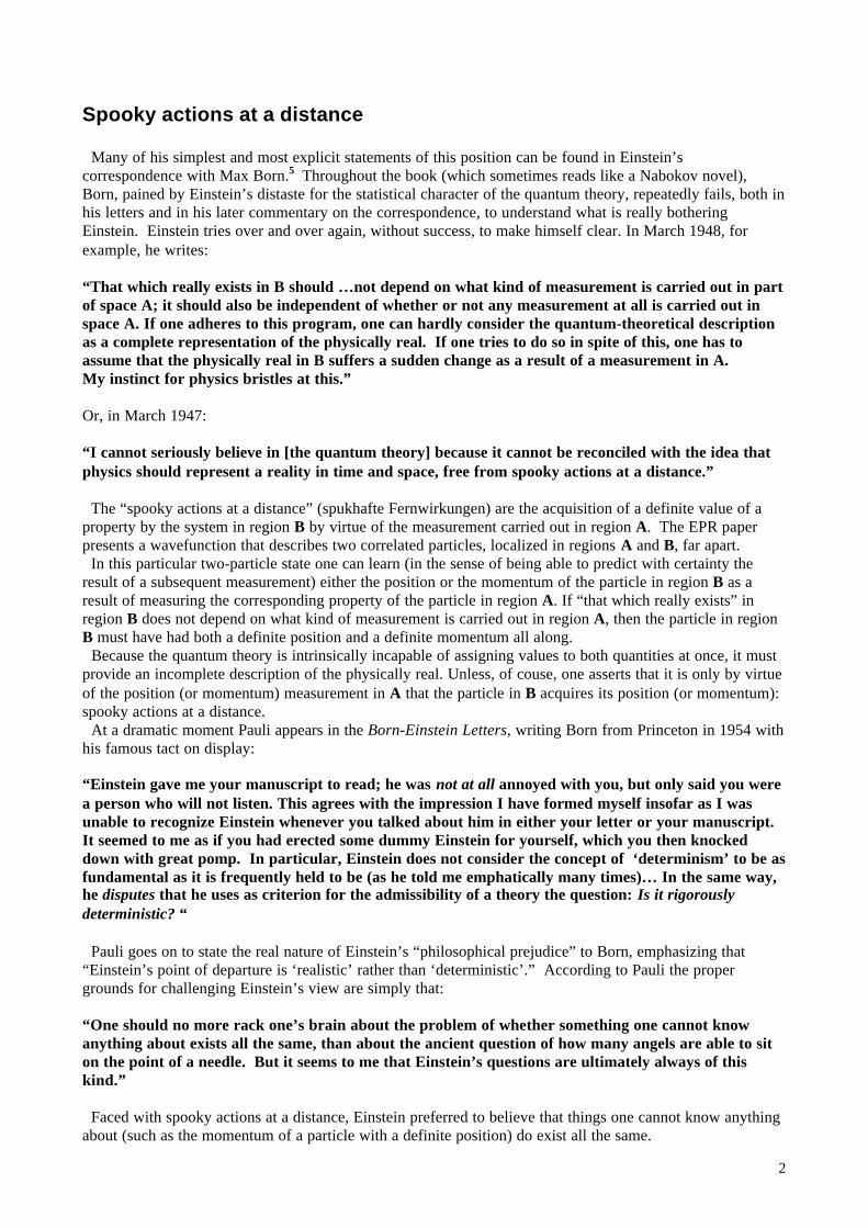
Many of his simplest and most explicit statements of this position can be found in Einstein’scorrespondence with Max Born.5 Throughout the book (which sometimes reads like a Nabokov novel),Born, pained by Einstein’s distaste for the statistical character of the quantum theory, repeatedly fails, both inhis letters and in his later commentary on the correspondence, to understand what is really botheringEinstein. Einstein tries over and over again, without success, to make himself clear. In March 1948, forexample, he writes:

“That which really exists in B should …not depend on what kind of measurement is carried out in partof space A; it should also be independent of whether or not any measurement at all is carried out inspace A. If one adheres to this program, one can hardly consider the quantum-theoretical descriptionas a complete representation of the physically real. If one tries to do so in spite of this, one has toassume that the physically real in B suffers a sudden change as a result of a measurement in A.My instinct for physics bristles at this.”

Or, in March 1947:

“I cannot seriously believe in [the quantum theory] because it cannot be reconciled with the idea thatphysics should represent a reality in time and space, free from spooky actions at a distance.”

The “spooky actions at a distance” (spukhafte Fernwirkungen) are the acquisition of a definite value of aproperty by the system in region B by virtue of the measurement carried out in region A. The EPR paperpresents a wavefunction that describes two correlated particles, localized in regions A and B, far apart. In this particular two-particle state one can learn (in the sense of being able to predict with certainty theresult of a subsequent measurement) either the position or the momentum of the particle in region B as aresult of measuring the corresponding property of the particle in region A. If “that which really exists” inregion B does not depend on what kind of measurement is carried out in region A, then the particle in regionB must have had both a definite position and a definite momentum all along. Because the quantum theory is intrinsically incapable of assigning values to both quantities at once, it mustprovide an incomplete description of the physically real. Unless, of couse, one asserts that it is only by virtueof the position (or momentum) measurement in A that the particle in B acquires its position (or momentum):spooky actions at a distance. At a dramatic moment Pauli appears in the Born-Einstein Letters, writing Born from Princeton in 1954 withhis famous tact on display:

“Einstein gave me your manuscript to read; he was not at all annoyed with you, but only said you werea person who will not listen. This agrees with the impression I have formed myself insofar as I wasunable to recognize Einstein whenever you talked about him in either your letter or your manuscript.It seemed to me as if you had erected some dummy Einstein for yourself, which you then knockeddown with great pomp. In particular, Einstein does not consider the concept of ‘determinism’ to be asfundamental as it is frequently held to be (as he told me emphatically many times)… In the same way,he disputes that he uses as criterion for the admissibility of a theory the question: Is it rigorouslydeterministic? “

Pauli goes on to state the real nature of Einstein’s “philosophical prejudice” to Born, emphasizing that“Einstein’s point of departure is ‘realistic’ rather than ‘deterministic’.” According to Pauli the propergrounds for challenging Einstein’s view are simply that:

“One should no more rack one’s brain about the problem of whether something one cannot knowanything about exists all the same, than about the ancient question of how many angels are able to siton the point of a needle. But it seems to me that Einstein’s questions are ultimately always of thiskind.”

Faced with spooky actions at a distance, Einstein preferred to believe that things one cannot know anythingabout (such as the momentum of a particle with a definite position) do exist all the same.

3

In April 1948 he wrote to Born:

“Those physicists who regard the descriptive methods of quantum mechanics as definitive in principlewould…drop the requirement for the independent existence of the physical reality present in differentparts of space; they would be justified in pointing out that the quantum theory nowhere makes explicituse of this requirement. I admit this, but would point out: when I consider the the physicalphenomena known to me, and especially those which are being so successfully encompassed byquantum mechanics, I still cannot find any fact anywhere which would make it appear likey that [the]requirement will have to be abandoned. I am therefore inclined to believe that the description ofquantum mechanics…has to be regarded as an incomplete and indirect description of reality…”

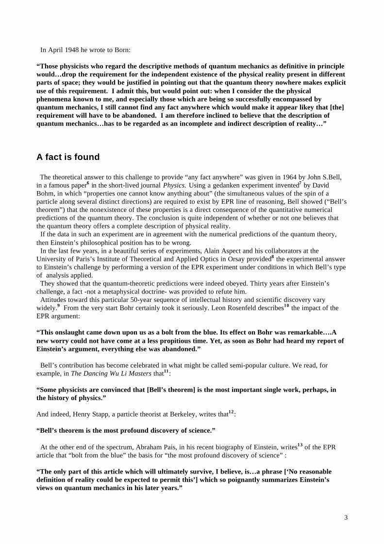
A fact is found

The theoretical answer to this challenge to provide “any fact anywhere” was given in 1964 by John S.Bell,in a famous paper6 in the short-lived journal Physics. Using a gedanken experiment invented7 by DavidBohm, in which “properties one cannot know anything about” (the simultaneous values of the spin of aparticle along several distinct directions) are required to exist by EPR line of reasoning, Bell showed (“Bell’stheorem”) that the nonexistence of these properties is a direct consequence of the quantitative numericalpredictions of the quantum theory. The conclusion is quite independent of whether or not one believes thatthe quantum theory offers a complete description of physical reality. If the data in such an experiment are in agreement with the numerical predictions of the quantum theory,then Einstein’s philosophical position has to be wrong. In the last few years, in a beautiful series of experiments, Alain Aspect and his collaborators at theUniversity of Paris’s Institute of Theoretical and Applied Optics in Orsay provided8 the experimental answerto Einstein’s challenge by performing a version of the EPR experiment under conditions in which Bell’s typeof analysis applied. They showed that the quantum-theoretic predictions were indeed obeyed. Thirty years after Einstein’schallenge, a fact -not a metaphysical doctrine- was provided to refute him. Attitudes toward this particular 50-year sequence of intellectual history and scientific discovery varywidely.9 From the very start Bohr certainly took it seriously. Leon Rosenfeld describes10 the impact of theEPR argument:

“This onslaught came down upon us as a bolt from the blue. Its effect on Bohr was remarkable….Anew worry could not have come at a less propitious time. Yet, as soon as Bohr had heard my report ofEinstein’s argument, everything else was abandoned.”

Bell’s contribution has become celebrated in what might be called semi-popular culture. We read, forexample, in The Dancing Wu Li Masters that11:

“Some physicists are convinced that [Bell’s theorem] is the most important single work, perhaps, inthe history of physics.”

And indeed, Henry Stapp, a particle theorist at Berkeley, writes that12:

“Bell’s theorem is the most profound discovery of science.”

At the other end of the spectrum, Abraham Pais, in his recent biography of Einstein, writes13 of the EPRarticle that “bolt from the blue” the basis for “the most profound discovery of science” :

“The only part of this article which will ultimately survive, I believe, is…a phrase [‘No reasonabledefinition of reality could be expected to permit this’] which so poignantly summarizes Einstein’sviews on quantum mechanics in his later years.”

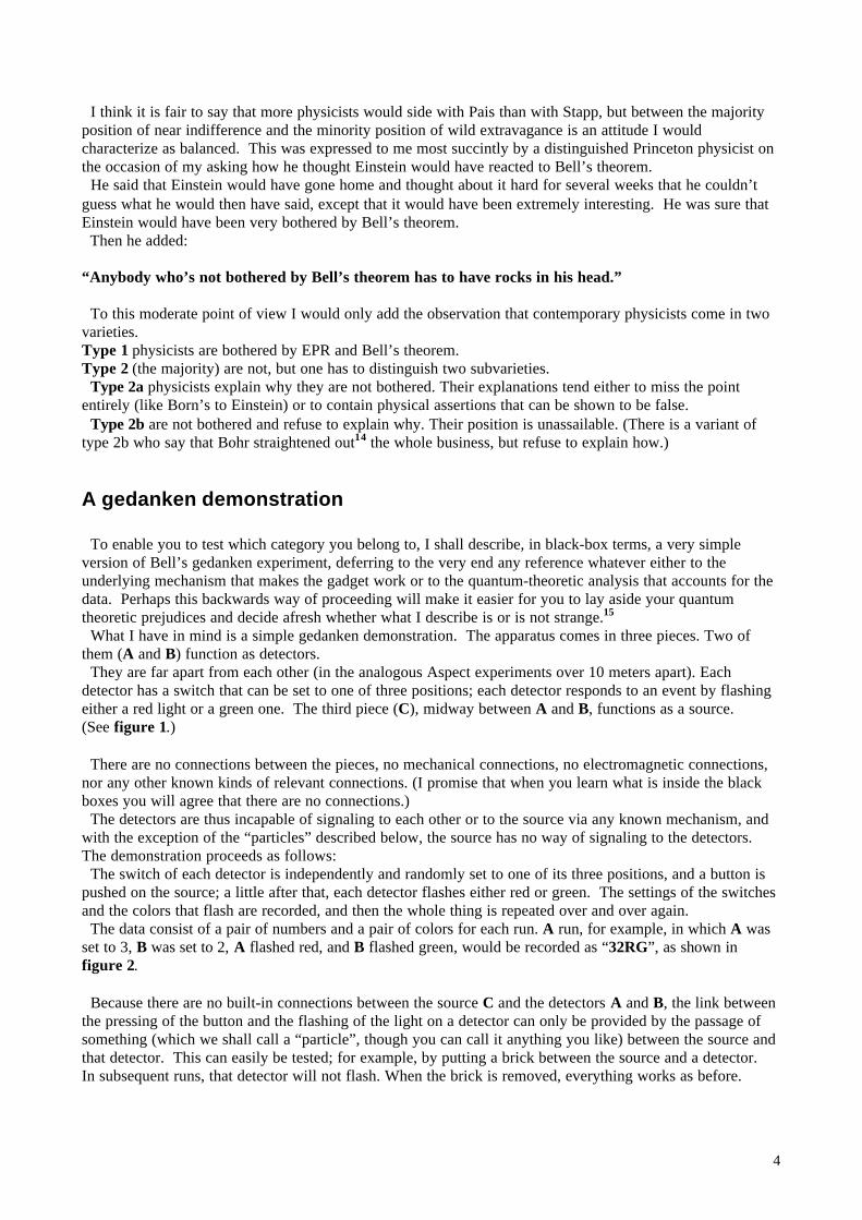
4

I think it is fair to say that more physicists would side with Pais than with Stapp, but between the majorityposition of near indifference and the minority position of wild extravagance is an attitude I wouldcharacterize as balanced. This was expressed to me most succintly by a distinguished Princeton physicist onthe occasion of my asking how he thought Einstein would have reacted to Bell’s theorem. He said that Einstein would have gone home and thought about it hard for several weeks that he couldn’tguess what he would then have said, except that it would have been extremely interesting. He was sure thatEinstein would have been very bothered by Bell’s theorem. Then he added:

“Anybody who’s not bothered by Bell’s theorem has to have rocks in his head.”

To this moderate point of view I would only add the observation that contemporary physicists come in twovarieties.Type 1 physicists are bothered by EPR and Bell’s theorem.Type 2 (the majority) are not, but one has to distinguish two subvarieties. Type 2a physicists explain why they are not bothered. Their explanations tend either to miss the pointentirely (like Born’s to Einstein) or to contain physical assertions that can be shown to be false. Type 2b are not bothered and refuse to explain why. Their position is unassailable. (There is a variant oftype 2b who say that Bohr straightened out14 the whole business, but refuse to explain how.)

A gedanken demonstration

To enable you to test which category you belong to, I shall describe, in black-box terms, a very simpleversion of Bell’s gedanken experiment, deferring to the very end any reference whatever either to theunderlying mechanism that makes the gadget work or to the quantum-theoretic analysis that accounts for thedata. Perhaps this backwards way of proceeding will make it easier for you to lay aside your quantumtheoretic prejudices and decide afresh whether what I describe is or is not strange.15

What I have in mind is a simple gedanken demonstration. The apparatus comes in three pieces. Two ofthem (A and B) function as detectors. They are far apart from each other (in the analogous Aspect experiments over 10 meters apart). Eachdetector has a switch that can be set to one of three positions; each detector responds to an event by flashingeither a red light or a green one. The third piece (C), midway between A and B, functions as a source.(See figure 1.)

There are no connections between the pieces, no mechanical connections, no electromagnetic connections,nor any other known kinds of relevant connections. (I promise that when you learn what is inside the blackboxes you will agree that there are no connections.) The detectors are thus incapable of signaling to each other or to the source via any known mechanism, andwith the exception of the “particles” described below, the source has no way of signaling to the detectors.The demonstration proceeds as follows: The switch of each detector is independently and randomly set to one of its three positions, and a button ispushed on the source; a little after that, each detector flashes either red or green. The settings of the switchesand the colors that flash are recorded, and then the whole thing is repeated over and over again. The data consist of a pair of numbers and a pair of colors for each run. A run, for example, in which A wasset to 3, B was set to 2, A flashed red, and B flashed green, would be recorded as “32RG”, as shown infigure 2.

Because there are no built-in connections between the source C and the detectors A and B, the link betweenthe pressing of the button and the flashing of the light on a detector can only be provided by the passage ofsomething (which we shall call a “particle”, though you can call it anything you like) between the source andthat detector. This can easily be tested; for example, by putting a brick between the source and a detector.In subsequent runs, that detector will not flash. When the brick is removed, everything works as before.

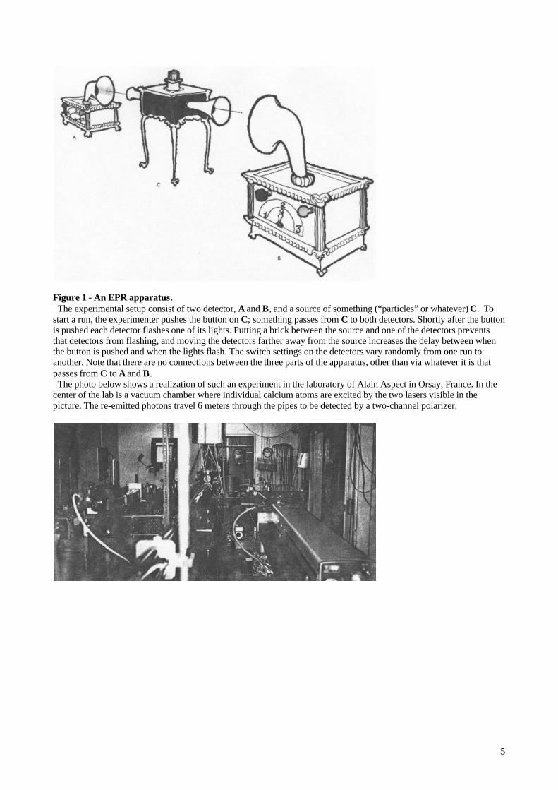
5

Figure 1 - An EPR apparatus. The experimental setup consist of two detector, A and B, and a source of something (“particles” or whatever) C. Tostart a run, the experimenter pushes the button on C; something passes from C to both detectors. Shortly after the buttonis pushed each detector flashes one of its lights. Putting a brick between the source and one of the detectors preventsthat detectors from flashing, and moving the detectors farther away from the source increases the delay between whenthe button is pushed and when the lights flash. The switch settings on the detectors vary randomly from one run toanother. Note that there are no connections between the three parts of the apparatus, other than via whatever it is thatpasses from C to A and B. The photo below shows a realization of such an experiment in the laboratory of Alain Aspect in Orsay, France. In thecenter of the lab is a vacuum chamber where individual calcium atoms are excited by the two lasers visible in thepicture. The re-emitted photons travel 6 meters through the pipes to be detected by a two-channel polarizer.

6

Figure 2 - The result of a run. Shortly after the experimenter pushed the button on the source in figure 1, the detectors flash one lamp each. Theexperimenter records the switch settings and the colors of the lamps and then repeats the experiment. Here, for example,the record reads 32RG –the switches are in positions 3 and 2 and the lamps flashed R and G, respectively.

31RR 12GR 23GR 13RR 33RR 12RR 22RR 32RG 13GG22GG 23GR 33RR 13GG 31RG 31RR 33RR 32RG 32RR31RG 33GG 11RR 12GR 33GG 21GR 21RR 22RR 31RG33GG 11GG 23RR 32GR 12GR 12RG 11GG 31RG 21GR12RG 13GR 22GG 12RG 33RR 31GR 21RR 13GR 23GR

Figure 3 – Data produced by the apparatus. This is a fragment of an enormous set of data generated by many, many runs: each entry shows the switch settings andthe colors of the lights that flashed for a run. The switch settings are changed randomly from run to run.


Figure 4 – Switches set the same. The data of figure 3, but highlighted to pick out those runs in which both detectors had the same switch settings as theyflashed. Note that in such runs the lights always flash the same colors.


Figure 5 – Switches set any way. The data of figure 3, but highlighted to emphasize only the colors of the lights that flashed in each run, no matter howthe switches were set when the lights flashed. Note that the pattern of colors is completely random.

7

Typical data from a large number of runs are shown in figure 3. There are just two relevant features:

I) If one examines only those runs in which the switches have the same setting (figure 4), then onefinds that the lights always flash the same colors.

II) If one examines all runs , without any regard to how the switches are set (figure 5), then one findsthat the pattern of flashing is completely random. In particular, half the time the lights flash thesame colors, and half the time different colors.

That is all there is to the gedanken demonstration.Should you be bothered by these data unless you have rocks in your head ?

How could it work ?

Consider only those runs in which the switches had the same setting when the particles went through thedetectors. In all such runs the detectors flash the same colors. If they could communicate, it would bechild’s play to make the detectors flash the same colors when their switches had the same setting, but theyare completely unconnected. Nor can they have been preprogrammed always to flash the same colors,regardless of what is going on, because the detectors are observed to flash different colors in at least some ofthose runs in which their switches are differently set, and the switch settings are independent random events. How, then, are we to account for the first feature of the data? No problem at all. Born, in fact, in a letter ofMay 1948, offers5 such an explanation to Einstein:

“It seems to me that your axiom of the ‘independence of spatially separated objects A and B’ is not asconvincing as you make out. It does not take into account the fact of coherence; objects far apart inspace which have a common origin need not be independent. I believe that this cannot be denied andsimply has to be accepted. Dirac has based his whole book on this.”

In our case the detectors are triggered by particles that have a common origin at the source C. It is theneasy to dream up any number of explanations for the first feature of the data. Suppose, for example, that what each particle encounters as it enters its detector is a target (figure 6)divided into eight regions, labeled RRR, RRG, RGR, RGG, GRR, GRG, GGR, and GGG. Suppose eachdetector is wired so that if a particle lands in the GRG bin, the detector flips into a mode in which the lightflashes G if the switch is set to 1, R if it is set to 2, and G if it is set to 3; RGG leads to a mode with R for 1and G for 2 and 3, and so on. We can then easily account for the fact that the lights always flash the samecolors when the switches have the same settings by assuming that in each run the source always fires itsparticles into bins with the same labels. Evidently this is not the only way. One could imagine that particles come in eight varieties: cubes, spheres,tetrahedra,… All settings produce R when a cube is detected, a sphere results in R for settings 1 and 2, G forsetting 3, and so forth. The first feature of the data is then accounted for if the two particles produced by thesource in each run are always both of the same variety. Common to all such explanations is the requirement that each particle should, in one way or another, carryto its detector a set of instructions for how it is to flash for each of the three possible switch settings, and thatin any run of the experiment both particles should carry the same instruction sets:I) A set of instructions that covers each of the three possible settings is required because there is no

communication between the source and the detectors other than the particles themselves. In runs inwhich the switches have the same setting, the particles cannot know whether that setting will be 11, 22,or 33. For the detectors always to flash the same colors when the switches have the same setting, theparticles must carry instructions that specify colors for each of the three possibilities.

II) The absence of communication between source and detectors also requires that the particles carry suchinstruction sets in every run of the experiment –even those in which the switches end up with differentsettings- because the particles always have to be prepared: any run may turn out to be one in which theswitches end up with the same settings.

This generic explanation is pictured schematically in figure 7.

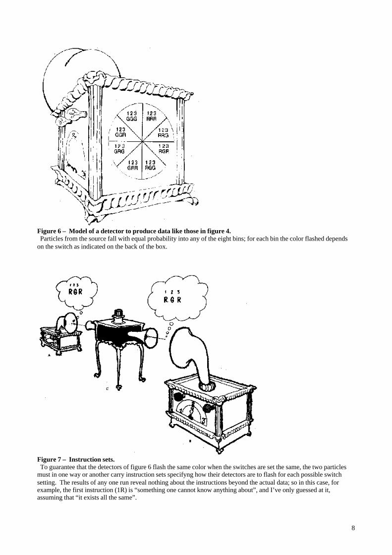
8

Figure 6 – Model of a detector to produce data like those in figure 4. Particles from the source fall with equal probability into any of the eight bins; for each bin the color flashed dependson the switch as indicated on the back of the box.

Figure 7 – Instruction sets. To guarantee that the detectors of figure 6 flash the same color when the switches are set the same, the two particlesmust in one way or another carry instruction sets specifyng how their detectors are to flash for each possible switchsetting. The results of any one run reveal nothing about the instructions beyond the actual data; so in this case, forexample, the first instruction (1R) is “something one cannot know anything about”, and I’ve only guessed at it,assuming that “it exists all the same”.

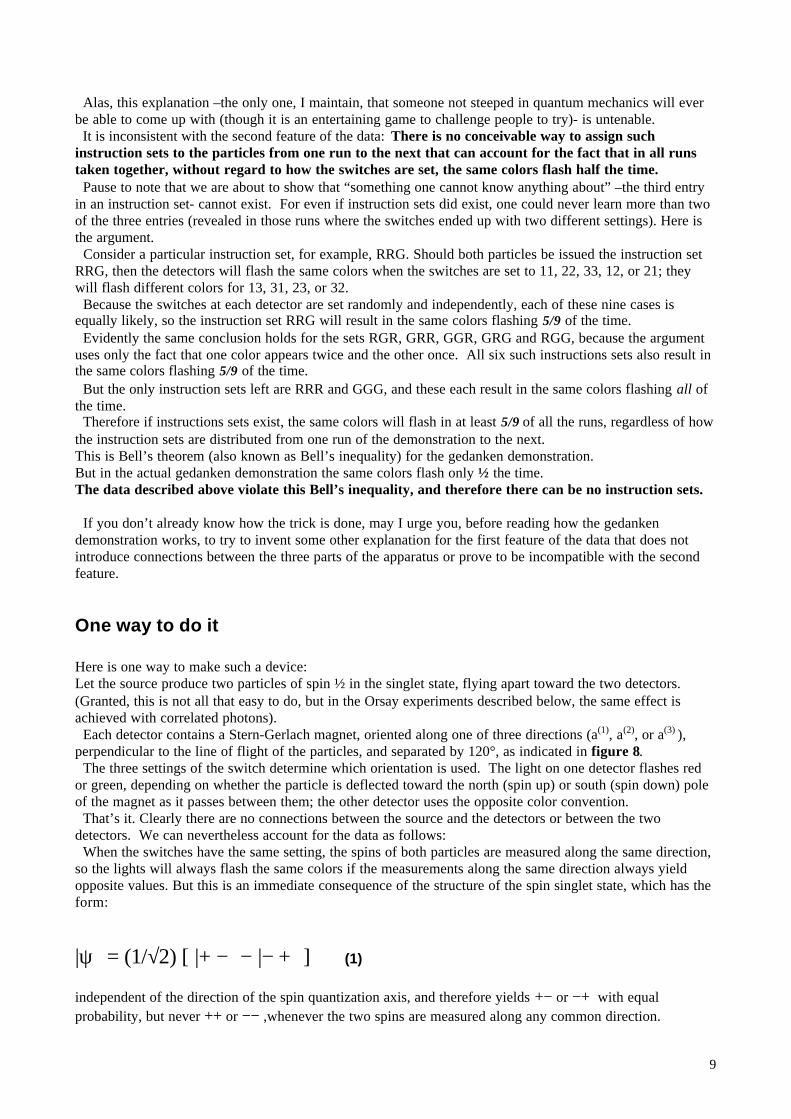
9

Alas, this explanation –the only one, I maintain, that someone not steeped in quantum mechanics will everbe able to come up with (though it is an entertaining game to challenge people to try)- is untenable. It is inconsistent with the second feature of the data: There is no conceivable way to assign suchinstruction sets to the particles from one run to the next that can account for the fact that in all runstaken together, without regard to how the switches are set, the same colors flash half the time. Pause to note that we are about to show that “something one cannot know anything about” –the third entryin an instruction set- cannot exist. For even if instruction sets did exist, one could never learn more than twoof the three entries (revealed in those runs where the switches ended up with two different settings). Here isthe argument. Consider a particular instruction set, for example, RRG. Should both particles be issued the instruction setRRG, then the detectors will flash the same colors when the switches are set to 11, 22, 33, 12, or 21; theywill flash different colors for 13, 31, 23, or 32. Because the switches at each detector are set randomly and independently, each of these nine cases isequally likely, so the instruction set RRG will result in the same colors flashing 5/9 of the time. Evidently the same conclusion holds for the sets RGR, GRR, GGR, GRG and RGG, because the argumentuses only the fact that one color appears twice and the other once. All six such instructions sets also result inthe same colors flashing 5/9 of the time. But the only instruction sets left are RRR and GGG, and these each result in the same colors flashing all ofthe time. Therefore if instructions sets exist, the same colors will flash in at least 5/9 of all the runs, regardless of howthe instruction sets are distributed from one run of the demonstration to the next.This is Bell’s theorem (also known as Bell’s inequality) for the gedanken demonstration.But in the actual gedanken demonstration the same colors flash only ½ the time.The data described above violate this Bell’s inequality, and therefore there can be no instruction sets.

If you don’t already know how the trick is done, may I urge you, before reading how the gedankendemonstration works, to try to invent some other explanation for the first feature of the data that does notintroduce connections between the three parts of the apparatus or prove to be incompatible with the secondfeature.

One way to do it

Here is one way to make such a device:Let the source produce two particles of spin ½ in the singlet state, flying apart toward the two detectors.(Granted, this is not all that easy to do, but in the Orsay experiments described below, the same effect isachieved with correlated photons). Each detector contains a Stern-Gerlach magnet, oriented along one of three directions (a(1), a(2), or a(3) ),perpendicular to the line of flight of the particles, and separated by 120°, as indicated in figure 8. The three settings of the switch determine which orientation is used. The light on one detector flashes redor green, depending on whether the particle is deflected toward the north (spin up) or south (spin down) poleof the magnet as it passes between them; the other detector uses the opposite color convention. That’s it. Clearly there are no connections between the source and the detectors or between the twodetectors. We can nevertheless account for the data as follows: When the switches have the same setting, the spins of both particles are measured along the same direction,so the lights will always flash the same colors if the measurements along the same direction always yieldopposite values. But this is an immediate consequence of the structure of the spin singlet state, which has theform:

|ψ⟩ = (1/√2) [ |+ −⟩ − |− +⟩ ] (1)

independent of the direction of the spin quantization axis, and therefore yields +− or −+ with equalprobability, but never ++ or −− ,whenever the two spins are measured along any common direction.

10

To establish the second feature of the data, note that the product m1m2 of the results of the two spinmeasurements (each of which can have the values +½ or –½ ) will have the value –¼ when the lights flashthe same colors and +¼ when they flash different colors. We must therefore show that the product vanisheswhen averaged over all the nine distinct pairs of orientations the two Stern-Gerlach magnets can have. For a given pair of orientation, a(i) and a(j) , the mean value of this product is just the expectation value in thestate ψ of the corresponding product of (commuting) hermitian observables a(i) ⋅ S(1) and a(j) ⋅ S(2) . Thus the second feature of the data requires:

0 = ∑ij ⟨ψ| [a( i ) ⋅ S( 1 )][a( j ) ⋅ S( 2 )] |ψ⟩ (2)

But equation 2 is an immediate consequence of the linearity of quantum mechanics, which lets one take thesums inside the matrix element, and the fact that the three unit vectors around an equilateral triangle sum tozero:

∑i a( i ) = ∑j a

( j ) = 0 (3)

This completely accounts for the data. It also unmasks the gedanken demonstration as a simpleembellishment of Bohm’s version of the EPR experiment. If we kept only runs in which the switches had thesame setting, we would have precisely the Bohm-EPR experiment. The assertion that instruction sets exist isthen blatant quantum-theoretic nonsense, for it amounts to the insistence that each particle has stamped on itin advance the outcome of the measurements of three different spin components corresponding tononcommuting observables S ⋅ a(i) , i=1,2,3. According to EPR, this is merely a limitation of the quantum-theoretic formalism, because instruction sets are the only way to account for the first feature of the data. Bell’s analysis adds to the discussion those runs in which the switches have different settings, extracts thesecond feature of the data as a further elementary prediction of quantum mechanics, and demonstrates thatany set of data exhibiting this feature is incompatible with the existence of the instruction sets apparentlyrequired by the first feature, quite independently of the formalism used to explain the data, and quiteindependently of any doctrines of quantum theology.

The experiments

The experiments of Aspect and his colleagues at Orsay confirm that the quantum-theoretic predictions forthis experiment are in fact realized, and that the conditions for observing the results of the experiment can infact be achieved. (A distinguished colleague once told me that the answer to the EPR paradox was thatcorrelations in the singlet state could never be maintained over macroscopic distances –that anything, eventhe passage of a cosmic ray in the next room, would disrupt the correlations enough to destroy the effect). In these experiments the two spin ½ particles are replaced by a pair of photons and the spin measurementsbecome polarization measurements. The photon pairs are emitted by calcium atoms in a radiative cascade after suitable pumping by lasers.Because the initial and final atomic states have J=0, quantum theory predicts (and experiment confirms) thatthe photons will be found to have the same polarizations (lights flashing the same colors in the analogousgedanken experiment) if they are measured along the same direction –feature number 1. But if the polarizations are measured at 120° angles, then theory predicts (and experiment confirms) thatthey will be the same only a quarter of the time [ ¼ = cos2 (120°)]. This is precisely what is needed to produce the statistics of feature number 2 of the gedankendemonstration: the randomly set switches end up with the same setting (same polarizations measured) 1/3 ofthe time, so in all runs the same colors will flash 1/3 x 1 + 2/3 x (1/4 ) = ½ the time.

11

Figure 8 – A realization of the detector to produce the data of figure 3. The particles have a magnetic moment and can be separated into “spin up” and “spin down” particles by the Stern-Gerlach magnet inside the detector. Setting the switch to positions 1,2, or 3 rotates the north pole of the magnet alongthe coplanar unit vectors a(1), a(2), or a(3), separated by 120°. The vector sum of the three unit vectors is, of course, zero.The switch positions on the two detectors correspond to the same orientations of the magnetic field. One detectorflashes red for spin up, green for spin down; the other uses the opposite color convention.

The people in Orsay were interested in a somewhat modified version of Bell’s argument in which the anglesof greatest interest were multiples of 22.5°, but they collected data for many different angles, and, except forEPR specialists, the conceptual differences between the two cases are minor.16

There are some remarkable features to these experiments. The two polarization analyzers were placed as faras 13 meters apart without producing any noticeable change in the results, thereby closing the loophole thatthe strange quantum correlations might somehow diminish as the distance between regions A and B grew tomacroscopic proportions. At such separations it is hard to imagine that a polarization measurement of photon#1 could, in any ordinary sense of the term, “disturb” photon #2. Indeed, at these large separations, a hypothetical disturbance originating when one photon passed throughits analyzer could only reach the other analyzer in time to affect the outcome of the second polarizationmeasurement if it traveled at a superluminal velocity. In the third paper of the Orsay group’s series, bizarre conspiracy theories are dealt a blow by an ingeniousmechanism for rapidly switching the directions along which the polarizations of each photon are measured. Each photon passes to its detector through a volume of water that supports an ultrasonic standing wave.Depending on the instantaneous amplitude of the wave, the photon either passes directly into a polarizer withone orientation or is Bragg reflected into another with a different orientation. The standing waves that determine the choice of orientation at each detector are independently driven andhave frequencies so high that several cycles take place during the light travel time from one detector to theother. (This corresponds to a refinement of the gedanken demonstration in which, to be absolutely safe, theswitches are not given their random settings until after the particles have departed from their commonsource).

12

What does it mean ?

What is one to make of all this? Are there “spooky actions at a distance” ?A few years ago I received the text of a letter from the executive director of a California think-tank to theUnder-Secretary of Defense for Research and Engineering, alerting him to the EPR correlations:

“If in fact we can control the faster-than-light nonlocal effect, it would be possible…to make anuntappable and unjammable command-control-communication system at very high bit rates for use inthe submarine fleet. The important point is that since there is no ordinary electromagnetic signallinking the encoder with the decoder in such a hypothetical system, there is nothing for the enemy totap or jam. The enemy would have to have actual possession of the “black box” decoder to interceptthe message, whose reliability would not depend on separation from the encoder nor on ocean orweather conditions….”

Heady stuff indeed! But just what is this nonlocal effect? Using the language of the gedankendemonstration, let us talk about the “N-color” of a particle (N can be 1, 2, or 3) as the color (red or green) ofthe light that flashes when the particle passes through a detector with its switch set to N. Because instruction set cannot exist, we know that a particle cannot at the same time carry a definite 1-color, 2-color and 3-color to its detector. On the other hand, for any particular N (say 3), we can determinethe 3-color of the particle heading for detector A before it gets there by arranging things so that the otherparticle first reaches detector B, where its 3-color is measured. If the particle at B was 3-colored red, the particle at A will turn out to be 3-colored red, and green at Bmeans green at A.Three questions now arise:I) Did the particle at A have its 3-color prior to the measurement of the 3-color of the particle at B? The

answer cannot be yes, because, prior to the measurement of the 3-color at B, it is altogether possiblethat the roll of the dice at B or the whim of the B-operator will result in the 2-color or the 1-color beingmeasured at B instead. Barring the most paranoid of conspiracy theories, “prior to the measurement ofthe 3-color at B” is indistinguishable from “prior to the measurement of the 2- (or 1-) color at B”. If the3-color already existed, so also must the 2- and 1-colors have existed. But instruction sets (whichconsist of a specification of the 1-, 2-, and 3-colors) do not exist.

II) Is the particle at A 3-colored red after the measurement at B shows the color red? The answer is surelyyes, because under these circumstances it is invariably a particle that will cause the detector at A to flashred.

III) Was something (the value of its 3-color) transmitted to the particle at A as a result of the measurementat B?

Orthodox quantum metaphysicians would, I believe, say no, nothing has changed at A as the result of themeasurement at B; what has changed is our knowledge of the particle at A. (Somewhat more spookily, theymight object to the naive classical assumption of localizability or separability implicit in the phrases “at A”and “at B”). This seems very sensible and very reassuring: N-color does not characterize the particle at all, but onlywhat we know about the particle. But does that last sentence sound as good when “particle” is changed to“photon” and “N-color” to “polarization”? And does it really help you to stop wondering why the lightsalways flash the same colors when the switches have the same settings? What is clear is that if there is spooky action at a distance, then, like other spooks, it is absolutely uselessexcept for its effect, begnin or otherwise, on our state of mind. For the statistical pattern of red and green flashes at detector A is entirely random, however the switch is setat detector B. Whether the particles arriving at A all come with definite 3-colors (because the switch at Bwas stuck at 3) or definite 2-colors (because the switch was stuck at 2) or no colors at all (because there wasa brick in front of the detector at B) –all this has absolutely no effect on the statistical distribution of colorsobserved at A. The manifestation of this “action at a distance” is revealed only through a comparison of thedata independently gathered at A and at B.

13

This is a most curious state of affairs, and while it is wrong to suggest that EPR correlations will replacesonar, it seems to me something is lost by ignoring them or shrugging them off. The EPR experiment is as close to magic as any physical phenomenon I know of, and magic should beenjoyed. Whether there is physics to be learned by pondering it is less clear. The most elegant answer I havefound17 to this last question comes from one of the great philosophers of our time, whose view of the matter Ihave taken the liberty of quoting in the form of the poetry it surely is:

We have always had a great deal of difficultyunderstanding the world viewthat quantum mechanics represents.

At least I do,because I’m an old enough manthat I havent’ got to the pointthat this stuff is obvious to me.

Okay, I still get nervous with it….

You know how it always is,every new idea,it takes a generation or twountil it becomes obviousthat there’s no real problem.

I cannot define the real problem,

therefore I suspect there’s no real problem,but I’m not surethere’s no real problem.

Nobody in the 50 years since Einstein, Podolsky and Rosen has ever put it better than that.

[Some of the views expressed above were developed in the course of occasional technical studies of EPR correlationssupported by the National Science Foundation under grant No. DMR 83-14625.]

References

1. Daniel Greenberger, discussion remarks at the Symposium on Fundamental Questions in QuantumMechanics, SUNY, Albany, April 1984.

2. A.Einstein, B.Podolsky, N.Rosen, Phys. Rev. 47, 777 (1935).3. Quoted by M. Jammer, The Philosophy of Quantum Mechanics, Wiley, New York (1974) p.151.4. A.Pais, Rev. Mod. Phys. 51, 863 (1979).5. The Born-Einstein Letters, with comments by M.Born, Walker, New York (1971).6. J.S.Bell, Physics 1, 195 (1964).7. D.Bohm, Quantum Theory, Prentice-Hall, Englewood Cliffs, N.J. (1951) pp. 614-619.8. A.Aspect, P.Grangier, G.Roger, Phys. Rev. Lett. 47, 460 (1981). A.Aspect, P.Grangier, G.Roger, Phys.

Rev. Lett. 49, 91 (1982). A.Aspect, J.Dalibard, G.Roger, Phys. Rev. Lett. 49, 1804 (1982).9. For a discussion of the views of today’s physicists toward the meaning of the quantum theory, see the

interesting and provocative essay “Cognitive Repression in Contemporary Physics” by E.F.Keller, Am.J. Phiys. 47, 718 (1977).

10. L.Rosenfeld in Niels Bohr, His Life and Work as Seen by His Friends and Colleagues, S.Rozental ed.,North Holland, Amsterdam (1967) pp. 114-36.

14

11. G.Zukav, The Dancing Wu-Li Masters –An Overview of the New Physics, Morrow, New York (1979)p.282. On the same page it is also said that “Bell’s theorem is a mathematical construct which as suchis indecipherable to the non-mathematician”, a view that I hope the rest of this article will dispel.

12. H.Stapp, Nuovo Cimento 40B, 191 (1977).13. A.Pais, “Subtle is the Lord…” The Science and the Life of Albert Einstein, Oxford U.P., New York

(1982) p.456.14. N.Bohr, Phys. Rev. 48, 696 (1935).15. What follows is a somewhat refined version of an argument I published a few years ago in Am. J. Phys.

49, 940 (1981), incorporating some improvements suggested by Richard Friedberg. For otherelementary treatments see J.S.Bell’s beautiful essay, “Bertlemann’s Socks and the Nature of Reality”,J. Phys. (Paris) 42, C2-41 (1981), B.d’Espagnat’s article in the November 1979 Scientific American, ord’Espagnat’s recent book, In Search of Reality, Springer-Verlag, New York (1983).

16. For a survey of other attempts to realize the EPR experiment, and the variants of Bell’s originalargument used to interpret experimental tests, see J.F.Clauser, A.Shimony, Repts. Prog. Phys. 41, 1881(1978).

17. R.P.Feynman, Int. J. Theor. Phys. 21, 471 (1982).

Faithful transcription of the original article appeared on PHYSICS TODAY / APRIL 1985 Pag. 38-47

the 1925 born and jordan paper “on quantum mechanics” · pdf filethe 1925 born and...

Documents