textbook - learner of chaos theory. imagine that two leaves, identical in every ... the position of...

TEXTBOOK

UniT 13

THE COnCEPTS OF CHAOS TEXTBOOK

UniT OBJECTiVES

Chaos is a type of nonlinear behavior characterized by sensitive dependence on • initial conditions.

Chaotic systems can be deterministic, yet unpredictable. •

Linear systems are solvable because of superposition. •

Nonlinear systems are often not solvable in an exact sense. •

Phase space is a way to find the qualitative behavior of nonlinear systems. •

Equilibrium points can be stable or unstable. •

Sensitive dependence is easily seen in certain types of iteration procedures. •

The logistic map provides an example of a system that bifurcates into chaos in a • relatively well-understood way.

Space scientists use sensitive dependence to plan minimal-fuel routes through the • solar system.

UniT 13

Physicists like to think that all you have to do is say, these are the conditions, now what happens next?

RICHARD FEYNMAN

Unit 13 | 1

UniT 13 THE COnCEPTS OF CHAOSTEXTBOOK

13.1SECTION

We live in a world in which seemingly insignificant details can have a great impact. Very tiny changes in the starting conditions of a process or procedure can have substantial, sometimes even dramatic, effects on subsequent behavior and results. Some examples presented as evidence of this are purely anecdotal or even theatrical—for example, the train you miss boarding by ten seconds that ends up in a terrible crash—but others are more precise, more scientific, even mathematical. This kind of indeterminacy may seem at odds with the usual mathematical notion of a predictable world. Indeed, for centuries the prevailing view of our universe was that it “runs like clockwork,” and its workings can be mathematically and even numerically predicted from a given set of starting or “initial” conditions. This predictability was possible, supposedly, because we can write equations that tell us exactly (in a perfect world) what to expect, given a set of starting circumstances. However, because we can never know anything exactly—there is always some “error” in perception or measurement—this earlier view of our world carried an implicit assumption that minor discrepancies in the measurement of those beginning circumstances are of little consequence because they should lead to only correspondingly small differences in the predicted results. As it turns out, this view is naive. The real world is one in which small differences in the initial circumstances of a sequence of events can indeed have a significant effect on the final outcome. The mathematical tools that we need to understand this sort of real-world phenomenology come from the realm of chaos theory.

Imagine that two leaves, identical in every way (size, shape, mass, texture, etc.) and attached as closely as possible to each other on the same tree branch, fall at the same time. As the leaves fall, they encounter resistance from the air, with its various eddies and small pockets of higher and lower pressure. These effects cause the two leaves to “dance” in the air as they fall. At times they are close to each other, and at other times they seem to be heading in opposite directions. They finally land in two different locations, each much farther away from the other than when they started.

How can we explain this behavior? The leaves started their descent from virtually the same location and yet ended up far apart. How could such a small difference in starting position lead to such a dramatic difference in final location?

INTRODUCTION

Unit 13 | 2


13.1SECTIONIn a linear world, this sort of behavior shouldn’t happen. Had the two falling objects been apples rather than leaves, we would likely see little, perhaps no, such disparity between their initial and final separation. The density and form of the apples is such that the small shifting wind currents would have virtually no displacement effect. In linear systems such as this, outcomes are always fairly predictable if the initial conditions are known. Small differences in initial conditions, such as the spacing between the apples on the branch, result in only small differences in the eventual outcome, their spacing on the ground.

Leaves, however, are nothing like apples, and their behavior as they fall is anything but easy to explain. Their flight paths are extremely sensitive to small changes in their initial conditions. If the starting point is altered by just the tiniest amount, the path taken by a falling leaf can be entirely different. This is the hallmark of the mathematical concept of chaos.

The mathematics of chaos represents one prong of our endeavor to understand the complicated world around us. This is no small task, given the diverse complexity of our natural world—falling leaves, roiling streams, the rise and fall of species, and of course, that most unpredictable element of nature, the capricious weather. It is not hard to understand why the weather is so unpredictable; it is an extensive and vastly complicated system with many variables, all interacting in subtle ways. What’s startling to realize when studying chaos theory is that even seemingly simple systems can behave in ways that are difficult to predict.

In this chapter we will learn about the mathematics of chaos and how it fits into the broader topic of nonlinear dynamics. Nonlinear dynamics can be thought of as the study of complicated things and complicated behavior. In our previous study of synchronization, we saw how individually complicated things, such as fireflies and heart cells, can behave collectively in strikingly simple ways, such as oscillating in unison. In this unit, we will see how a seemingly simple system, such as that involving a leaf falling from a tree, can exhibit extraordinarily complicated (i.e., difficult to predict) behavior. The broad field of nonlinear dynamics holds much promise for the mathematical understanding of our world. Chaos theory represents some of the first steps toward that understanding.

INTRODUCTIONCOnTinUED

Unit 13 | 3


13.1SECTIONFirst, we will examine the distinction between linear and nonlinear systems. Then, we will explore the notion of predictability. From there, we will examine the fundamental trait of chaotic systems, namely, sensitive dependence on initial conditions. With these notions in hand, we will consider some examples of chaos in action.

INTRODUCTIONCOnTinUED

Unit 13 | 4


SECTION 13.2

Linear vs. Nonlinear• Springs and Things• Good Behavior• Over the Top•

LinEAR VS. nOnLinEARChaos is one of many behaviors that a nonlinear system can display.•

Chaos theory is an often-misunderstood field of mathematics. Many people associate chaos mathematics with the famous “butterfly flapping its wings in China and causing a tornado in Texas” metaphor. This example is well-meaning in that it shows the dependence of large, complicated systems on small changes in initial circumstances. This metaphor is not terribly illuminating regarding chaos theory, however, because the earth’s atmosphere is immensely complicated, with many variables, and it is not too surprising that it behaves in strange ways. Mathematical chaos is most remarkable not because it arises in huge, complicated systems, such as that connected with our planet’s weather, but rather because it appears to be a governing factor even in simple systems, systems that one would think should be fairly predictable but that instead turn out to be chaotic. So in order to observe and study chaos, we do not need a large, complicated system; our only requirement is that our system be nonlinear.

In high school, we learned that a linear equation is any expression of the form y = mx + b, with m and b representing constants (such as 3 and -7) and x and y representing variables, generally called the independent and dependent variables, respectively. The equation is “linear” because its graph (all the “x,y” points on the coordinate plane that satisfy the equation) is a straight line, and also because a small change in the value of x effects a proportional, constant change in y. A nonlinear equation is something that doesn’t have just a first power of the independent variable and consequently can’t be graphed as a simple straight line. One such example is a quadratic equation, ax2 + bx + c = 0.

In our study of chaos, we will need to expand the definitions of linear and nonlinear to include differential equations. Recall from our discussion in the preceding chapter on spontaneous synchronization that a differential equation

LINEAR VS. NONLINEAR SYSTEMS

Unit 13 | 5


SECTION 13.2 is an equation that contains both variables and derivatives, or instantaneous rates of change. A linear differential equation is an equation in which dependent variables and their derivatives appear only to the first power. For example:

5dydt + 4y = 0

This equation is linear because y, the dependent variable (it depends on t), occurs only to the first power, as does its derivative. This differential equation is also linear:

7d2 y

dt2 –

3dydt + 5y = 0

Note that this equation contains a second derivative of the dependent variable, but only to the first power. The following equation also is linear:

3yt2 – 5t5 +

2dydt = 0

Although this equation involves higher powers, they apply only to t, which is the independent variable. The dependent variable, y, and its derivative both appear only to the first power, which is what determines whether or not a differential equation is linear.

Consider this differential equation:

7(

dydt

)2 –

3dydt

+ 5y = 0

This equation contains a derivative raised to the second power, so it is classified as nonlinear. An equation, containing derivatives or not, can be nonlinear in other ways besides containing powers greater than one of dependent variables or derivatives. For example, the following equations are nonlinear:

sin y = 0y + ln y = 0

y +

dydt – 8t(ln y) = 0

A linear system, then, is a set of equations that express a certain physical situation without involving terms that include a dependent variable or the derivatives of that variable to a power greater than one. A nonlinear system is


COnTinUED

Unit 13 | 6


SECTIONlike a linear one, except that one or more terms are nonlinear.The distinction between linear and nonlinear systems in mathematics defines the boundary between the relatively knowable, and the frustratingly elusive. Both types of systems can describe the dynamics of many different processes, such as planets orbiting each other, fluctuations in animal populations, the behavior of electrical circuits, and so on. The difference between linear and nonlinear lies in the details of the equations that govern how these systems interact. For systems that behave linearly, it is relatively easy to find exact solutions that we can use to predict future behavior within the system. For nonlinear systems, we are lucky to find any such solution. Indeed, in nonlinear dynamics, we often have to redefine what we consider to be a solution. Before we get to this new view of solutions, however, let’s take a closer look at the older, linear view.

SPRinGS AnD THinGSA mass on a spring is an example of a simple harmonic oscillator, a well-• understood linear system.Linear systems can be solved relatively simply because they can be broken • down into parts that can be solved separately.

If we attached a weight of mass m to the free end of a spring of strength k that is suspended vertically from a board or the ceiling and allowed the mass to bounce up and down, we would have what is known as a harmonic oscillator. Given an initial displacement (either lifting the mass above or pulling the mass below its resting position), the weight would bounce up and down until the friction of the air, the inelasticity in the spring, and the force of gravity combine to slow the oscillations to a stop. The position of the mass is a dynamical system and is easily defined with this well-known differential equation:

m(

d2x

dt2 ) + b(

dxdt

)+kx =0.

This equation represents the balance of forces acting upon the mass. We know that, given time, the mass will return to rest at its original position; in other words, the forces acting to cause the oscillations must balance out to a zero sum. The first term in the equation comes from Newton’s second law of motion F = ma (force equals mass times acceleration). In our equation, the mass is represented by m and the acceleration is represented by

d2x

dt2 . The second term is the product of the velocity of the mass,

dxdt ,

and some constant, b, that represents the effect of air resistance. The final term represents the force

13.2


COnTinUED

Unit 13 | 7


SECTIONcontributed by the contraction of the spring. This contribution is proportional to how far the spring has been stretched—the more the stretching, the greater the contribution. To find this contribution, we simply multiply the strength of the spring, k, by the amount by which it is stretched, x. We add all these contributions together and set them equal to zero in accordance with Newton’s third law of motion, which states that every action has an equal and opposite reaction.

As this equation is written above, it incorporates both first and second derivatives, making it somewhat difficult to solve directly. We can transform the equation to one without a second derivative and, hence, one more easily solved by performing a change of variables. To do this, we must first recognize that

d2x

dt2 is just the first derivative of

dxdt . If we let x = x1, and

dxdt = x2, then

d2x1

dt2 becomes

dx2

dt. With the second derivative conveniently eliminated, we can now

write a system of equations to model our oscillator:

dx1

dt= x2

m(

dx2

dt) + b x2 + k x1 = 0

We can rewrite this as:

dx1

dt = x2

dx2

dt= (

–bm

) x2 – (

km

)x1

This is a linear system because all of its terms are single, first-degree variables with constant coefficients. We need not work through the details of the solution to this system. It is important to realize, however, that it would be some function x(t) that describes where the mass would be at any time, t, that we choose. The solution is an equation that can be used to determine the exact location of the mass at any time during its oscillation.

Because this system is linear, we could use the principle of superposition to solve it. This principle enables us to break a system of equations into pieces that are more easily solved, solve them, and then combine the partial solutions to find a solution of the entire system. This is a case of the whole solution being exactly the sum of the partial solutions. Because of the applicability of this principle of superposition, it is relatively easy to get exact, predictive solutions for linear systems.

13.2


COnTinUED

Unit 13 | 8


SECTIONGOOD BEHAViOR

Linear systems tend toward one of four predictable behaviors.•

One nice thing about linear systems is that, because they are exactly solvable, we can categorize the types of behavior that they can exhibit. When we refer to the behavior of a system, what we are really concerned with is the behavior of the variables that describe the state of the system. For our oscillating spring, the pertinent variables are the position of the mass, x, and its velocity, dx/dt. Given these two values, we know exactly what the system is doing at any moment. In general, the variables that describe the state of linear systems can:

1. Grow exponentially, heading toward infinity. An example of this occurs when bacteria are allowed to grow with unlimited resources.

2. Decay exponentially, heading toward zero. A common example is the decay of radioactive materials.

3. Cycle periodically, forever oscillating between values. An example is a harmonic oscillator acting in the absence of friction.

4. Exhibit any combination of the above behaviors. Our mass and spring oscillator acting with friction behaves as a combination of (3) and (2) in sort of a decaying oscillation; it oscillates, but each cycle is shorter than the preceding one until the mass stops moving. Another example of this is the case of a bungee jumper coming to rest at the bottom of her cord.

All four of these behaviors are nice and predictable in the linear view. Unfortunately, most real-life systems are not so well behaved and do not fit well into a linear model.

OVER THE TOPA pendulum swinging outside of the small-angle approximation, where • sin θ ~ θ, is an example of a nonlinear system.For small swings, a pendulum behaves predictably, but for large swings, it • can behave strangely.


COnTinUED

13.2

Unit 13 | 9


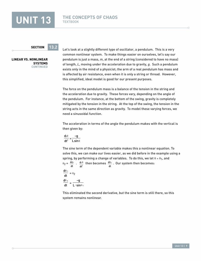
SECTION 13.2 Let’s look at a slightly different type of oscillator, a pendulum. This is a very common nonlinear system. To make things easier on ourselves, let’s say our pendulum is just a mass, m, at the end of a string (considered to have no mass) of length, L, moving under the acceleration due to gravity, g. Such a pendulum exists only in the mind of a physicist; the arm of a real pendulum has mass and is affected by air resistance, even when it is only a string or thread. However, this simplified, ideal model is good for our present purposes.

The force on the pendulum mass is a balance of the tension in the string and the acceleration due to gravity. These forces vary, depending on the angle of the pendulum. For instance, at the bottom of the swing, gravity is completely mitigated by the tension in the string. At the top of the swing, the tension in the string acts in the same direction as gravity. To model these varying forces, we need a sinusoidal function.

The acceleration in terms of the angle the pendulum makes with the vertical is then given by:

d2θdt2 =

–gLsinθ

The sine term of the dependent variable makes this a nonlinear equation. To solve this, we can make our lives easier, as we did before in the example using a spring, by performing a change of variables. To do this, we let θ = θ1, and θ2 =

dθθ1

dt .

d2θdt2

then becomes

dθ2

dt. Our system then becomes:

dθθ1

dt = θ2

dθ2

dt =

–gLθsinθ1

This eliminated the second derivative, but the sine term is still there, so this system remains nonlinear.


COnTinUED

θ

θ

θ

θ

θ θ θ

θ

Unit 13 | 10


SECTIONThese so-called nonlinear systems can exhibit some wild behaviors, behaviors that might be considered surprising, behaviors that don’t fit so nicely into equations. For example, our simple pendulum behaves very smoothly and predictably as long as it doesn’t swing too high.

For larger and larger angles, the range of possible behaviors is more varied than the simple cycling back and forth. For example, if the pendulum has sufficient momentum, it will swing past the horizontal line of the pivot and go all the way around, over the top. If it has a little less momentum than this, it might stall near the vertical position above the pivot, lose the tension of the string, and drop almost straight down under the influence of gravity. Both of these behaviors are examples of nonlinearities. It’s worth noting that for a pendulum to swing higher than its pivot, the mass must have some initial velocity. Velocity due to gravity alone will not suffice. Since we are only concerned with general methods and qualitative behavior, we can ignore this.

Some nonlinear systems do behave nicely and predictably, while others do not. The range of nonlinear behaviors is vast, with chaos being just one type. It’s the type that we understand the best. As we will see in the next section, our understanding of chaos does not mean that we can make exact predictions in a chaotic system, as we can with linear systems. In fact, to go any further in our exploration of chaos we will have to redefine what we even mean by the term “solution.”

13.2


COnTinUED

1761

Small angle Larger angle Larger angle

Unit 13 | 11


SECTION

The Two-Body Problem• Poincaré’s Discovery• Phase Portraits•

THE TWO-BODY PROBLEMNewton calculated the motion of the planets using differential equations for • two objects influencing each other with gravity.Given the initial conditions and the relevant equations, one can predict • where two mutually orbiting objects will be at any point in time.

A common belief toward the end of the 19th century was that mathematics can be used to obtain an exact description of the world around us. The pinnacle of this belief was the doctrine of determinism, which holds that if we can know the state of the universe at one moment, and write out all the equations that govern it, we can accurately predict its state at any other moment in the future.

Much of the impetus for this popular view came from the work of Sir Isaac Newton in formulating both laws of motion and the mathematical techniques of calculus that could be used to make accurate predictions based on those laws. According to the Newtonian view, if one had the proper equations and reasonably accurate knowledge of starting conditions, one could predict the future behavior of a system with extreme accuracy.

This deterministic Newtonian view was, and is still, a powerful paradigm. It fostered mathematical understanding of aspects of the world around us that were previously inaccessible. A key example of the power of this line of thinking was Newton’s solution of the two-body problem.

The two-body problem is a simplified version of the problem of describing the motions of the planets. Numerous philosophers and scientists throughout the centuries had attempted to explain planetary motion. Newton was the first to model these motions mathematically and to make accurate predictions about how the planets move and why.

Newton used his newly formulated law of gravitation to model the forces that two massive bodies exert on each other. Plugging quantitative values for these forces into his equations of motion, Newton was able to predict how the two

13.3

LIMITS OF PREDICTABILITY

Unit 13 | 12


SECTIONobjects would move with respect to one another. He found a number of different possible orbits that depended on specific conditions such as the masses of the bodies, their separation distance, and their initial velocities. In short, he found that any system of two orbiting bodies exhibits one of two possible behaviors. The two bodies either settle into a periodic orbit, cycling between positions forever, or they affect each other only briefly and then separate along asymptotic paths, in much the same way that a meteor shoots past a planet. According to Newton, the specific starting values of the system determined which one of these behaviors would occur. Once the system was quantified and put in motion, its fate was known and there were no surprises.

POinCARé’S DiSCOVERYThe three-body problem is very different from the two-body problem.• Poincaré showed that the behavior of a three-body system cannot be • quantitatively predicted.

The solution of the two-body problem was a triumph of both science and mathematics. It gave hope that if the heavens could be understood mathematically, so could other aspects of life. Perhaps there was a bright future in which much of the unpleasant uncertainty in peoples’ lives could be eliminated. It was assumed that Newton’s methods could be easily extended from a system of two massive bodies to one with three and eventually to systems with any number of bodies. Unfortunately, the “tricks” that Newton applied to generate an exact solution to the two-body problem are not applicable to the three-body problem. Many of the greatest mathematical minds of the 18th and 19th centuries, including Euler and Lagrange, attempted to find a general, exact, solution. The problem of describing the interrelated motion of more than two bodies remained so elusive that the King of Sweden, in the late 19th century, established a prize for its solution. The king phrased his challenge in these terms:

13.3

LIMITS OF PREDICTABILITY COnTinUED

1762

Centerof mass

Orbit

Centerof mass

Orbit Brief interaction

Unit 13 | 13


SECTION“Given a system of arbitrarily many mass points which attract each other according to Newton’s laws, try to find, under the assumption that no two points ever collide, a representation of the coordinates of each point as a series in a variable which is some known function of time and for all of whose values the series converges uniformly.”

The great French mathematician and scientist, Henri Poincaré, tackled this challenge. His response, while not providing the general solution that the king sought, laid the groundwork for what would later be known as chaos theory. He examined a very specific case of the three-body problem, a case in which two of the bodies orbited each other as Newton described, while a third mass-less speck orbited them. The advantage of this purely theoretical model was that the speck exerted no gravitational attraction on the other two bodies.

As he delved into the problem, Poincaré abandoned the goal of finding exact solutions of the type desired by the king and instead focused on studying the qualitative behavior of the system. He realized that an exact solution, as was available in the two-body case, was not possible for the case involving three bodies. Fortunately, he also realized that this did not preclude answering important qualitative questions such as, “Is the system stable or will the planets eventually fly off to infinity?” What he found was that the behavior of the mass-less speck was wildly unpredictable.

Poincaré was able to explore such qualitative features of the system by using the concept of phase space. Phase space is an abstract space of the stated variables of a system. In other words, if you take all the possible combinations of, say, position and velocity and arrange them as coordinates in an abstract space, then a path through this space represents how the system will evolve. The initial conditions of a system correspond to where it starts in phase space.

The actual phase space for the three-body problem is 18-dimensional. Each of the three bodies requires three dimensions to describe its position, x, y, and z, and three dimensions to describe its velocity,

dxdt

,

dydt

, and

dzdt

. By looking only at the mass-less speck and confining its position and velocity to the orbital plane, Poincaré reduced the 18 dimensions to 4: x, y,

dxdt

, and

dydt

. Constraining the total energy of the system eliminates one more variable dimension, leaving a three-dimensional phase space, which is readily visualized.

13.3


Unit 13 | 14


SECTION 13.3

What sorts of information can we infer from a picture such as this? It would be better to look at a simpler example of phase space to get an idea of how we can use it to analyze the qualitative behavior of a system.

PHASE PORTRAiTSA phase portrait is a way to visualize all states of a system.• Using a phase portrait, one can deduce the qualitative features of a • system’s evolution.If a system starts out at an equilibrium point, it will not be driven to change • its state.Equilibria can be stable (attractors) or unstable (repellers).•

A more accessible example of this qualitative method is the phase portrait, which is a specific path or set of paths through a phase space, of a system such as:

dxdt

= sin x

This system describes an object whose position oscillates sinusoidally. Although this system can be solved directly through integration, looking at the phase portrait will tell us more about the actual behavior of the system than would be obvious in an exact solution.


Stable Manifold (orbits move toward the periodic orbit)

Unstable Manifold (orbits move away the periodic orbit)

Poincaré’s phase space for 3-bodies

Unit 13 | 15


SECTION

What this picture portrays is the velocity,

dxdt

, of the system at any given position, x. The arrows on the x-axis serve to remind us of the directional component of the velocity. Values of x that yield positive velocities will move the particle to the right; values of x associated with negative velocities will move it to the left.

The places where our path crosses the x-axis correspond to positions that yield no velocity (because sin(0) = 0). These are known as stability points, because if we started a particle at any of these points, it would not be influenced to move in any direction. There are two main types of equilibrium points, stable and unstable. A stable equilibrium point is one to which a particle would return if it were displaced by some small amount. Think of releasing a grape on the inside rim of a bowl. No matter where you release the grape, it will always end up in the center of the bottom of the bowl. This is a stable equilibrium point. If you were to turn the bowl over and place the grape very carefully in the exact center of its top, the grape would stay where you put it. If you placed it anywhere else on the outside of the bowl, however, it would roll off. All of these possible locations represent unstable equilibrium points.

13.3


dxdt

dxdt

Unit 13 | 16


SECTION

We can determine what kind of equilibrium points we have in our phase portrait by looking at the velocities associated with particle movement around each point. The velocity to the left of point A is positive, driving the particle to the right. The velocity to the right of point A is negative, driving the particle to the left. This means that if a particle starts out anywhere relatively close to point A, it will eventually come to rest at point A. Point A is, therefore, a stable equilibrium point. Because it seems to attract particles, we can call it an attractor.

Point B, on the other hand, is a bit different. The velocities corresponding to positions to its left are negative, tending to drive the particle away from the point. The velocities corresponding to positions to its right are positive, also tending to drive the particle away from point B. This indicates that starting a particle anywhere near point B will result in that particle moving away from that position and toward one of the attractors. Point B is, therefore, an unstable equilibrium point. Because it tends to repel particles, we can call it a repeller.

Examining systems in this way, geometrically, has the advantage of enabling us to see certain aspects of their behavior very clearly, without having to plow through pages of equations. By identifying attractors and repellers, we can tell how a system will evolve qualitatively over time, depending upon where it starts.

13.3


1763

Stable equilibrium

Grape

Bowl

Note a small nudge and the grape returns to the center,

the equilibrium point.

Unstable equilibrium

Grape Bowl

Note a small nudge sendsthe grape away from

the equilibrium point.

Unit 13 | 17


SECTION Although in the preceding example we saw how certain points act as attractors or repellers, this does not always have to be the case. For example, if we look at the phase portrait of a simple harmonic oscillator, such as the mass and spring that we examined previously (but without friction this time), we see that there is a nice closed loop corresponding to each combination of starting position and starting velocity.

Wherever we start our system, we see that it will trace out a path in phase space. This path is like a series of equilibrium points, and the system will naturally evolve toward following this path through phase space. This means that attractors do not have to be single points; instead, they can be paths, or trajectories, through phase space.

This notion of examining phase space was part of the contribution that won Poincaré the prize for the three-body problem. He did not find an exact solution, but his techniques were so important that he won the contest anyway. He found that the three-body system exhibits a range of possible behaviors, including some that seem to be wildly unpredictable; that is, even if you know the state of the system at some point in time, there is no guarantee that you will be able

13.3


1764x

dxdt

Small initialdisplacement

MASS

Large initialdisplacement

MASS

Unit 13 | 18


SECTION to say what the state will be at some significantly later time. In the short term, things are predictable, but in the long term, there is no way to know for sure what will happen.

These initial insights from Poincaré dealt a blow to the Newtonian paradigm of deterministic predictability. Poincaré’s dynamics were still deterministic in the sense that the state of a system at any one time depends on its state at a previous time. However, in opposition to Newton’s viewpoint, they were far from delineating a predictable future. Poincaré’s concept, which represented the first notion of what is now called mathematical chaos, made it clear that there is a limit to how far into the future we can see using mathematics. These ideas, though shocking, did not really take hold until the mid-20th century when the advent of the computer enabled mathematicians to practice mathematics in an entirely new way. With the help of computers, mathematicians soon found another remarkable aspect of chaotic behavior, the idea of sensitive dependence, to which we will now turn.

13.3


Unit 13 | 19


SECTION

Rounding Error• Butterflies•

ROUnDinG ERRORLorenz discovered that a small change in the input to a certain system of • equations resulted in a surprisingly large change in output.

Edward Lorenz is a noted mathematician and meteorologist. Throughout the mid-to-late 20th century he was a meteorological researcher at MIT. In the 1950s and 1960s, the study of meteorology was as much art as it was science. Weather forecasters could find certain patterns in weather systems that were somewhat tame and predictable, but there was always an element of surprise. It was thought that this was simply because the dynamics of the atmosphere were so complex, involving so many variables, that it was impossible to state with any precision at any one time what exactly was going on. Without knowing the initial conditions of the system, it was very hard to make exact predictions about what it would do next.

Lorenz hoped to gain some insight into the complexity of the weather by working with an extremely simplified version of a weather model and running it on the newly available computers. With a computer, he believed that he could have exquisite control over the initial conditions, allowing the modeling equations to function more-or-less free of measurement error. By looking at such an ideal and simplified system, he hoped to get a better idea of the fundamental phenomena that underlie the weather.

After considering a complicated, 12-equation model of how air moves, Lorenz chose to focus on a system employing just three equations, a simple model of convection rolls.

dxdt

= σ(y-x)

dydt

= rx – y – xz

dzdt

= xy – bz

Lorenz’s model represented an extreme simplification of a weather system. Using simplified equations for convection currents, his model simulated various

13.4

SENSITIVE DEPENDENCE

Unit 13 | 20


SECTION winds interacting. In the early days of scientific computing, this was a tedious process. He would input his equations and a set of initial conditions and then have the computer calculate what would happen as time moved forward in discrete steps. To make sense of his model’s output, he would choose a specific variable, such as the direction of the west wind, and plot its behavior graphically. He watched as the wind shifted directions, a phenomenon represented by a wavy-line computer printout. This line represented a record of how that direction of the wind changed according to his mock-up, as calculated by the computer.

As the story goes, one day, he was forced to stop his calculations mid-simulation. When he returned a bit later, he decided to start the simulation again, using the values that had been generated and recorded at its stopping point, rather than starting the simulation over with the initial values. He entered the values from before as the initial conditions and was amazed by what happened. The simulation progressed as predicted for a while, but then quickly and inexplicably diverged from what he had seen in previous simulations.

Lorenz initially suspected that there had been a computer malfunction. In Newtonian determinism, there should be no difference between an interrupted and a non-interrupted test. Upon further investigation and reflection, Lorenz realized that there had been no malfunction; the discrepancy was due to a tiny rounding difference between the computer and the printer that displayed the data.

Lorenz’s computer’s memory was programmed to register six decimal places. For example, at the end of a round of simulation, the computer would output a number such as 0.506127. This number would then automatically be used as the initial condition for the next round of simulation. Lorenz’s printout, on the other hand, displayed only three decimal places (a paper-saving feature), and it was this printout that he used to input the starting values when he re-started the interrupted experiment. Had the computer not been interrupted, it would have continued using the 6-digit number; Lorenz had assumed that inputting a 3-digit approximation would not change the results very much.

The difference between 0.506127 and 0.506 is a little more than one part in ten thousand. This is a miniscule deviation, the kind of discrepancy that scientists regularly ignore because they assume that small errors in input have only small effects on output. Lorenz found, however, that this tiny discrepancy had

13.4


COnTinUED

Unit 13 | 21


SECTIONprofound implications for the long-range behavior of his “simple” system.Lorenz had thought that perhaps computers would be the supreme data processors, capable of generating complete, accurate weather predictions. Nonetheless, he also knew that a computer’s output is only as reliable as its input. Experimental scientists have long known that the initial conditions of a system can never be quantified with 100% accuracy. What Lorenz found in his computer simulations was that a small difference in initial conditions could result in large discrepancies between expected outcomes in certain systems. This concept, which came to be known as sensitive dependence, is the key trait of systems that exhibit chaos. BUTTERFLiES

The phase space of the Lorenz system contains an attractor whose phase • portrait resembles a butterfly.The Lorenz attractor helps to explain how small changes in starting • conditions lead to greater changes down the line.

To understand sensitive dependence a little better, Lorenz decided to look at the phase space of his system. He saw something much more complicated than the simple phase portraits that we observed in the previous section.

13.4


COnTinUED

Unit 13 | 22


SECTIONThis phase portrait is three-dimensional, one dimension for each of the variables in Lorenz’s equations. It represents how Lorenz’s simplified weather system evolves through time. It is an abstract path consisting of points whose coordinates are determined by Lorenz’s equations. If we imagine a particle sliding along this abstract path, that particle’s behavior will be indicative of the behavior of the system in general.

What is remarkable about this object is that if you were to start two different particles off in almost but not quite exactly the same location and then allow them to flow along the curve, they would remain close to each other for a while but would at some point start to diverge in their paths very rapidly. This is just like the example of falling leaves from the introduction to this unit. Although the two leaves start out in almost, but not quite exactly, the same position, we all know that by the time they reach the ground, they can be very far apart indeed. In the present example, note also that the particles, even though they follow different paths, still stay somewhere close to this butterfly pattern. That is another hallmark of chaos: indeterminacy mixed with some notion of determinacy – that is bounded in space. Just as the leaf is sure to hit the ground eventually, chaotic behaviors are confined in their outcomes.

Chaotic unpredictability and sensitive dependence can arise in some nonlinear systems, but not all. They represent just a small part of the broader, mostly untamed, field of nonlinear dynamics. While the initial discoveries of chaotic behavior came from the realm of continuous dynamics, such as the motions of planets, chaos also arises in discrete time situations. Lorenz, for example, made his discovery by examining discrete-time solutions to his differential equations. These are situations in which a process is repeated for several steps, each step using the product of the step before as its initial condition. The mechanics of chaos can be better understood by looking at these iterative functions, and so it is to the subject of iteration that we will now turn our attention.

13.4


COnTinUED

Unit 13 | 23


SECTION

Folding Dough•

FOLDinG DOUGHA simple way to see sensitive dependence is to look at discrete, iterative • processes, such as folding dough.

In everyday life, we rarely perceive any boundary between one moment and the next, but, instead, perceive time as flowing continuously. Some processes, however, can be broken into discrete steps. Folding and kneading dough is a good example of this; each fold is more or less an instantaneous event and the time between folds serves as a boundary.

Folding dough can, therefore, be modeled, approximately, in “discrete time.” You can think of discrete time as something like a sequence of snapshots, whereas continuous time is more like a movie. Discrete time breaks a process up into the inputs and outputs at individual, separated moments in time (or space). A discrete dynamical system generally takes at each moment the output of a given step to be used as the input for the next step in the process. This process is called iteration; complete a step by performing an action that generates a new value, then use that new value as the starting point as you repeat the same action. Repeat this process for as long as you like.

Imagine a flake of pepper on the surface of the dough. As we knead and fold the dough the pepper flake gets moved about, its location changing from discrete moment to the next. A computational analogy would be as follows: We start with a number; “stretch” it; chop off a bit we don’t need; and end up with a new number. The stretching will be accomplished by multiplication, the chopping will be a modular arithmetic action. Our process will be to multiply the starting

13.5

ITERATION

1765 Stretch Fold

Stretch StretchFold

Unit 13 | 24


SECTION number by ten, then take the result, modulo 1. (Recall from the unit on primes and modular arithmetic that “modulo 1” is the mathematical way of saying “remove the integer part.”) This eliminates any whole numbers that might be in the result, leaving only a decimal number to begin the next iteration.

Let’s start our process with a decimal input, 0.506127.

First we stretch it by multiplying by ten:

10 × 0.506127 = 5.061270

Next we take the result mod 1:

5.061270 mod 1 === 0.061270

We now use this result as the starting point for the next iteration:

0.061270 × 10 = 0.612700

0.612700 mod 1 === 0.612700 (no change, because there was no whole number component of the number)

So far so good, but what does this have to do with chaos? If we take two numbers that are almost but not quite exactly the same, say 0.12345 and 0.12349, and perform this iterative stretching and chopping process, we will see the essence of chaos unfold before our eyes. The following table records the evolution of the iterative process, and the image that follows demonstrates the divergence of the two values on a series of number lines.

13.5

ITERATIONCOnTinUED

INPUT 0.12345 0.12349

1st Iteration (10x mod 1) 0.23450 0.23490

2nd Iteration 0.34500 0.34900

3rd Iteration 0.45000 0.49000

4th Iteration 0.50000 0.90000

1132

Unit 13 | 25


SECTION

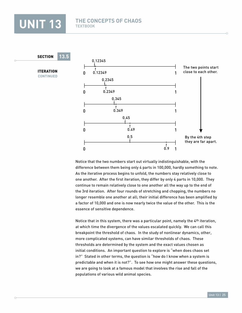
Notice that the two numbers start out virtually indistinguishable, with the difference between them being only 4 parts in 100,000, hardly something to note. As the iterative process begins to unfold, the numbers stay relatively close to one another. After the first iteration, they differ by only 4 parts in 10,000. They continue to remain relatively close to one another all the way up to the end of the 3rd iteration. After four rounds of stretching and chopping, the numbers no longer resemble one another at all; their initial difference has been amplified by a factor of 10,000 and one is now nearly twice the value of the other. This is the essence of sensitive dependence.

Notice that in this system, there was a particular point, namely the 4th iteration, at which time the divergence of the values escalated quickly. We can call this breakpoint the threshold of chaos. In the study of nonlinear dynamics, other, more complicated systems, can have similar thresholds of chaos. These thresholds are determined by the system and the exact values chosen as initial conditions. An important question to explore is “when does chaos set in?” Stated in other terms, the question is “how do I know when a system is predictable and when it is not?”. To see how one might answer these questions, we are going to look at a famous model that involves the rise and fall of the populations of various wild animal species.

13.5

ITERATIONCOnTinUED

1766

0 0.12349

0.12345

1

0 10.2349

0.2345

0 10.349

0.345

0 0.49

0.45

1

0 0.9

The two points startclose to each other.

By the 4th stepthey are far apart.

0.5

1

Unit 13 | 26


SECTION 13.6

Bifurcation• The Road to Chaos• Feigenbaum’s Constants•

BiFURCATiOnA bifurcation is an abrupt change in the qualitative behavior of a system.•

The iterative, discrete-time view of chaos is powerful because it allows us to see how a system evolves, step-by-step. Most nonlinear systems are chaotic only under certain circumstances. A discrete-time analysis can help pin down these circumstances. An example of this is the flow of water, or any fluid. As long as it is allowed to flow at a reasonable speed along a course free of obstacles, fluid flow is nice and predictable. However, as the speed of flow increases, or as obstacles are added in the path of the flow, the flow starts to get somewhat unpredictable. Eventually, under certain conditions, the fluid no longer behaves in a predictable way at all; this condition is called turbulence.

Turbulence is a good deal more complicated and less understood than classic chaos, but the point is that our system changes its qualitative behavior, depending on the specific parameters we assign to it. We expect that using different starting values will give us different results, but we also naturally tend to expect that those results, while different quantitatively, will be somewhat similar qualitatively. We might expect that doubling the weight of a moving particle would halve its velocity, given the same amount of force. We would probably also expect that the particle would still get to where it was headed initially; although it might take longer. In a chaotic system, however, doubling the weight might cause the particle to reverse direction, stop, oscillate between two or more values, or exhibit any number of qualitatively different behaviors.

The point at which a system changes from one fundamental type of behavior to another is called a bifurcation. An important question then is “for what values of our system’s parameters does bifurcation occur?” Applied to our system of moving water, the question is “at what speed does the water flow become turbulent?” Answering this question and others like it is of great importance if you are designing boats, testing aircraft, trying to understand the fluctuations of the stock market, or trying to predict how populations of wild animals rise and fall.

ThE LOgISTIC MAP

Unit 13 | 27


SECTIONTHE ROAD TO CHAOS

The logistic map is a model of population growth that exhibits many different • types of behavior, depending on the value of a few constants.Above a certain parameter value, the logistic map becomes chaotic.•

Let’s take a look at one specific iterative function, or map, to see bifurcation and chaos in action. The function we will investigate, often called the logistic map, represents a highly simplified model of population fluctuations. It takes an initial population level and tells you what the population will be after some fixed interval of time, or time step. The time step can be as long or as short as you care to make it, depending on what species you are studying. For our purposes, we’ll just make it some arbitrary quantity representing a generation. The equation then, for some population pn+1 after an arbitrary time step, starting with population pn is:

pn+1 = rpn(1-pn)

In this equation, the parameters that we can modify are the growth rate, r, and the initial population, p0. In particular, we would like to know how the growth rate affects the overall behavior of the system.

For example, if r is less than 1, pn goes to zero as n goes to infinity. This means that the population diminishes to the point of extinction.

If r is between 1 and 3, the population eventually settles at some steady-state value. Although the population may wobble a bit over short time spans, the long-term behavior after many iterations is for the system to settle on one population size.

13.6

ThE LOgISTIC MAPCOnTinUED

1793

r = 2.8

n

Xn

5050302010

0.5

1.0

Unit 13 | 28


SECTION

If we let r = 3, we see a surprising change in the system’s behavior. Instead of settling on one value, the population oscillates between two different values forever. For our population this would mean, for example, that boom years are followed directly by bust years and vice versa. This change in behavior is a bifurcation from steady-state values to oscillations of period 2. We say “period 2” because it takes two iterations to return to the original value.

As r increases beyond 3, more interesting behavior emerges. We start to see more bifurcations, and they become more frequent. Each time, the period of oscillation doubles.

13.6


1794

r = 3.3

n

Xn

5050302010

0.5

1.0

1795

r = 3.5

n

Xn

5050302010

0.5

1.0

Unit 13 | 29


SECTION 13.6


1767

Period 2r1 = 3

Period 4r2= 3.449

Period 8r3 = 3.54409

Period 16r4 = 3.6445

The population oscillates first with period 2 when r = 3. When r = 3.449, the period doubles to period 4, indicating that it now takes four iterations for the population to return to a value that it has had before. The period continues to double from 4 to 8 to 16, each time at a successively smaller increment of increase in r. Eventually, when r = 3.569946, the period becomes infinite. This means that the population fluctuates wildly, never regularly returning to any previous value.

These period-doubling bifurcations are quite fascinating. Why does a population that is stable at 2.999999 start swinging between two different values at 3? Also, why does this oscillation occur more and more rapidly as the r-value approaches the magic number of 3.569946? Furthermore, what happens if we let r get bigger than 3.569946?

Values of r versus their oscillation period. Paired up with graphs that show the successive period doublings.

Unit 13 | 30

UniT 13 HARMOniOUS MATHTEXTBOOK

SECTIONIt is tempting to think that as r increases, the more chaotic the population becomes, but the actual behavior is much more varied than this. The logistic map shows a range of behaviors. Above the magic number, the population becomes chaotic, never settling onto a fixed value and never falling into any periodicity. This is the same sort of behavior that we saw earlier in Lorenz’s weather simulations.

There are certain “windows” of r-values, above the magic number, that give oscillating populations. It seems that the system bifurcates both into and out of chaos, depending on what r-values one chooses.

We can see the global behavior of the logistic map by looking at what is known as an orbit diagram. This type of diagram is different than the ones we have previously seen in this unit. Those previous diagrams showed how population evolved in time, step by step. An orbit diagram shows how the behavior of a system changes, depending on the r-value. It’s a way to see the long-range global behavior of the entire system at a glance.

13.6


1796

r = 3.9

n

Xn

5050302010

0.5

1.0

Unit 13 | 31


SECTION

Looking at this diagram, we see r represented along the horizontal and a general p-value along the vertical. This tells us which values of p are accessible for a given value of r. For r between 1 and 3, p settles on one value (not shown in graph). At 3 we see the graph bifurcate into an oscillation between two values. A little bit further along, we see each of those values bifurcate into two more values at a little more than 3.4. This indicates that the population varies between four different values before it returns to where it started.

A little further along, we can see the system double, double again, and then double yet again. Eventually, around r = 3.6, it gets really messy. This is chaos,

13.6


Note that if we zoom in on the white band, we see a self-similar structure, reminiscent of a fractal.

1797

r

X

4.03.73.40.0

1.0

zoom

1798

r

X

3.8573.853.847.13

.18

Unit 13 | 32


SECTIONbut notice that it does not last forever. As r continues to increase, we see the messiness clear up, at least for small windows of clean oscillations.

There are many different maps like the logistic map that show bifurcations and chaotic behavior. In addition to the surprising mixture of order and chaos revealed in the logistic map, there is a more-deeply-hidden surprise awaiting when the bifurcation behavior of all such maps is examined. This surprise was one of the first footholds that mathematicians established in the seemingly hopeless world of chaos.

FEiGEnBAUM’S COnSTAnTSWhile the distance between successive bifurcations in the logistic map • changes, the ratio of those distances is a constant.

Mitchell Feigenbaum was a fixture at Los Alamos National Laboratory in the 1970s. Known for his breadth of knowledge, he was a trusted resource when a colleague needed to bounce around ideas from any number of challenging fields. One of Feigenbaum’s many interests was the bifurcation behavior of different maps. Specifically, he looked at the intervals at which successive bifurcations occur. In the logistic map, we saw that bifurcations did not occur at some steady rate, but rather tended to cluster together. In other words, a system might take a long time to evolve from steady-state values to oscillating behavior, but not nearly as long to have a period-doubling bifurcation. Feigenbaum was interested in the pattern behind these bifurcations, if there was any. Because these bifurcations occur before the onset of chaos, they can be thought of as “the road to chaos” in some sense. Feigenbaum felt that if he could understand the bifurcations, he would have made an in-road into understanding chaos.

He began by looking at the intervals between bifurcations. Although he found no regularity in the intervals themselves, he found an astonishing pattern in the differences between the intervals. For example, if one bifurcation occurred at 3, and the next occurred at 3.4, and the next at 3.5, the successive differences would be 0.4 and 0.1 respectively. When he looked at the ratio of these differences, he found that they tended toward a certain irrational number, the first few digits of which are 4.669. What is remarkable is that this number is the same no matter which map one looks at, as long as it has only one parameter, as does the logistic map. Feigenbaum’s constant, 4.669…, can be thought of as the ratio of successive bifurcation intervals in a system. It can be used to predict the onset of chaos

13.6


Unit 13 | 33


SECTIONin a system before it ever shows up. So, even though a chaotic system is fundamentally unpredictable, one can predict when the system will reach the chaotic state. This concept, known as universality, was an important step in the understanding of chaotic behavior.

Feigenbaum’s work showed that the study of chaos was more than just an exercise in rationalizing our inability to predict certain phenomena. He showed that the onset of chaos itself could be predicted and thus, hopefully, better controlled. Furthermore, because of the notion of sensitive dependence, if chaos can be controlled, perhaps it can be manipulated to achieve some desirable end, instead of simply imposing a barrier to impede our ability to predict the future. In our final section, we will see how the concepts of chaos can be used to our benefit.

13.6


Unit 13 | 34


SECTION

Chaos…in…Space• Leaves in the Stream•

CHAOS…in…SPACEDeterministic, Newtonian, mechanics were sufficient to get us to the moon • during the space race.

Lorenz’s discovery of sensitive dependence in the 1960s occurred at the time of the golden era of space exploration in both the United States and the USSR. These two competing superpowers utilized the best of deterministic, Newtonian thinking to send human beings into space and to the moon. Achieving this required huge, expensive, rockets and enormous amounts of fuel. Most of the fuel required for a space flight was needed to escape the grip of Earth’s gravity and to allow different types of orbits. Additional fuel was required to enable spacecraft to move between different orbits, including orbits that coincided with the path of the moon.

To compute these orbits, engineers used classic linear thinking, sticking to paths that they knew would be forgiving. They knew that small changes would result in small movements, and this helped to minimize error and maximize control. The problem with this strategy is that the opposite is also true: large movements require large changes, and large changes require large amounts of fuel. Exploring the solar system, or just our closest neighbor, the moon, in this manner is effective and relatively safe, but it is extremely expensive.

13.7

FLY ME TO ThE MOON

1768

Orbit Transfer Orbit

New Orbit

Old Orbit

EarthEarth

Unit 13 | 35


SECTIONFast-forward thirty years to the 1990s and the space race was in decline. After the breakup of the USSR, the United States’ chief competitor for space dominance was out of the game. With the chief impetus for space exploration out of the picture, the United States space program had slowly declined from its ambitious projects of the 60s, 70s, and early 80s. No longer could they justify expensive missions, such as those that landed humans on the moon. In this political/social climate, a new paradigm of space exploration began to take shape.

In the 1990s, scientists at NASA’s Jet Propulsion Laboratories began to wonder whether some of the ideas from chaos theory might be useful in designing a way to travel around the solar system using very small amounts of fuel. They thought that perhaps they could use nonlinearities to their advantage to get large accelerations for relatively little amounts of fuel. To get a better idea of how this would work, let’s return to the example of falling leaves from the introduction to this unit.

LEAVES in THE STREAMSpace scientists are able to use sensitive dependence to their advantage to • plan minimal-fuel routes through the solar system.By connecting Lagrange points, scientists have created an Interplanetary • Superhighway.

Recall that in our opening example, the two falling leaves started out in almost, but not quite exactly the same position. By the time they reached the ground, they ended up in very different locations. This is an example of the sensitive dependence that is the hallmark of chaos theory.

13.7

FLY ME TO ThE MOONCOnTinUED

Unit 13 | 36


SECTION

If we imagine the two leaves to be spacecraft and the branch to be the Earth’s orbit, then we get some sense for how this new paradigm of space exploration works. Two spacecraft could start out in minutely different positions and be carried throughout the solar system to very different locations. A very small adjustment at the beginning of a journey could determine whether a spacecraft ends up orbiting the moon or Pluto. The mechanism that would make all this possible came to be called the Interplanetary Superhighway (IPS).

To understand how the IPS works and what it has to do with chaos theory, let’s look a little more closely at how the gravitational fields of different planetary bodies interact.

13.7


1769

Item 1709/NASA/JPL-Caltech, ARTIST’S CONCEPT OF INTERPLANETARY SUPERHIGHWAY (2002) Courtesy of NASA/JPL-Caltech.

Unit 13 | 37


SECTION

We normally envision an orbit to be an elliptical path that results when mutual gravitation between two bodies acts to keep one (the satellite) circling around the other without flying off into space or crashing into its surface. Other types of orbits are possible, however. One alternative type of orbit is characterized by instability, and it is highly susceptible to small changes of course. These orbits are known as halo orbits, and they are the nodes of the IPS network.

Halo orbits take advantage of what are known as Lagrange points. These are points in space where two or more different gravitational fields are exactly balanced. An object situated at a Lagrange point will be able to remain motionless in space, like the rope in a stalemated tug-of-war.

13.7


Item 1713/NASA/WMAP Science Team, LAGRANGE POINTS 1-5 OF THE SUN-EARTH SYSTEM (2001). Courtesy of NASA/WMAP Science Team.Note the Lagrange points of the Earth-Moon system, L1, L2, L3, L4, L5

Unit 13 | 38


13.1SECTION

Unit 13 | 38

SECTION

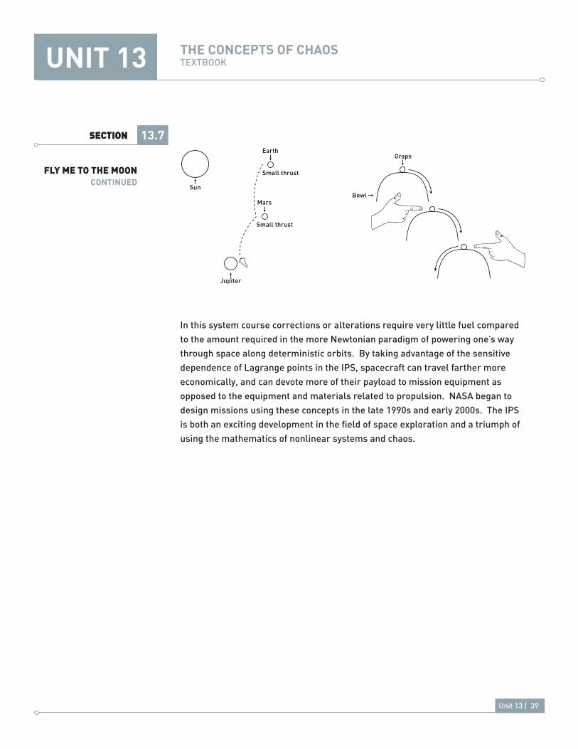
Just a minimal applied force is enough to send an object hurtling away from the Lagrange point in much the same way that a mere touch is sufficient to send a delicately balanced grape rolling off of the top of an upside-down bowl. If you knew exactly how and where to nudge the grape, you could control where it ends up (for a perfectly spherical grape). Furthermore, your small exertion would result in a large effect on the grape’s position. This is the essence of how sensitive dependence can be harnessed and used to help us explore our solar system.

Objects can sit at Lagrange points, albeit tentatively. They can also orbit them in a manner similar to how they would orbit a planet, except that orbits around Lagrange points are extremely unstable. The IPS is a very precise path that connects the different Lagrange points across our solar system. It can be visualized as a system of tubes whose surfaces represent paths that naturally tend toward Lagrange points. By staying on the surface of one of these tubes, a spacecraft can basically surf the gravitational landscape of the solar system using very little fuel. Imagine our grape being nudged off of the first overturned bowl and onto the pinnacle of another overturned bowl, where the process is repeated—a theoretically perpetual system of motion with very little input energy.

13.7

FLY ME TO ThE MOONCOnTinUED1770

A small nudge sendsa satellite away from

a Lagrange point.

A grape balances on thebowl, but a small nudge

results in a large change.

Grape

Earth

Lagrange point

Sun

Unit 13 | 39


13.1SECTION

Unit 13 | 39

SECTION

In this system course corrections or alterations require very little fuel compared to the amount required in the more Newtonian paradigm of powering one’s way through space along deterministic orbits. By taking advantage of the sensitive dependence of Lagrange points in the IPS, spacecraft can travel farther more economically, and can devote more of their payload to mission equipment as opposed to the equipment and materials related to propulsion. NASA began to design missions using these concepts in the late 1990s and early 2000s. The IPS is both an exciting development in the field of space exploration and a triumph of using the mathematics of nonlinear systems and chaos.

13.7


1770

Grape

BowlSun

Earth

Small thrust

Mars

Small thrust

Jupiter

Unit 13 | 40

UniT 13

13.1SECTION

AT A GLAnCETEXTBOOK

SECTION

Chaos is one of many behaviors that a nonlinear system can display.• A mass on a spring is an example of a simple harmonic oscillator, a well-• understood linear system.Linear systems can be solved relatively simply because they can be broken • down into parts that can be solved separately.Linear systems tend toward one of four predictable behaviors.• A pendulum swinging outside of the small-angle approximation, where • sin θ ∼ θ, is an example of a nonlinear system.For small swings, a pendulum behaves predictably, but for large swings, it • can behave strangely.

Newton calculated the motion of the planets using differential equations for • two objects influencing each other with gravity.Given the initial conditions and the relevant equations, one can predict • where the two mutually orbiting objects will be at any point in time.The three-body problem is very different from the two-body problem.• Poincaré showed that the behavior of a three-body system cannot be • quantitatively predicted.A phase portrait is a way to visualize all states of a system.• Using a phase portrait, one can deduce the qualitative features of a system’s • evolution.If a system starts out at an equilibrium point, it will not be driven to change • its state.Equilibria can be stable (attractors) or unstable (repellers).•

3.2

LIMITS OF PREDICTABILITY

13.3SECTION

13.2


Unit 13 | 41

UniT 13

SECTION

Lorenz discovered that a small change in the input to a certain system of • equations resulted in a surprisingly large change in output.The phase space of the Lorenz system contains an attractor whose phase • portrait resembles a butterfly.The Lorenz attractor helps to explain how small changes in starting • conditions lead to greater changes down the line.

A simple way to see sensitive dependence is to look at discrete, iterative • processes, such as folding dough.

A bifurcation is an abrupt change in the qualitative behavior of a system.• The logistic map is a model of population growth that exhibits many different • types of behavior, depending on the value of a few constants.Above a certain parameter value, the logistic map becomes chaotic.• While the distance between successive bifurcations in the logistic map • changes, the ratio of those distances is a constant.

Deterministic, Newtonian, mechanics were sufficient to get us to the moon • during the space race.Space scientists are able to use sensitive dependence to their advantage to • plan minimal-fuel routes through the solar system.By connecting Lagrange points, scientists have created an Interplanetary • Superhighway.

AT A GLAnCE TEXTBOOK

3.2

3.2

3.2

ThE LOgISTIC MAP

FLY ME TO ThE MOON

ITERATION

13.6

13.7

13.5

SECTION

SECTION

SECTION

13.4


Unit 13 | 42


http://ecommons.library.cornell.edu/handle/1813/97

Belbruno, Edward. Fly Me to the Moon: An Insider’s Guide to the New Science of Space Travel. Princeton, NJ: Princeton University Press, 2007.

Chernikov, Aleksander A.; Roald Z. Sagdeev, and Georgii M. Zaslavskii.“Chaos - How Regular Can it Be?” Physics Today, vol. 41, (November 1988).

Diacu, Florin and Philip Holmes. Celestial Encounters: The Origins of Chaos and Stability. Princeton, NJ: Princeton University Press, 1996.

Glass, Leon, Michael R. Guevara, Alvin Shrier, and Rafael Perez.“Bifurcation and Chaos in a Periodically Stimulated Cardiac Oscillator,” Physica, vol. 7, (1983).

Gleick, James. Chaos: Making a New Science. New York: Penguin Books, 1988.

Holland, John H. Emergence: From Chaos to Order. Reading, MA: Helix Books (Addison-Wesley Press), 1998.

Lo, M.W. “The Interplanetary Superhighway and the Origins Program” IEEE Aerospace Conference Proceedings, vol. 7, (2002).

Nolasco, J.B. and R.W. Dahlen. “A Graphic Method for the Study of Alternation in Cardiac Action Potentials,” Journal of Applied Physiology, vol. 25, no. 2 (1968).

Pikovsky, Arkady, Michael Rosenblum, and Jurgen Kurths. Synchronization : A Universal Concept in Nonlinear Sciences. Cambridge, New York: Cambridge University Press, 2001.

Smith, Douglas L. “Next Exit 0.5 Million Kilometers,” Engineering and Science, vol. 65, no. 4 (2002).

Stewart, Ian. From Here to Infinity: A Guide to Today’s Mathematics. Oxford, Great Britain: Oxford University Press, 1996.

BIBLIOgRAPhY

WEBSITES

PRINT

Unit 13 | 43


Strogatz, Steven. Nonlinear Dynamics and Chaos: With Applications to Physics, Biology, Chemistry and Engineering. Cambridge, MA: Perseus Books Publishing, 2000.

Thornton, Marion. Classical Dynamics of Particles and Systems, 4th ed. Orlando, FL: Saunders College Publishing (Harcourt Brace College Publishers), 1995.

Wang, Q.D. “Power Series Solutions and Integral Manifold of the N-Body Problem,” Regular and Chaotic Dynamics, vol. 6, no. 4 (2001).

Feynman, Richard. The Character of Physical Law. New York: Modern Library: 1994; p 108.

Poincaré, Henri (edited and introduced by Daniel L. Goroff) New Methods of Celestial Mechanics, vol. 1; Los Angeles, CA: American Institute of Physics: 1993; pp 110-111.

BIBLIOgRAPhY

PRINTCOnTinUED

Unit 13 | 44


13.1SECTIONNOTES

textbook - learner of chaos theory. imagine that two leaves, identical in every ... the position of...

Documents