textbook - annenberg learner

TEXTBOOK

UniT 2

COmBinaTOriCs COUnTsTEXTBOOK

UniT OBJECTiVEs

Combinatorics is about organization. •

Many combinatorial problems involve ways to enumerate, or count, various things • in an efficient manner.

The counting function • C(n,k), is a powerful tool used to count subsets of a larger set, or give coefficients in binomial expansions.

Bijection—the identification of a “one-to-one” correspondence—enables us to • enumerate a set that may be difficult to count in terms of another set that is more easily counted.

Pascal’s Triangle is an elegant illustration of the counting function • C(n,k).

Techniques from graph theory can help with combinatorial challenges such as • finding circular permutations.

The pigeonhole principle—the idea that if you have more pigeons than holes, some • holes must have more than one pigeo—is a deceptively simple idea that can be used to prove startling results.

Ramsey Theory explains why we sometimes find order in supposed randomness. •

Ideas from combinatorics are at play in modern methods of DNA sequencing. •

The question of whether or not P = NP—whether certain types of seemingly • computationally intractable combinatorial problems can be solved in reasonable amounts of time—is at the forefront of current research in both combinatorics and computer science.

UniT 02

mathematics may be defined as the economy of counting. There is no problem in the whole of mathematics which cannot be solved by direct counting.

E. MACh

Unit 2 | 1

UniT 2 COmBinaTOriCs COUnTs TEXTBOOK

2.1SECTIONDNA is the genetic information that encodes the proteins that make up living things. human DNA is a large molecular chain consisting of sequences of four different building blocks known as nucleotides. These nucleotides, adenine, cytosine, guanine, and thymine, combine to form the different genes that make us who we are. human DNA consists of about 3 billion pairs of these building blocks.

In 1990, the U.S. Department of Energy, in conjunction with the National Institutes of health and an international consortium of geneticists from China, France, Germany, Japan, and the UK, set out to map the entire sequence of base pairs in human DNA. The human Genome Project, as it was called, was projected to take fifteen years to complete. By the year 2000, just ten years later, a rough draft was announced and by 2003, the sequence was declared to be essentially complete, two years ahead of schedule.

What enabled this huge project to be completed more quickly than expected? There were many factors, most significantly improvements in technology and faster computers, which made it possible to complete time-consuming calculations within more reasonable time frames. This new generation of computers made it realistic to run powerful algorithms from the mathematics of organization, combinatorics. Combinatorics is, simply put, the mathematics of counting things—things that are generally collections of mathematically defined or encoded objects. As such, combinatorics is the branch of mathematics that is central to some basic problems inherent in our data-rich age: the organization of large sets of data and the quest to uncover relational meaning among the members of those sets. For example, when faced with a task of, say, combining “puzzle pieces” of DNA to make a complete model, combinatorics can be used to enumerate the possibilities. Not only does this tell us whether our ordering is feasible, it also provides the tools that actually accomplish this ordering.

As we already noted, the effort to determine the human genome is a modern context for applying combinatorics. A more classic problem is the infamous “traveling salesperson problem:” Suppose that you are a traveling salesperson and you wish to find the shortest route connecting a group of designated cities. A simple combinatorics problem will help you establish the number of possible itineraries. however, it turns out that finding the shortest possible route, for even a relatively small number of cities, is much more difficult—in fact, it may even be computationally intractable. These are all problems of combinatorics.

INTRODUCTION

Unit 2 | 2


2.1SECTIONNot only can combinatorics help to organize complicated sets, but it can also reveal whether or not any organization inherently exists in large, seemingly “random” sets. This idea, known as Ramsey theory, gives some quantitative rationale as to why we see constellations in the night sky. It also explains, and debunks, some claims of the existence of hidden messages in the Bible. Ramsey theory shows mathematically that structure must exist in randomness, although it does not provide any guidance or formula for finding such structure.

In this unit, we will look at some of the uses of combinatorics, such as finding combinations and permutations and sequencing DNA. We will also learn about the general techniques of the combinatorialist, from bijection, to the “pigeonhole principle,” to uses of hamiltonian cycles in connected graphs. We will also explore a bit of the history of this incredibly useful field, from the counting problems of ancient Egypt, to the mysterious triangle of Pascal, to questions at the forefront of modern-day computing.

INTRODUCTIONCOnTinUED

Unit 2 | 3


SECTION

The Rhind Papyrus• Flavors in India• Functions•

Bijective Proof•

ThE rhinD PaPyrUs

The Rhind Papyrus, also known as the Ahmes Scroll, is the earliest known • combinatorial problem.The solution to the problem requires using the sum of a geometric series.•

The problem of keeping track of large numbers of possibilities is by no means a new one. The mathematicians of the middle kingdom in Egypt were quite aware of how quickly such problems can grow. An early piece of evidence of this comes from the Rhind Papyrus. This scroll, transcribed by Ahmes from Egyptian 12th Dynasty mathematical texts, contains problems illustrating many different mathematical concepts, usually presented in applied form. One such problem, “Number 79,” sometimes referred to as “the Inventory Problem,” lays out a not-so-straightforward counting scenario:

There are seven houses; in each house there are seven cats; each cat kills seven mice; each mouse has eaten seven grains of barley; and each grain would have produced seven hekats (an old unit of measure equivalent to about 5 liters). What is the sum of all the enumerated things?

EgypT aND INDIa

2.2

Item 1040 / Egyptian, RhIND MAThEMATICAL PAPYRUS COPIED BY ThE SCRIBE AhMES (ca. 1650 BCE). Courtesy of Art Resources, Inc.

Unit 2 | 4


SECTION

We can approach this problem, as the Egyptians did, in a so-called “brute force” fashion, by multiplying and adding four consecutive times. If there are seven houses, each of which has seven cats, then there is a total of forty-nine cats. The fact that there were seven mice munched by each cat means that a total of 343 mice met their demise. Continuing in this manner, we calculate that 2,401 grains of barley were eaten along with the mice, thereby keeping 16,807 hekats of barley out of production. Adding together all the quantities involved (i.e., houses, cats, mice, barley grains, and hekats of barley), we find that there were 19,607 things in total.

Notice that this problem involves finding the sum of a sequence of terms that increase geometrically—that is, each term is a constant multiple of the previous

EgypT aND INDIaCOnTinUED

2.2DIAGRAM OF A BRANCHING TREE

Item Quantity SubtotalHouses 7 7Cats 49 56Mice 343 399Barley (spelt) 2401 2800Hekats 16,807 19,607total 19,607 19,607

1132

RHIND PAPYRUS PROBLEM

Unit 2 | 5


SECTION 2.2 one. Starting with seven, and multiplying by seven each time, we get to almost 17,000 in four steps. This is an example of a geometric series, and it shows how quickly such a series can grow. We can find the desired sum in this case by adding the first five powers of seven:

71 + 72 + 73 + 74 + 75 = 7 + 49 + 343 + 2,401 + 16,807 = 19,607

More generally, a geometric series is the sum of a sequence of terms in which each new term is generated by multiplying the preceding term by some fixed common factor. For example, the finite geometric series 1 + 2 + 4 + 8 +...+2n (for some value of n) is such that each term is two times the term that precedes it. A famous illustration of the speed at which such a series grows is the one that asks how much money it would take to place one penny in the first square of a chessboard, two pennies in the second square, four in the third square, eight in the fourth square, and so on until there is a stack of pennies in each of the board’s sixty-four squares. Fortunately, we do not have to use brute force, as the Egyptians would have, to solve this. The clever solution goes like this:

In general, we can express a geometric series in this form:

a + ar + ar2 + ar3 + ar4 + … + arn

where a is some initial value and r is the constant factor or ratio. The general

solution, then, of the sum of this geometric series is S = a (rn+1-1)

(r-1).

In the case of the pennies piling up on the chessboard, a = 1 and r = 2. Because there are sixty-four squares on a chessboard, n = 63 (the first square has one

penny, represented by 20). The sum is, therefore,

1 (263+1 - 1)

(2 - 1), which is equal to

about 1019 pennies, or 1017 dollars (in non-scientific language, that’s 100 million billion dollars)! This powerful example of how quickly a geometric series expands gives us a glimpse of the magnitude of combinatorial explosions.

Using a formula to find the sum of the geometric series underlying the Egyptian “inventory problem” and the pennies on the chessboard example demonstrates an important idea underlying combinatorial mathematics—problems in which the work grows very rapidly can often be reduced in clever ways to problems that are more easily controlled. This idea popped up again in India in the 7th century AD, this time having to do with combinations of flavors.


Unit 2 | 6


SECTIONFlaVOrs in inDia

The problem of counting subsets of a larger set was explored by thinkers in • India as early as the 6th century BC.

The Indian medical text, Sushruta Samhita, written by Sushruta in the 6th century BC, examines the ways in which six fundamental flavors, bitter, sour, salty, sweet, astringent, and hot, could be combined. (Note: It is important to realize that for the purposes of this discussion, by “combinations,” we mean subsets of a larger set in which order doesn’t matter; salty-sweet is the same as sweet-salty.) This ancient text showed that there were sixty-three such combinations, categorized as follows: six single tastes, fifteen pairs, twenty triples, fifteen quadruples, six quintuples, and, of course, one combination of all six tastes. There is, incidentally, one way to have zero flavors, generally called the “empty set,” but we will disregard this because “flavorless” doesn’t count as a flavor. Adding all of these possible groupings together, we can easily see that their sum is sixty-three, but is there a more clever and basic way to look at this?

One way to approach this problem would be to make an organized list. We could represent the six flavors with the letters A, B, C, D, E, and F and begin by listing the possible “combinations” of one: A, B, C, D, E, F. Then we can list the possible pairs: AB, AC, AD, AE, AF, BC, BD, BE, BF, CD, and so on. There seems to be a more general idea at work here. Can we get to it?

2.2


1133

AB AC AD AE AFBC BD BE BF CDCE CF DE DF EF

ABC ABD ABE ABF ACDACE ACF ADE ADF AEFBCD BCE BCF BDE BDFBEF CDE CDF CEF DEF

ABCD ABCE ABCF ABDE ABDFABEF ACDE ACDF ACEF ADEFBCDE BCDF BCEF BDEF CDEF

A B C D E F

ABCDE ABCDF ABCEF ABDEF ACDEF BCDEF

ABCDEF

ORDERED LIST

Unit 2 | 7


SECTION 2.2FUnCTiOns

Functions map members of one set to members of another set.•

To help us reach an efficient solution to “the problem of the flavors,” we can look for some function that will enable us to count the number of subsets of a given set of size n quickly and conveniently. Generally, we think of functions as math machines into which we put numbers and which spit out correlated numbers, but we can also think of a function as a way to describe how one set relates to another. In this set-based concept, a function is a rule that assigns to each member of a set of input values one, and only one, output value. For example, the absolute value function, |n|, takes all real numbers as inputs and maps each of them to their distance from the origin. Because distance is measured as a non-negative value, the function |n| maps the set of all real numbers to the set of non-negative real numbers. The inputs “5” and “-5” get assigned the same output of “5.”

BiJECTiVE PrOOF Bijection can be used to enumerate the members of a difficult-to-enumerate • set by establishing a one-to-one correspondence with a set that is easier to enumerate. Using the concept of bijection, we can solve the Indian flavors problem in a • very elegant way.

The concept that no single input gives more than one output is common to all simple functions. Some functions, however, are more restrictive. In addition to restricting each input to only one output, these functions require that each output is matched with exactly one input. Such functions, which are called “bijections” or “one-to-one correspondences,” can be quite useful to us as we attempt to find clever solutions to combinatorial problems. To do so, we seek to show that two sets (the one that we are trying to find and another that

2124-55

3

7

-3

-7

5

3

7

-5-3-7

53

7

TWO VIEWS OF THE ABSOLUTE VALUE FUNCTION

n


Unit 2 | 8


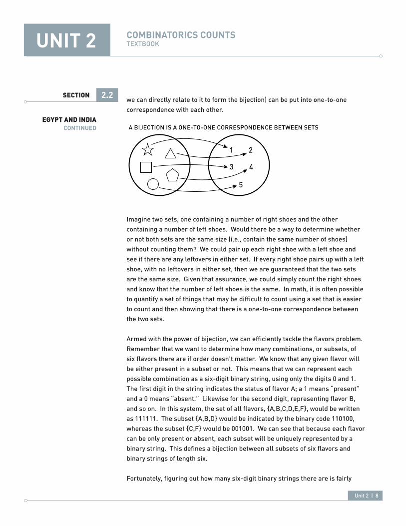
SECTIONwe can directly relate to it to form the bijection) can be put into one-to-one correspondence with each other.

Imagine two sets, one containing a number of right shoes and the other containing a number of left shoes. Would there be a way to determine whether or not both sets are the same size (i.e., contain the same number of shoes) without counting them? We could pair up each right shoe with a left shoe and see if there are any leftovers in either set. If every right shoe pairs up with a left shoe, with no leftovers in either set, then we are guaranteed that the two sets are the same size. Given that assurance, we could simply count the right shoes and know that the number of left shoes is the same. In math, it is often possible to quantify a set of things that may be difficult to count using a set that is easier to count and then showing that there is a one-to-one correspondence between the two sets.

Armed with the power of bijection, we can efficiently tackle the flavors problem. Remember that we want to determine how many combinations, or subsets, of six flavors there are if order doesn’t matter. We know that any given flavor will be either present in a subset or not. This means that we can represent each possible combination as a six-digit binary string, using only the digits 0 and 1. The first digit in the string indicates the status of flavor A; a 1 means “present” and a 0 means “absent.” Likewise for the second digit, representing flavor B, and so on. In this system, the set of all flavors, {A,B,C,D,E,F}, would be written as 111111. The subset {A,B,D} would be indicated by the binary code 110100, whereas the subset {C,F} would be 001001. We can see that because each flavor can be only present or absent, each subset will be uniquely represented by a binary string. This defines a bijection between all subsets of six flavors and binary strings of length six.

Fortunately, figuring out how many six-digit binary strings there are is fairly

2.2


21191 2

3 4

5

A BIJECTION IS A ONE-TO-ONE CORRESPONDENCE BETWEEN SETS

Unit 2 | 9


SECTIONstraightforward and much easier than counting subsets of flavors. Each digit has only two options; it must be a 0 or a 1. We can simply multiply the number of options for each digit to figure out how many possible strings there can be.

2 × 2 × 2 × 2 × 2 × 2 = 26 = 64 strings

One of those strings, 000000, corresponds to “no flavor,” however, and we have already decided to disregard that option, so we end up with a grand total of sixty-three subsets. In general, we have found that the number of non-empty subsets of n elements is 2n-1. This method is significantly faster than listing all the possible combinations. The drawback of this method is that it does not tell us how many subsets of a given size there are.

Recall that, according to the Indian text, there are six single flavors, fifteen pairs, twenty triples, fifteen quadruples, six quintuples, and one way to combine all six flavors. Is there a way to find these numbers—to enumerate subsets according to their size—without listing and sorting all possible combinations? Our method of finding a bijection between the total number of subsets and binary strings doesn’t immediately give us this level of detail. In the next section we will see how to count subsets of a particular size by using a function that has many uses in both combinatorics and beyond, C(n,k).

2.2


Unit 2 | 10


SECTION 2.3

Permutations• From Permutations to Combinations •

PErmUTaTiOns Counting combinations, in which order does not matter, is different than • counting permutations, in which order does matter.The factorial operation is very important in counting permutations.•

We can solve the problem of the flavors by a different method that will give us a broader understanding of the subsets than the bijection method provided. Specifically, we need a strategy that not only reveals the total number of subsets, but that is also capable of categorizing the subsets by size. This is a common theme in mathematics; solving problems in different ways deepens our understanding of what is really happening. To re-phrase our problem, we are seeking a formula that will tell us how many subsets of a given size can be made from the original set of six flavors. We would then like to generalize this formula to tell us how many subsets of size k, called k-subsets, can be made of a set of n elements. In doing this, we will have to use the important combinatorial concepts of permutation and combination.

We can start our thought process by considering how many ways the six flavors can be arranged if we count each unique ordering separately. (Remember that previously we gave no significance to order and considered, for example, the subsets AB and BA to be the same.) Arrangements such as these, in which order matters, are known as permutations. We can imagine the possible permutations of six flavors as a sequence of six empty slots.

Notice that there are six possible flavors that can occupy the first slot, five that can occupy the second, four for the third, and so on. This is because once a

FlavORS REvISITED

3071ABCDEF

BCDEF

CDEF

DEF

EF

F

POSSIBILE CHOICES FOR SLOTS

Unit 2 | 11


SECTION 2.3 specific flavor is used, we don’t want it to appear again in the same permutation. The total number of permutations of six flavors is then 6 × 5 × 4 × 3 × 2 × 1 = 720, which we denote as 6!, called “six factorial.” In general, the number of permutations of n objects will be n! As a shorthand, we can write P(n,n), or “the permutations of n objects taken n at a time.”

So, permutations have a simple formula in terms of the factorial, but there is more to consider. Remember, we also want to be able to find the number of arrangements involving fewer than all six of the elements—what we call subsets. Furthermore, in the final analysis we are not concerned with the order of flavors; we really don’t care if a subset has salty before sweet or sweet before salty. Such arrangements, in which order does not matter, are known as combinations. To find a formula for counting combinations of a given size, we will have to deal with both of these considerations.

First, let’s figure out how to deal with finding smaller arrangements selected from a pool of six objects in which order still matters. For example, to find the number of ways to order two flavors out of the set of six, we can imagine two slots, the first of which has six possible flavors, the second of which has only five possible flavors, once a flavor has “filled” the first slot. After multiplying, as we did before, we see that there are thirty possible ways to order two out of the six flavors. In the language of combinatorics, we say that we have found the number of permutations of six objects taken two at a time. We can write P(6,2) to express this; the general form for this expression is P(n,k), or “the permutations of n objects taken k at a time.”

Notice that P(6,2) is less than P(6,6). Why is this? P(6,6) gives the total number of unique orderings of all six flavors, but to find P(6,2), we are concerned with only two flavors. Going back to the six–slot concept from before, we can let the two flavors we care about occupy the first two slots. For example:

A B _ _ _ _

The remaining four slots can be ordered in 4! (24) ways, all of which have the same first two flavors. So, P(6,6) over-counts P(6,2) by a factor of twenty-four. Therefore, to find P(6,2), we should divide P(6,6) by 4!. Recognizing that 4 = (6-2), we can write the following expression for the value of P(6,2):

P(6,2) =

6!

(6 − 2)!

FlavORS REvISITED COnTinUED

Unit 2 | 12


SECTIONWe can then generalize this for P(n,k):

P(n,k) =

n!

(n −k)!

This is the formula for the number of permutations of n objects taken k at a time.

FrOm PErmUTaTiOns TO COmBinaTiOns

The formula for combinations of n objects taken k at a time can be found • by first looking at the permutations of n objects taken k at a time and then dividing by the number of permutations of k objects taken k at a time.

having addressed the first of our concerns—counting smaller permutations—we can move on to the question of what to do about order. Permutations, recall, count each unique ordering of objects separately, but in the problem of the flavors, we don’t really care about the order of flavors in a subset. Knowing that P(n,k) gives the number of permutations of n objects taken k at a time, can we use this to determine the number of combinations in a subset of permutations? If so, we could then find the number of combinations of six, five, four, three, two, and single flavors. Then, after adding these together, we will have found the total number of subsets of six flavors.

We can start by realizing that the number of permutations will always be greater than the number of combinations. For example, P(n,k) treats the arrangements ABC, ACB, BCA, BAC, CAB, and CBA as different. Viewing them as combinations of three flavors, however, we would consider them all to be the same combination. So, P(n,k) must be over-counting if we are interested only in combinations. By what factor does P(n,k) over-count?

P(n,k) over-counts by the number of ways to arrange k objects. This is evident in the example of six permutations of three objects taken three at a time above. If we divide the six objects by 3!, or six, we get one, which is the number of combinations of three objects, taken three at a time. In general,

P(n,k)

P(k,k)will tell

us the number of combinations of n objects taken k at a time. We call this C(n,k). Using the formula for P(n,k) from above and recognizing that P(k,k) = k!, we can write:

C(n,k) =

n!

k!(n −k)!

2.3


Unit 2 | 13


SECTIONFor example, C(10,3) represents the number of possible three-topping pizzas that we could choose given a total of ten possible toppings.

Using this notation, we can complete the following short chart to solve the original problem of the flavors by enumerating the subsets according to their size.

Adding the results for the number of subsets of size one, two, three, four, five, and six elements, we get:

6 + 15 + 20 + 15 + 6 + 1 = 63

Although it took us a while to derive the formula for C(n,k), using it to count k-subsets in this manner is much faster than listing them all.

We have now efficiently answered the problem of the flavors in two different ways, and we can see that adding together all the possible values of C(n,k), as k ranges from 1 through 6, yields the same value that we found in our previous solution using bijection. Furthermore, we can imagine that each of the specific k-subsets corresponds to a unique binary string. In our next section, we will use a similar method to derive what is going on at the heart of one of the most famous and fascinating number patterns in mathematics: Pascal’s Triangle.

2.3


3072

= number of unordered subsets

C(6,1) = 6 sets of 1

C(6,2) = 15 sets of 2

C(6,3) = 20 sets of 3

C(6,4) = 15 sets of 4

C(6,5) = 6 sets of 5

C(6,6) =1 set of 6

VALUES OF THE COUNTING FUNCTION

6!1!(5!)

6!2!(4!)

6!3!(3!)

6!5!(1!)

6!4!(2!)

6!6!

N!k!(n −k)!

Unit 2 | 14


SECTION

Find the Weirdo• The Triangle Takes Shape •

FinD ThE WEirDO

Pascal’s Triangle is an important and widely useful mathematical concept.• At its heart, Pascal’s Triangle is a recursive relationship by which we can, • given previous elements, find subsequent ones.

The counting function C(n,k) and the concept of bijection coalesce in one of the most studied mathematical concepts, Pascal’s Triangle. At its heart, Pascal’s Triangle represents a recursive way to compute all the C(n,k), the numbers of k-subsets of an n-element set for any n and any k. As a recursive pattern, Pascal’s Triangle incorporates previously known values in the creation of new ones. To portray the relationship at the heart of the triangle, we will again solve a particular problem in two different ways.

Once again let’s address the question of how many k-subsets there are of an n-element set. Solved one way, we know the answer is

n!

k!(n −k)! . Now as we explore the question again, we will also consider whether or not a k-subset contains the element “n”. Using the flavors example, we would sort all of our combinations of flavors into two sets, those that have “salty” as one of their components and those that do not. In this strategy, sometimes known as “weirdo” analysis; we call “n” or “salty” the “weirdo” and make deductions by counting the sets that either contain it or don’t contain it.

To start, let’s focus on just the k-subsets. We can separate these subsets into two piles. Pile A will have all the k-subsets that contain the element n. Pile B will have all the k-subsets that do not contain n. In terms of flavors, A has all of the combinations containing “salty,” and B has all those that don’t. Note that both pile A and pile B are sets of subsets.

All of the subsets in pile A have to contain n; therefore, to figure out how many of them there are, we can just pretend that they are only of size k-1 (because one of the slots is always filled by n).

_ _ _ _ … n

2.4

paSCal’S TRIaNglE

Unit 2 | 15


SECTION 2.4 (In other words, k spaces, one of which is always filled by n, means that there are actually only k-1 spaces in play.)

Likewise, because n is not allowed to move around, it is in some sense “out of play” in our larger n-sized set. This means that each of the subsets in pile A has k-1 spaces to fill using only the elements {1, 2, …, n-1}. The number of these subsets in pile A is the same as the number of k-1 subsets of an (n-1)-sized set. We thus have a bijection between the set of k-sized subsets containing n and the set of (k-1)-sized subsets of an (n-1)-sized set.

We know the way to find how many (k-1)-sized subsets there are of (n-1) by using our C(n,k) formula. For simplicity’s sake we’ll just write C(n-1,k-1).

Now, let’s look at pile B containing the k-sized subsets that do not contain n. For each subset we have to fill k spaces using only the elements {1, 2, …, n-1}. This is the same as asking how many k-sized subsets there are of an (n-1)-sized set. We again can use our handy formula, written as C(n-1,k).

Finally, we know that if we combine pile A and pile B, we should have the total amount of k-sized subsets of an n-sized set, which can be expressed as C(n,k).

The total number of subsets of size k, C(n,k), is equal to the total of those that include n, the weirdo, C(n-1, k-1), plus those that don’t, C(n-1, k), or:

C(n,k) = C(n-1, k-1) + C(n-1,k)

This relationship, known as Pascal’s equation, gives us a recursive relationship that enables us to compute the number of k-subsets of an n-element set using the results we already have for smaller subsets of smaller sets. Organizing the results of a few iterations of this rule into a chart yields an interesting structure.

paSCal’S TRIaNglECOnTinUED

2126 + = C(n,k)A B

PILE A + PILE B = SUBSETS OF N

Unit 2 | 16


SECTIONThE TrianglE TaKEs shaPE

Pascal’s equation can be used to create his famous triangle, which can in • turn be used in a variety of ways to count different types of subsets.There are many interesting mathematical relationships, or identities, hidden • within Pascal’s Triangle.

Looking at a few iterations of Pascal’s equation gives us the following result in tabular form:

This information is probably more familiar to you presented in the following form:

In this arrangement, each number is denoted by C(row, column). Note that the first row is considered row zero, as is the first column. So, returning to our taste example, we can find the number of combinations of three out of six by looking at row 6 and finding column 3. The value found in that position, 20, is in complete agreement with everything we’ve done before. To find how many subsets of any size there are in a group of six, we simply add all the numbers in the sixth row, taking care not to add the 1 that represents the empty set.

Notice that C(0,0) and C(n,n) are both equivalent to one, reminding us that there

2.4


1139

1

20

11

15

11

61

11

11 2

15

1 3 3

51 4 6 4

61 10 10 5

35 21 7352171

1

STANDARD DIAGRAM OF PASCAL’S TRIANGLE THROUGH SEVENTH ROW

1138

K

n

0 1 2 3 4 5 6 70 C(0,0) = 11 C(1,0) = 1 C(1,1) = 12 C(2,0) = 1 C(2,1) = 2 13 1 3 3 14 1 4 6 4 15 1 5 10 10 5 16 1 6 15 20 15 6 17 1 7 21 35 35 21 7 1

PASCAL’S TRIANGLE

Unit 2 | 17


SECTIONis only one way to choose zero items out of a set of zero, and only one way to choose n items out of a set of n items when the order does not matter.

Pascal’s Triangle is a mathematical paradise, with many interesting relationships hidden in its structure. First, note that the sum of entries of any row n is equal to 2n, in agreement with our binary strings bijection from before.

4th ROW1 + 4 + 6 + 4 + 1 = 162n = 24 = 16

Also, the entries in the nth row of the triangle give the coefficients of the terms in the expansion of a simple binomial raised to the power n, such as (x+y)n. For example:

(x+y)3 = 1x3 + 3x2y + 3xy2 + 1y3

The coefficients of this polynomial can be found in the third row of Pascal’s Triangle. Because they are useful in expanding binomials, the various sets of C(n,k)s are also known as binomial coefficients. Note that this isn’t magic; it’s simply the result of counting the number of subsets with k factors of x.

Another interesting phenomenon in Pascal’s Triangle can be found by looking at so-called “hockey-sticks.” A hockey-stick is a pattern within the triangle composed of a diagonal string of numbers and a terminating offset number, such as those shown here:

2.4


Unit 2 | 18


SECTION 2.4

What is fascinating in a hockey-stick pattern is that the linear string of numbers, when added together, totals the value of the number that is offset. For example, the sum of the numbers 1, 6, 21, and 56 is 84 (the blue pattern in the figure above). This works no matter where in the triangle we draw a hockey stick, as long as it starts with a “1.”

To get a sense for why this holds true, let’s look at the orange hockey stick above, 1 + 3 + 6 = 10. Recognizing the “10” in our pattern as the second entry of the 5th row, we can write it as 10 = C(5,2). Let’s plug this into Pascal’s equation:

C(n,k) = C(n-1, k-1) + C(n-1, k)

C(5,2) = C(4, 1) + C(4, 2)

Note that C(4,2) is the second entry in row four, “6,” which is part of our hockey stick. however, C(4,1), the first entry in row four, is not part of our pattern. If we use Pascal’s equation again, we find:


3087

1

1

1

1

1

1

1

1

1

1

1

1

1

1

2

3

4

3

5

6

7

8

9

10

11

12

13

6

10

15

21

28

36

45

55

66

78

4

10

20

35

56

84

120

165

220

186

1

1

1

1

1

1

1

1

1

1

1

1

1

5

6

7

8

9

10

11

12

13

15

21

28

36

45

55

66

78

35

56

84

120

165

220

186

70

126

210

330

495

715

126

252

462

792

1287

210

462

924

1716

495

1287715

330

792

1716

HOCKEY STICKS IN PASCAL’S TRIANGLE

Unit 2 | 19


SECTIONC(4,1) = C(3, 0) + C(3, 1)

C(3,0) = 1 and C(3,1) is the first entry of row three, which is “3.” Plugging these results back into the equation for C(5,2), we get:

C(5,2) = C(4,2) + C(3,1) + C(3,0) => 10 = 6 + 3 + 1

This is the hockey stick identity that we set out to prove!

There are many other fascinating mathematical series and relationships to be found in the triangle, such as triangular numbers, primes and their multiples, and Fibonacci numbers to name but a few.

By the way, Pascal did not invent this triangle. It was known centuries earlier to both the Indians and Chinese as having particular use in finding combinations, as we have just seen. The Chinese mathematicians Yang hui and Chu Shih Chieh knew about it at least 350 years before Pascal’s work.

2.4


Unit 2 | 20


SECTION

Circular Ordered Selections• A Royal Problem• Enter Graph Theory •

CirCUlar OrDErED sElECTiOns Counting permutations is different than simply counting combinations • because order must be taken into account.

So far we have learned how to consider both ordered and unordered subsets. how might our results change if we require that the arrangements be circular? To put this into context, let’s phrase all our previous problems in terms of dinner parties. In this scenario n! is the number of ways of putting n people along one side of a banquet table. C(n,k) is the number of ways of choosing k people out of n to sit together at a table. What if we have circular tables, however, and we want to count the number of ways that a given number of people can be arranged around one of these?

Suppose we are expecting ten people for dinner; how many ways can we seat them around a circular table? First, let’s think about how many ways we can line them up. As we indicated above, there will be 10! ways to line up ten guests: ten for the first position, nine for the second, eight for the third, and so on.

how does this change if they are seated around a circular table? Concepts such as this are called circular permutations, and they are not exactly like linear permutations.

2.5

ThE ORDER OF ThE gaRTER

2128

10 PEOPLE LINED UP

Unit 2 | 21


SECTION

Notice that every circular arrangement corresponds to ten different linear arrangements.

Using our reasoning from before, we can see that the number of circular arrangements is equal to the number of linear arrangements, 10!, divided by ten to compensate for the fact that each circular permutation corresponds to ten different linear ones. This gives as the number of ways to arrange

2.5


COnTinUED

2129

1

6

2

3

4

57

8

9

107

2

8

9

10

13

4

5

6

THESE CIRCULAR PERMUTATIONS ARE EQUIVALENT

2130

1

6

2

3

4

57

8

9

10

1 2 3 4 5 6 7 8 9 10

2 3 4 5 6 7 8 9 10 1

3 4 5 6 7 8 9 10 1 2

4 5 6 7 8 9 10 1 2 3

5 6 7 8 9 10 1 2 3 4

6 7 8 9 10 1 2 3 4 5

7 8 9 10 1 2 3 4 5 6

8 9 10 1 2 3 4 5 6 7

9 10 1 2 3 4 5 6 7 8

10 1 2 3 4 5 6 7 8 9

ONE CIRCULAR PERMUTATION EQUIVALENT TO TEN LINEAR ONES

9! = 10! –––– 10!

Unit 2 | 22


SECTIONten guests around a table. We can generalize this to say that n elements can be arranged in (n-1)! ways around a circle.

a rOyal PrOBlEmThe seating arrangement at the annual brunch of the Order of the Garter in • England is an example of circular permutations in action.

It may seem to you that problems such as these are just more examples of mathematicians’ hypothetical word problems, but this problem of circular arrangement pops up yearly in England. Every year in June, a procession and service take place at Windsor Castle for the Order of the Garter—England’s oldest order of chivalry (founded by Edward III in 1348.) Following the installation of new members in the Throne Room, the Queen of England and Duke of Edinburgh host a luncheon for members and officers of the Order in Waterloo Chamber. Tradition holds that seating charts for the luncheon are rotated so that no two guests will have sat next to one another in the last ten years.

With forty-five people to consider, this problem could pose quite a headache if we attacked it with the brute force method. If order matters, there are 44! possible arrangements, which is about 1054. Checking just one of these arrangements per second would take 1046 years, which is about thirty-six orders of magnitude longer than the universe has been in existence. Recall, however, that we need ten consecutive years in which nobody has sat next to the same person twice. This means that we need to check all of the subsets of ten arrangements out of a possible 44!, which is C(44!,10). This number is much larger—yet another combinatorial explosion.

EnTEr graPh ThEOry

We can envision circular permutations as hamilton cycles on complete • graphs.

Of course, using the organizing principles of combinatorics, there is a better way. We could represent the forty-five members and their connections to each other as a diagram of forty-five points, all of which are connected to one another.

Such a diagram is called a graph, with each point being a node, and each connection an edge. A graph in which every node is connected to every other node is called a complete graph. The standard notation for a complete graph

2.5


COnTinUED

Unit 2 | 23


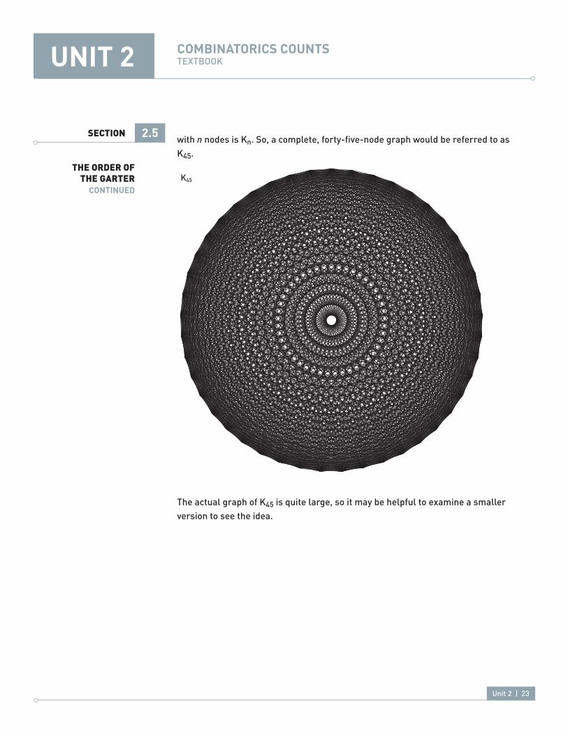
SECTIONwith n nodes is Kn. So, a complete, forty-five-node graph would be referred to as K45.

The actual graph of K45 is quite large, so it may be helpful to examine a smaller version to see the idea.

2.5


COnTinUED

3081K45

Unit 2 | 24


SECTION

If we had just five people, A, B, C, D, and E, our complete K5 graph would look like that in the diagram. We can come up with circular table arrangements of these five people by looking at paths that visit all the nodes exactly once and return to the start. Such a configuration is known as a hamilton cycle. Remember that a connection on the graph represents two people sitting next to each other. In our current problem related to seating the Order of the Garter luncheon guests we are concerned with hamilton cycles that share no common edges. Such cycles are said to be mutually disjoint. Two of these cycles for a five-person arrangement are shown in the diagram.

2.5


COnTinUED

1141A B

C

D

E

OVERLAY OF TWO CYCLES

1140Complete K5

A Hamilton cycle

Two mutually disjointHamilton cyclesAEDBCA and ADCEBA

BA

C

D

E

BA

C

D

E

A B

C

D

E

A B

C

D

E

Unit 2 | 25


SECTIONNotice that with these two cycles, every edge is accounted for. So, although we may be able to construct other cycles, they will always include at least one of the edges that we’ve already used. This means that there are two, and only two, mutually disjoint hamilton cycles for an arrangement of five elements. Consequently, we could have only two annual luncheons, at most, before two of the five people sat next to each other again.

We can see why there can be no more than two mutually disjoint arrangements in this situation by thinking about it from the perspective of one of the people seated at the table, let’s say it’s the queen. The queen will always sit next to two people, one on her right and one on her left. In the K5 case, there are only four other “non-queen” people to sit by, so the queen will have sat next to everyone after two years.

We can use similar lines of reasoning with arrangements of more people. For example, to find mutually disjoint, circular arrangements of seven or nine people, we can look at possibilities within the K7 and K9 graphs, respectively.

2.5


COnTinUED

1142

B

CA

D

EF

G

B C

E

F

G

A D

B

CA

D

EF

G

HAMILTON CYCLES ON K7

2131

K7 AND K9

Unit 2 | 26


SECTION

Notice that K7 has three mutually disjoint hamilton cycles within it and K9 has four. Applying the queen’s perspective and reasoning as we did before, we can deduce that there cannot be more than three years of non-duplicate seating for seven people and not more than four years for nine people. Extending this reasoning to the original problem, that of forty-five people, we see that the queen has forty-four possible luncheon neighbors. Taken two at a time, one on her right and one on her left, it would take her twenty-two years to sit by each one.

2.5


COnTinUED

1143

A D

E

F

G

H

I

B C

A D

E

F

G

H

I

B C

A D

E

F

G

H

I

B C

A D

E

F

G

H

I

B C

HAMILTON CYCLES ON K9

2131

K7 AND K9

2131

K7 AND K9

Unit 2 | 27


SECTIONThis means that in our banquet group of forty-five members of the Order of the Garter, there can be at most twenty-two arrangements in which no two people sit next to each other more than once. In fact, twenty-two is always attainable— more than enough for ten years’ worth of banquets. In general, the graph K2n+1 will always have n disjoint hamilton cycles incorporated within it.

Finding possible orderings of dinner guests efficiently turns out to require some quite interesting math involving graphs and circuits. These concepts are applicable in other areas as well, and they can be used to show why certain relationship structures, such as mutual friendship or mutual unfamiliarity, must exist in randomly selected groups of people. Next, we will look at Ramsey Theory and how it can be used to find organization in a number of situations.

2.5


COnTinUED

2555

THREE MUTUALLY DISJOINT HAMILTON CYCLES ON K6

Unit 2 | 28


SECTION

More Pigeons than holes• The Party Problem• Ramsey Numbers •

mOrE PigEOns Than hOlEs

Dirichlet’s box, better known as the pigeonhole principle, is a deceptively • powerful concept that can be used to prove combinatorial results.

Of central importance in Ramsey Theory, and in combinatorics in general, is the “pigeonhole principle,” also known as Dirichlet’s box. This principle simply states that we cannot fit n+1 pigeons into n pigeonholes in such a way that only one pigeon is placed in each hole, with no pigeons left over.

The pigeonhole principle may seem to be too obvious and simple to be useful. It can, however, be used to demonstrate possibly surprising results. For example, in any big city, Los Angeles let’s say, there must be at least two people with the same number of hairs on their heads. To see why this is a certainty, let’s assume that a typical person has about 150,000 hairs on his head. Let’s also assume that no one has more than a million head hairs.

There are significantly more than one million people in Los Angeles. If we consider each specific number of hairs on a head to be a pigeonhole and each

2.6

RamSEy ThEORy

2132

THE PIGEONHOLE PRINCIPLE

Unit 2 | 29


SECTIONperson to be a pigeon, then we can assign the pigeons to the holes representing the number of hairs on their heads. To summarize, there are no more than a million pigeonholes, a million distinct possible numbers of hairs on a head, and more than a million people (“pigeons”). Consequently, there will be more than one person with a given number of hairs on their heads.

We’ll see how this deceptively powerful concept plays out next in the field of Ramsey Theory.

ThE ParTy PrOBlEm

“The Party Problem” states that in any group of six people, either three • people will all know each other, or three people will not know each other.“The Party Problem” is an example of Ramsey Theory.•

Phrased another way, the Party Problem reveals that in any group of six people, we are mathematically guaranteed to find either three mutual friends or three mutual strangers. This is not true in a group of five people, so why is six the magic number?

Let’s say you attend a party and become engaged in a discussion with five other people. The six of you could be represented graphically by K6 , the complete graph on six nodes. In this discussion, the relationships between people will be represented by colored edges on the graph, with a blue edge indicating that the connected nodes are mutual friends and a red edge denoting mutual strangers.

2.6

RamSEy ThEORy COnTinUED

1144 A

K6

Unit 2 | 30


SECTIONNotice that each vertex of the K6 graph has five connections. In the following analysis, we’ll focus on vertex A.

Each of A’s five neighbors is either a friend or a stranger. Notice that, because there are five neighbors, at least three of them must be friends or at least three must be strangers. Let’s focus on the case in which there are at least three blue edges.

Vertices B, C, and D will be connected by three edges, each of which will be either red or blue. Because we are attempting to disprove that at least one of the triangles formed has to have all edges of the same color, we can ignore the option in which the remaining edges would all be blue. We need to consider only the following cases for the colors of the edges connecting B, C, and D:

1. 2 blue, 1 red 2. 2 red, 1 blue 3. 3 red

2.6


2514

A’S FIVE CONNECTIONS, ALSO KNOWN AS A’S NEIGHBORS

A

2515A

B C POTENTIAL EDGES

D

VERTICES B, C AND D WILL BE CONNECTED BY EITHER A RED EDGE OR A BLUE EDGE

Unit 2 | 31


SECTION

Note that if any one of the edges connecting B, C, and D is blue, a blue triangle is formed, signifying three people who are all mutual friends. Conversely, a red triangle represents three mutual strangers (i.e., three people, none of whom knows either of the others).

2.6


2516

A

B C

D

IF ANY OF THE EDGES CONNECTING B, C AND D ARE BLUE, A BLUE TRIANGLE IS FORMED

2517A

B C

D

CASE 1: 2 BLUE, 1 RED

2518

A

B

CASE 2: 2 RED, 1 BLUE

C

D

Unit 2 | 32


SECTION

All three cases lead to the formation of either a blue triangle or a red triangle. Note that if edges AB, AC, and AD had been red instead of blue, a similar argument and similar demonstrations would have led to the same conclusion—it doesn’t really matter which coloring situations we look at.

This proves that among the six party goers there will be at least a group of three friends or a group of three strangers. This Party Problem is a classic example of Ramsey Theory.

ramsEy nUmBErs

Ramsey Theory reveals why we tend to find structure in seemingly random • sets.Ramsey numbers indicate how big a set must be to guarantee the existence • of certain minimal structures.

Ramsey Theory is all about finding structure/organization in sets of data. The solution to the Party Problem is an example of this kind of structure, and the size of the party group, six, is known as a Ramsey number. Ramsey numbers tell you how large a group must be before you are guaranteed to see certain structures. For instance, the party problem is formally expressed as R(3,3) = 6. This means that six is the smallest number of people that guarantees that either three of them will be mutual friends or three will be mutual strangers. R(4,5) designates the smallest number of people that guarantees that either four of them are mutual friends or five are mutual strangers. It takes a group of twenty-five to guarantee this, so R(4,5) = 25.

The two examples of Ramsey numbers that we have discussed so far refer to situations in which there are only two types of relationship between people,

2.6


2519A

B C

D

CASE 3: 3 RED

Unit 2 | 33


SECTIONfriend or stranger. The application of Ramsey Theory is not limited to binary situations, however. For example, R(3,3,3) refers to a group in which three types of relationship are possible. These three relationship types might be friend, enemy, and neutral. In this case, R(3,3,3) represents the smallest number of people that guarantees that either three will be mutual friends, three will be mutual enemies, or three will be mutually neutral. In fact, it takes a group of seventeen people to ensure this, so R(3,3,3) = 17.

The ideas of Ramsey Theory apply to more than groups of people, however. For example, similar lines of reasoning can be used to show that if a certain number of dots are placed in a plane randomly, with no three dots collinear, a certain subset of the dots will form the vertices of a convex polygon. In fact, placing five dots randomly in a plane (no three dots collinear) ensures that at least four of them can be connected to make a quadrilateral. This partially explains why, when we see a star-filled sky, we see recognizable shapes that we call constellations.

Another interesting application of Ramsey Theory can be found in text analysis. Any sufficiently long string of letters will have unavoidable regularities, such as certain combinations or strings of letters that must appear. This can somewhat explain why people can find hidden messages in large bodies of text, such as the Bible.

Computing Ramsey numbers, as we saw when we analyzed the Party Problem, takes a fair amount of cleverness. To find the value of a Ramsey number, you have to show not only that the size of the collection is large enough to guarantee that the pattern of interest exists, but also that no smaller group provides the guarantee. The larger or more significant the pattern or structure, the more difficult it is to find the minimum group size that guarantees its existence. Finding an upper limit tends to be fairly easy; what is exceedingly difficult is showing that no smaller number suffices.

An example of a difficult Ramsey number is the value of R(5,5), the smallest number of people that guarantees that either five will be mutual friends or five will be mutual strangers. The value of R(5,5) is known to be somewhere between forty-three and forty-nine. After years of investigation, this is our best answer so far. To see why computing Ramsey numbers is so difficult, let’s just say that we believe that R(5,5) is forty-nine exactly. This would mean that any collection of forty-nine people has either five mutual friends or five mutual

2.6


Unit 2 | 34


SECTIONstrangers. To prove that forty-nine is actually the right number, we have to show that any group of forty-eight will not necessarily have the five strangers or five friends. A complete graph with forty-eight nodes has 1,128 edges—we can figure this out by computing C(48,2). Using two colors, one for edges between “friend” nodes and one for edges between “stranger” nodes, there are then 21128 (~ 10339) possible colorings of the 48-node complete graph. This is the largest combinatorial explosion we have seen yet! Each of these colorings has to be examined and determined not to contain the five mutual friends or five mutual strangers in order for forty-eight to be ruled out as a candidate value for R(5,5). The difficulty of computing Ramsey numbers was summed up quite nicely by the great hungarian graph theorist, Paul Erdös when he said:

[…] imagine an alien force, vastly more powerful than us, landing on Earth and demanding the value of R(5,5) or they will destroy our planet. In that case, […], we should marshal all our computers and our mathematicians and attempt to find the value. Suppose, instead, that they ask for R(6,6). In that case, […], we should attempt to destroy the aliens.

2.6


Unit 2 | 35


SECTION

de Bruijn Sequences• Shotgun Sequencing•

DE BrUiJn sEqUEnCEs A de Bruijn sequence is the shortest string that contains all possible • permutations (order matters) of a particular length from a given set.We can construct de Bruijn sequences from a given set by finding a hamilton • cycle on a directed graph.

Ramsey Theory says that patterns must exist in certain sets of data, whether they be the connections between people, points of light in the sky, or sequences of numbers. Remember, however, that Ramsey Theory does not specify what that pattern is, just that it exists. If we need more-specific information, we will need more-specific tools.

Consider, for instance, a hypothetical keyless-entry keypad on a car that requires a 5-digit access code for entry. If you forgot your code, how could you get into your car? One approach would be to try every possible combination in succession, starting with 11111 and continuing on to 99999. how many combinations would you have to try in a worst-case scenario (i.e., if the correct combination is the very last option you try)? There are nine choices for the first digit, nine for the second one also, and so on. The total number of possible sequences would be 95, which is about 60,000—a daunting task! Perhaps we can refine our strategy to speed things up a bit.

An interesting feature of these keypads is that they do not require an “enter” key. This means that they take an unbroken stream of numbers until the correct five digits are entered in sequence. So, we could arrange all 60,000 possible codes into one long string, 300,000 digits in length, which would look like this: 11111 11112 11113…99998 99999. Is this the best strategy to apply? Of course not. We can see that there are many overlapping sections of the different codes, the sequence 1111, for example. Entering this pattern more times than we need to would be redundant and would be quite a waste of time. Might we, instead, look for a shorter sequence that takes advantage of these overlaps and still contains all the possible combinations?

2.7

DNa SEqUENCINg

Unit 2 | 36


SECTIONSuch a sequence, called a de Bruijn sequence, is the shortest sequence that contains every given k-length ordering of an n-sized set of elements. To see how one is constructed, let’s look at a somewhat simpler example than our car keypad above. Let’s pretend that our keypad requires only a two-digit code and accepts only 1, 2, or 3 as values for those digits. If we were simply to try every possible combination, we would be trying nine (3 x 3) two-digit orderings, or a compiled sequence of eighteen digits. We know there are overlaps, so can we find a de Bruijn sequence for two-digit strings in a set of three elements?

Our combinatorial tool of choice will be a directed graph—that is, a graph in which the edges can be traversed in only one direction.

The graph we will use to construct our de Bruijn sequence will have as its nodes all the possible two-digit orderings:

111213212223313233

We will connect these nodes to each other in such a way that a directed edge from an initial node to a terminal node exists (and is included in the graph) only if the last digit of the initial node is the same as the first digit of the terminal

2.7

DNa SEqUENCINg COnTinUED

2133

A SIMPLE DIRECTED GRAPH

Unit 2 | 37


SECTIONnode. So, node 11 could connect to nodes 12 and 13 only; node 13 could connect to nodes 31, 32, and 33 only. The entire web of allowable connections is shown below.

We can define a de Bruijn sequence by finding a path on this graph that connects all the nodes, returning to where we started. This is a hamilton cycle, similar to the one we used in the circular permutation example discussed earlier.

2.7


1145

11

23

3233

13

31

22

21

12

DE BRUIJN GRAPH FOR N = 2, K = 3

1146

11

23

3233

13

31

22

21

12

HAMILTON CYCLE ON DE BRUIJN GRAPH

Unit 2 | 38


SECTIONA hamilton cycle on our de Bruijn graph is defined by this nodal path:

11 > 12 > 21> 13 > 32 > 22 > 23 > 33 > 31 > 11

This gives us the de Bruijn sequence: 1121322331

So, we can see that instead of entering an 18-digit sequence, we could enter the 10-digit sequence shown above, thereby saving us 44% of our effort. To find the effort saved, by the way, we just compare the amount of change, 8 digits, to the original amount, 18 digits—

8

18 ~ 44%

The results are even more remarkable for our original example. Recall that our brute-force sequence was 300,000 digits long. A de Bruijn sequence would shrink this string to around 60,000 digits, saving us 80% of our time and effort.

shOTgUn sEqUEnCing Modern DNA sequencing involves breaking up a large DNA molecule • into many pieces that can be quickly sequenced simultaneously, and reassembling the parts based on overlaps in a manner similar to constructing a de Bruijn sequence.Shotgun sequencing is a faster, though less–reliable, method of sequencing • DNA.

This idea of finding the shortest possible string that contains all given sequences has broader application in the field of genomics. here, geneticists wish to find the specific sequence of nucleotides that make up human DNA. Each strand of our DNA is basically a string of billions of occurrences of the nucleotides adenine (A), cytosine (C), guanine (G), and thymine (T) in some specific sequence. Current techniques of reading this sequence cannot handle such immense lengths. The standard method of reading strands of DNA, the so-called Chain-Termination method, requires much shorter lengths.

Biologists are faced with the task of taking a given DNA molecule, breaking it into manageable chunks, reading each chunk, and putting these chunks back together to construct the original sequence. This is done by randomly fragmenting the original strand into numerous small segments of many nucleotides, sequencing these segments via Chain Termination to obtain “reads,” and then looking at the overlaps in the “reads” to find the shortest sequence that contains all of the reads.

2.7


Unit 2 | 39


SECTIONIn doing this, scientists have to assume that nature seeks efficiency. This means that the chunks should be reassembled in such a way as to minimize the length of the resultant DNA strand.

Let’s look at a simplified example. Suppose that a DNA strand gave the following fragments, or “reads,” after multiple rounds:

GGA ATT GAT TGC TTG

From what we learned before, there will be 120 (5!) possible chains that can be constructed from these reads. Furthermore, because of overlap, not all will be the same length.

For example, the ordering GGA ATT GAT TGC TTG and removing the overlaps gives GGATTGATGCTTG, which is thirteen nucleotides long.

A different sequence, GGA GAT TGC ATT TTG, reduces to GGATGCATTG, which is ten nucleotides long.

We want to find the shortest possible segment. To do this, we can construct a directed graph, as we did with our de Bruijn sequence, using the rule that a node is connected to another node only if the first can be turned into the second by dropping the initial nucleotide and adding one to the end. In real life, overlaps are much longer than one nucleotide, and reads are not all of uniform length. We are examining an ideal, standardized case here to get a sense for the method that is used.

2.7


Unit 2 | 40


SECTIONApplying the chosen rule, we end up with the following graph:

We are lucky in this case because there is only one possible sequence. Normally, there are multiple viable candidates. Determining which is the actual sequence requires different types of lab work unrelated to our purposes here. Nevertheless, using this method greatly reduces the number of candidate sequences.

In reality, reads and overlaps are much longer. Consequently, sequencing them requires fast computers running efficient, clever algorithms. Combinatorics has many connections and applications to computing in general, and it is this realm that we will now explore.

2.7


1147

GGA TGC

ATT GAT TTG

Our directed graph, connecting each read only if one can be turned into the other by cutting off the first nucleotide and adding the last.

GGA TGC

ATT GAT TTG

The Hamilton path of our graph yields: GGA > GAT > ATT > TTG > TGC

Getting rid of overlaps: GGATTGC

SEQUENCING READS

Unit 2 | 41


SECTION

The Traveling Salesperson• Different Types of Time• Does P=NP?•

ThE TraVEling salEsPErsOn

The problem of how to find the shortest hamilton cycle on a weighted graph • has many variations, and the task gets very difficult very quickly as the graph gets bigger.

Imagine that you are a traveling salesperson and you must visit multiple cities to make your calls. Because you are responsible for covering the costs of travel, you are probably quite interested in planning a route that takes you to each city once with the minimum amount of travel.

This problem is similar to the sequencing problems of the previous section, except that now not all connections are equal. Such graphs are known as “weighted graphs” and are somewhat more difficult to deal with than the more-balanced graphs we have seen before.

p = Np

2.8

1148

CITY A

CITY B

CITY C

60 MILES

40 MILES

70 MILES

90 MILES

130 MILES

35 MILES

CITY D

DIAGRAM OF FOUR CITIES AND ALL THE ROUTES BETWEEN THEM. SHOWN IN WEIGHTED GRAPH FORM

Unit 2 | 42


SECTIONWith a small number of cities, this problem is not difficult to figure out. Let’s say that you can start at any city you choose, but you have to return to the same city to complete the cycle. It should be evident by now that the number of possible routes will be (n-1)! So, for four cities, you will have six optional routes to check.

So, this problem quickly becomes a fairly simple exercise in finding the distance for each route and choosing the shortest. however, suppose you decide to add another city to your route. Now you have twenty-four possible routes to investigate—a bigger problem, but still doable. If you would add yet another city, you would have 120 possible routes to consider. This is quickly becoming time-consuming! At this point, it would make sense to use a computer. We could program the computer to enumerate every route, find their sums (total travel distances), and then sort the routes by length. As we keep adding cities to our sales itinerary, we could use our computer to check each route, but even with as few as ten cities we would have to check about 350,000 routes. Twenty cities would involve checking approximately 1017 routes. Even using our simple algorithm on a fast computer will not enable us to find such a solution in any realistic amount of time. This is an example of factorial time.

DiFFErEnT TyPEs OF TimE

how a problem scales, that is, how it changes as it involves more elements, • can be measured by how much time it takes an algorithm to solve it.

Feasible problems can be solved in polynomial time.•

Some problems can be solved in what is known as “polynomial time.” Multiplying two numbers is an example of this. If you multiply two six-digit numbers, it will not take appreciably longer than multiplying two five-digit numbers. For example, long multiplication of two three-digit numbers requires approximately nine operations. Long multiplication of two five-digit numbers requires approximately twenty-five operations. In general, multiplying two

2.8

p = NpCOnTinUED

1149Pair of cities

TABLE SHOWING THE DISTANCES BETWEEN

Distance betweenA-B 60A-C 130A-D 35B-C 40B-D 90C-D 70

Unit 2 | 43


SECTIONn-digit numbers commonly requires n2 operations. An algorithm in which the number of steps, n, is a polynomial (such as n2 or (37n4-3n3+n-1) in the size of the input is called a P-method. P-method problems can be solved in what is known as “polynomial time.”

The problem of the traveling salesperson actually grows more quickly than this—it grows in factorial time. There are various methods for solving such problems. Some involve heuristic algorithms, which, although they may be quick some of the time, are not dependably quick. Other techniques can achieve approximate solutions quickly within a specified tolerance of the optimal solution. Another, theoretical way to solve this type of problem would be to use a computer that is a “lucky guesser.” Such a computer would, by making lucky guesses, find the ideal answer in polynomial time. Problems that can theoretically be solved in polynomial time only by such a “lucky” computer are known as NP. Note that the “lucky computer” method doesn’t really exist as a way of solving problems. It’s a theoretical construct used to distinguish different types of computing problems, namely to define the NP class of problems. Technically, the lucky computer isn’t solving the problem as stated—it is merely verifying that its guess is correct, which presents a slightly different problem.

DOEs P = nP?

The question of whether or not NP problems are really P problems in • disguise is still outstanding.

There are many problems similar to that of the traveling salesperson. Packing boxes of different sizes into a confined space, such as when you pack to move or go on vacation, is an example. The situations encountered when playing Tetris can be transformed into the equivalent of the traveling salesperson problem. All of these problems can be turned into one another, and all of these could be theoretically solved in polynomial time by a “lucky” computer. Such problems are known as NP-complete problems.

Because every NP-complete problem can be turned into every other NP-complete problem, if someone were to find a P-method to solve one of them, then there would be a P-method to solve all of them. This leads to the question: Are all NP problems really just P problems in disguise?

This question is one of the major outstanding issues in mathematics, computing, and complexity theory. It is also one of the Clay Mathematical Institute’s

2.8

p = NpCOnTinUED

Unit 2 | 44


SECTIONMillennium Problems. Any person who either shows that P = NP, perhaps by finding a P-method to solve the traveling salesperson problem, or proves that P does not equal NP, will win $1,000,000.

2.8

p = NpCOnTinUED

Unit 2 | 45

UniT 2

SECTION

The Rhind Papyrus, also known as the Ahmes Scroll, is the earliest known • combinatorial problem.

The solution to the problem requires using the sum of a geometric series.• The problem of counting subsets of a larger set was explored by thinkers in • India as early as the 6th century BC.

Functions map members of one set to members of another set.• Bijection can be used to enumerate the members of a difficult-to-enumerate • set by establishing a one-to-one correspondence with a set that is easier to enumerate.

Using the concept of bijection, we can solve the Indian flavors problem in a • very elegant way.

Counting combinations, in which order does not matter, is different than • counting permutations, in which order does matter.

The factorial operation is very important in counting permutations.• The formula for combinations of • n objects taken k at a time can be found by first looking at the permutations of n objects taken k at a time and then dividing by the number of permutations of k objects taken k at a time.

Pascal’s Triangle is an important and widely useful mathematical concept.• At its heart, Pascal’s Triangle is a recursive relationship by which we can, • given previous elements, find subsequent ones.

Pascal’s equation can be used to create his famous triangle, which can in • turn be used in a variety of ways to count different types of subsets.

There are many interesting mathematical relationships, or identities, hidden • within Pascal’s Triangle.

aT a glanCE TEXTBOOK

3.2

FlavORS REvISITED

2.3SECTION

2.2

EgypT aND INDIa

3.2

paSCal’S TRIaNglE

2.4SECTION

Unit 2 | 46

UniT 2

SECTION

Counting permutations is different than simply counting combinations • because order must be taken into account.

The seating arrangement at the annual brunch of the Order of the Garter in • England is an example of circular permutations in action.

We can envision circular permutations as hamilton cycles on complete • graphs.

Dirichlet’s box, better known as the pigeonhole principle, is a deceptively • powerful concept that can be used to prove combinatorial results.

“The Party Problem” states that in any group of six people, either three • people will all know each other, or three people will not know each other.

“The Party Problem” is an example of Ramsey Theory.• Ramsey Theory reveals why we tend to find structure in seemingly random • sets.

Ramsey numbers indicate how big a set must be to guarantee the existence • of certain minimal structures.

A de Bruijn sequence is the shortest string that contains all possible • permutations (order matters) of a particular length from a given set.

We can construct de Bruijn sequences from a given set by finding a hamilton • cycle on a directed graph.

Modern DNA sequencing involves breaking up a large DNA molecule • into many pieces that can be quickly sequenced simultaneously, and reassembling the parts based on overlaps in a manner similar to constructing a de Bruijn sequence.

Shotgun sequencing is a faster, though less-reliable, method of sequencing • DNA.


3.2

RamSEy ThEORy

2.6SECTION

2.5


3.2

DNa SEqUENCINg

2.7SECTION

Unit 2 | 47

UniT 2

SECTION

The problem of how to find the shortest hamilton cycle on a weighted graph • has many variations, and the task gets very difficult very quickly as the graph gets bigger.

how a problem scales, that is, how it changes as it involves more elements, • can be measured by how much time it takes an algorithm to solve it.

Feasible problems can be solved in polynomial time.• The question of whether or not NP problems are really P problems in • disguise is still outstanding.


2.8

p = Np

Unit 2 | 48


http://www.genome.gov/http://www.claymath.org/http://www.royal.gov.uk/output/page4944.asphttp://www.ams.org/featurecolumn/archive/mulcahy1.htmlhttp://www.genome.gov/10001167#hgphttp://www.ornl.gov/sci/techresources/human_Genome/project/about.shtml

Beardsley, Tim “An Express Route to the Genome?” Scientific American, vol. 279, issue 2 (August 1998).

Benjamin, Arthur T. and Jennifer J. Quinn. Proofs that Really Count: The Art of Combinatorial Proof (Dolciani Mathematical Expositions). Washington, D.C.: Mathematical Association of America, 2003.

Berlinghoff, William P. and Kerry E. Grant. A Mathematics Sampler: Topics for the Liberal Arts, 3rd ed. New York: Ardsley house Publishers, Inc., 1992.

Bogart, Kenneth. Combinatorics Through Guided Discovery. (2004).

Bogart, Kenneth. Introductory Combinatorics, 3rd ed. harcourt Academic Press, 2000.

Bogart, Kenneth, Clifford Stein, and Robert L. Drysdale. Discrete Mathematics for Computer Science (Mathematics Across the Curriculum). Emeryville, CA: Key College Press, 2006.

Devlin, Keith J. The Millennium Problems: The Seven Greatest Unsolved Mathematical Puzzles of Our Time. New York: Basic Books, 2002.

Gross, Benedict and Joe harris. The Magic of Numbers. Upper Saddle River, NJ: Pearson Education, Inc./ Prentice hall, 2004.

hartsfield, Nora and Gerhard Ringel. Pearls in Graph Theory: A Comprehensive Approach. San Diego, CA: Academic Press, 1990.

BIBlIOgRaphy

WEBSITES

pRINT

Unit 2 | 49


Joseph, George Gheverghese. Crest of the Peacock: The Non-European Roots of Mathematics. Princeton, NJ: Princeton University Press, 2000.

Maor, Eli. Trigonometric Delights. Princeton, NJ: Princeton University Press, 1998.

Morris, S. Brent. Magic Tricks, Card Shuffling, and Dynamic Computer Memories. Washington D.C.: Mathematical Association of America, 1998.

Nahin, Paul J. Dr. Euler’s Fabulous Formula: Cures Many Mathematical Ills. Princeton, NJ: Princeton University Press, 2006.

Newman, James R. Volume 1 of the World of Mathematics: A Small Library of the Literature of Mathematics from A’h-mose the Scribe to Albert Einstein. New York: Simon and Schuster, 1956.

Rashed, R. The Development of Arabic Mathematics: Between Arithmetic and Algebra, [translated by A.F.W. Armstrong]. Boston, MA: Kluwer Academic, 1994.

Reeve, Eric C.R. (editor) Encyclopedia of Genetics. Chicago, IL: Fitzroy Dearborn Publishers, 2001.

Tannenbaum, Peter. Excursions in Modern Mathematics, 5th ed. Upper Saddle River, NJ: Pearson Education, Inc., 2004.

human Genome Program. “Genomics and Its Impact on Science and Society: A 2003 Primer.”Oak Ridge National Laboratory, U.S. Department of Energy. http://www.ornl.gov/sci/techresources/human_Genome/publicat/primer2001/index.shtml (accessed 2007).

Venter, J. Craig, et al. “Genomics: Shotgun Sequencing of the human Genome,” Science, vol. 280, Issue 5369 (June 1998).

Wallis, W.D. A Beginner’s Guide to Graph Theory. New York: Birkhauser Boston, 2000.

Wujastyk, Dominik. “The Combinatorics of Tastes and humours in Classical Indian Medicine and Mathematics,” Journal of Indian Philosophy, vol. 28, nos. 5-6 (December 2000).

pRINTCOnTinUED

BIBlIOgRaphy

Unit 2 | 50


Yu Zhang and Michael S. Waterman: “An Eulerian Path Approach to Local Multiple Alignment for DNA Sequences,” Proceedings of the National Academy of Sciences, USA, vol. 102, no. 5 (2005).

hardman, Robert. “A Royal Year” (Part Two: Four Seasons, Section 3: Garter Day). Silver Spring, MD: Acorn Media, 2005 Windsor Castle [videorecording (DVD)]: An RDF Media/hTI co-production for BBC Television; history Television International in association with Oregon Public Broadcasting; produced and directed by Matt Reid, (2 DVDs).

pRINTCOnTinUED

BIBlIOgRaphy

mEDIa

Unit 2 | 51


NOTES

textbook - annenberg learner

Documents