unit 20: random variables - annenberg learner · unit 20: random variables ... introduction to...

Unit 20: Random Variables | Faculty Guide |

Unit 20: Random Variables

PrerequisitesStudents should be familiar with the background on probability covered in Unit 18, Introduction to Probability, and Unit 19, Probability Models. They should also be familiar with the material on the normal distribution contained in Units 7 and 8, Normal Curves and Normal Calculations, respectively.

Additional Topic CoverageAdditional coverage of probability can be found in The Basic Practice of Statistics, Chapter 10, Introducing Probability. Unit 21, Binomial Distributions, continues the discussion on distributions of discrete random variables.

Activity DescriptionThis activity is based on data from the March Supplement Survey 2012, part of the Current Population Survey (CPS), which is sponsored jointly by the U.S. Census Bureau and by the U.S. Bureau of Labor Statistics. The series of questions that serve as the basis for this activity focuses on households. Keep in mind that a household can consist of more than one family. The nested sequence of survey questions is as follows:

Any children in household? If yes, any eat school lunch? If yes, any get lunch free? If yes, how many get lunch free?

The answer to each question can be viewed as a random phenomenon. Hence, in the activity, each question generates a random variable.

The first question is a yes or no question and hence, the random variable associated with it has two possible values. We assume that the random variable is a model for what is true in the


population of all U.S. households. Therefore, the mean and standard deviation of the random variable are considered to be population characteristics. In question 1, students use a column approach to calculate the mean and variance. This column approach is particularly useful in question 4 when students have to find the mean and variance of a random variable that has 8 possible values. In addition, this column approach to finding the mean and variance can be easily adapted to spreadsheets.

Question 2 provides the raw data from the 2012 March Supplement Survey and asks students to use those data to estimate the probabilities. In 2(b) students are asked to create an area model for the first two random variables. That model allows them to view the nesting of the questions. Check that students understand that to find a proportion of a proportion, you multiply proportions.


The Video Solutions

1. Random variable x can take on the values 0, 1, 2, 3, or 4.

2. The probabilities add up to 1.

3. The most likely number of heads is 2.

4. Failure of at least one of the O-rings.

5. Multiplication Rule.

6. P(at least one field joint failed) = 1 – p(0).


Unit Activity Solutions

1. a.

b. It is less than 0.5. The balance point would be at 0.5 if both bars in the probability histogram were equal in height. Since the bar over u = 0 is taller than the bar over u = 1, the balance point must be less than where the two bars meet, at 0.5.

c.

u p(u) (u)(p(u))

0 0.586 0

1 0.432 0.432

Sum = 0.432

d.

u p(u) (u - 0.432)^2 ((u-0.432)^2)(p(u))0 0.586 0.1866 0.10941 0.432 0.3226 0.1394

Sum = 0.2487

σ u2 ≈ 0.2487 ; σ u ≈ 0.4987

10

0.6

0.5

0.4

0.3

0.2

0.1

0.0

u

Prob

abili

ty


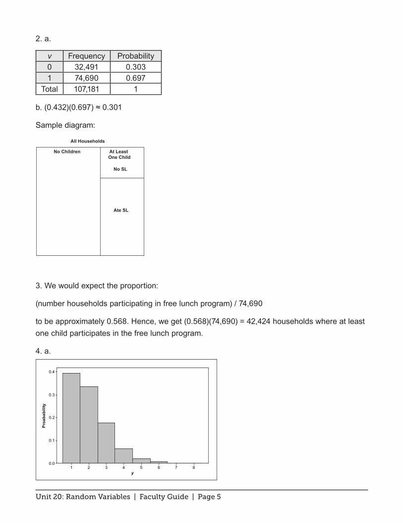
2. a.

v Frequency Probability0 32,491 0.3031 74,690 0.697

Total 107,181 1

b. (0.432)(0.697) ≈ 0.301

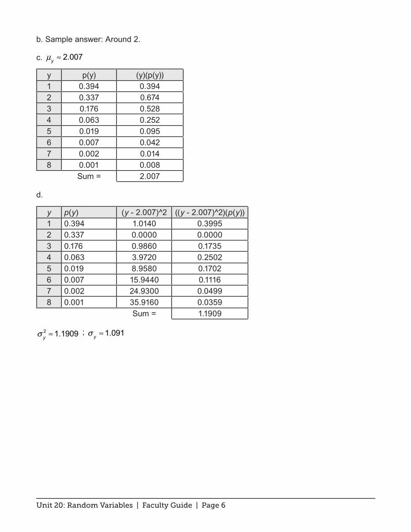
Sample diagram:

3. We would expect the proportion:

(number households participating in free lunch program) / 74,690

to be approximately 0.568. Hence, we get (0.568)(74,690) = 42,424 households where at least one child participates in the free lunch program.

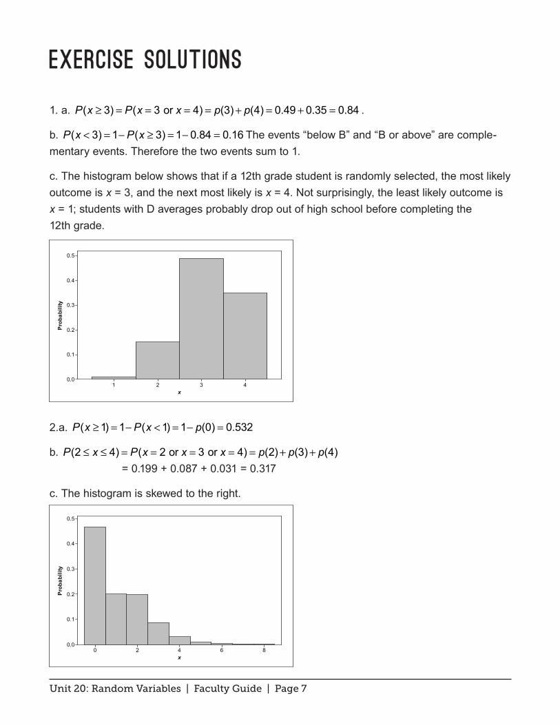
4. a.

All Households

No Children At Least One Child

No SL

Ate SL

87654321

0.4

0.3

0.2

0.1

0.0

y

Proa

babi

lity


b. Sample answer: Around 2.

c. µy ≈ 2.007

y p(y) (y)(p(y))1 0.394 0.3942 0.337 0.6743 0.176 0.5284 0.063 0.2525 0.019 0.0956 0.007 0.0427 0.002 0.0148 0.001 0.008

Sum = 2.007

d.

y p(y) (y - 2.007)^2 ((y - 2.007)^2)(p(y))1 0.394 1.0140 0.39952 0.337 0.0000 0.00003 0.176 0.9860 0.17354 0.063 3.9720 0.25025 0.019 8.9580 0.17026 0.007 15.9440 0.11167 0.002 24.9300 0.04998 0.001 35.9160 0.0359

Sum = 1.1909

σ y2 ≈1.1909 ; σ y ≈1.091


Exercise Solutions

1. a. P(x ≥ 3) = P(x = 3 or x = 4) = p(3)+ p(4) = 0.49 + 0.35 = 0.84 .

b. P(x < 3) = 1−P(x ≥ 3) = 1− 0.84 = 0.16 The events “below B” and “B or above” are comple-mentary events. Therefore the two events sum to 1.

c. The histogram below shows that if a 12th grade student is randomly selected, the most likely outcome is x = 3, and the next most likely is x = 4. Not surprisingly, the least likely outcome is x = 1; students with D averages probably drop out of high school before completing the 12th grade.

2.a. P(x ≥1) = 1−P(x <1) = 1− p(0) = 0.532

b. P(2 ≤ x ≤ 4) = P(x = 2 or x = 3 or x = 4) = p(2)+ p(3)+ p(4) = 0.199 + 0.087 + 0.031 = 0.317

c. The histogram is skewed to the right.

4321

0.5

0.4

0.3

0.2

0.1

0.0

x

Prob

abili

ty

86420

0.5

0.4

0.3

0.2

0.1

0.0

x

Prob

abili

ty


d. µ = 1.068 children under 15 per household. The calculations follow:

0 × 0.468 + 1 × 0.200 + 2 × 0.199 + 3 × 0.087 + 4 × 0.031 + 5 × 0.009 + 6 × 0.003 + 7 × 0.002 + 8 × 0.001 = 1.068 child per household.

3. a. The histogram for Distributor 1 is skewed to the right and the histogram for Distributor 2 is symmetric.

b. Using the approach outlined in the unit activity, we get µx = 1 and µy = 1 .

x or y p(x) p(y) (x)(p(x)) (y)(p(y))0 0.40 0.15 0 01 0.33 0.70 0.33 0.72 0.18 0.15 0.36 0.33 0.05 0 0.15 04 0.04 0 0.16 0

Sum = 1 1

c. Using the approach outlined in the unit activity, we get σ x2 = 1.14 and σ y

2 = 0.3 . Therefore, σ x ≈1.07 and σ y ≈ 0.55 . (Calculations follow.)

x or y p(x) p(y) ((x-1)^2)(p(x)) ((y-1)^2)(p(y))0 0.40 0.15 0.40 0.151 0.33 0.70 0 02 0.18 0.15 0.18 0.153 0.05 0 0.20 04 0.04 0 0.36 0

Sum = 1.14 0.3

43210

0.7

0.6

0.5

0.4

0.3

0.2

0.1

0.0

43210

Distributor 1

Prob

abili

ty

Distributor 2


d. For both distributors, the mean number of defects in lots of four is 1. Hence, on average, over many, many lots, there will be one defect out of four, regardless of which distributor is used. However, the standard deviations show that for Distributor 2 the number of defects is more concentrated about the mean than it is for Distributor 1. Hence, when purchasing from Distributor 1, there will be more variability in a long sequence of lots than when purchasing from Distributor 2. Given the expected number of defects out of four is the same for both dis-tributors, it makes sense to go with the distributor that has the more consistent lots.

4. a

b. P(w < 500) = 0.1846

691642593544495446397w

w500

0.1846

544


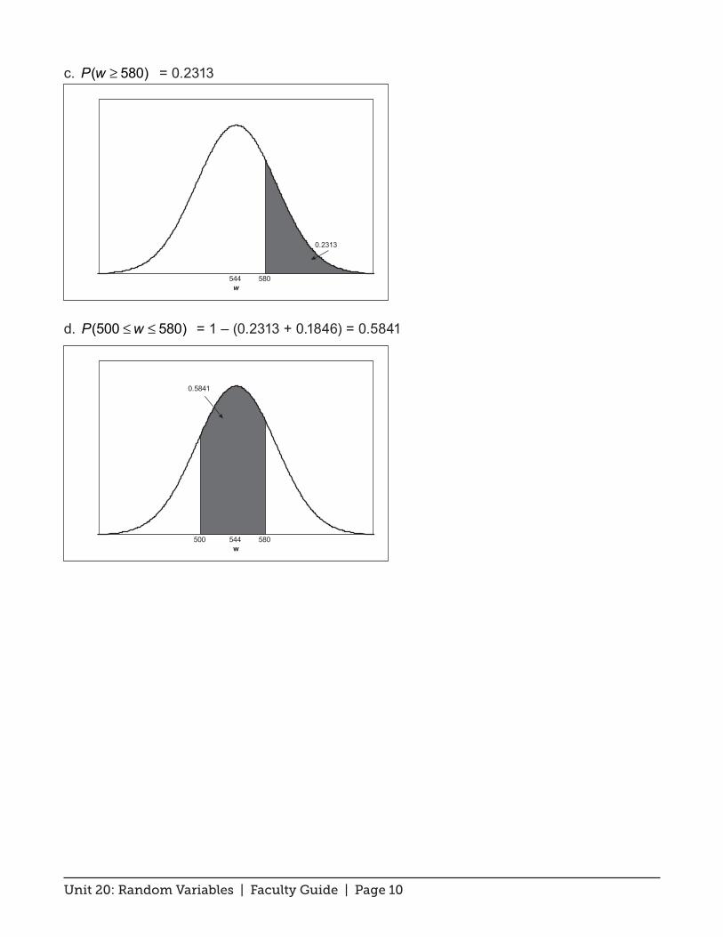
c. P(w ≥ 580) = 0.2313

d. P(500 ≤w ≤ 580) = 1 – (0.2313 + 0.1846) = 0.5841

w580

0.2313

544

w500

0.5841

580544


Review Questions Solutions

1. a. P(x < 4) = p(0)+ p(1)+ p(2)+ p(3) = 0.73 + 0.15 + 0.07 + 0.03 = 0.98.

p(4) = 1 – 0.98 = 0.02. This means that out of many, many egg cartons, roughly 2% will have four broken eggs.

b. P(x ≥ 2) = p(2)+ p(3) = p(4) = 0.07 +0.03 + 0.02 = 0.12

c.

d. µ = (0)(0.73) + (1)(0.15) + (2)(0.07) + (3)(0.03) + (4)(0.02) = 0.46. This means that in the long run, after opening many, many cartons, the average number of broken eggs is 0.46. It is also the balance point for the probability histogram.

2. a. This is an example of a discrete random variable. There will be a finite number of Cheerios in a box. The weight limit of the box adds a cap to the number of Cheerios that will fit in a box.

b. This is an example of a continuous random variable. Time to finish takes values in an interval.

c. This is discrete. Possible amounts are separated by pennies. You could put the possible amounts in a list.

Comment: In some situations, money is treated as a continuous random variable. For example, this is true for determining the amount of money in a savings account that is accruing interest. Of course, the bank always rounds down to the nearest penny when paying out money.

43210

0.8

0.7

0.6

0.5

0.4

0.3

0.2

0.1

0.0

Broken Eggs, x

Prob

abili

ty


d. Length is an example of a continuous random variable that can take values in an interval.

3. a. S = {HHH, HHT, HTH, THH, TTH, THT, HTT, TTT}

b.

x 0 1 2 3p(x) 0.125 0.375 0.375 0.125

µ = (0)(0.125)+ (1)(0.375)+ (2)(0.375)+ (3)(0.125) = 1.5

σ 2 = (0 −1.5)2(0.125)+ (1−1.5)2(0.375)+ (2−1.5)2(0.375)+ (3 −1.5)2(0.125) = 0.75

σ = 0.75 ≈ 0.866

c.

y 1 3p(y) 0.75 0.25

µ = (1)(0.75)+ (3)(0.25) = 1.5

σ 2 = (1−1.5)2(0.75)+ (3 −1.5)2(0.25) = 0.75 ; σ = 0.75 ≈ 0.866

d. In this case, the value of w is always 3.

w 3p(w) 1

µ = (3)(1) = 3

σ 2 = (3 − 3)2(1) = 0 ;σ = 0

4. a. P(w < 68) ≈ 0.2525

b. P(w ≥ 75) ≈ 0.0478

c. P(68 <w < 75) ≈ 0.6997

unit 20: random variables - annenberg learner · unit 20: random variables ... introduction to...

Documents