text mining for cross-domain knowledge discoverykt.ijs.si/theses/phd_miha_grcar.pdf · za izredno...
TRANSCRIPT

MINING TEXT-ENRICHED HETEROGENEOUS INFORMATION
NETWORKS
Miha Grčar

Doctoral Dissertation Jožef Stefan International Postgraduate School Ljubljana, Slovenia, June 2015
Evaluation Board: Asst. Prof. Igor Mozetič, Chair, Jožef Stefan Institute, Ljubljana, Slovenia
Prof. Dr. Janez Demšar, Member, Faculty of Computer and Information Science, University of Ljubljana, Ljubljana, Slovenia
Prof. Dr. Ljupčo Todorovski, Member, Faculty of Administration, University of Ljubljana, Ljubljana, Slovenia
Miha Grčar
MINING TEXT-ENRICHED HETEROGENEOUS INFORMATION NETWORKS Doctoral Dissertation
RUDARJENJE PODATKOV V TEKSTOVNO OBOGATENIH HETEROGENIH INFORMACIJSKIH OMREŽIJIH Doktorska disertacija
Supervisor: Prof. Dr. Nada Lavrač Ljubljana, Slovenia, June 2015


V
Contents
Abstract IX
Povzetek X
Abbreviations XI
1 Introduction 1
1.1 Problem description ...................................................................................................... 1
1.2 Hypothesis .................................................................................................................... 2
1.3 Objectives and contributions ........................................................................................ 3
1.4 Main publications related to the thesis ........................................................................ 5
1.5 Thesis structure ............................................................................................................ 6
2 Related work 9
2.1 Data mining ................................................................................................................. 9
2.2 Text mining ................................................................................................................ 10
2.3 Network analysis and heterogeneous network mining ................................................. 12
2.4 Data fusion for mining heterogeneous data ................................................................ 13
3 Requirements and methodology overview 15
3.1 Motivating examples ................................................................................................... 15
3.1.1 Papers and authors network example ............................................................ 15 3.1.2 Ontology querying example ........................................................................... 17
3.2 Requirements .............................................................................................................. 17
3.3 Overview of the methodology for mining text-enriched information networks ........... 19
3.4 Overview of the methodology for ontology querying .................................................. 21
3.5 Relating the two methodologies .................................................................................. 22
4 Text mining framework 23
4.1 Text mining background ............................................................................................. 23
4.1.1 Bag-of-words representation of texts ............................................................. 23 4.1.2 Basic operations in BOW spaces ................................................................... 27 4.1.3 Selected classification techniques ................................................................... 29 4.1.4 Selected clustering techniques ....................................................................... 33
4.2 Implementation of selected text mining techniques in the ClowdFlows platform ....... 35
4.3 Software availability ................................................................................................... 42
VI Contents
5 TEHmINe methodology for mining text-enriched heterogeneous information networks 43
5.1 Network mining background ....................................................................................... 43
5.1.1 Basic concepts and notations ........................................................................ 43 5.1.2 Iterative classification .................................................................................... 45 5.1.3 Diffusion kernels ............................................................................................ 46 5.1.4 Spectral clustering ......................................................................................... 47 5.1.5 PageRank and Personalized PageRank ......................................................... 48 5.1.6 SimRank ........................................................................................................ 50
5.2 Embedding networks into BOW-like spaces ............................................................... 51
5.2.1 Argumentation for choosing Personalized PageRank .................................... 52 5.2.2 Similarity measure in the PPR vector space ................................................. 53 5.2.3 Decomposing heterogeneous networks into homogeneous graphs .................. 54 5.2.4 Fusing context vectors with BOW vectors .................................................... 57
5.3 Efficient graph-based classification ............................................................................. 58
5.3.1 Multi-context nearest centroid classifier ........................................................ 58 5.3.2 PPR-based nearest centroid classifier ............................................................ 59
5.4 Complete TEHmINe workflow and its components .................................................... 60
5.5 Software availability ................................................................................................... 62
6 OntoBridge methodology for ontology querying 63
6.1 Ontologies as text-enriched heterogeneous networks .................................................. 63
6.1.1 Viewing ontologies as heterogeneous networks .............................................. 64 6.1.2 Enriching ontologies with texts ..................................................................... 65
6.2 Ontologies as homogeneous graphs ............................................................................. 66
6.2.1 Processing queries ......................................................................................... 66 6.2.2 Processing structure ...................................................................................... 67
6.3 Software availability ................................................................................................... 71
7 VideoLectures.net categorization use case 73
7.1 Problem definition ...................................................................................................... 73
7.2 Dataset ....................................................................................................................... 73
7.3 Results of text mining and diffusion kernels ............................................................... 74
7.4 TEHmINe results ........................................................................................................ 76
7.5 Time and space complexity analysis ........................................................................... 79
7.6 Visualization-guided analysis ...................................................................................... 80
8 Ontology querying use case 84
8.1 Experimental setting .................................................................................................. 84
8.1.1 Dataset and gold standard ............................................................................ 84 8.1.2 Evaluation metric .......................................................................................... 85
8.2 Evaluation results ....................................................................................................... 86
VII
8.2.1 Baseline algorithm ......................................................................................... 87 8.2.2 Graph-based algorithms ................................................................................ 89
9 Conclusions and further work 93
9.1 Review of the methodology with respect to the requirements .................................... 93
9.2 Summary of contributions .......................................................................................... 95
9.3 Future work ................................................................................................................ 96
Acknowledgements 99
References 101
Online references 109
Figures 111
Tables 113
Author’s bibliography 115
Biography 117


IX
Abstract
Text mining involves text preprocessing, modeling, knowledge discovery, visualization, and eval-uation techniques to discover, present, and evaluate knowledge from large collections of text documents (text corpora). This thesis addresses the problem of discovering knowledge from large text corpora enriched with relational links between the texts. If different relations are involved, such relational data can be described in the form of a heterogeneous information network, a generalization of the standard information network involving a single relation between the net-work nodes. If viewed from the network analysis perspective, the same problem can be interpreted as the problem of discovering knowledge from heterogeneous information networks enriched with texts. We call such networks text-enriched heterogeneous information networks or TEHINs for short.
The main hypothesis researched in the thesis is that structural/relational data, often available in real-world scenarios, can be exploited to improve the performance of algorithms employed for solving text mining tasks such as text classification and ranking. To support this hypothesis, the developed methodology should be applicable to a wide range of data analysis problems, and to large corpora of text documents accompanied with relatively large heterogeneous information networks. The main motivation for this work is due to the fact that the current general-purpose text mining tools are unable to handle texts and relational information in a common knowledge discovery setting. The goal of this thesis is thus to develop a general-purpose methodology for mining TEHINs in a typical text mining framework.
The main contribution of this thesis is the developed methodology for mining text-enriched heterogeneous information networks, named TEHmINe. It is designed as an easy-to-understand workflow, composed of well-established data and text mining components. The main functionality of the developed workflow is the projection of texts and structures into a common vector space in which knowledge discovery is performed. The methodology can be applied to a wide range of data mining problems that involve heterogeneous networks, texts, or a combination of the two data types. As an example, we show how a set of methodology building blocks can be used for very efficient centroid-based classification of vertices in heterogeneous networks and for drawing relatively large graphs and networks.
We showcase the developed methodology in two real-world use cases. In the video lecture categorization use case, we employ the TEHmINe methodology to mine a TEHIN formed out of textual data and structured information. We show that the TEHIN contains a lot of useful infor-mation and that by employing the methodology, we are able to significantly outperform the standard text mining approach. Furthermore, in the ontology querying use case, the general idea is to rank ontology entities with respect to a search query. To this end, we have adapted the proposed methodology for the task of ontology querying. We refer to the derived approach as the OntoBridge methodology. It is shown that by combining textual data and relational structure, we can significantly improve the performance of the developed ranking system over the baseline achieved with a standard text mining approach.
X Povzetek
Povzetek
Znanstveno področje rudarjenja besedil združuje postopke predobdelave besedil, izgradnje modelov, vizualizacije in evalvacije s ciljem odkrivanja, predstavitve in evalvacije znanja v velikih zbirkah (korpusih) besedil. To doktorsko delo naslavlja problem odkrivanja znanja v velikih zbirkah besedil, obogatenih z relacijskimi povezavami med besedili. Kadar so te relacije različnih tipov, lahko tak podatkovni nabor opišemo s heterogenim informacijskim omrežjem, tj. posplošitvijo standardnega modela omrežja z enim samim tipom relacije med vozlišči. Če pogledamo na ta problem z vidika analize omrežij, ga lahko interpretiramo kot problem odkrivanja znanja v heterogenih informacijskih omrežjih, obogatenih z besedili. Takim heterogenim omrežjem rečemo tekstovno obogatena heterogena informacijska omrežja.
Glavna hipoteza tega doktorskega dela je, da lahko strukturni (relacijski) podatki, ki so večkrat na voljo v realnih scenarijih rudarjenja besedil, pripomorejo k izboljšanju delovanja algoritmov za reševanje problemov, kot sta klasifikacija in rangiranje besedil. Da bi podprli to hipotezo, smo razvili metodologijo, s katero se da nasloviti različne analitske probleme in relativno velike podatkovne nabore. Glavni motiv za to delo je dejstvo, da obstoječa splošna orodja za tekstovno rudarjenje ne obravnavajo informacij o relacijah med besedili v nekem enotnem, skupnem okolju za odkrivanje znanja. Cilj tega doktorskega dela je torej razviti splošno metodologijo za rudarjenje v tekstovno obogatenih omrežjih v tipičnem okolju za tekstovno rudarjenje.
Glavni doprinos tega doktorskega dela je razvita metodologija za rudarjenje heterogenih informacijskih omrežij, obogatenih z besedili, poimenovana TEHmINe. Osnovana je kot enostavno razumljiv delotok, sestavljen iz uveljavljenih gradnikov za podatkovno in tekstovno rudarjenje. Osnovna funkcionalnost izdelanega delotoka je projekcija besedil in pripadajoče strukture v skupen vektorski prostor, v katerem lahko odkrivamo znanje. Metodologijo lahko uporabimo za reševanje različnih problemov, ki vključujejo heterogena omrežja, zbirke besedil ali kombinacijo obojega. Kot primer pokažemo, da lahko gradnike predlaganega delotoka uporabimo za izredno učinkovito klasifikacijo vozlišč omrežja z metodo najbližjih centroidov in za risanje relativno velikih grafov in omrežij.
Izdelano metodologijo preizkusimo na dveh realnih primerih. Pri primeru kategorizacije videoposnetkov predavanj uporabimo metodologijo TEHmINe za rudarjenje besedil, vključenih v heterogeno strukturno omrežje podatkov. Pokažemo, da vsebuje heterogeno omrežje veliko koristnih informacij in da dobimo z uporabo predlagane metodologije boljše rezultate kot s standardnim postopkom rudarjenja besedil.
Naslednji primer uporabe je iskanje entitet v ontologiji, kjer je osnovna ideja rangiranje entitet glede na uporabnikovo poizvedbo. V ta namen smo metodologijo TEHmINe prilagodili za potrebe iskanja ontoloških entitet. Izvedeno metodologijo smo poimenovali OntoBridge. Pokazali smo, da lahko s kombiniranjem besedil in strukturnih podatkov izboljšamo delovanje algoritma, ki je prvotno uporabljal samo informacije, vsebovane v besedilih.
XI
Abbreviations
ADC = Annotated Document Corpus API = Application Programming Interface AUC = Area Under Curve BOW = Bag Of Words BRGM = Bureau of geological and mining research, France CRISP-DM = CRoss Industry Standard Process for Data Mining DBLP = A computer science bibliography web site hosted at Trier University in Ger-
many DBSCAN = Density-Based Spatial Clustering of Applications with Noise DE = Differential Evolution DK = Diffusion Kernels DMOZ = A multilingual open-content directory of web links DS = Discovery Science (a scientific conference) EU = European Union FPR = False Positive Rate GOC = Graph Of Concepts GOT = Graph Of Triples HIN = Heterogeneous Information Network HITS = Hubs and authorities HTML = HyperText Markup Language JSON = JavaScript Object Notation k-NN = k-Nearest Neighbors LATINO = Link Analysis and Text mINing toolbox (developed as part of this thesis) LSI = Latent Semantic Indexing MKL = Multiple Kernel Learning NCC = Nearest Centroid Classifier NLP = Natural Language Processing OGC = Open Geospatial Consortium
OntoBridge = Methodology for ontology querying (developed in this thesis) PRNCC = PageRank-based Nearest Centroid Classifier (developed in this thesis) RDR = Ripple-Down Rules REST = Representational State Transfer (a software architecture style for creating
web services) ROC = Receiver Operating Characteristic (as in “ROC curve”) RWR = Random Walks with Restart SharpNLP = An open source software library for Natural Language Processing SVM = Support Vector Machine SVMlight = A software library implementing binary SVMs SVMmulticlass = A software library implementing multi-class SVMs SWING = Semantic Web Services Interoperability for Geospatial Decision Making
(EU-funded project) TAO = Transitioning Applications to Ontologies (EU-funded project) TEHIN = Text-Enriched Heterogeneous Information Network (defined in this thesis) TEHmINe = Methodology for mining text-enriched heterogeneous information networks
(developed in this thesis)

XII Abbreviations
TF-IDF = Term Frequency—Inverse Document Frequency (a term-weighting scheme) TPR = True Positive Rate URL = Uniform Resource Locator
VOB = Visual OntoBridge system for semi-automatic annotation of web services (developed as part of this thesis)
WFS = Web Feature Service WSML = Web Service Modeling Language XML = eXtensible Markup Language COBISS = Cooperative Online BIbliographic System & Services

1
1 Introduction
This thesis proposes a new methodology for mining text-enriched heterogeneous information net-works (TEHINs). The main challenge is to effectively and efficiently handle two types of data, texts and heterogeneous information networks, in a common knowledge discovery framework. In this chapter, we provide the motivation and problem statement, hypotheses, and objectives of this work. In addition, we summarize the scientific contributions, list the main publications re-sulting from this thesis, and present the structure of the thesis.
1.1 Problem description In this thesis we address the problem of discovering knowledge in large document corpora, known as text mining. Given a corpus of labeled documents in a computer readable text format, one of the most standard text mining problems is to build a classifier with the best classification accu-racy on new, unlabeled text documents. Other text mining tasks include, for example, clustering of unlabeled documents, document ranking, and document corpora visualization.
Text mining (Feldman and Sanger, 2006), which aims at extracting useful information from collections of text documents, is a well-developed field of computer science. In the last decade, the research in this field was driven by the growth of the size and the number of document collections available in companies and organizations and especially by the rapid growth of the web. Text mining is an interdisciplinary field, adopting tools and methodologies mainly from data mining, machine learning, natural language processing, and information retrieval. Text mining is typically performed in several steps, including data preprocessing, modeling, and evaluation. The data preprocessing step plays a crucial role. In this step, documents are transformed into feature vectors according to a certain representational model and then processed with the available ma-chine learning algorithms that can handle sparse vector collections with high feature dimension-ality and continuous or binary features such as k-Nearest Neighbors (k-NN), k-Means, Support Vector Machine (SVM), and Naive Bayes (Mitchell, 1997).
This thesis addresses a more complex text mining scenario where the input is not only a set of text documents, but also relational data which implicitly or explicitly provides relations be-tween these documents. Such relational data can be described in the form of a heterogeneous information network (Sun and Han, 2012), a generalization of the standard information network. A heterogeneous information network is a weighted directed graph in which each vertex is of a certain type and each edge can be of several different types. This kind of data structure allows us to describe relatively complex relationships in which different actors interact or are interrelated in different ways. Some examples of heterogeneous information networks are communication and computer networks, transportation networks, epidemic networks, social networks, e-mail networks, citation networks, and biological networks. Such networks can also be formed from data in rela-tional databases and ontologies. In heterogeneous information networks, knowledge discovery is usually performed by resorting to approaches from the fields of social network analysis, link

2 Introduction
analysis, and graph mining, or to approaches, dedicated to mining heterogeneous information networks. The latter explicitly address heterogeneity in networks which can lead to better results.
Looking at this problem from another perspective, we could argue that we address knowledge discovery scenarios in which heterogeneous information networks are enriched with texts. This basically means that in such networks, some or all objects are associated with sets of text docu-ments. Examples of such networks include the web (interlinked HTML documents), multimedia repositories (interlinked multimedia descriptions, subtitles, slide titles, etc.), social networks of professionals (interlinked CVs), citation networks (interlinked publications), and even software code (heterogeneously interlinked code comments). From this perspective, we aim at developing a methodology for mining text-enriched heterogeneous information networks (TEHINs). Moreo-ver, we do not approach the problem from the network mining perspective but rather extend a text mining framework to solve this complex problem. To this end, we consider a TEHIN as a data structure, holding both the structural and textual data.
The main motivation behind this work comes from the fact that the current general-purpose text mining toolsets are unable to handle relational information in a common data mining setting. The goal of this thesis is thus to develop a general-purpose methodology for mining TEHINs in a typical text mining framework. This would enable a skillful text miner to incorporate structural data into his or her existing experimental setups. The main challenge is to find a way to fuse textual and structural data in a seamless, effective, and efficient way. This entails at least the following requirements: (i) the user should not need to have an extensive knowledge of network mining techniques, (ii) the methodology should be applicable to a wide variety of data analysis problems, (iii) the combination of the two types of data should usually give better results than a standard text mining approach, and (iv) the developed approach needs to be applicable to rela-tively large datasets.
1.2 Hypothesis
The main hypothesis tested in the thesis is that structural data can be exploited to improve the performance of algorithms employed for solving text mining tasks, such as text classification and ranking.
The methodology developed with the goal to support this hypothesis should also conform to certain other requirements. Most notably, it should handle heterogeneous structural and textual data in a common text mining framework and it should be applicable to a wide range of data analysis problems. Moreover, it should be conceived as an easy-to-understand data analysis work-flow, employing well-established data analysis techniques, applicable to relatively large datasets.
We confirm this hypothesis in two real-world use cases. In Chapter 7, we present a use case in categorizing video lectures hosted at VideoLectures.net, one of the largest web sites hosting video-recorded scientific and educational lectures and presentations (Online reference [15]). We employ the devised methodology to combine textual data and structure from a TEHIN formed out of the available VideoLectures.net data. We show that the TEHIN contains a lot of useful infor-mation and that by employing the devised methodology, we are able to significantly outperform the standard text mining approach. Furthermore, in Chapter 8, we present an approach to on-tology querying where the general idea is to rank ontology entities with respect to a query. The baselines were set with a standard text mining approach. We show that combining textual data and structure significantly improves the performance of the developed ranking system over the baselines.
Introduction 3
1.3 Objectives and contributions The main goal of this thesis is to develop a methodology for mining text-enriched heterogeneous information networks (TEHINs). This main goal consists of a set of objectives. In the following, we summarize the main objectives and the contributions that were made within each of these objectives. Objective 1: Provide motivation, requirements, and background for mining text-enriched hetero-geneous information networks. The contributions made in the scope of this objective are the following: • We introduce the concept of a text-enriched heterogeneous information network (TEHIN).
We argue that in many real-life data mining scenarios involving document analysis, the ac-companying data can be represented in the form of heterogeneous information networks. This kind of a dataset can be represented as a TEHIN and serve as a source of data in a data analysis process. We address such a data analysis setting by proposing a methodology that takes advantage of both types of data.
• We provide an overview of the related work from the fields of text mining, link analysis, data fusion, and heterogeneous information network mining. Furthermore, we thoroughly describe the selected text mining framework. We discuss the routine for representing texts as bag-of-words (BOW) vectors and present several classification and clustering algorithms suited for working with BOW vectors. We also thoroughly discuss several approaches to embedding graphs and networks into vector spaces.
Objective 2: Devise a conceptual workflow-based view of the methodology. The contributions made in the scope of this objective are the following: • We provide a conceptual workflow-based overview of the proposed methodology for mining
TEHINs. By setting a range of requirements to narrow down the space of possible method-ologies, we provide an initial view on the methodology relatively early in the process. The proposed methodology is based on a text mining framework. It consists of two separate pipelines, one for processing texts and the other for processing the structure of a TEHIN. The texts are projected into a BOW space. The structure, on the other hand, is projected into a set of BOW-like spaces with the use of a vector-space embedding technique. The resulting vector spaces are in the end fused together, resulting in a common vector space in which knowledge discovery is performed in a standard way.
• We argue for projecting graphs into vector spaces by using the Personalized PageRank (PPR) algorithm. The structure-processing pipeline of the methodology workflow employs a vector-space embedding technique based on PPR. We provide intuitive interpretations of similarity metrics based on dot product and cosine similarity in PPR spaces. We also show a relation-ship between PPR vectors and BOW vectors by providing an analogy based on the random writer principle.
• We present (and argue for) a technique for decomposing a heterogeneous information network into a set of graphs. Since PPR originally works on weighted directed graphs, we present an approach for decomposing a heterogeneous information network into a set of (weighted di-rected) derived graphs. We provide and argue for several desirable properties of the relation represented by the edges in a derived graph. Specifically, we claim that such relation needs to model an aspect of similarity and needs to show properties of symmetry, transitivity, and reflexivity.
4 Introduction
• We present a technique for combining BOW vectors and (several sets of) PPR vectors into combined BOW-like vectors. We present a simple and pragmatic data fusion model that we use as a building block in the proposed methodology. From a general perspective, we propose to concatenate the vectors and apply a feature weighting scheme to account for the different types of data. To explain the theoretical background, we establish a relationship between vectors and linear kernels. Furthermore, we show several desirable properties of such com-bined vectors.
• We present a very efficient way of computing graph-based centroids. In our TEHIN mining framework, the nearest centroid classifier offers very good performance and is much more efficient than many other classifiers. This motivates the development of a new graph-based nearest centroid classifier that uses PPR to compute the centroids very efficiently. We call the devised algorithm the PageRank-based nearest centroid classifier (PRNCC). The algo-rithm was evaluated both in terms of its efficiency and accuracy in the VideoLectures.net use case. It outperforms the other two tested classification algorithms (i.e., 𝑘𝑘-NN and SVM) from both these two aspects.
Objective 3: Implement the developed components. We implement the developed techniques as a software library and/or a set of workflow components. The contributions made in the scope of this objective are the following: • We implement the devised components as a software library called LATINO (Link Analysis
and Text mINing toolbOx). LATINO implements a typical text preprocessing routine in which it offers a range of algorithms and language resources for tokenization, stop word removal, stemming, lemmatization, term extraction, and term weighting. In addition, the library pro-vides a collection of algorithms for supervised and unsupervised learning, most notably for classification and clustering, including the nearest centroid classifier, support vector machine, naive Bayes, and 𝑘𝑘-means clustering. LATINO is publicly available under the MIT open source license.
• We provide some of the functionality of LATINO as a set of components in a web-based data mining workflow construction and execution framework called ClowdFlows. We implement a set of wrappers that expose some of the functionality of LATINO as a set of ClowdFlows components. Instead of discussing the underlying software library, we present these compo-nents in this thesis. We present workflows and their components for text preprocessing, clas-sification, clustering, and for preprocessing TEHINs.
Objective 4: Showcase the methodology in real-life use cases. We employ the developed method-ology in two separate real-life use cases. The contributions made in the scope of this objective are the following: • We develop an automatic categorization tool for video lectures hosted at VideoLectures.net.
We employ the devised methodology to combine textual data and structure from a TEHIN formed out of the available VideoLectures.net data. We compare the methodology-based classifiers with a standard text mining routine and diffusion kernels (DK), which set relatively high accuracy standards. Our approach manages to beat these standards. It outperforms the standard text mining routine for 19% on the top-1 metric and for 10.4% on the top-10 metric. This confirms our claim that a lot of useful information is available in the structure of a TEHIN.
• We devise an approach to drawing relatively large graphs by using our vector-space embedding technique and provide means for visualization-based exploration of graphs and vector spaces.

Introduction 5
In the scope of the VideoLectures.net use case, we visualize the graphs extracted from the TEHIN by using a distance-preserving projection of PPR vectors onto a 2-dimensional plane. This technique was originally developed for visualizing collections of texts (i.e., collections of BOW vectors). We thus showed that our vector-space embedding technique can also be used for drawing relatively large graphs. Furthermore, it can also be used for visualizing collections of vectors from a fused vector space produced by our methodology.
• We devise an approach to representing ontologies as graphs. In the scope of the ontology querying use case, we design two different approaches to representing ontologies as graphs (called the graph-of-concepts and graph-of-triples, respectively). This replaces two steps in the proposed methodology: the TEHIN decomposition step and the data fusion step. The development of these new steps was required due to a very high level of heterogeneity in an ontology-based TEHIN.
• We devise and evaluate an approach to ontology querying. We develop a system for retrieving entities (i.e., concepts and domain-relation-range triples) from an ontology. The general idea is to rank ontology entities according to a user’s query. The baselines are set with a standard text mining approach. We show that combining textual data and structure—by using the developed ontology-querying methodology—improves the performance of the developed que-rying system over the baselines. The concept ranking is improved for 5.47% over the baseline area-under-curve (AUC) and the triple ranking for 3.18%.
• We implement Visual OntoBridge (VOB), a software application for supporting the user in semantic annotation tasks. On one hand, VOB provides functionality to annotate resource schemas manually. This means that the user has the ability to browse the domain ontology, select concepts relevant for the annotation at hand, and interconnect them as appropriate. On the other hand, the user can enter a set of Google-like queries to retrieve concepts and domain-relation-range triples potentially relevant for the annotation. This search functional-ity is based on the devised approach to ontology querying.
1.4 Main publications related to the thesis
The methodology for mining TEHINs outlined in Chapter 5, together with the video lecture categorization use case presented in Chapter 7, was presented at the Discovery Science conference in Espoo, Finland (Grčar and Lavrač, 2011). An extended version of this work was subsequently published in The Computer Journal (Grčar et al., 2013). Some of the research, leading to these publications, was first published as a project report in the course of the EU project TAO, Tran-sitioning Applications to Ontologies (Online reference [16]). In addition, the specific implemen-tation of the least-squares meshes algorithm, employed in the lecture categorization use case for drawing graphs, was presented at the Discovery Science conference in Canberra, Australia (Grčar et al., 2010). The video lecture categorization software prototype was also presented at ECML-PKDD in Bled, Slovenia (Grčar et al., 2009a).
The methodology for ontology querying was presented at the Pacific Rim International Con-ference on Artificial Intelligence (PRICAI) in Kuching, Malaysia (Grčar et al., 2012). The pre-liminary research, leading to this publication, was published as a project report in the course of the EU project SWING, Semantic Web Services Interoperability for Geospatial Decision Making (Andrei et al., 2008). A related paper on term matching in semantic networks was subsequently

6 Introduction
published by Springer (Grčar et al., 2009b). The ontology querying software prototype was also presented at ECML-PKDD in Bled, Slovenia (Grčar and Mladenić, 2009).
The following author’s publications are related to this thesis: • Grčar, M.; Trdin, N.; Lavrač, N. A Methodology for Mining Document-Enriched Heteroge-
neous Information Networks. The Computer Journal 56(3), 321–335, SCI IF 0.888 (2013). • Grčar, M.; Lavrač, N. A Methodology for Mining Document-Enriched Heterogeneous In-
formation Networks. In: Proceedings of the 14th International Conference on Discovery Science, Lecture Notes in Computer Science 6926, 107–121 (Springer, Berlin, Heidelberg, New York, 2011).
• Grčar, M.; Podpečan, V.; Juršič, M.; Lavrač, N. Efficient Visualization of Document Streams. In: Proceedings of the 13th International Conference on Discovery Science, Lecture Notes in Computer Science 6332, 174–188 (Springer, Berlin, Heidelberg, New York, 2010).
• Grčar, M.; Mladenić, D.; Keše, P. Semi-Automatic Categorization of Videos on VideoLec-tures.net. In: Proceedings of the European Conference on Machine Learning and Principles and Practice of Knowledge Discovery in Databases (ECML-PKDD), Lecture Notes in Com-puter Science 5782, 726–729 (Springer, Berlin, Heidelberg, New York, 2009).
• Grčar, M.; Podpečan, V.; Sluban, B.; Mozetič, I. Ontology Querying Support in Semantic Annotation Process. In: Proceedings of the 12th Pacific Rim International Conference on Artificial Intelligence (PRICAI), Lecture Notes in Computer Science 7458, 76–87 (Springer, Berlin, Heidelberg, New York, 2012a).
• Andrei, M.; Berre, A.; Costa, L.; Duchesne, P.; Fitzner, D.; Grčar, M.; Hoffmann, J.; Klien, E.; Langlois, J.; Limyr, A.; Maue, P.; Schade, S.; Steinmetz, N.; Tertre, F.; Vasiliu, L.; Zaharia, R.; N, Z. SWING: An Integrated Environment for Geospatial Semantic Web Ser-vices. In: Proceedings of the 6th European Semantic Web Conference (ESWC), Lecture Notes in Computer Science 5021, 767–771 (Springer, Berlin, Heidelberg, New York, 2008).
• Grčar, M.; Klien, E.; Novak, B. Using Term-Matching Algorithms for the Annotation of Geo-services. In: Berendt, B. et al. (eds) Knowledge Discovery Enhanced with Semantic and Social Information, Studies in Computational Intelligence 220, 127–143 (Springer, Berlin, Heidelberg, New York, 2009b).
• Grčar, M.; Mladenić, D. Visual OntoBridge: Semi-Automatic Semantic Annotation Soft-ware. In: Proceedings of the European Conference on Machine Learning and Principles and Practice of Knowledge Discovery in Databases (ECML-PKDD), Lecture Notes in Computer Science 5782, 726–729 (Springer, Berlin, Heidelberg, New York, 2009).
1.5 Thesis structure After setting grounds for this thesis by presenting the motivation, hypotheses, goals, contribu-tions, and thesis structure in Chapter 1, we provide an overview of the related work in Chapter 2. Discovering knowledge in a heterogeneous setup envisioned in this thesis requires us to address two different fields of computer science, (i) text mining and (ii) mining heterogeneous information networks. In Chapter 2, we thus briefly discuss the related work from these two fields of science. We also touch upon some other fields (such as data mining, machine learning, and data fusion) that we explore to devise the necessary parts of our methodology.
In Chapter 3, we first present two motivating examples. The first one is based on a network of scientific publications and the second one on a simple ontology used in a semantic annotation

Introduction 7
process. In addition, we set several requirements to narrow down the infinite space of all possible methodologies. Most importantly, these requirements define the scope of the methodology in terms of input data and applicability. Specifically, it is required that (i) the methodology is able to handle both texts and structure of a TEHIN, (ii) it is able to handle heterogeneity in the structure of a TEHIN, and (iii) it is generally applicable (i.e., to the extent of a typical data mining framework). The latter and also a set of other requirements suggest basing the method-ology on an existing data mining framework. The framework of our choice is a text mining framework based on the bag-of-words (BOW) representation of texts. This choice enables us to provide an initial workflow-based view on the methodology. To demonstrate the versatility of the methodology, we also present a methodology for ontology querying (related to the second moti-vating example), which we construct from the building blocks of the proposed methodology.
The two proposed methodologies—the general-purpose TEHIN mining methodology named TEHmINe and the ontology querying methodology named OntoBridge—are based on a text mining framework. In Chapter 4, we present this framework—specifically the text preprocessing routine and several suitable machine learning algorithms—and discuss the related theoretical background. The described text mining techniques are implemented as part of this thesis as a software library called LATINO (Link Analysis and Text Mining Toolbox). A large part of LATINO is also made available in the ClowdFlows platform, i.e., a web-based platform for com-posing and executing data mining workflows by means of visual programming. We present the implemented ClowdFlows components in the second part of this chapter.
In Chapter 5, we develop the structure preprocessing part of TEHmINe. This provides a complete specification of the methodology and the grounds for its implementation. To provide the basis for devising the structure-preprocessing part of the methodology, we first present several approaches from network analysis for embedding networks into vector spaces. We then argue for the use of Personalized PageRank (PPR) in the structure preprocessing phase by providing intu-itive interpretations of similarity metrics in PPR spaces. Moreover, we show a relationship be-tween PPR vectors and BOW vectors by providing an analogy based on the random writer principle. Since PPR originally works on directed weighted graphs, we show how to decompose a heterogeneous information network into a set of directed weighted graphs. As the last missing piece, we discuss the process of fusing different modalities of a heterogeneous information network and the accompanying texts into a common vector space in which knowledge discovery can be performed. In addition, we devise an algorithm for an efficient structure-based centroid compu-tation with PPR. The use of this centroid-computation technique in the classical nearest centroid classifier substantially speeds up its training phase. In the last part, we give a specification for implementing the structure preprocessing components in ClowdFlows.
In Chapter 6, we present the ontology querying methodology named OntoBridge. This meth-odology is derived from the general-purpose TEHIN mining methodology. However, it has certain specifics that we thoroughly discuss in this chapter. First, we present two different approaches to transforming ontologies into TEHINs (called the graph-of-concepts and graph-of-triples, respec-tively). These texts were formed from search-result snippets obtained by querying a web search engine. We present a different data fusion approach required due to a high level of heterogeneity in an ontology-based TEHIN: we use textual data to assign weights to the edges thus forming a weighted directed graph. Such a graph can then be used for further analysis.
In Chapter 7, we present the video lecture categorization use case. The aim of this use case is to develop an automatic categorization tool for video lectures hosted at VideoLectures.net, one of the world’s largest scientific and educational video web sites. A snapshot of the database

8 Introduction
provided to us contained 3,520 lectures, 1,156 of which were manually categorized. The taxonomy into which the lectures were categorized contained 129 categories. We employed the developed methodology to combine textual data and structure from a TEHIN formed out of the available VideoLectures.net data. We decomposed the TEHIN into three graphs that we called the viewed-together, same-author, and same-event graph. We compared our methodology with the standard text mining routine and diffusion kernels (DK). Both these two competitors set relatively high standards. The proposed methodology managed to beat these baselines. It outperformed the standard text mining routine for 19% on the top-1 metric and for 10.4% on the top-10 metric (in absolute terms). This confirms our claim that a lot of useful information is available in the structure of a TEHIN. In this chapter, we also present a visualization-guided analysis which reveals that derived graphs with many disconnected components are unable to perform well when not used in a combination with other types of data. For the purpose of this analysis, we use a distance-preserving projection of PPR vectors onto a 2-dimensional plane. This technique was originally developed for visualizing collections of texts (i.e., collections of BOW vectors). We thus show that our methodology can also be used for drawing relatively large graphs.
In Chapter 8, we present the ontology querying use case. The aim is to develop a system for retrieving entities (i.e., concepts and domain-relation-range triples) from an ontology. The general idea is to rank ontology entities with respect to a user’s query. The baselines are set with a standard text mining approach. We show that combining textual data and structure improves the performance of the developed ranking system over the baselines. The concept ranking is improved for 5.47% over the baseline area-under-curve (AUC) and the triple ranking for 3.18% (in absolute terms).
In Chapter 9, we first review the TEHmINe methodology with respect to the requirements defined in Chapter 3. Finally, we conclude the thesis by presenting several ideas for further work.
9
2 Related Work
Text-enriched heterogeneous information networks (TEHINs) are data structures that describe instances with two different types of data: (i) texts and (ii) heterogeneous information networks. Discovering knowledge in such a heterogeneous setup requires to employ two different fields of computer science, (i) text mining and (ii) mining heterogeneous information networks. In the following, we briefly discuss related work from these two fields of science. We also touch upon some other fields (such as data mining, machine learning, and data fusion) that we explore to devise all the necessary parts of our methodology.
2.1 Data mining Data mining originally refers to discovering knowledge from large databases (Witten et al., 2011). It employs methods mainly from the fields of database systems, artificial intelligence, machine learning, and statistics with the goal of extracting information, knowledge, and patterns from large amounts of data.
While data mining borrows its methods from other fields of science, it is itself more applica-tion-oriented and also defines a high-level process for knowledge discovery. There have been sev-eral attempts to standardize this process. The most widely known data mining process model and an industry standard for applying data mining techniques is CRISP-DM, Cross-Industry Standard for Data Mining (Shearer, 2000). It is an iterative process and consists of the following six major stages (see Figure 2.1):
1. Business understanding. This stage focuses on (i) understanding the problem and the re-quirements from a business perspective, (ii) formulating the problem as a machine learning task, and also (iii) devising a plan to solve the task.
2. Data understanding. In this stage, (i) data acquisition is performed and (ii) the data is explored in order for the analyst to get more familiar with the data format, content, and properties.
3. Data preparation. In the data preparation stage, the raw data is prepared for further pro-cessing. This involves activities such as data selection, cleaning, and transformation.
4. Modeling. In this stage, (i) various modeling techniques are applied and (ii) the resulting models are evaluated from a data analysis perspective. Note that it is often necessary to backtrack in order to prepare a more suitable dataset.
5. Validation. This stage focuses on validating the solution with respect to the business re-quirements. If the solution fails to reach the business objectives, it is necessary to repeat the entire cycle in order to improve the solution or rethink the objectives.
6. Deployment. The deployment stage focuses on delivering the results (discovered knowledge) to the end user (customer). This can be as simple as generating a report or as complex as

10 Related Work
implementing a repeatable data mining process and integrating it into the customer’s in-formation system.
Since this process is rather general, it can easily be adapted for analyzing datasets other than structured tabular data (database tables), such as texts (text mining) or graphs (graph mining). The TEHIN-mining methodology proposed in this thesis can also be aligned with this process. We mainly develop components that participate in the data preparation and modeling phase of this entire process.
2.2 Text mining Text mining (Feldman and Sanger, 2006) incorporates text preprocessing, modeling (knowledge discovery), visualization, and evaluation techniques to discover, present, and evaluate knowledge from large collections of text documents (also called text corpora). It adopts methodologies and tools most notably from data mining, machine learning, information retrieval, and natural lan-guage processing.
In contrast to a typical data mining problem, where data is expected to be in a structured tabular form, raw text documents are in general unstructured and first need to be transformed into a suitable representation. Two predominant approaches are used in practice.
In the first approach, documents are converted into high-dimensional vectors in which dimen-sions are usually terms (i.e., words and phrases) extracted from the corpus. The vectors are computed by employing several basic NLP techniques and a feature-weighting scheme (Salton, 1989). Since the order of terms is discarded in this process, such vectors are also referred to as
Figure 2.1: Cross-Industry Standard for Data Mining (CRISP-DM).
Taskdefinition
Data understanding
Data preparation
Modeling
Evaluation
DeploymentData
Related Work 11
bag-of-words vectors or simply bags-of-words (BOW). This approach originates from information retrieval, a scientific field concerned with the retrieval of information objects (such as documents) relevant to the user’s information needs. Another approach found in the literature is to convert texts into graphs of recognized entities (e.g., Feldman and Sanger (2006), Chapter XI) or ex-tracted triples (e.g., Leskovec et al. (2004)) by employing relatively complex NLP techniques such as part-of-speech tagging, chunking, and parsing. Such representation of text is then further analyzed with link analysis techniques (Getoor and Diehl, 2005; Nooy et al., 2005). In this thesis, we limit ourselves to the case where documents are represented as bag-of-words vectors in which features are words and phrases. We provide more details on this kind of BOW model and the corresponding text preprocessing routine in Section 4.1.1.
In the modeling phase of a text mining process, many different techniques to discover, extract, and organize knowledge from the preprocessed text documents can be employed. We limit our-selves to the setting where modeling is performed by the use of machine learning techniques. Machine learning is concerned with the development of algorithms that allow computer programs to learn from past experience (Mitchell, 1997). In more technical terms, machine learning refers to a collection of algorithms that take as input empirical data (e.g., from databases or sensors) and try to discover some characteristics (rules, constraints, patterns, features) of the process that generated the data. Although there exist many generally recognized categories of machine learn-ing algorithms, we only discuss supervised and unsupervised learning methods in this thesis. Within these two categories, we additionally limit ourselves to the classification and clustering algorithms, which leaves out most notably the regression methods.
Classification and regression are both instances of supervised learning where a training set of manually or otherwise correctly labeled observations is available. Classification refers to assigning an instance to one or more predefined discrete classes (in this case, the labels correspond to these classes). In contrast, regression refers to assigning a numeric value to an instance (in this case, the labels are numeric values). In both cases, a training algorithm first builds a model which contains knowledge derived from the training set. This model is then applied in the prediction phase to label new instances.
Clustering, on the other hand, is a form of unsupervised learning and is employed when train-ing labels are not available. The task of a clustering algorithm is to arrange instances into groups (i.e., clusters) so that the instances in the same group are more similar to each other than to those in the other groups. Sections 4.1.3 and 4.1.4 provide more details on the selected machine learning principles and techniques and are focusing on the algorithms that are suitable for pro-cessing bag-of-words vectors constructed in the text preprocessing phase.
Text mining techniques can be employed for solving many different tasks such as text catego-rization (also known as “text classification”), topic ontology construction (Fortuna et al., 2005), text corpora visualization (Fortuna et al., 2006; Vieira et al., 2006), and user profiling (Grčar et al., 2005; Kim and Chan, 2008). For the use cases presented in this thesis (Chapters 7 and 8), the most important tasks are text categorization and text corpus visualization.
Text categorization is a widely researched area due to its value in real-life applications such as indexing of scientific articles, patent categorization, spam filtering, and web page categoriza-tion (Sebastiani, 2002). In (Mladenić, 1998), the authors present a method for categorizing web pages into the Yahoo! taxonomy. They employ a set of Naive Bayes classifiers, one for each category in the taxonomy. For each category, the corresponding classifier gives the probability that the document belongs to this category. A similar approach is presented in (Grobelnik and
12 Related Work
Mladenić, 2005), where web pages are being categorized into the DMOZ taxonomy (Online ref-erence [11]). Each category is modeled with the corresponding centroid BOW vector and a doc-ument is categorized simply by computing the cosine similarity between the document’s BOW vector and each of the computed centroids. Nearest centroid text classification was explored also by other researchers (e.g., Han and Karypis, 2000).
Text corpora visualization techniques can be used for gaining insight into data and thus guid-ing knowledge discovery processes. Document space visualization techniques are used to provide overviews and insights into relatively large document collections. A document space is essentially a high-dimensional BOW vector space. To visualize a document space, feature vectors need to be projected onto a two-dimensional canvas so that the neighborhoods of points in the planar pro-jection reflect the neighborhoods of vectors in the original high-dimensional space. In this thesis, we employ a document space visualization technique based on least-square meshes (Sorkine and Cohen-Or, 2004; Vieira et al., 2006)—more specifically, the implementation presented in (Grčar et al., 2010)—to visualize relatively large networks (see Section 7.6).
2.3 Network analysis and heterogeneous network mining
Network analysis refers to studying relations or interactions between instances (entities). The modern network analysis approaches originate mainly from employing mathematical theories about graphs and networks in social sciences. To study human societies, exploring relationships between participants, in addition to studying their properties, became increasingly important in the early eighties (Burt and Minor, 1983). Since then, network analysis became its own field of science, covering many different types of networked data, such as bibliographic networks, online social networks, biological networks, computer networks, and transportation networks. In the area of network analysis, a different family of data analysis algorithms was devised to perform typical machine learning tasks such as ranking, classification, and clustering.
A relatively common property of network analysis algorithms is the ability to assess similarities between vertices in terms of how strongly they are interconnected. Assessing these similarities is often used to rank vertices according to how relevant they are either in general or to another vertex (or a group of vertices). Such ranking and similarity assessment methods are used in information retrieval systems where the general idea is to propagate relevance from query nodes into the rest of the network, assigning higher ranks to more relevant objects. The most well-known relevance assessment algorithm is PageRank (Page et al., 1999) which is a measure of relative importance of a vertex in a directed weighted graph. A variation of the original algorithm, called “personalized PageRank” (PPR), can be used to measure importance of a vertex with respect to another vertex or a group of vertices (Page et al., 1999). Other relevance and similarity assessment algorithms include spreading activation (Crestani, 1997), hubs and authorities (HITS) (Kleinberg, 1999), SimRank (Jeh and Widom, 2002), and diffusion kernels (DK) (Kondor and Lafferty, 2002). We discuss some of these algorithms in more details in Section 5.1.
In recent years, the concept of heterogeneous information networks (Sun and Han, 2012), a generalization of standard information networks, is gaining attention. While a (homogeneous) network is a weighted directed graph with one single type of vertices and one single type of edges, a heterogeneous information network is a weighted directed graph in which each vertex and each edge can be of a specific type. Most approaches, devised for homogeneous information networks, can also be applied to heterogeneous information networks by simply ignoring the nature of links
Related Work 13
and/or vertices. Discarding this information, however, can lead to poorer results as noted in (Davis et al., 2011).
As is the case with standard networks, ranking and similarity assessment are important tools when mining heterogeneous information networks. In the area of information retrieval, different techniques to rank objects in a heterogeneous setting were developed. ObjectRank (Balmin et al., 2004) employs global PageRank (importance) and PPR (relevance) to enhance the keyword search in databases. Specifically, the authors convert a relational database of scientific papers into a graph by constructing two graphs: the data graph (interrelated instances) and the schema graph (concepts and relations). Similarly, EntityAuthority (Stoyanovich et al. (2007)) is a ranking method which defines a graph-based data model that combines web pages, extracted (named) entities, and ontological structure in order to improve the quality of keyword-based retrieval of either pages or entities. The authors evaluate three conceptually different methods for determin-ing relevant pages and/or entities in such graphs. One of the methods is based on mutual rein-forcement between pages and entities, while the other two approaches are based on PageRank and HITS (Kleinberg, 1999), respectively.
In (Sun and Han, 2012), the authors propose a ranking technique (called “authority ranking”) for bipartite bibliographical networks in which authors are linked to their papers. The proposed ranking approach is a generalization of PageRank to bipartite networks, assigning ranks to au-thors and papers separately. Furthermore, the authors propose two algorithms, namely RankClus (Sun et al., 2009a) and NetClus (Sun et al., 2009b), which perform ranking-based clustering. The general idea behind ranking-based clustering is that highly-ranked objects within a cluster more likely belong to that cluster. These two algorithms thus iteratively perform clustering and ranking, adjusting the clusters according to the ranking results in each iteration. While RankClus can only be employed on bipartite networks, NetClus is designed to work on a more general type of networks.
To address classification problems in heterogeneous information networks, a generalized label propagation methodology of Zhou et al. (2003) can be used (Hwang and Kuang, 2010; Sun and Han, 2012). Another approach called GNetMine (Ji et al., 2010) is based on the graph regulari-zation technique originally proposed by Zhou and Schölkopf (2004) and can be used to take network heterogeneity into account. Taking the general idea of GNetMine even further, Ji et al. (2011) propose a ranking-based classification algorithm called RankClass. The general idea of ranking-based classification is that vertices connected to highly-ranked vertices within a class likely belong to this same class. RankClass employs an iterative two-step process in which (i) labels are assigned to unlabeled vertices and (ii) within-class rankings are recomputed.
The approach that we propose in this thesis differs from the aforementioned approaches mainly because it decouples the “authority propagation” technique from the notion of heterogeneity which comes into play later on, in the data fusion stage of the proposed process.
2.4 Data fusion for mining heterogeneous data This section outlines some of the related approaches to fusing heterogeneous data.
Data fusion refers to combining different types of data (media) in order to perform a data analysis task. It is widely studied in the field of multimedia analysis where data is obtained from different modalities such as video, audio, text and motion.

14 Related Work
An extensive survey is presented by Atrey et al. (2010). According to the authors of the survey, data fusion can either be performed on the feature level (early fusion) or on the decision level (late fusion). Feature-level fusion refers to combining features or feature vectors in the data transformation process. Propositionalization (Kramer et al., 2001), an approach well known from inductive logic programming (Lavrač and Džeroski, 1994; Muggleton, 1992) and relational data mining (Džeroski and Lavrač, 2001), belongs to this category of data fusion techniques. It refers to the process of converting a relational knowledge representation into a propositional feature vector representation. An extensive survey of propositionalization approaches can be found in (Kramer et al., 2001). Feature-level fusion is advantageous in that the employed training algo-rithm can study correlations between features, which is not possible with the decision-level ap-proaches.
On the other hand, decision-level fusion refers to solving the task for each modality separately and then combining the results through a fusion model (e.g., Caruana et al., 2006; Getoor and Diehl, 2005). One of the simplest late fusion approaches is majority voting which is often used in ensembles of machine learning models. If the data mining approach is based on the probabilistic framework (e.g., Naive Bayes, logistic regression, maximum entropy model), it is possible to perform fusion by using Bayesian inference (e.g., Lu and Getoor, 2003). The decision-level ap-proaches have the advantages of (i) being more scalable (several smaller models are built instead of one large model), (ii) allowing the use of different models in the inference phase and (iii) providing a uniform representation of data (i.e. a set of decisions) that is further processed with a fusion model.
We additionally point out that data fusion can also be performed at the kernel level, which corresponds to combining kernels over different modalities. The most obvious advantage of this type of fusion, similarly to the decision-level approaches, is that the fusion model deals with a uniform data representation (i.e. a set of kernels). One of the disadvantages is that only the kernel-based data analysis algorithms can be employed after the fusion process. Lanckriet et al. (2004) propose a general-purpose methodology for kernel-based data fusion. They represent each type of data with a kernel and then compute a weighted linear combination of kernels (which is again a kernel). The linear-combination weights are computed through an optimization process called Multiple Kernel Learning (MKL) (Rakotomamonjy et al., 2008; Vishwanathan et al., 2010), integrated into the SVM’s margin maximization process. The authors define a quadratically con-strained quadratic program in order to compute the support vectors and linear-combination weights that maximize the margin. In the paper, the authors employ their methodology for pre-dicting protein functions in yeast. They fuse together six different kernels (four of them are diffusion kernels based on graph structures). They show that their data fusion approach outper-forms the SVM trained on any single type of data, as well as the previously advertised method based on Markov random fields. In the approach that we employ in our use case (see Section 7), we do not employ MKL but rather a stochastic optimizer called differential evolution (DE) (Storn and Price, 1997), which enables us to directly optimize the target evaluation metric.
15
3 Requirements and Methodology Overview
In this chapter, we give an overview of the proposed TEHmINe methodology. We also present a methodology for ontology querying which we derive from TEHmINe and thus demonstrate its versatility. We provide motivating examples, requirements, and discuss the two methodologies in terms of conceptual data mining workflows.
3.1 Motivating examples
A data mining task often involves data in the form of heterogeneous information networks in which (some) objects are associated with texts (e.g., the web, social networks, e-mail networks, text-enriched ontologies, etc.). In the following, we present two examples that motivate us to create and mine text-enriched heterogeneous information networks.
3.1.1 Papers and authors network example
One of the most typical scenarios involving text-enriched heterogeneous information networks (TEHINs) is analyzing a social network of researchers that publish papers, such as the DBLP database (Ley, 2002). A very similar situation occurs in almost every social network where the participants generate some textual content. For this reason, a small made-up DBLP-like network will serve us as a toy example when discussing different aspects of the proposed methodology in this chapter (and also later in Chapter 5).
Figure 3.1 shows this toy TEHIN. Let us first imagine a dataset from which we have built this network. Suppose that the dataset contains a collection of conference papers, and that for each paper, the following data and meta-data are available:
• Title, body text (main content) • List of authors • Conference proceedings in which the paper was published (e.g., Proceedings of Discovery
Science 2010) • Year of publication (e.g., 2010) • Citation references
The first thing to note here is that the process of building a network from this dataset is not a completely trivial task. The process is as follows. First, we identify the types of objects that will be represented as vertices in the resulting network. These are papers, authors, and proceed-ings. Note that it is sometimes not trivial to tell which data items represent the same network object. For example, the author “Nada Lavrač” can appear in the meta-data as “Nada Lavrač”, “N. Lavrac”, “N Lavrač”, or in some other form. It is crucial to devise a mapping mechanism that resolves this problem and maps different names (references) of the same object to the same unique object identifier.

16 Requirements and Methodology Overview
Secondly, we identify the types of links that we will establish between these objects. There are many different ways to do this and there is no general rule. For example, an author can be linked to each of his papers with “author of” links or, the other way around, a paper can be linked to each of its authors with “written by” links. The links can even go both ways. In fact, every link forming a relation normally has its inverse counterpart. Moreover, an author can be linked to a proceedings with a “published a paper in” link or, less directly, an author can first be related to a paper and then this paper links to the proceedings in which it was published. In the particular case presented in Figure 3.1, we link an author to each of his papers with an “author of” link. Furthermore, we link a paper to the corresponding proceedings with a “published in” link. Finally, we link two papers with a “cites” link if the first paper cites the second one. We also incorporate additional knowledge (background, common knowledge) about how proceedings can be grouped into series of annual publications. For example, Proceedings of Discovery Science 2010 (DS 2010) and Proceedings of Discovery Science 2011 (DS 2011) are both proceedings of the DS conference series. Even though this seems like adding some obvious information, it can make a big difference when inferring a structure from these data. Since DS 2010 and DS 2011 are in fact two different events, a relationship between a paper presented at DS 2010 and a paper presented at DS 2011 cannot be drawn without this additional background knowledge.
Thirdly, we explore the available textual data and attach texts to certain objects in the net-work. In our case, we first form a textual representation of a paper by joining (concatenating) its title and its body text. This gives us a collection of texts, each corresponding to a particular paper. We attach each text to the vertex representing the corresponding paper, which finally gives us a TEHIN.
The resulting network represents the source of data in a data mining process. In this process, the main “driving force” is the task at hand. The video lecture categorization use case that we present in Chapter 7 also deals with a very similar heterogeneous information network: a social network of authors who present their work at conferences, workshops, and similar scientific events. In this particular use case, the task is to develop a method that can be used to support the categorization of video lectures hosted by VideoLectures.net, one of the world’s largest scientific and educational video web sites.
Figure 3.1: Toy heterogeneous information network of conference papers.
Paper2
Paper4
DS 2011
DS
DS 2010
authorOf
authorOf
publishedIn
publishedIn
is-a is-a
Paper3
authorOf
publishedIn
cites
authorOf
authorOf
Paper1
authorOf
PRICAI2008
publishedIn
cites

Requirements and Methodology Overview 17
3.1.2 Ontology querying example
Semantic annotations are formal, machine-readable descriptions that enable efficient search and browse through resources, as well as efficient composition and execution of web services. In this work, the semantic annotation is defined as a set of interlinked ontology elements related to the resource in question. For example, let us assume that our resource is a database table. We want to annotate its fields in order to provide compatibility with databases from other systems. Further on, let us assume that this table has a field called “employee_name” that contains employee names (as given in Figure 3.2, left side). On the other hand, we have a domain ontology containing knowledge and vocabulary about companies (an excerpt is given in Figure 3.2, right side). In order to state that the table field in fact contains employee names, we first create a variable of type Name (Name is a domain-ontology concept) and associate it with the field. We then create a variable of type Person and link it to the variable of type Name via the hasName relation. Finally, we create a variable of type Company and link it to the variable of type Person via the hasEmployee relation. Such annotation (shown in the middle in Figure 3.2) indeed holds the desired semantics: the annotated field contains names of people which some company employs (i.e., names of employees).
Note that it is possible to replace any of the variables with an actual instance representing a real-world entity. For example, the variable ?c could be replaced with an instance representing an actual company such as, for example, Microsoft ∈ Company. The annotation would then refer to “names of people employed at Microsoft”.
The annotation of a resource is a process in which the user (i.e., the domain expert) creates and interlinks domain-ontology instances and variables (concepts) in order to create a semantic description for the resource in question. Formulating annotations in one of the formal languages, such as WSML (Online reference [1]), is not a trivial task and requires specific expertise.
For this reason, we propose a methodology for querying ontologies. We derive it from the TEHmINe methodology and adapt it to certain specifics of the ontology querying task. We im-plement this methodology as part of Visual OntoBridge (VOB) (Grčar and Mladenić, 2009; Grčar et al., 2012), a system that provides a graphical user interface and a set of machine learning algorithms that support the user in the annotation tasks. VOB provides the functionality for querying the domain ontology with the purpose of finding the appropriate concepts and triples. A triple in this context represents two interlinked instance variables (e.g., ?Com-pany hasEmployee ?Person) and serves as a more complex building block for defining semantic annotations.
In Chapter 6, we present the ontology querying workflow and discuss how a grounded ontology can be transformed into a TEHIN. The term “grounded” in this context means that every ontol-ogy entity of interest is enriched with a set of documents describing, talking about, or otherwise being related to this entity. Such a TEHIN can then be used in a typical feature-ranking setting in which features (ontology entities) are ranked according to a search query.
3.2 Requirements In this section, we define and discuss requirements for a general-purpose methodology for mining TEHINs. With these requirements, we narrow down the space of possibilities both for the entire methodology and for its main ingredients. The complete list of requirements is as follows:

18 Requirements and Methodology Overview
1. Bimodality. The methodology (and the corresponding toolkit) needs to enable us to exploit both textual and structural aspect of a network in order to improve the performance of the developed solution over using just one or the other.
2. Heterogeneity. The methodology needs to provide facilities to handle the fact that different types of objects and different types of links are used to form the network that represents the source of data. We should be able to improve the performance of a devised solution by carefully choosing (or weighting) which types of information (links, objects) to take into account (or emphasize) and which to ignore (or suppress).
3. Applicability. The methodology needs to be applicable to a wide range of data mining problems involving text corpora, (heterogeneous) information networks, or TEHINs.
4. Uniformity. The purpose of the methodology is to join the two worlds, text mining and network analysis, in a seamless way. The same modeling (analysis) tools should be able to handle both textual and structural data from a network. Furthermore, the same toolkit needs to be applicable in the scenarios when there is only text or only structure available.
5. Maturity. The methodology should employ well-established and well-developed building blocks from the fields of text mining and network analysis. It should employ approaches that researchers are familiar with and that are known to perform well for their specific purposes.
6. Modularity. The methodology needs to be formed of a set of components arranged into a data mining workflow. This requirement accommodates the implementation of the meth-odology in a workflow-based data mining environment.
7. Efficiency. The devised methodology needs to support efficient implementation. The im-plemented toolkit needs to process small networks of up to several 10,000 vertices (and text corpora of that same size) on an ordinary (inexpensive) desktop computer in a reasonable time.
Figure 3.2: Annotation as a ‘bridge’ between a resource and the domain ontology.
employee_name...
employee
Company
Person Name
hasNamehasEmployee
hasName
?c ∈ Company
?p ∈ Person
?n ∈ Name
hasEmployee
hasName
Requirements and Methodology Overview 19
Following these requirements, we have developed the general-purpose TEHmINe methodology. Furthermore, we have reused its components in an ontology querying workflow, addressing the specifics of the ontology querying problem.
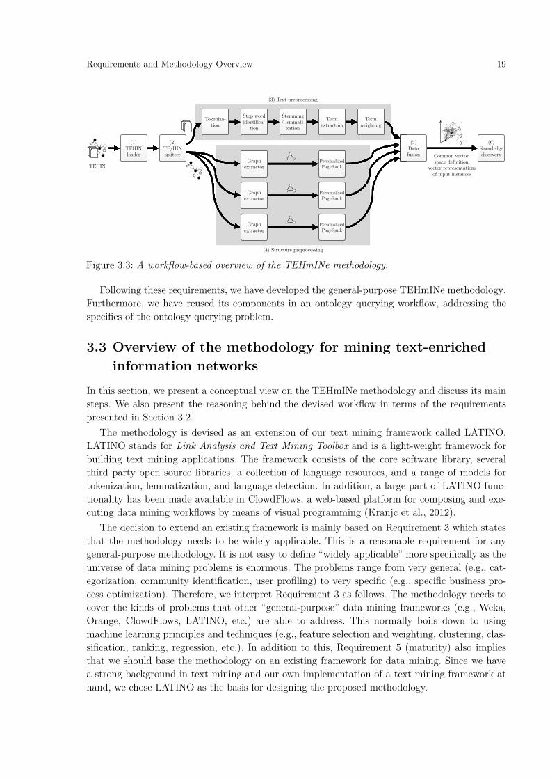
3.3 Overview of the methodology for mining text-enriched information networks
In this section, we present a conceptual view on the TEHmINe methodology and discuss its main steps. We also present the reasoning behind the devised workflow in terms of the requirements presented in Section 3.2.
The methodology is devised as an extension of our text mining framework called LATINO. LATINO stands for Link Analysis and Text Mining Toolbox and is a light-weight framework for building text mining applications. The framework consists of the core software library, several third party open source libraries, a collection of language resources, and a range of models for tokenization, lemmatization, and language detection. In addition, a large part of LATINO func-tionality has been made available in ClowdFlows, a web-based platform for composing and exe-cuting data mining workflows by means of visual programming (Kranjc et al., 2012).
The decision to extend an existing framework is mainly based on Requirement 3 which states that the methodology needs to be widely applicable. This is a reasonable requirement for any general-purpose methodology. It is not easy to define “widely applicable” more specifically as the universe of data mining problems is enormous. The problems range from very general (e.g., cat-egorization, community identification, user profiling) to very specific (e.g., specific business pro-cess optimization). Therefore, we interpret Requirement 3 as follows. The methodology needs to cover the kinds of problems that other “general-purpose” data mining frameworks (e.g., Weka, Orange, ClowdFlows, LATINO, etc.) are able to address. This normally boils down to using machine learning principles and techniques (e.g., feature selection and weighting, clustering, clas-sification, ranking, regression, etc.). In addition to this, Requirement 5 (maturity) also implies that we should base the methodology on an existing framework for data mining. Since we have a strong background in text mining and our own implementation of a text mining framework at hand, we chose LATINO as the basis for designing the proposed methodology.
Figure 3.3: A workflow-based overview of the TEHmINe methodology.
(4) Structure preprocessing
(3) Text preprocessing
Graph extractor
Personalized PageRank
Graph extractor
Graph extractor
Personalized PageRank
Personalized PageRank
Stop word identifica-
tion
Stemming / lemmati-
zation
Term extraction
Term weighting
Tokeniza-tion
(2)TE/HIN splitter
(5)Datafusion
(6)Knowledge discoveryCommon vector
space definition,vector representations
of input instances
(1)TEHIN loader
TEHIN
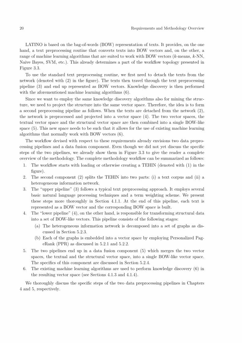
20 Requirements and Methodology Overview
LATINO is based on the bag-of-words (BOW) representation of texts. It provides, on the one hand, a text preprocessing routine that converts texts into BOW vectors and, on the other, a range of machine learning algorithms that are suited to work with BOW vectors (𝑘𝑘-means, 𝑘𝑘-NN, Naive Bayes, SVM, etc.). This already determines a part of the workflow topology presented in Figure 3.3.
To use the standard text preprocessing routine, we first need to detach the texts from the network (denoted with (2) in the figure). The texts then travel through the text preprocessing pipeline (3) and end up represented as BOW vectors. Knowledge discovery is then performed with the aforementioned machine learning algorithms (6).
Since we want to employ the same knowledge discovery algorithms also for mining the struc-ture, we need to project the structure into the same vector space. Therefore, the idea is to form a second preprocessing pipeline as follows. When the texts are detached from the network (2), the network is preprocessed and projected into a vector space (4). The two vector spaces, the textual vector space and the structural vector space are then combined into a single BOW-like space (5). This new space needs to be such that it allows for the use of existing machine learning algorithms that normally work with BOW vectors (6).
The workflow devised with respect to these requirements already envisions two data prepro-cessing pipelines and a data fusion component. Even though we did not yet discuss the specific steps of the two pipelines, we already show them in Figure 3.3 to give the reader a complete overview of the methodology. The complete methodology workflow can be summarized as follows:
1. The workflow starts with loading or otherwise creating a TEHIN (denoted with (1) in the figure).
2. The second component (2) splits the TEHIN into two parts: (i) a text corpus and (ii) a heterogeneous information network.
3. The “upper pipeline” (3) follows a typical text preprocessing approach. It employs several basic natural language processing techniques and a term weighting scheme. We present these steps more thoroughly in Section 4.1.1. At the end of this pipeline, each text is represented as a BOW vector and the corresponding BOW space is built.
4. The “lower pipeline” (4), on the other hand, is responsible for transforming structural data into a set of BOW-like vectors. This pipeline consists of the following stages:
(a) The heterogeneous information network is decomposed into a set of graphs as dis-cussed in Section 5.2.3.
(b) Each of the graphs is embedded into a vector space by employing Personalized Pag-eRank (PPR) as discussed in 5.2.1 and 5.2.2.
5. The two pipelines end up in a data fusion component (5) which merges the two vector spaces, the textual and the structural vector space, into a single BOW-like vector space. The specifics of this component are discussed in Section 5.2.4.
6. The existing machine learning algorithms are used to perform knowledge discovery (6) in the resulting vector space (see Sections 4.1.3 and 4.1.4).
We thoroughly discuss the specific steps of the two data preprocessing pipelines in Chapters 4 and 5, respectively.

Requirements and Methodology Overview 21
3.4 Overview of the methodology for ontology querying In this section, we present the workflow for the ontology querying methodology and discuss its main steps. In contrast to the TEHmINe methodology, this methodology is not a general-purpose data mining methodology but rather facilitates a specific application of retrieving relevant ontol-ogy elements. We derive the ontology querying methodology from the general-purpose TEHmINe methodology by adapting it to the specifics of ontology-based TEHINs.
The methodology workflow is presented in Figure 3.4 and can be summarized as follows: 1. The workflow starts with loading a TEHIN (denoted with (1) in the figure). This TEHIN
is created from a grounded ontology. The term “grounded” in this context means that every ontology entity of interest (concept or triple) is enriched with a set of documents describing, talking about, or otherwise being related to this entity. For more information on grounding ontologies and creating TEHINs from grounded ontologies, see Section 6.1, respectively.
2. The following component (2) splits the loaded TEHIN into two parts: (i) a text corpus and (ii) a heterogeneous information network.
3. The text preprocessing pipeline (3) follows a typical text mining approach. It employs several basic natural language processing techniques and a term weighting scheme. We present these steps more thoroughly in Section 4.1.1. At the end of this pipeline, each text is represented as a BOW vector and the corresponding BOW space is built.
4. The structure preprocessing pipeline (4) is responsible for projecting a user query into a vector space. Note that the two pipelines are connected serially. The structure preprocessing pipeline consists of the following stages:
(a) The heterogeneous information network is converted into a graph. This process is explained in Section 6.2.2.
(b) The user query is projected into a vector space by employing Personalized PageRank (PPR) as discussed in Section 6.2.1.
5. The recommender (5) produces a ranked list of ontology entities according to the query vector (i.e., according to the user query).
By comparing the two workflows in Figures 3.3 and 3.4, we can study the similarities and differences between the two methodologies. The following are the most notable similarities:
Figure 3.4: A workflow-based overview of the proposed ontology querying methodology.
(4) Structure preprocessing
(3) Text preprocessing
Stop word identifica-
tion
Stemming / lemmati-
zation
Term extraction
Tokeniza-tion
(5)Recom-mender
Personalized PageRank
(1)TEHIN loader
Grounded ontology(TEHIN)
Term weighting
(2)TE/HIN splitter
Graph creator User query
projected intoa vector space
User query (q)

22 Requirements and Methodology Overview
1. If we view a grounded ontology as a TEHIN, both workflows start in the same way: by loading a TEHIN (1) and splitting it into a text corpus and a heterogeneous information network (2).
2. The two workflows include the same text preprocessing pipeline (3). In both cases, at the end of this pipeline, a BOW space is defined and the texts, extracted from the TEHIN, are projected into this space.
3. Both workflows include a structure preprocessing pipeline (4). Even though this part is where the two workflows differ the most, they both convert a heterogeneous network into a graph and employ Personalized PageRank to project graph nodes into a vector space.
3.5 Relating the two methodologies Apart from the aforementioned similarities between the two methodologies (see the previous section), there are also several key differences, introduced when modifying the original TEHmINe methodology for the purpose of ontology querying. The following are the most notable differences between the general-purpose TEHmINe methodology and the modified ontology querying meth-odology:
1. Unlike in the TEHmINe workflow, in the workflow for ontology querying, the text prepro-cessing pipeline and the structure preprocessing pipeline do not run in parallel; they are connected serially. The output of the text preprocessing pipeline is used by the structure preprocessing pipeline, specifically by the Graph Creator component.
2. The Graph Creator component is fundamentally different from the Graph Extractor com-ponent from the TEHmINe workflow. It takes as input the BOW vectors created by the text preprocessing pipeline, the heterogeneous network representing the ontology, and a user query. These inputs are used to construct a graph as thoroughly discussed in Section 6.2.
3. The output of the TEHmINe workflow is a BOW-like vector space and a set of vectors (corresponding to the nodes in the graphs), which enables the application of different knowledge discovery techniques. In contrast, the structure preprocessing pipeline in the ontology querying workflow outputs a vector space, into which it projects one single graph node (i.e., the query node). Even though it is possible to compute vector representations of the other nodes as well, there is no need for that as the final component in the workflow, the Recommender component, only requires the weights from the query vector.
The details of the ontology querying methodology are presented in Chapter 6. We discuss a concrete application in more details in Chapter 8.

23
4 Text Mining Framework
The two methodologies presented in Chapter 3 are based on a text mining framework. In this chapter, we present this framework—specifically the text preprocessing routine and several suit-able machine learning algorithms—and discuss the related theoretical background. The described text mining technologies are implemented as part of this thesis as a software library called LATINO (Link Analysis and Text Mining Toolbox). A large part of LATINO is also made available in ClowdFlows, a web-based platform for composing and executing data mining workflows by means of visual programming. We present the implemented ClowdFlows components in the sec-ond part of this chapter.
4.1 Text mining background In this section, we present the text mining framework that represents the basis for our method-ology. We first discuss the routine for representing texts as bag-of-words (BOW) vectors. This preprocessing routine consists of several basic natural language processing techniques and a term-weighting scheme. We then discussed several classification and clustering algorithms suited for working with BOW vectors (including the nearest centroid classifier, support vector machine, naive Bayes, and 𝑘𝑘-means clustering).
4.1.1 Bag-of-words representation of texts
In this section, we discuss a routine for projecting texts into a vector space. A vector representa-tion of a text is also called a bag-of-words vector or simply a bag-of-words (BOW). Similarly, the resulting vector space is also called a bag-of-words space (BOW space). With “bag-of-words”, we wish to explicitly state that the vectors were obtained from texts and emphasize two character-istics of such text representation: (i) the word order was discarded in the transformation process (hence the term “bag”) and (ii) the dimensions of BOW vectors correspond to words (terms) occurring in the original text collection.
A BOW space is built from a collection of texts that serve as the basis for defining the dimen-sions of the space. The input is thus a collection of texts, 𝐓𝐓 = (𝐭𝐭1, 𝐭𝐭2, … , 𝐭𝐭𝑚𝑚), where 𝐭𝐭𝑖𝑖 denotes a text. The output is the definition of the dimensions of the corresponding BOW space. Each dimension is equipped with (i) the information on the corresponding term (its stem or lemma and its most frequent form) and (ii) the inverse document frequency (IDF) value corresponding to that term. As part of the process, texts 𝐭𝐭𝑖𝑖, 𝑖𝑖 ∈ 1. .𝑚𝑚, are projected into the BOW space, which results in a collection of BOW vectors, 𝐗𝐗𝐓𝐓 = (𝐱𝐱1, 𝐱𝐱2,… , 𝐱𝐱𝑚𝑚). A BOW vector is a tuple of real numbers, 𝐱𝐱𝑖𝑖 = (𝑤𝑤1,𝑤𝑤2,… , 𝑤𝑤𝑛𝑛), 𝑤𝑤𝑖𝑖 ∈ ℝ, which can also be written as 𝐱𝐱𝑖𝑖 ∈ ℝ𝑛𝑛.
A typical BOW space construction routine is shown in Figure 4.1. It consists of the following main steps: (i) tokenization, (ii) stop word removal, (iii) stemming or lemmatization, (iv) term
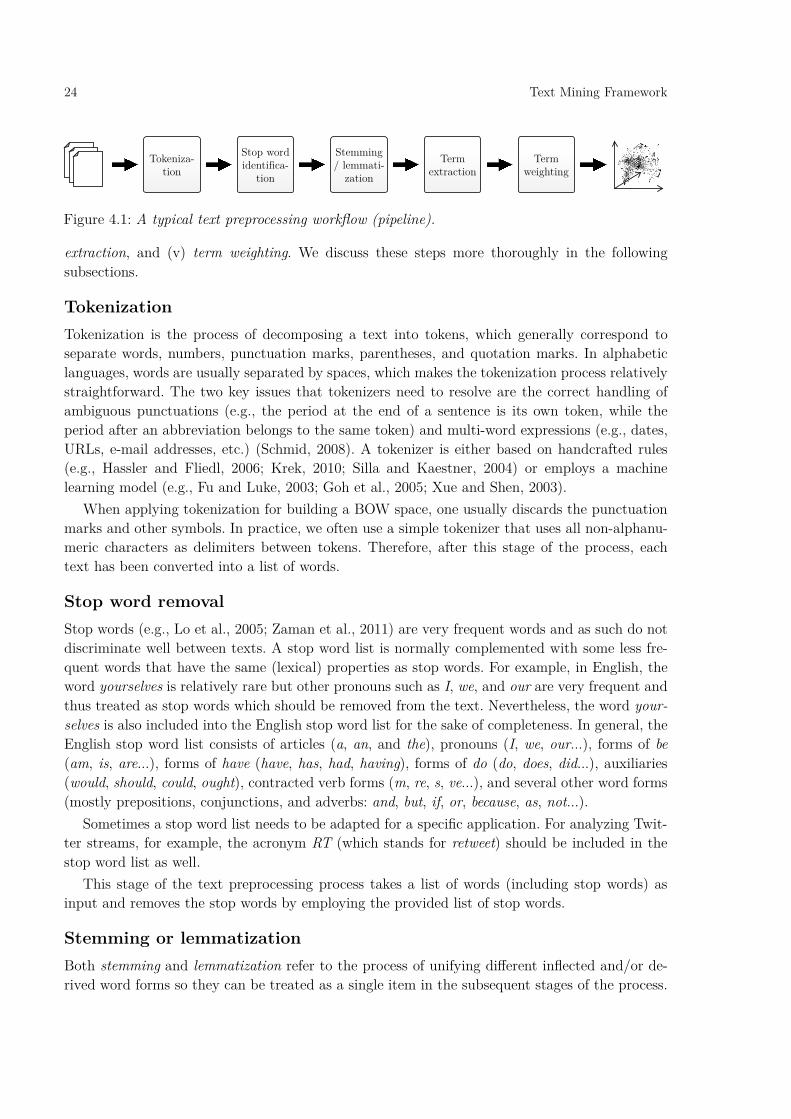
24 Text Mining Framework
extraction, and (v) term weighting. We discuss these steps more thoroughly in the following subsections.
Tokenization Tokenization is the process of decomposing a text into tokens, which generally correspond to separate words, numbers, punctuation marks, parentheses, and quotation marks. In alphabetic languages, words are usually separated by spaces, which makes the tokenization process relatively straightforward. The two key issues that tokenizers need to resolve are the correct handling of ambiguous punctuations (e.g., the period at the end of a sentence is its own token, while the period after an abbreviation belongs to the same token) and multi-word expressions (e.g., dates, URLs, e-mail addresses, etc.) (Schmid, 2008). A tokenizer is either based on handcrafted rules (e.g., Hassler and Fliedl, 2006; Krek, 2010; Silla and Kaestner, 2004) or employs a machine learning model (e.g., Fu and Luke, 2003; Goh et al., 2005; Xue and Shen, 2003).
When applying tokenization for building a BOW space, one usually discards the punctuation marks and other symbols. In practice, we often use a simple tokenizer that uses all non-alphanu-meric characters as delimiters between tokens. Therefore, after this stage of the process, each text has been converted into a list of words.
Stop word removal Stop words (e.g., Lo et al., 2005; Zaman et al., 2011) are very frequent words and as such do not discriminate well between texts. A stop word list is normally complemented with some less fre-quent words that have the same (lexical) properties as stop words. For example, in English, the word yourselves is relatively rare but other pronouns such as I, we, and our are very frequent and thus treated as stop words which should be removed from the text. Nevertheless, the word your-selves is also included into the English stop word list for the sake of completeness. In general, the English stop word list consists of articles (a, an, and the), pronouns (I, we, our...), forms of be (am, is, are...), forms of have (have, has, had, having), forms of do (do, does, did...), auxiliaries (would, should, could, ought), contracted verb forms (m, re, s, ve...), and several other word forms (mostly prepositions, conjunctions, and adverbs: and, but, if, or, because, as, not...).
Sometimes a stop word list needs to be adapted for a specific application. For analyzing Twit-ter streams, for example, the acronym RT (which stands for retweet) should be included in the stop word list as well.
This stage of the text preprocessing process takes a list of words (including stop words) as input and removes the stop words by employing the provided list of stop words.
Stemming or lemmatization Both stemming and lemmatization refer to the process of unifying different inflected and/or de-rived word forms so they can be treated as a single item in the subsequent stages of the process.
Figure 4.1: A typical text preprocessing workflow (pipeline).
Tokeniza-tion
Stop word identifica-
tion
Stemming / lemmati-
zation
Term extraction
Term weighting

Text Mining Framework 25
The purpose of this step is to reduce the dimensionality of the resulting BOW space and to establish explicit relationships between words with roughly the same meaning and lexical form.
Stemming refers to transforming a word into a stem which corresponds to the root of the word. The root of a word, in the strictest sense, is the primary lexical unit of the word which cannot be reduced into smaller constituents. It is obtained by stripping the word of all its inflectional and derivational affixes. For example, the root of the word friendships, in the strictest sense, is friend (in this case, -s is an inflectional suffix and -ship is a derivational suffix). However, stem-ming normally does not produce roots in the strictest sense but rather removes inflections and some (but not all) derivational suffixes. One of the most well-known stemmers for English is the Porter stemmer (Porter, 1980) which implements a set of rules for suffix stripping. By employing the Porter stemmer, the word friendships is transformed into friendship (rather than friend), so in this case, only the inflection is removed. On the other hand, the word connections is trans-formed into connect. In this case, not only the inflection -s but also the derivational suffix -ion are removed.
While there is no strict definition of what a stem is, other than being a lexical unit of a word with certain affixes removed, the lemma is the canonical form, dictionary form, or citation form of a set of words (sometimes also called a headword or catchword). It is the word under which a set of related dictionary or encyclopedia entries appear. Lemmatization thus refers to transform-ing a word into its base dictionary form. While a stemmer normally consists of a relatively simple set of rules for handling affixes, a lemmatizer needs to respect the conventions by which diction-aries are organized for a certain language. This makes its implementation more difficult. Lemma-tization algorithms are based on lexicons such as WordNet (Fellbaum, 1998; Miller, 1995), and on rules or models induced from language corpora by the use of machine learning (e.g., Juršič et al., 2010).
After this stage of text preprocessing, each text has been converted into a list of words where stop words have been removed, and each word in the list has been assigned its stem or lemma.
Term extraction Terminology extraction is normally a two-step process: (i) a linguistic processor is employed to extract typical terminological structures, and (ii) the resulting list of candidate terms is filtered according to various rules (Sclano and Velardi, 2007). When transforming texts into BOWs, a very simple term extractor is usually employed. It is based on a simple Apriori-like approach (Rakesh and Ramakrishnan, 1994) to discovering frequent (short) sequences of words (tokens) of length of 𝑛𝑛 words. Such sequences are called 𝑛𝑛-grams and are often used to complement the single words when constructing a BOW space (Cavnar and Trenkle, 1994).
The 𝑛𝑛 -gram extractor is configured with two important parameters: (i) maximum 𝑛𝑛 -gram length and (ii) minimum (required) term frequency. The first parameter determines the maximum length of terms (in the number of words) that should be extracted. The second parameter denotes the minimum number of times a particular stem or lemma needs to appear in the corpus so that the corresponding occurrences (in different forms) are annotated as terms. In the frequent-item-sets terminology, this is called “support”. If the minimum term frequency is set to greater than 1, the term extraction process can be optimized in terms of memory usage, which makes it applicable to extremely large corpora.
Technically, this step of the process converts a list of words, corresponding to a particular text in the corpus, into a list of terms. The single words are normally included in the resulting list

26 Text Mining Framework
and complemented with multi-word terms (e.g., bigrams and trigrams). A multi-word term nor-mally “inherits” the stems or lemmas from the words from which it was created.
Term weighting A term-weighting scheme defines how the components of a BOW vector are computed. In other words, it defines how a list of terms is converted into a BOW vector. Note that when we use the word “term” in this section, we in fact refer to a stem or lemma (unless neither stemming nor lemmatization was applied).
Let us denote the collection of preprocessed texts, produced by the term extraction step, with 𝐓𝐓′ = (𝐭𝐭1
′ , 𝐭𝐭2′ , … , 𝐭𝐭𝑚𝑚
′ ). Technically, each 𝐭𝐭𝑖𝑖′ can be viewed as a list of extracted terms. Suppose that
each unique term that can be found in 𝐓𝐓′ is mapped to a positive integer identifier between (and including) 1 and 𝑛𝑛 (𝑛𝑛 is the number of different terms in the corpus), so that no two different terms are assigned the same identifier. Let us now denote the BOW vector resulting from a particular text 𝐭𝐭𝑖𝑖
′ with 𝐱𝐱𝑖𝑖 = �𝑤𝑤𝑖𝑖,1, 𝑤𝑤𝑖𝑖,2, … , 𝑤𝑤𝑖𝑖,𝑛𝑛�. Here, 𝑤𝑤𝑖𝑖,𝑘𝑘 represents the weight of the term 𝑘𝑘. The weights 𝑤𝑤𝑖𝑖,𝑘𝑘 can be computed in several different ways, some of which are the following:
• Binary weights. A binary weight is either 0 or 1. It is computed according to the following simple rule: 𝑤𝑤𝑖𝑖,𝑘𝑘 is 1 if the term 𝑘𝑘 occurs in 𝐭𝐭𝑖𝑖
′. Otherwise, it is 0. • Term-frequency (TF) weights. A TF weight is simply the number of times the term 𝑘𝑘 occurs
in 𝐭𝐭𝑖𝑖′. Let us denote it with 𝑇𝑇𝑇𝑇𝑖𝑖,𝑘𝑘.
• TF-IDF weights (Salton, 1989). This is the most widely used weighting scheme in text mining. A TF-IDF weight is a combination of the TF value (see above) and IDF value, where IDF stands for inverse document frequency. IDF is computed as follows:
𝐼𝐼𝐼𝐼𝑇𝑇𝑘𝑘 = 𝑙𝑙𝑙𝑙𝑙𝑙 |𝐓𝐓′|𝑚𝑚𝑘𝑘
(?)
where 𝑚𝑚𝑘𝑘 is the number of texts in 𝐓𝐓′ that contain the term 𝑘𝑘. A TF-IDF weight is simply the TF weight multiplied by the IDF weight:
𝑇𝑇𝑇𝑇-𝐼𝐼𝐼𝐼𝑇𝑇𝑖𝑖,𝑘𝑘 = 𝑇𝑇𝑇𝑇𝑖𝑖,𝑘𝑘𝐼𝐼𝐼𝐼𝑇𝑇𝑘𝑘 (?)
A TF-IDF scheme weights a term higher if it occurs often in the same text (the TF com-ponent) and at the same time lower if it occurs in many texts from the corpus (the IDF component).
The output of this stage of the process depends on the setting in which the text preprocessing pipeline is employed. Normally, the pipeline constructs a BOW space and projects the initial text collection into this BOW space. It equips each dimension of the BOW space with (i) the infor-mation on the corresponding term (its stem or lemma and its most frequent form) and (ii) the IDF value corresponding to that term. In supervised learning (see Section 4.1.3), however, the preprocessing pipeline can also be used to project a text or a collection of texts into an existing BOW space. In this case, the information about the dimensions, including the set of IDF values, is adopted from this BOW space. The list of terms of a new text is thus filtered according to which terms are available in the existing BOW space. Furthermore, when computing TF-IDF weights, the IDF component for a particular term is not assessed from the new collection of documents but rather inherited from the original BOW space.
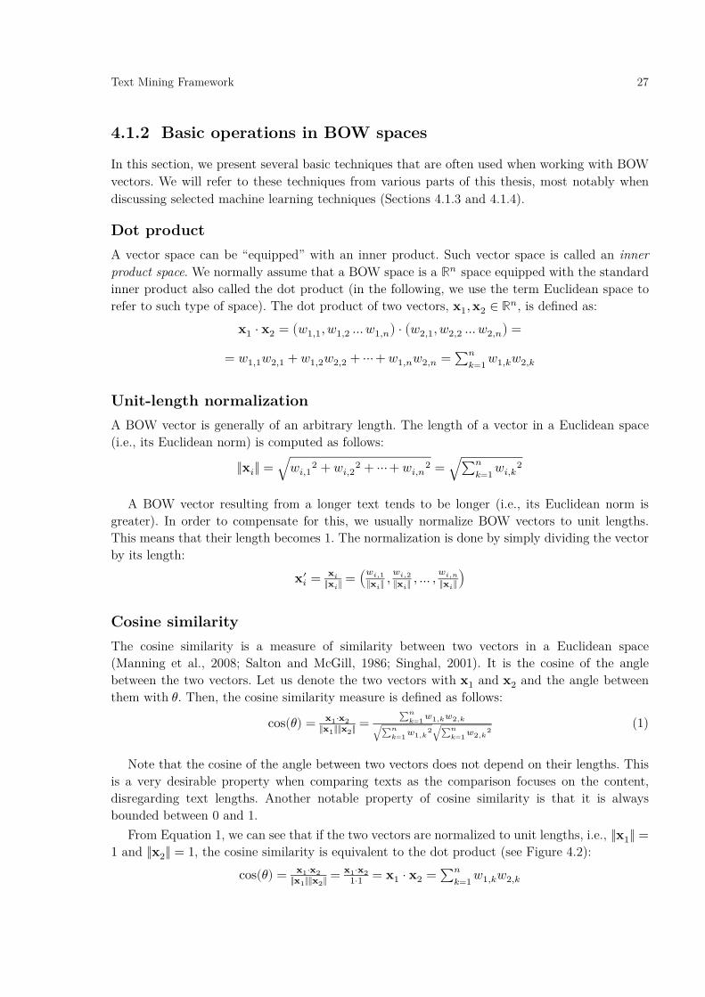
Text Mining Framework 27
4.1.2 Basic operations in BOW spaces
In this section, we present several basic techniques that are often used when working with BOW vectors. We will refer to these techniques from various parts of this thesis, most notably when discussing selected machine learning techniques (Sections 4.1.3 and 4.1.4).
Dot product A vector space can be “equipped” with an inner product. Such vector space is called an inner product space. We normally assume that a BOW space is a ℝ𝑛𝑛 space equipped with the standard inner product also called the dot product (in the following, we use the term Euclidean space to refer to such type of space). The dot product of two vectors, 𝐱𝐱1, 𝐱𝐱2 ∈ ℝ𝑛𝑛, is defined as:
𝐱𝐱1 · 𝐱𝐱2 = �𝑤𝑤1,1, 𝑤𝑤1,2 …𝑤𝑤1,𝑛𝑛� · �𝑤𝑤2,1, 𝑤𝑤2,2 …𝑤𝑤2,𝑛𝑛� = (?)
= 𝑤𝑤1,1𝑤𝑤2,1 + 𝑤𝑤1,2𝑤𝑤2,2 + ⋯ + 𝑤𝑤1,𝑛𝑛𝑤𝑤2,𝑛𝑛 = ∑ 𝑤𝑤1,𝑘𝑘𝑤𝑤2,𝑘𝑘𝑛𝑛𝑘𝑘=1 (?)
Unit-length normalization A BOW vector is generally of an arbitrary length. The length of a vector in a Euclidean space (i.e., its Euclidean norm) is computed as follows:
‖𝐱𝐱𝑖𝑖‖ = �𝑤𝑤𝑖𝑖,12 + 𝑤𝑤𝑖𝑖,2
2 + ⋯+ 𝑤𝑤𝑖𝑖,𝑛𝑛2 = �∑ 𝑤𝑤𝑖𝑖,𝑘𝑘
2𝑛𝑛𝑘𝑘=1 (?)
A BOW vector resulting from a longer text tends to be longer (i.e., its Euclidean norm is greater). In order to compensate for this, we usually normalize BOW vectors to unit lengths. This means that their length becomes 1. The normalization is done by simply dividing the vector by its length:
𝐱𝐱𝑖𝑖′ = 𝐱𝐱𝑖𝑖
‖𝐱𝐱𝑖𝑖‖= �𝑤𝑤𝑖𝑖,1
‖𝐱𝐱𝑖𝑖‖, 𝑤𝑤𝑖𝑖,2
‖𝐱𝐱𝑖𝑖‖,… , 𝑤𝑤𝑖𝑖,𝑛𝑛
‖𝐱𝐱𝑖𝑖‖� (?)
Cosine similarity The cosine similarity is a measure of similarity between two vectors in a Euclidean space (Manning et al., 2008; Salton and McGill, 1986; Singhal, 2001). It is the cosine of the angle between the two vectors. Let us denote the two vectors with 𝐱𝐱1 and 𝐱𝐱2 and the angle between them with 𝜃𝜃. Then, the cosine similarity measure is defined as follows:
cos(𝜃𝜃) = 𝐱𝐱1·𝐱𝐱2‖𝐱𝐱1‖‖𝐱𝐱2‖ = ∑ 𝑤𝑤1,𝑘𝑘𝑤𝑤2,𝑘𝑘
𝑛𝑛𝑘𝑘=1
�∑ 𝑤𝑤1,𝑘𝑘2𝑛𝑛
𝑘𝑘=1 �∑ 𝑤𝑤2,𝑘𝑘2𝑛𝑛
𝑘𝑘=1
(1)
Note that the cosine of the angle between two vectors does not depend on their lengths. This is a very desirable property when comparing texts as the comparison focuses on the content, disregarding text lengths. Another notable property of cosine similarity is that it is always bounded between 0 and 1.
From Equation 1, we can see that if the two vectors are normalized to unit lengths, i.e., ‖𝐱𝐱1‖ =1 and ‖𝐱𝐱2‖ = 1, the cosine similarity is equivalent to the dot product (see Figure 4.2):
cos(𝜃𝜃) = 𝐱𝐱1·𝐱𝐱2‖𝐱𝐱1‖‖𝐱𝐱2‖ = 𝐱𝐱1·𝐱𝐱2
1·1 = 𝐱𝐱1 · 𝐱𝐱2 = ∑ 𝑤𝑤1,𝑘𝑘𝑤𝑤2,𝑘𝑘𝑛𝑛𝑘𝑘=1 (?)

28 Text Mining Framework
Moreover, we can see that if any of 𝑤𝑤1,𝑘𝑘 and 𝑤𝑤2,𝑘𝑘 is 0, the corresponding product is also 0. These two observations can be turned into a recipe for a more efficient cosine similarity computation. First, BOW vectors should be normalized before provided as a dataset. This allows us to use dot product instead of cosine similarity and achieve the same results without the need to compute vector lengths. Secondly, when computing a dot product, only the overlapping non-zero values need to be considered. Due to the fact that BOW vectors are normally highly sparse, the number of such values is relatively low.
Centroids Intuitively, the term centroid refers to the gravitational point (or the average point) of a set of points in a Euclidean space (Han and Karypis, 2000). In a ℝ𝑛𝑛 vector space, the endpoints (heads, tips) of the vectors correspond to these points.
Let us denote a collection of vectors with 𝐂𝐂 = {𝐱𝐱1,… , 𝐱𝐱𝑛𝑛}. The centroid of this collection of vectors in a vector space is computed as follows:
𝑐𝑐(𝐂𝐂) = 1|𝐂𝐂| ∑ 𝐱𝐱𝑖𝑖𝐱𝐱𝑖𝑖∈𝐂𝐂 (?)
As noted earlier, we usually normalize BOW vectors in order to speed up the similarity com-putation process. The endpoints of such normalized vectors always lie on a hyper-sphere with radius 1 and in the part of the space with non-negative coordinates. A centroid is expected to have this same property in order to be compatible with BOW vectors. For this reason, we usually normalize BOW centroids:
𝑐𝑐(̂𝐂𝐂) = 𝑐𝑐(𝐂𝐂)‖𝑐𝑐(𝐂𝐂)‖ =
∑ 𝐱𝐱𝑖𝑖𝐱𝐱𝑖𝑖∈𝐂𝐂
�∑ 𝐱𝐱𝑖𝑖𝐱𝐱𝑖𝑖∈𝐂𝐂 � (2)
Figure 4.2: The cosine similarity measure. The figure shows two vectors, 𝐱𝐱1 and 𝐱𝐱2, and the corresponding two normalized representations, 𝐱𝐱1
′ and 𝐱𝐱2′ . The cosine similarity (i.e., the cosine
of the angle 𝜃𝜃) between 𝐱𝐱1 and 𝐱𝐱2 is equivalent to the dot product of 𝐱𝐱1′ and 𝐱𝐱2
′ .
x1
x2
0
1x1'
x2'
θ
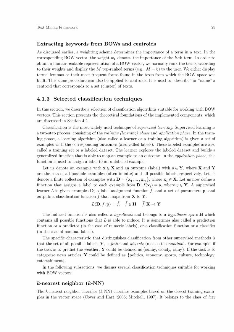
Text Mining Framework 29
Extracting keywords from BOWs and centroids As discussed earlier, a weighting scheme determines the importance of a term in a text. In the corresponding BOW vector, the weight 𝑤𝑤𝑘𝑘 denotes the importance of the 𝑘𝑘-th term. In order to obtain a human-readable representation of a BOW vector, we normally rank the terms according to their weights and display the 𝑀𝑀 top-ranked terms (e.g., 𝑀𝑀 = 5) to the user. We either display terms’ lemmas or their most frequent forms found in the texts from which the BOW space was built. This same procedure can also be applied to centroids. It is used to “describe” or “name” a centroid that corresponds to a set (cluster) of texts.
4.1.3 Selected classification techniques
In this section, we describe a selection of classification algorithms suitable for working with BOW vectors. This section presents the theoretical foundations of the implemented components, which are discussed in Section 4.2.
Classification is the most widely used technique of supervised learning. Supervised learning is a two-step process, consisting of the training (learning) phase and application phase. In the train-ing phase, a learning algorithm (also called a learner or a training algorithm) is given a set of examples with the corresponding outcomes (also called labels). These labeled examples are also called a training set or a labeled dataset. The learner explores the labeled dataset and builds a generalized function that is able to map an example to an outcome. In the application phase, this function is used to assign a label to an unlabeled example.
Let us denote an example with 𝐱𝐱 ∈ 𝐗𝐗 and an outcome (label) with 𝑦𝑦 ∈ 𝐘𝐘, where 𝐗𝐗 and 𝐘𝐘 are the sets of all possible examples (often infinite) and all possible labels, respectively. Let us denote a finite collection of examples with 𝐃𝐃 = {𝐱𝐱1,… , 𝐱𝐱𝑚𝑚}, where 𝐱𝐱𝑖𝑖 ∈ 𝐗𝐗. Let us now define a function that assigns a label to each example from 𝐃𝐃: 𝑓𝑓(𝐱𝐱𝑖𝑖) = 𝑦𝑦, where 𝑦𝑦 ∈ 𝐘𝐘. A supervised learner 𝐿𝐿 is given examples 𝐃𝐃, a label-assignment function 𝑓𝑓 , and a set of parameters 𝐩𝐩, and outputs a classification function 𝑓𝑓 ̂that maps from 𝐗𝐗 to 𝐘𝐘:
𝐿𝐿(𝐃𝐃, 𝑓𝑓, 𝐩𝐩) = 𝑓𝑓,̂ 𝑓𝑓 ̂∈ 𝐇𝐇, 𝑓𝑓 :̂𝐗𝐗 → 𝐘𝐘 (?)
The induced function is also called a hypothesis and belongs to a hypothesis space 𝐇𝐇 which contains all possible functions that 𝐿𝐿 is able to induce. It is sometimes also called a prediction function or a predictor (in the case of numeric labels), or a classification function or a classifier (in the case of nominal labels).
The specific characteristic that distinguishes classification from other supervised methods is that the set of all possible labels, 𝐘𝐘, is finite and discrete (most often nominal). For example, if the task is to predict the weather, 𝐘𝐘 could be defined as {sunny, cloudy, rainy}. If the task is to categorize news articles, 𝐘𝐘 could be defined as {politics, economy, sports, culture, technology, entertainment}.
In the following subsections, we discuss several classification techniques suitable for working with BOW vectors.
𝒌𝒌-nearest neighbor (𝒌𝒌-NN) The 𝑘𝑘-nearest neighbor classifier (𝑘𝑘-NN) classifies examples based on the closest training exam-ples in the vector space (Cover and Hart, 2006; Mitchell, 1997). It belongs to the class of lazy

30 Text Mining Framework
learners because it does not build a model in the training phase. Instead, it explores the training set in the classification phase and performs the following steps:
1. Find 𝑘𝑘 labeled examples most similar to the unlabeled example (according to a similarity measure 𝑠𝑠). Let us denote the 𝑘𝑘 nearest neighbors with 𝐍𝐍 = {𝐧𝐧1,… , 𝐧𝐧𝑘𝑘}.
2. Explore the labels of these 𝑘𝑘 labeled examples and count the number of times each partic-ular label occurs.
3. Classify the unlabeled example into the class corresponding to the label with the largest count. This can be formally written as follows:
𝑓𝑓(̂𝐱𝐱) = argmax𝑦𝑦∈𝐘𝐘 ∑ 𝛿𝛿�𝑦𝑦, 𝑓𝑓(𝐧𝐧𝑖𝑖)�𝑘𝑘𝑖𝑖=1 (?)
where 𝛿𝛿(𝑎𝑎, 𝑏𝑏) = 1 if 𝑎𝑎 = 𝑏𝑏 and 0 otherwise. A slightly modified 𝑘𝑘-NN algorithm also incorporates similarity scores into the target class
computation. Such algorithm is called the similarity-weighted nearest neighbor algorithm. The classification is performed in the following way:
𝑓𝑓(̂𝐱𝐱) = argmax𝑦𝑦∈𝐘𝐘 ∑ 𝑠𝑠(𝐱𝐱, 𝐧𝐧𝑖𝑖)𝛿𝛿�𝑦𝑦, 𝑓𝑓(𝐧𝐧𝑖𝑖)�𝑘𝑘𝑖𝑖=1 (?)
where 𝑠𝑠 denotes a similarity measure. In a BOW-based text-mining setting, 𝑠𝑠 normally corre-sponds to cosine similarity.
Nearest centroid classifier The nearest centroid classifier or nearest prototype classifier classifies an example into the class with the nearest centroid (Han and Karypis, 2000).
Let us denote the set of training examples that correspond to the label 𝑦𝑦 ∈ 𝐘𝐘 with 𝐃𝐃𝑦𝑦 ={𝐱𝐱𝑖𝑖: 𝑖𝑖 ∈ 1. . 𝑚𝑚, 𝑓𝑓(𝐱𝐱𝑖𝑖) = 𝑦𝑦}. Let us further denote the normalized centroid vector computed from 𝐃𝐃𝑦𝑦, according to Equation 2, with 𝑐𝑐(𝐃𝐃𝑦𝑦). The nearest centroid classifier is relatively straightfor-ward. In the training phase, it computes a centroid 𝑐𝑐(𝐃𝐃𝑦𝑦) for each class 𝑦𝑦. In the classification phase, it classifies a test example 𝐱𝐱 into the class with the nearest centroid according to the following equation:
𝑓𝑓(̂𝐱𝐱) = argmax𝑦𝑦∈𝐘𝐘{𝑠𝑠�𝐱𝐱, 𝑐𝑐(𝐃𝐃𝑦𝑦)�} (?)
where s is a similarity measure. In a BOW-based text-mining setting, 𝑠𝑠 normally corresponds to cosine similarity. When applied to BOW vectors, the nearest centroid classifier is extremely effi-cient and tends to be highly accurate.
Support vector machine (SVM) In general, support vector machine (SVM) refers to a family of kernel methods for supervised learning. The most widely used algorithm is the SVM classifier, which is often simply referred to as SVM (Joachims, 1998, 1999, 2002; Vapnik, 1995). SVM is a binary classifier, which means that it can map an unlabeled input example to one of two classes often referred to as the positive and negative class. In the training phase, the SVM learner constructs a hyperplane (i.e., a plane in a high-dimensional space), which separates positive from negative examples.
A hyperplane in a Euclidean space can be written as 𝐰𝐰 ⋅ 𝐱𝐱 − 𝑏𝑏 = 0, where 𝐰𝐰 is the normal vector to the hyperplane and 𝑏𝑏 denotes the hyperplane bias (𝑏𝑏 ‖𝐰𝐰‖⁄ is the distance from the hy-perplane to the origin in the direction of 𝐰𝐰). In the original SVM formulation, the hyperplane is

Text Mining Framework 31
positioned by maximizing the margin around it under the constraint that no example lies within the margin. The margin boundaries are defined as 𝐰𝐰 ⋅ 𝐱𝐱 − 𝑏𝑏 = 1 and 𝐰𝐰 ⋅ 𝐱𝐱 − 𝑏𝑏 = −1. The width of such margin is 2 ‖𝐰𝐰‖⁄ , which means that if we want to maximize the margin, we need to minimize ‖𝐰𝐰‖. The SVM problem can thus be formulated as follows:
Find 𝒘𝒘 and 𝑏𝑏 which minimize ‖𝒘𝒘‖ and in addition, for any 𝒙𝒙𝑖𝑖 from the training set, the following condition holds:
𝑦𝑦𝑖𝑖(𝐰𝐰 ⋅ 𝐱𝐱𝑖𝑖 − 𝑏𝑏) ≥ 1 (?)
where yi is the label of xi and is 1 for positive examples and −1 for negative examples. This condition basically states that every xi needs to lie outside or on the boundary of the margin.
Since not every dataset is perfectly linearly separable and thus the above optimization problem does not have a solution, the SVM problem can be reformulated so that it has a solution even if some training examples are misclassified or lie within the margin. It is based on the idea of soft margin where each example that is either misclassified or lies within the margin is penalized in the optimization function. We introduce a non-negative slack variable ξ𝑖𝑖 for each example 𝐱𝐱𝑖𝑖. If ξ𝑖𝑖 is positive, 𝐱𝐱𝑖𝑖 either lies on the correct side of the hyperplane but within the margin or it lies on the incorrect side of the hyperplane (i.e., is misclassified). The distance between such 𝐱𝐱𝑖𝑖 and the margin boundary on the correct side of the hyperplane is ξ𝑖𝑖 ‖𝐰𝐰‖⁄ . We want to minimize the sum of ξ𝑖𝑖 and at the same time maximize the margin. Since these two conditions are contradictory, we introduce the trade-off parameter 𝐶𝐶 which allows us to control which of the two conditions has a larger influence in the optimization function. The soft-margin problem is formulated as follows:
Find 𝒘𝒘, 𝑏𝑏, and (consequently) ξ𝑖𝑖 which minimize 12 ‖𝒘𝒘‖2 + 𝐶𝐶 ∑ ξ𝑖𝑖𝑖𝑖 and in addition, for any 𝒙𝒙𝑖𝑖 from the training set, the following condition holds:
𝑦𝑦𝑖𝑖(𝐰𝐰 ⋅ 𝐱𝐱𝑖𝑖 − 𝑏𝑏) ≥ 1 − ξ𝑖𝑖, ξ𝑖𝑖 ≥ 0 (?)
If 𝐱𝐱𝑖𝑖 lies outside the margin or on the boundary, then ξ𝑖𝑖 = 0. If it lies on the correct side of the hyperplane but within the margin, then 0 < ξ𝑖𝑖 < 1. If it lies on the hyperplane, then ξ𝑖𝑖 = 1. If it lies on the incorrect side of the hyperplane, then ξ𝑖𝑖 > 1.
In the classification phase, an unlabeled example 𝐱𝐱 is classified according to its position with respect to the hyperplane. If it lies on the positive side of the hyperplane, it is labeled as positive and if it lies on the negative side, as negative. If it lies directly on the hyperplane, its label cannot be determined. In general, the SVM classifier returns a score that is proportional to the distance between the unlabeled (test) example and the hyperplane:
𝑐𝑐(𝐱𝐱) = 𝐰𝐰 ⋅ 𝐱𝐱 − 𝑏𝑏 (?)
𝑓𝑓(̂𝐱𝐱) = sgn�𝑐𝑐(𝐱𝐱)� (?)
The Euclidean distance between 𝐱𝐱 and the hyperplane (in the direction of 𝐰𝐰) is 𝑐𝑐(𝐱𝐱) ‖𝐰𝐰‖⁄ . The SVM optimization problem can be rewritten into a form that can be solved by standard
quadratic programming techniques. This formulation reveals that the resulting hyperplane can be defined as a linear combination of training examples. In this combination, only a relatively
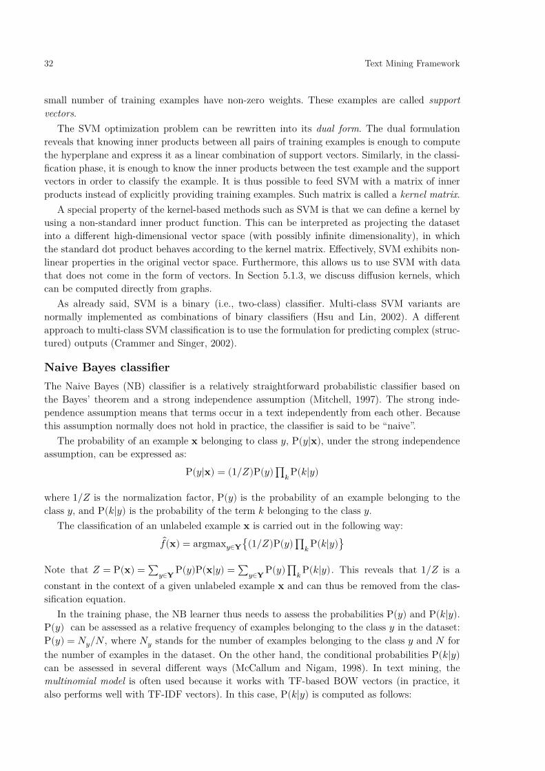
32 Text Mining Framework
small number of training examples have non-zero weights. These examples are called support vectors.
The SVM optimization problem can be rewritten into its dual form. The dual formulation reveals that knowing inner products between all pairs of training examples is enough to compute the hyperplane and express it as a linear combination of support vectors. Similarly, in the classi-fication phase, it is enough to know the inner products between the test example and the support vectors in order to classify the example. It is thus possible to feed SVM with a matrix of inner products instead of explicitly providing training examples. Such matrix is called a kernel matrix.
A special property of the kernel-based methods such as SVM is that we can define a kernel by using a non-standard inner product function. This can be interpreted as projecting the dataset into a different high-dimensional vector space (with possibly infinite dimensionality), in which the standard dot product behaves according to the kernel matrix. Effectively, SVM exhibits non-linear properties in the original vector space. Furthermore, this allows us to use SVM with data that does not come in the form of vectors. In Section 5.1.3, we discuss diffusion kernels, which can be computed directly from graphs.
As already said, SVM is a binary (i.e., two-class) classifier. Multi-class SVM variants are normally implemented as combinations of binary classifiers (Hsu and Lin, 2002). A different approach to multi-class SVM classification is to use the formulation for predicting complex (struc-tured) outputs (Crammer and Singer, 2002).
Naive Bayes classifier The Naive Bayes (NB) classifier is a relatively straightforward probabilistic classifier based on the Bayes’ theorem and a strong independence assumption (Mitchell, 1997). The strong inde-pendence assumption means that terms occur in a text independently from each other. Because this assumption normally does not hold in practice, the classifier is said to be “naive”.
The probability of an example 𝐱𝐱 belonging to class 𝑦𝑦, P(𝑦𝑦|𝐱𝐱), under the strong independence assumption, can be expressed as:
P(𝑦𝑦|𝐱𝐱) = (1 𝑍𝑍⁄ )P(𝑦𝑦)∏ P(𝑘𝑘|𝑦𝑦)𝑘𝑘 (?)
where 1/𝑍𝑍 is the normalization factor, P(𝑦𝑦) is the probability of an example belonging to the class 𝑦𝑦, and P(𝑘𝑘|𝑦𝑦) is the probability of the term 𝑘𝑘 belonging to the class 𝑦𝑦.
The classification of an unlabeled example 𝐱𝐱 is carried out in the following way:
𝑓𝑓(̂𝐱𝐱) = argmax𝑦𝑦∈𝐘𝐘�(1 𝑍𝑍⁄ )P(𝑦𝑦)∏ P(𝑘𝑘|𝑦𝑦)𝑘𝑘 � (?)
Note that 𝑍𝑍 = P(𝐱𝐱) = ∑ P(𝑦𝑦)P(𝐱𝐱|𝑦𝑦)𝑦𝑦∈𝐘𝐘 = ∑ P(𝑦𝑦)∏ P(𝑘𝑘|𝑦𝑦)𝑘𝑘𝑦𝑦∈𝐘𝐘 . This reveals that 1/𝑍𝑍 is a constant in the context of a given unlabeled example x and can thus be removed from the clas-sification equation.
In the training phase, the NB learner thus needs to assess the probabilities P(𝑦𝑦) and P(𝑘𝑘|𝑦𝑦). P(𝑦𝑦) can be assessed as a relative frequency of examples belonging to the class 𝑦𝑦 in the dataset: P(𝑦𝑦) = 𝑁𝑁𝑦𝑦/𝑁𝑁 , where 𝑁𝑁𝑦𝑦 stands for the number of examples belonging to the class 𝑦𝑦 and 𝑁𝑁 for the number of examples in the dataset. On the other hand, the conditional probabilities P(𝑘𝑘|𝑦𝑦) can be assessed in several different ways (McCallum and Nigam, 1998). In text mining, the multinomial model is often used because it works with TF-based BOW vectors (in practice, it also performs well with TF-IDF vectors). In this case, P(𝑘𝑘|𝑦𝑦) is computed as follows:

Text Mining Framework 33
P(𝑘𝑘|𝑦𝑦) = 𝑇𝑇𝑡𝑡𝑘𝑘,𝑦𝑦/𝑇𝑇𝑦𝑦 (?)
where 𝑇𝑇𝑡𝑡𝑘𝑘,𝑦𝑦 stands for the number of times the term 𝑡𝑡𝑘𝑘 occurs in the text that is the concatena-tion of all texts labeled as 𝑦𝑦 and 𝑇𝑇𝑦𝑦 stands for the length (in the number of words) of such concatenated text. Since 𝑇𝑇𝑡𝑡𝑘𝑘,𝑦𝑦 can be 0, which undesirably causes the entire expression P(𝑦𝑦)∏ P(𝑘𝑘|𝑦𝑦)𝑘𝑘 to be 0, a smoothed form of probability estimation such as the rule of succession or 𝑚𝑚-estimate (Cestnik, 1991) is normally used.
The factors in the expression ∏ P(𝑘𝑘|𝑦𝑦)𝑘𝑘 tend to be relatively small. Multiplying many small numbers together can result in an underflow. For this reason, the log-sum-exp trick can be used. By using the fact that 𝑎𝑎𝑏𝑏 = exp(log𝑎𝑎 + log𝑏𝑏), we can derive the following equations which are more robust to underflows:
P(𝑦𝑦|𝐱𝐱) = exp�(1/𝑍𝑍)logP(𝑦𝑦) + ∑ logP(𝑡𝑡𝑘𝑘|𝑦𝑦)𝑘𝑘 � (?)
𝑓𝑓(̂𝐱𝐱) = argmax𝑦𝑦∈𝐘𝐘�logP(𝑦𝑦)∑ logP(𝑘𝑘|𝑦𝑦)𝑘𝑘 � (?)
4.1.4 Selected clustering techniques
In this section, we describe two different clustering algorithms suitable for working with BOW vectors. This section presents the theoretical foundation of the implemented clustering compo-nents (the implemented components are discussed in Section 4.2).
In contrast to classification, clustering is a form of unsupervised learning. Unsupervised learn-ing refers to a set of methods that aim at finding a hidden structure in an unlabeled dataset. A clustering algorithm is given a set of unlabeled examples which it arranges into groups (i.e., clusters) so that the examples in the same group are more similar to each other than to those in the other groups.
Let us denote an unlabeled dataset with 𝐃𝐃 = {𝐱𝐱1,… ,𝐱𝐱𝑚𝑚}. A clustering algorithm 𝐶𝐶 is given an unlabeled dataset 𝐃𝐃 and a set of parameters 𝐩𝐩 and outputs a set of clusters:
𝐶𝐶(𝐃𝐃, 𝐩𝐩) = {𝐂𝐂1, 𝐂𝐂2,… , 𝐂𝐂𝑘𝑘} (3)
The output of a clustering algorithm can either be a flat list of clusters (as suggested by Equation 3) or a hierarchy of clusters. The number of clusters 𝑘𝑘 is normally specified in advance but can also be determined from the dataset (Pelleg and Moore, 2000). An example x𝑖𝑖 usually belongs to exactly one cluster, but clustering algorithms that allow the same example to belong to several clusters at the same time (potentially with different membership degrees) also exist (e.g., fuzzy 𝑐𝑐-means (Cannon et al., 1986)).
In general, the clustering algorithms can be divided into centroid-based algorithms (e.g., 𝑘𝑘-means), connectivity-based algorithms (e.g., agglomerative hierarchical clustering), distribution-based algorithms (e.g., Gaussian mixture models (Dempster et al., 1977)), or density-based algo-rithms (e.g., DBSCAN (Martin et al., 1996)).
𝒌𝒌-means clustering 𝑘𝑘-means clustering refers to a group of unsupervised methods aimed at partitioning a set of examples into 𝑘𝑘 groups (clusters). The most widely used algorithm is based on iterative refine-ment (Lloyd, 2006).

34 Text Mining Framework
The algorithm starts by randomly selecting 𝑘𝑘 examples as the initial centroids. Then, it enters the main loop in which it iteratively repeats two steps: assign and update. In the assign step, it assigns each example to the nearest centroid. In the update step, it recomputes the centroids. In this process, the centroids move around in the space. When they reach a local optimum, they stop moving and the main loop ends. More formally, the iterative 𝑘𝑘-means clustering algorithm is as follows:
Input: an unlabeled dataset of normalized BOW vectors 𝐃𝐃 = {𝐱𝐱1,… , 𝐱𝐱𝑚𝑚}
1. Initialization. Randomly select 𝑘𝑘 different examples from 𝐃𝐃. Let us denote these examples with 𝐳𝐳1,… , 𝐳𝐳𝑘𝑘. Create the initial clusters out of these examples 𝐂𝐂𝑖𝑖 ← {𝐳𝐳𝑖𝑖}, 𝑖𝑖 ∈ 1. . 𝑘𝑘, and compute their initial centroids 𝐜𝐜𝑖𝑖 ← 𝑐𝑐(𝐂𝐂𝑖𝑖) = 𝐳𝐳𝑖𝑖, 𝑖𝑖 ∈ 1. . 𝑘𝑘.
2. Assign step. For each example 𝐱𝐱𝑖𝑖, 𝑖𝑖 ∈ 1. . 𝑚𝑚, find the cluster 𝐂𝐂∗ with the most similar cen-troid:
𝐂𝐂∗ = argmax𝐂𝐂𝑗𝑗:𝑗𝑗∈1..𝑘𝑘{cossim�𝐜𝐜𝑗𝑗, 𝐱𝐱𝑖𝑖�} (*)
3. Add 𝐱𝐱𝑖𝑖 to this cluster: 𝐂𝐂∗ ← 𝐂𝐂∗ ∪ {𝐱𝐱𝑖𝑖} 4. Update step. Recompute the cluster centroids 𝐜𝐜𝑖𝑖 ← 𝑐𝑐(𝐂𝐂𝑖𝑖), 𝑖𝑖 ∈ 1. . 𝑘𝑘. The variable 𝐜𝐜𝑖𝑖 now
holds the centroid corresponding to the cluster 𝐂𝐂𝑖𝑖. 5. If the assignments did not change from the previous loop, end the algorithm. 6. Empty the clusters 𝐂𝐂𝑖𝑖 ← ∅, 𝑖𝑖 ∈ 1. . 𝑘𝑘. 7. Repeat from Step 2.
Output: Clusters 𝐂𝐂𝑖𝑖 and their centroids 𝐜𝐜𝑖𝑖, 𝑖𝑖 ∈ 1. . 𝑘𝑘.
Agglomerative hierarchical clustering Hierarchical clustering refers to a range of clustering algorithms that organize examples into a hierarchy of clusters (rather than a “flat” set of clusters). Agglomerative hierarchical clustering is a bottom-up approach, which means that at the beginning, each example represents a small cluster (Manning et al., 2008). These clusters then merge into bigger clusters at different levels of the hierarchy until there is only one cluster that contains all the examples (i.e., the root cluster).
Suppose that we have an unlabeled dataset of normalized BOW vectors 𝐃𝐃 = {𝐱𝐱1,… , 𝐱𝐱𝑚𝑚}. The agglomerative clustering process is as follows:
1. Initialization. Put each example into its own cluster 𝐂𝐂𝑖𝑖 = {𝐱𝐱𝑖𝑖}, 𝑖𝑖 ∈ 1. . 𝑚𝑚, and put these clusters into a list 𝐋𝐋 = {𝐂𝐂1,𝐂𝐂2, … , 𝐂𝐂𝑚𝑚}.
2. Main loop. Compute centroids corresponding to clusters 𝐂𝐂1,𝐂𝐂2, … , 𝐂𝐂𝑚𝑚. Put these cen-troids into a list 𝐋𝐋′ = {𝐜𝐜1, 𝐜𝐜2, … , 𝐜𝐜𝑚𝑚}.
3. Find the two most similar clusters 𝐂𝐂1∗ and 𝐂𝐂2
∗ :
(𝐂𝐂1∗,𝐂𝐂2
∗) = argmax�𝐂𝐂𝑖𝑖,𝐂𝐂𝑗𝑗�:𝐂𝐂𝑖𝑖∈𝐋𝐋,𝐂𝐂𝑗𝑗∈𝐋𝐋,𝑖𝑖≠𝑗𝑗{cossim�𝐜𝐜𝑖𝑖, 𝐜𝐜𝑗𝑗�} (*)
4. Merge the two clusters 𝐂𝐂∗ = 𝐂𝐂1∗ ∪ 𝐂𝐂2
∗ and compute the corresponding centroid 𝐜𝐜∗. 5. Remove 𝐂𝐂1
∗ and 𝐂𝐂2∗ from 𝐋𝐋. Add the new cluster 𝐂𝐂∗ to 𝐋𝐋. Also, at this point make note
that the cluster 𝐂𝐂∗ is the parent of the clusters 𝐂𝐂1∗ and 𝐂𝐂2
∗ in the resulting hierarchy. 6. Let 𝐜𝐜1
∗ and 𝐜𝐜2∗ bet the centroids corresponding to 𝐂𝐂1
∗ and 𝐂𝐂2∗ , respectively. Remove 𝐜𝐜1
∗ and 𝐜𝐜2
∗ from 𝐋𝐋′. Add the new centroid 𝐜𝐜∗ to 𝐋𝐋′. 7. If there is only one cluster in 𝐋𝐋, end the algorithm.

Text Mining Framework 35
8. Repeat from Step 3.
The algorithm is normally implemented by maintaining a (symmetric) matrix of centroid-centroid similarities. In Step 3, the algorithm thus avoids computing cosine similarity for each pair of centroids but rather explores the similarity matrix. The matrix is updated in Step 5, where the two rows and two columns corresponding to 𝐂𝐂1
∗ and 𝐂𝐂2∗ are removed from the matrix and a new
row and column, representing the new cluster 𝐂𝐂∗, are added. In this process, only the values cossim(𝐜𝐜∗, 𝐜𝐜𝑖𝑖), for each 𝐜𝐜𝑖𝑖 ∈ 𝐋𝐋′, need to be computed, which makes the described algorithm more efficient.
4.2 Implementation of selected text mining techniques in the ClowdFlows platform
The described text mining background technologies are implemented as part of this thesis in a text mining framework called LATINO. LATINO stands for Link Analysis and Text Mining Toolbox and is primarily a light-weight framework for building text mining applications. A large part of LATINO text mining functionality has been made available also in ClowdFlows, a web-based platform for composing and executing data mining workflows by means of visual program-ming (Kranjc et al., 2012).
In this section, we present the developed LATINO components which are available in Clowd-Flows. We first discuss the text preprocessing workflows which are used for representing texts as BOW vectors. Later on, we also discuss several workflows for performing classification and clus-tering in BOW spaces.
A prototypical ClowdFlows component is shown in Figure 4.3. It has a name (Dummy), input stubs (in1, in2) through which it receives (consumes) data, and output stubs (out1, out2) through which it sends (outputs, emits) data. It also has a configuration panel where the user is able to reconfigure the default behavior of the component. With respect to how a component behaves in a workflow, we distinguish between the following types of components: Data sources A data source is a component that “produces” data (datasets, models, reports...)
by, for example, loading it from a file or a database. It normally does not have input stubs and is triggered when the workflow is started. LATINO implements several data sources that produce annotated document corpora (ADCs). Specifically, it implements a component for loading an ADC from an XML file, from a simple plain text file (containing one text per line), from a collection of text files, etc.
Data sinks A data sink is a component that normally does not have any output stubs. It “consumes” data by either storing it or visualizing it to the user. LATINO currently imple-ments a sink for storing an ADC into an XML file and a sink for displaying an ADC as a set of HTML pages.
Hubs A hub is a component that executes a processing component but by itself does not perform any (data) processing. For example, a Tokenizer Hub receives an ADC, executes one of the tokenizers, and outputs the ADC with additional annotations corresponding to tokens. The component that a hub executes is attached to one of the hub’s input stubs. The existence of hubs is motivated by the following two reasons:
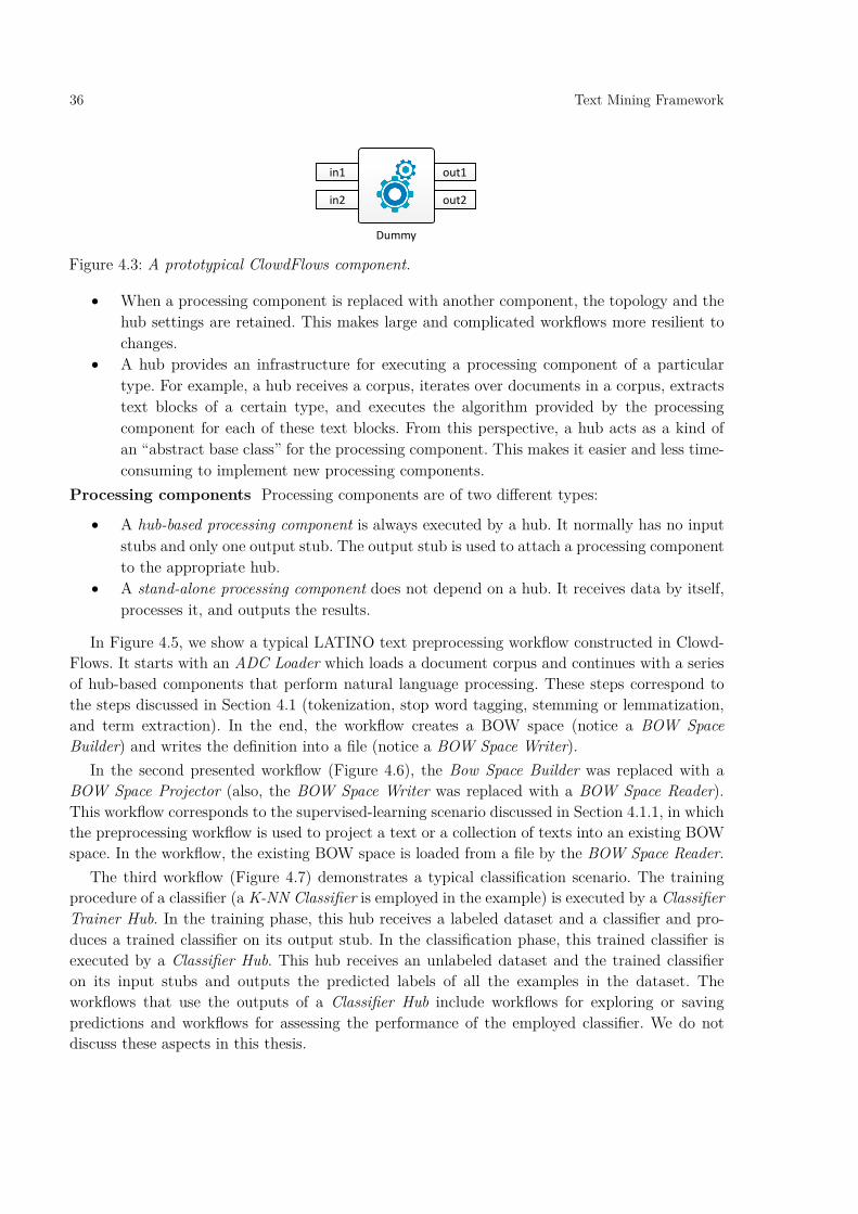
36 Text Mining Framework
• When a processing component is replaced with another component, the topology and the hub settings are retained. This makes large and complicated workflows more resilient to changes.
• A hub provides an infrastructure for executing a processing component of a particular type. For example, a hub receives a corpus, iterates over documents in a corpus, extracts text blocks of a certain type, and executes the algorithm provided by the processing component for each of these text blocks. From this perspective, a hub acts as a kind of an “abstract base class” for the processing component. This makes it easier and less time-consuming to implement new processing components.
Processing components Processing components are of two different types:
• A hub-based processing component is always executed by a hub. It normally has no input stubs and only one output stub. The output stub is used to attach a processing component to the appropriate hub.
• A stand-alone processing component does not depend on a hub. It receives data by itself, processes it, and outputs the results.
In Figure 4.5, we show a typical LATINO text preprocessing workflow constructed in Clowd-Flows. It starts with an ADC Loader which loads a document corpus and continues with a series of hub-based components that perform natural language processing. These steps correspond to the steps discussed in Section 4.1 (tokenization, stop word tagging, stemming or lemmatization, and term extraction). In the end, the workflow creates a BOW space (notice a BOW Space Builder) and writes the definition into a file (notice a BOW Space Writer).
In the second presented workflow (Figure 4.6), the Bow Space Builder was replaced with a BOW Space Projector (also, the BOW Space Writer was replaced with a BOW Space Reader). This workflow corresponds to the supervised-learning scenario discussed in Section 4.1.1, in which the preprocessing workflow is used to project a text or a collection of texts into an existing BOW space. In the workflow, the existing BOW space is loaded from a file by the BOW Space Reader.
The third workflow (Figure 4.7) demonstrates a typical classification scenario. The training procedure of a classifier (a K-NN Classifier is employed in the example) is executed by a Classifier Trainer Hub. In the training phase, this hub receives a labeled dataset and a classifier and pro-duces a trained classifier on its output stub. In the classification phase, this trained classifier is executed by a Classifier Hub. This hub receives an unlabeled dataset and the trained classifier on its input stubs and outputs the predicted labels of all the examples in the dataset. The workflows that use the outputs of a Classifier Hub include workflows for exploring or saving predictions and workflows for assessing the performance of the employed classifier. We do not discuss these aspects in this thesis.
Figure 4.3: A prototypical ClowdFlows component.
out1in1
in2 out2
Dummy

Text Mining Framework 37
The last workflow that we discuss (given in Figure 4.8), demonstrates a typical clustering scenario. The workflow is relatively straightforward. A Clusterer Hub receives a clustering algo-rithm (in our case, a K-Means Clusterer) and produces a set of clusters on the output stub. The workflows that use the output from a Clusterer Hub mainly include workflows for visualizing, exploring, or saving the clustering results. We do not present these workflows in this thesis.
In the following text, we discuss the components used in the presented workflows. In some situations, when a component is executed through a hub, we also present several alternatives to that particular component.
ADC Loader A LATINO text mining process starts with loading or creating an annotated document corpus (ADC). In short, an ADC contains one or more documents and is described with features. A document itself is also described with features and in addition contains (named) annotations. An annotation gives either a syntactic or a semantic meaning to a text segment (e.g., a text segment can represent token, sentence, named entity). An annotation can further be described with fea-tures.
An ADC can be represented in an XML format. This allows us to save and load it to/from a file. It also enables us to manually edit ADCs but it is often more convenient to do this in a programming environment through the ADC interface. An ADC can also be serialized into a set of HTML pages for viewing and exploration. This allows us to understand and improve the preprocessing stage of a text mining workflow. Figure 4.4 shows a document rendered as an HTML page.
The basic idea of using ADCs is that after an ADC has been loaded or somehow otherwise created, each subsequent component in the text-preprocessing part of the workflow receives this ADC as an input, adds additional annotations and/or features, and provides it as an output. For
Figure 4.4: An annotated document represented as HTML.
Figure 4.5: LATINO text preprocessing workflow (building a new BOW space).
ADC Loader Tokenizer Hub
Simple Tokenizer
Stop Word Tagger Hub
Stemmer/Lemmatizer Hub
Term Extractor Hub BOW Space Builder
DefaultStop Word Tagger
Lemmatizer(LemmaGen)
N-Gram Extractor
bow
BOW Space Writer
adc adcadc
tkn
tkn
adcadc
tgradc
adc
tgradc
adc
texadc
ds
tgr tgr tex
bow
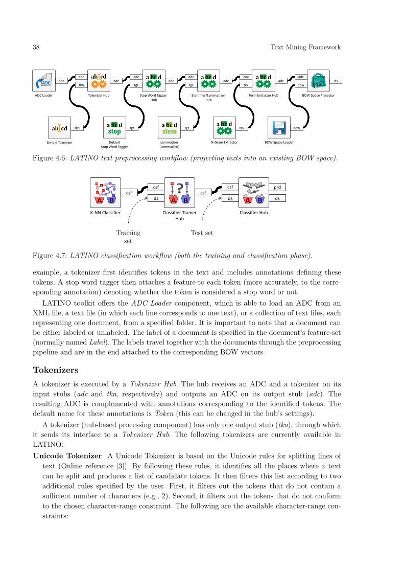
38 Text Mining Framework
example, a tokenizer first identifies tokens in the text and includes annotations defining these tokens. A stop word tagger then attaches a feature to each token (more accurately, to the corre-sponding annotation) denoting whether the token is considered a stop word or not.
LATINO toolkit offers the ADC Loader component, which is able to load an ADC from an XML file, a text file (in which each line corresponds to one text), or a collection of text files, each representing one document, from a specified folder. It is important to note that a document can be either labeled or unlabeled. The label of a document is specified in the document’s feature-set (normally named Label). The labels travel together with the documents through the preprocessing pipeline and are in the end attached to the corresponding BOW vectors.
Tokenizers A tokenizer is executed by a Tokenizer Hub. The hub receives an ADC and a tokenizer on its input stubs (adc and tkn, respectively) and outputs an ADC on its output stub (adc). The resulting ADC is complemented with annotations corresponding to the identified tokens. The default name for these annotations is Token (this can be changed in the hub’s settings).
A tokenizer (hub-based processing component) has only one output stub (tkn), through which it sends its interface to a Tokenizer Hub. The following tokenizers are currently available in LATINO: Unicode Tokenizer A Unicode Tokenizer is based on the Unicode rules for splitting lines of
text (Online reference [3]). By following these rules, it identifies all the places where a text can be split and produces a list of candidate tokens. It then filters this list according to two additional rules specified by the user. First, it filters out the tokens that do not contain a sufficient number of characters (e.g., 2). Second, it filters out the tokens that do not conform to the chosen character-range constraint. The following are the available character-range con-straints:
Figure 4.6: LATINO text preprocessing workflow (projecting texts into an existing BOW space).
Figure 4.7: LATINO classification workflow (both the training and classification phase).
ADC Loader Tokenizer Hub
Simple Tokenizer
Stop Word Tagger Hub
Stemmer/Lemmatizer Hub
Term Extractor Hub BOW Space Projector
DefaultStop Word Tagger
Lemmatizer(LemmaGen)
N-Gram Extractor BOW Space Loader
adc adcadc
tkn
tkn
adcadc
tgradc
adc
tgradc
adc
tex
tgr tgr tex
adc
bowds
bow
K-NN Classifier Classifier TrainerHub
Classifier Hub
csf csfcsf
ds
csf
ds
prd
ds
Training set
Test set

Text Mining Framework 39
• None. Accept all tokens. • AplphaNumLoose. Accept all the tokens that contain at least one alphanumeric character. • AlphaNumStrict. Accept all the tokens that contain only alphanumeric characters. • AlphaLoose. Accept all the tokens that contain at least one alphabetic character. • AlphaStrict. Accept all the tokens that contain only alphabetic characters.
Regex Tokenizer This tokenizer is configured with a single regular expression. It then traverses a text and finds all substrings that match the regular expressions. These matches correspond to the resulting tokens. By default, the regular expression is set to \p{L}{2,}, which means that all substrings of length at least 2 and containing only alphabetic characters will be iden-tified as tokens.
Simple Tokenizer The simple tokenizer implements three different modes:
• Default. In this mode, the tokenizer simply splits a text on every whitespace or series of whitespaces.
• Alphabetic. In the alphabetic mode, the tokenizer splits a text on every non-alphabetic character or series of non-alphabetic characters.
• Alphanumeric. In the alphanumeric mode, the tokenizer splits a text on every non-alpha-numeric character or series of non-alphanumeric characters.
Maximum Entropy Tokenizer This is the most sophisticated tokenizer currently included in the LATINO toolkit. It employs a maximum entropy model to detect boundaries between tokens in English texts. This tokenizer was originally developed in the open source project SharpNLP (Online reference [4]).
Stop word taggers A stop word tagger is executed by a Stop Word Tagger Hub. The hub receives an ADC and a tagger on its input stubs (adc and tgr, respectively) and outputs an ADC on its output stub (adc). In the resulting ADC, the annotations corresponding to tokens are complemented with an additional feature (named StopWord by default) which is either set to true or false.
A stop word tagger (hub-based processing component) has only one output stub (tgr), through which it sends its interface to a Stop Word Tagger Hub. LATINO currently implements only one stop word tagger, the Default Stop Word Tagger. This stop word tagger contains a set of stop word lists, one list for each supported language. It traverses the tokens in an ADC and identifies (marks) stop words according to the selected stop word list.
Most of the stop word lists used by this component were developed in the Snowball project (Online reference [5]). The following languages are currently supported: Bulgarian, Czech, Danish,
Figure 4.8: LATINO clustering workflow.
K-Means Clusterer Clusterer Hub
cls crcls
ds
Unlabeled dataset
40 Text Mining Framework
Dutch, English, Finnish, French, German, Hungarian, Italian, Norwegian, Portuguese, Romanian, Russian, Serbian, Slovene, Spanish, and Swedish. The component also allows the user to extend an existing list by loading or manually entering additional stop words.
Stemmers and lemmatizers A stemmer or lemmatizer is executed by a Stemmer/Lemmatizer Hub. The hub receives an ADC and a stemmer or lemmatizer on its input stubs (adc and tgr, respectively) and outputs an ADC on its output stub (adc). In the resulting ADC, the annotations corresponding to tokens are complemented with an additional feature (named Stem by default) containing the token’s stem or lemma. A stemmer or lemmatizer (hub-based processing component) has only one output stub (tgr), through which it sends its interface to a Stemmer/Lemmatizer Hub.
LATINO makes use of two open source projects for stemming and lemmatization. The first one is Snowball (Online reference [5]) which implements a set of stemmers. We use the C# port of Snowball provided in the scope of the Lucene.Net project (Online reference [6]). The Snowball stemmers are based on manually defined (Porter-like) rules for affix stripping. The second open source project is LemmaGen, a software library for lemmatization, implemented in C# (Online reference [7]). The LemmaGen lemmatizers are based on ripple-down rules (RDR) induced from gold-standard language corpora by employing machine learning.
The component that embodies the Snowball stemmers is called the Snowball Stemmer. It can be configured to use the stemming algorithm for a particular language. The following languages are currently supported: Danish, Dutch, English, Finnish, French, German, Italian, Norwegian, Portuguese, Russian, Spanish, and Swedish.
The functionality of LemmaGen, on the other hand, is provided by the LemmaGen Lemmatizer component. Likewise, it can be configured to use the lemmatization model for a particular lan-guage. The following languages are currently supported: Bulgarian, Czech, English, Estonian, French, German, Hungarian, Italian, Romanian, Serbian, Slovene, and Spanish.
Term extractors A term extractor is executed by a Term Extractor Hub. The hub receives an ADC and a term extractor on its input stubs (adc and tex, respectively) and outputs an ADC on its output stub (adc). The resulting ADC is complemented with annotations corresponding to the identified terms. The default name for these annotations is Term (this can be changed in the hub’s settings).
A term extractor, which is a hub-based processing component, has only one output stub (tex), through which it sends its interface to a Term Extractor Hub. LATINO currently implements only one component for term extraction, the N-Gram Term Extractor. It is based on a simple Apriori-like approach to discovering (frequent) sequences of words (tokens) of length of at most 𝑛𝑛 words. Such sequences are called 𝑛𝑛-grams and are often used to complement the single words when constructing a BOW space. An N-Gram Term Extractor is configured with two parameters: (i) maximum 𝑛𝑛-gram length and (ii) minimum (required) term frequency. The first parameter determines the maximum length of terms that should be extracted. The second parameter defines the support for discovering frequent sequences.
BOW Space Builder The BOW Space Builder component is a stand-alone processing component. It receives an ADC through its input stub (adc) and outputs two objects: (i) the definition of the corresponding
Text Mining Framework 41
BOW space (output stub bow) and (ii) the BOW representations of the input texts in the form of an unlabeled dataset (output stub ds).
A BOW Space Builder is configured with three parameters. The first one is the term weighting scheme. It can be either set to binary, Term Frequency, or TF-IDF. The second parameter, the cut-off parameter, allows us to cut off the tails of BOW vectors. Finally, the third parameter allows us to set whether to normalize the resulting vectors or not. If set to true, the BOW Space Builder produces a dataset in which each BOW vector is normalized to the unit length.
BOW Space Writer and BOW Space Reader A BOW space is in its essence a LATINO object. It can serialize itself to a stream of bytes and deserialize (instantiate) itself from such a stream. Most LATINO objects have this serialization ability. A BOW Space Writer receives a BOW space definition on its input stub (bow) and seri-alizes it into a file. On the other hand, a BOW Space Reader reads a BOW space from a file and instantiates it on its output stub (bow).
BOW Space Projector A BOW Space Projector allows us to project a text or a collection of texts into an existing BOW space. It receives an ADC and an existing BOW space through its input stubs (adc and bow, respectively). On its output stub (ds), it produces the BOW representation of the input corpus in the form of an unlabeled dataset. Note that the ADC needs to be preprocessed with the same text-preprocessing routine as when the BOW space was created. Also note that a BOW Space Projector inherits the BOW-space settings (such as the weighting scheme) from the BOW space that it receives on the input stub.
Classifiers Classification is a two-step process. It consists of the training phase and the classification phase. In the training phase, the training procedure of a classifier is executed by a Classifier Trainer Hub. This hub receives a labeled dataset and a classifier on its input stubs (ds and csf, respectively) and produces a trained classifier on its output stub (csf).
In the classification phase, this trained classifier is executed by a Classifier Hub. This hub receives an unlabeled dataset (if it is labeled, the labels are ignored) and the trained classifier on its input stubs (ds and csf, respectively) and outputs, for each classified example, an ordered list of labels (output stub prd). Each label in a list is assigned a score provided by the classifier. The label with the highest score is normally viewed as the predicted label. In addition to these clas-sification details, a Classifier Hub also provides a labeled dataset created from the provided unlabeled dataset by labeling each example with the corresponding top-ranked label.
A classifier (hub-based processing component) has only one output stub (csf), through which it sends its interface to a Classifier Trainer Hub or Classifier Hub. The following classifiers are currently available in LATINO: K-NN Classifier This classifier classifies examples based on the closest training examples in
the vector space. Its most important configuration parameter is 𝑘𝑘, the number of neighbors. The component implements two modes, the normal mode and the similarity-weighted mode.
Nearest Centroid Classifier This classifier classifies an example into the class with the nearest centroid.

42 Text Mining Framework
SVM Binary Classifier This classifier constructs a hyperplane that separates positive from negative examples. The most important parameters that the user can set are the trade-off parameter 𝐶𝐶, kernel type and kernel parameters, hyperplane bias (allow or disallow), and convergence conditions. It is also possible to set a wide range of other parameters that are described on the SVMlight web page (Online reference [8]).
SMV Multiclass Classifier This is a multi-class variant of SVM that uses the formulation for predicting structured outputs (Crammer and Singer, 2002; Tsochantaridis et al., 2004). As with the binary SVM, it is possible to set a wide range of parameters. The parameters are described on the SVMmulticlass web page (Online reference [9]).
Naive Bayes Classifier This is an implementation of the Naive Bayes classifier, a relatively straightforward probabilistic classifier based on the Bayes’ theorem and a strong independence assumption. This implementation employs the Laplace’s rule of succession and m-estimate to assess the probabilities. It uses the multinomial model to handle BOW vectors.
Majority Classifier This is a simple baseline classifier. In the training phase, it determines the label which is the most frequent in the training set. In the classification phase, it then classifies a test example into the class corresponding to that label.
Clusterers A Clusterer Hub receives a clustering algorithm and an unlabeled dataset (if the dataset is labeled, the labels are ignored) on its input stubs (cls and ds, respectively) and produces a set of clusters on the output stub (cr). The resulting clusters can either be flat or arranged into a hierarchy.
A clusterer (hub-based processing component) has only one output stub (cls), through which it sends its interface to a Clusterer Hub. The following two clusterers are currently available in LATINO: K-Means Clusterer This centroid-based clustering algorithm aims at partitioning a set of
examples into 𝑘𝑘 groups (clusters).
Agglomerative Hierarchical Clusterer This connectivity-based hierarchical clustering algo-rithm arranges a set of examples into a hierarchy in a bottom-up manner.
4.3 Software availability The text mining framework LATINO, developed by the author of this thesis, is available as a software library in a publicly accessible Git repository (Online reference [19]).
Based on LATINO, Matjaž Juršič (Department of Knowledge Technologies, Jožef Stefan Institute) developed a set of components for text mining in the ClowdFlows platform. His source code is publicly available in a Git repository (Online reference [20]).
Matic Perovšek (Department of Knowledge Technologies, Jožef Stefan Institute) included LATINO ClowdFlows components into the TextFlows platform. TextFlows is a fork of ClowdFlows with a focus on text mining applications. TextFlows source code is publicly available (Online reference [21]). An instance of TextFlows is also deployed on the web (Online reference [22]).

43
5 TEHmINe Methodology for Mining Text-Enriched Heterogeneous Information Networks
The workflow devised in Section 3.3 envisions projecting texts and structure into a common vector space. The text-preprocessing part of the workflow employs a typical text mining approach based on the BOW representation of texts (see Chapter 4). In contrast to the text-preprocessing pipeline, we did not yet discuss the specifics of the structure-preprocessing pipeline. In this chap-ter, we thus develop the missing parts for preprocessing the structure of a heterogeneous infor-mation network. With this, we provide a complete specification of the methodology and thus the grounds for its implementation.
5.1 Network mining background In the following sections, we present several approaches from network analysis for embedding networks into vector spaces. These techniques provide the basis for devising the structure-pre-processing part of the two methodologies.
5.1.1 Basic concepts and notations
This section presents several basic concepts and notations related to graphs and networks (Steen, 2010). These are used throughout the rest of the chapter.
A graph is a mathematical structure for modeling pairwise relations between objects. In a graph, the objects are represented with vertices (also called nodes). The relations are represented with edges (also called links). A graph 𝐆𝐆 therefore consists of vertices 𝐕𝐕 and edges 𝐄𝐄, which we denote as:
𝐆𝐆 = (𝐕𝐕,𝐄𝐄) (?)
We can always assign an integer identifier to each object (vertex) and thus define the set of vertices as 𝐕𝐕 = 1. . 𝑛𝑛, where 𝑛𝑛 is the total number of vertices. On the other hand, the way we define the edges distinguishes between directed and undirected graphs.
A directed graph is a graph in which the edges are modeled as ordered pairs of vertices:
𝐄𝐄 = {(𝑎𝑎, 𝑏𝑏): 𝑎𝑎, 𝑏𝑏 ∈ 𝐕𝐕} (?)
On the other hand, an undirected graph is a graph in which the edges are modeled as unordered pairs of vertices:
𝐄𝐄 = {{𝑎𝑎, 𝑏𝑏}: 𝑎𝑎, 𝑏𝑏 ∈ 𝐕𝐕} (?)

44 TEHmINe Methodology for Mining Text-Enriched Heterogeneous Information Networks
A weighted graph is a graph in which a weight is assigned to each edge. We formalize this in terms of a weighting function w(·) which takes an edge as input and outputs a weight which is in general a real number:
w(𝐞𝐞) = 𝑤𝑤𝐞𝐞; 𝐞𝐞 ∈ 𝐄𝐄, 𝑤𝑤𝐞𝐞 ∈ ℝ (?)
or, written differently:
w: 𝐄𝐄 → ℝ (?)
A weighted graph is thus defined as:
𝐆𝐆 = (𝐕𝐕,𝐄𝐄,w) (?)
Note that the range of the weighting function can also be defined as a specific subset of real numbers. For example, we will often assign reference counts to edges, which means that the range of the weighting function will be positive integers (ℕ+). Weighted graphs are sometimes called networks. We will rather use the term “weighted graph” to avoid confusing it with a heterogene-ous information network.
In the scope of this work, a heterogeneous information network is understood as a weighted directed graph in which each node is of a certain type and each edge can be of several different types. To formalize this, we first define a type-assignment function for vertices:
tV:𝐕𝐕 → 𝐓𝐓V (?)
The set of possible vertex types 𝐓𝐓V is discrete and finite. For the DBLP-like toy example given in Section 3.1, 𝐓𝐓V is defined as {paper, author, proceeding}. Note that each vertex can be of exactly one type. Effectively, this breaks the set of vertices into several disjoint sets of vertices (or one single set if all vertices are of the same type). Furthermore, let us define a type-assignment function for edges:
tE: 𝐄𝐄 → {𝑞𝑞: 𝑞𝑞 ∈ 𝐓𝐓E} (?)
Similar to the vertex type-assignment function, the set of possible edge types 𝐓𝐓E is discrete and finite. For the example given in Section 3.1, 𝐓𝐓E is defined as {author of, published in, cites}. In contrast to a vertex, an edge can be of several different types. For example, in a DBLP-like social network, two persons can be at the same time co-workers and co-authors.
Given the two type-assignment functions, the definition of a (weighted, directed) heterogene-ous information network is as follows:
𝐍𝐍 = (𝐕𝐕,𝐄𝐄,w, tV, tE) (?)
With this formalism, it is now easy to describe other relevant concepts such as the set of all vertices of a specific type (e.g., the set of all authors):
𝐕𝐕author = {𝐯𝐯 ∈ 𝐕𝐕: tV(𝐯𝐯) = author} (?)
It is also easy to describe edge constraints such as “a link of the type ‘cites’ can only link a paper to another paper”:
∀𝐞𝐞 ∈ 𝐄𝐄, 𝐞𝐞 = (𝑥𝑥, 𝑦𝑦): cites ∈ tE(𝐞𝐞) ⇒ tV(𝑥𝑥) = tV(𝑦𝑦) = paper (?)
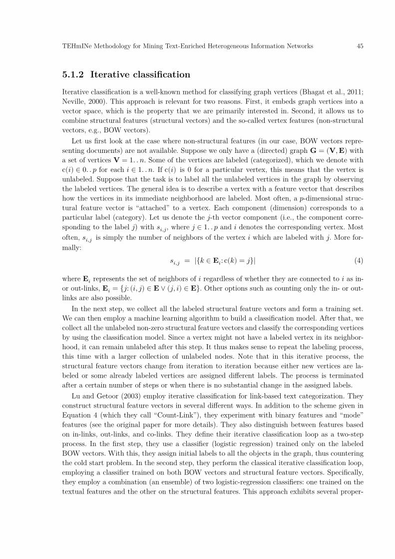
TEHmINe Methodology for Mining Text-Enriched Heterogeneous Information Networks 45
5.1.2 Iterative classification
Iterative classification is a well-known method for classifying graph vertices (Bhagat et al., 2011; Neville, 2000). This approach is relevant for two reasons. First, it embeds graph vertices into a vector space, which is the property that we are primarily interested in. Second, it allows us to combine structural features (structural vectors) and the so-called vertex features (non-structural vectors, e.g., BOW vectors).
Let us first look at the case where non-structural features (in our case, BOW vectors repre-senting documents) are not available. Suppose we only have a (directed) graph 𝐆𝐆 = (𝐕𝐕,𝐄𝐄) with a set of vertices 𝐕𝐕 = 1. . 𝑛𝑛. Some of the vertices are labeled (categorized), which we denote with c(𝑖𝑖) ∈ 0. . 𝑝𝑝 for each 𝑖𝑖 ∈ 1. . 𝑛𝑛. If c(𝑖𝑖) is 0 for a particular vertex, this means that the vertex is unlabeled. Suppose that the task is to label all the unlabeled vertices in the graph by observing the labeled vertices. The general idea is to describe a vertex with a feature vector that describes how the vertices in its immediate neighborhood are labeled. Most often, a 𝑝𝑝-dimensional struc-tural feature vector is “attached” to a vertex. Each component (dimension) corresponds to a particular label (category). Let us denote the 𝑗𝑗-th vector component (i.e., the component corre-sponding to the label 𝑗𝑗) with 𝑠𝑠𝑖𝑖,𝑗𝑗, where 𝑗𝑗 ∈ 1. . 𝑝𝑝 and 𝑖𝑖 denotes the corresponding vertex. Most often, 𝑠𝑠𝑖𝑖,𝑗𝑗 is simply the number of neighbors of the vertex 𝑖𝑖 which are labeled with 𝑗𝑗. More for-mally:
𝑠𝑠𝑖𝑖,𝑗𝑗 = |{𝑘𝑘 ∈ 𝐄𝐄𝑖𝑖: c(𝑘𝑘) = 𝑗𝑗}| (4)
where 𝐄𝐄𝑖𝑖 represents the set of neighbors of 𝑖𝑖 regardless of whether they are connected to 𝑖𝑖 as in- or out-links, 𝐄𝐄𝑖𝑖 = {𝑗𝑗: (𝑖𝑖, 𝑗𝑗) ∈ 𝐄𝐄 ∨ (𝑗𝑗, 𝑖𝑖) ∈ 𝐄𝐄}. Other options such as counting only the in- or out-links are also possible.
In the next step, we collect all the labeled structural feature vectors and form a training set. We can then employ a machine learning algorithm to build a classification model. After that, we collect all the unlabeled non-zero structural feature vectors and classify the corresponding vertices by using the classification model. Since a vertex might not have a labeled vertex in its neighbor-hood, it can remain unlabeled after this step. It thus makes sense to repeat the labeling process, this time with a larger collection of unlabeled nodes. Note that in this iterative process, the structural feature vectors change from iteration to iteration because either new vertices are la-beled or some already labeled vertices are assigned different labels. The process is terminated after a certain number of steps or when there is no substantial change in the assigned labels.
Lu and Getoor (2003) employ iterative classification for link-based text categorization. They construct structural feature vectors in several different ways. In addition to the scheme given in Equation 4 (which they call “Count-Link”), they experiment with binary features and “mode” features (see the original paper for more details). They also distinguish between features based on in-links, out-links, and co-links. They define their iterative classification loop as a two-step process. In the first step, they use a classifier (logistic regression) trained only on the labeled BOW vectors. With this, they assign initial labels to all the objects in the graph, thus countering the cold start problem. In the second step, they perform the classical iterative classification loop, employing a classifier trained on both BOW vectors and structural feature vectors. Specifically, they employ a combination (an ensemble) of two logistic-regression classifiers: one trained on the textual features and the other on the structural features. This approach exhibits several proper-

46 TEHmINe Methodology for Mining Text-Enriched Heterogeneous Information Networks
ties related to our methodology: (i) it combines textual and structural data, (ii) it embeds struc-tural data into a vector space, and (iii) it performs a data fusion step for combining the two different types of data.
5.1.3 Diffusion kernels
Kernels are structures that implicitly project a set of objects into a high-dimensional vector space by providing, for each pair of objects, the value of the dot product in that vector space. The algorithms that perform knowledge discovery with kernels (called the kernel methods), do not rely on explicit descriptions (i.e., vectors) of objects but rather perform all the necessary compu-tation by using the dot product values provided in a kernel matrix.
Kernels often model a notion of similarity between objects and therefore knowledge discovery is performed in an implicit vector space where the dot product corresponds to a similarity meas-ure between the vector representations of the objects. Diffusion kernels (Gärtner, 2003; Kondor and Lafferty, 2002) also fall into this category and model similarities between vertices in a weighted graph.
For our purpose, diffusion kernels are interesting because every kernel matrix 𝐊𝐊, by definition, can be represented as 𝐊𝐊 = 𝐕𝐕𝐕𝐕T, where the rows of 𝐕𝐕 can be viewed as vectors, effectively em-bedding the objects into a vector space in which the dot product between these objects behaves according to the definition in the kernel matrix.
Diffusion kernels are best explained with an analogy of diffusing randomly generated values across the network. Let us consider attaching a random variable 𝑍𝑍𝑖𝑖 to each vertex 𝑖𝑖 in an undi-rected weighted graph 𝐆𝐆 = (𝐕𝐕,𝐄𝐄,w). Now let each variable send some of its value (fraction 𝛼𝛼) to each of the immediate neighbors at discrete time steps 𝑡𝑡 = 1,2,3,… according to the following formula:
𝑍𝑍𝑖𝑖(𝑡𝑡 + 1) = 𝑍𝑍𝑖𝑖(𝑡𝑡) + 𝛼𝛼∑ 𝑤𝑤𝑖𝑖,𝑗𝑗(𝑍𝑍𝑗𝑗(𝑡𝑡) − 𝑍𝑍𝑖𝑖(𝑡𝑡))𝑗𝑗:∃{𝑖𝑖,𝑗𝑗}∈𝐄𝐄 (5)
where 𝑤𝑤𝑖𝑖,𝑗𝑗 denotes the weight (nonnegative) of the edge between 𝑖𝑖 and 𝑗𝑗. It turns out that the covariance matrix of such random field is a kernel reflecting similarities between vertices: the more two vertices 𝑖𝑖 and 𝑗𝑗 are interconnected in a graph, the more of 𝑍𝑍𝑖𝑖 is transitioned to 𝑍𝑍𝑗𝑗 and vice versa. Covariance between 𝑖𝑖 and 𝑗𝑗 is consequently increased. It is also possible to draw sim-ilarities between diffusion kernels and random walks (see Kondor and Lafferty, 2002).
A diffusion kernel is defined as follows:
𝐊𝐊𝐆𝐆 = lim𝑛𝑛→∞
∑ (𝛽𝛽𝐇𝐇)𝑡𝑡
𝑖𝑖!𝑛𝑛𝑖𝑖=0 (?)
𝐇𝐇 = −𝐋𝐋 = �ℎ1,1 … ℎ1,𝑛𝑛
⋮ ⋱ ⋮ℎ𝑛𝑛,1 … ℎ𝑛𝑛,𝑛𝑛
�, ℎ𝑖𝑖,𝑗𝑗 =⎩�⎨�⎧𝑤𝑤𝑖𝑖,𝑗𝑗 ∃{𝑖𝑖, 𝑗𝑗} ∈ 𝐄𝐄
− ∑ 𝑤𝑤𝑖𝑖,𝑘𝑘𝑘𝑘:∃{𝑖𝑖,𝑘𝑘}∈𝐄𝐄 𝑖𝑖 = 𝑗𝑗0 otherwise
(?)
where 𝑛𝑛 is the number of vertices in the graph, 𝐇𝐇 is the negative graph Laplacian −𝐋𝐋 (used as a generator), and 𝛽𝛽 is the diffusion parameter incorporating both 𝛼𝛼 and 𝑡𝑡 from Equation 5. A diffusion kernel can be relatively efficiently computed by first performing eigenvalue decomposi-tion of the negative Laplacian and thus obtaining 𝐇𝐇 = 𝐓𝐓𝐃𝐃𝐓𝐓T, and then computing the following (Gärtner, 2003):
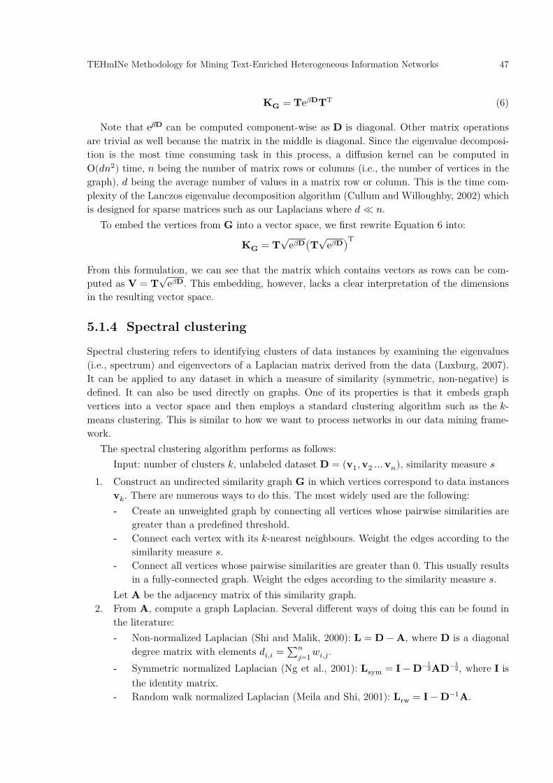
TEHmINe Methodology for Mining Text-Enriched Heterogeneous Information Networks 47
𝐊𝐊𝐆𝐆 = 𝐓𝐓e𝛽𝛽𝐃𝐃𝐓𝐓T (6)
Note that eβ𝐃𝐃 can be computed component-wise as 𝐃𝐃 is diagonal. Other matrix operations are trivial as well because the matrix in the middle is diagonal. Since the eigenvalue decomposi-tion is the most time consuming task in this process, a diffusion kernel can be computed in O(𝑑𝑑𝑛𝑛2) time, 𝑛𝑛 being the number of matrix rows or columns (i.e., the number of vertices in the graph), 𝑑𝑑 being the average number of values in a matrix row or column. This is the time com-plexity of the Lanczos eigenvalue decomposition algorithm (Cullum and Willoughby, 2002) which is designed for sparse matrices such as our Laplacians where 𝑑𝑑 ≪ 𝑛𝑛.
To embed the vertices from 𝐆𝐆 into a vector space, we first rewrite Equation 6 into:
𝐊𝐊𝐆𝐆 = 𝐓𝐓√
e𝛽𝛽𝐃𝐃�𝐓𝐓√
e𝛽𝛽𝐃𝐃�T (?)
From this formulation, we can see that the matrix which contains vectors as rows can be com-puted as 𝐕𝐕 = 𝐓𝐓
√e𝛽𝛽𝐃𝐃. This embedding, however, lacks a clear interpretation of the dimensions
in the resulting vector space.
5.1.4 Spectral clustering
Spectral clustering refers to identifying clusters of data instances by examining the eigenvalues (i.e., spectrum) and eigenvectors of a Laplacian matrix derived from the data (Luxburg, 2007). It can be applied to any dataset in which a measure of similarity (symmetric, non-negative) is defined. It can also be used directly on graphs. One of its properties is that it embeds graph vertices into a vector space and then employs a standard clustering algorithm such as the 𝑘𝑘-means clustering. This is similar to how we want to process networks in our data mining frame-work.
The spectral clustering algorithm performs as follows: Input: number of clusters 𝑘𝑘, unlabeled dataset 𝐃𝐃 = (𝐯𝐯1, 𝐯𝐯2 …𝐯𝐯𝑛𝑛), similarity measure 𝑠𝑠
1. Construct an undirected similarity graph 𝐆𝐆 in which vertices correspond to data instances 𝐯𝐯𝑘𝑘. There are numerous ways to do this. The most widely used are the following: - Create an unweighted graph by connecting all vertices whose pairwise similarities are
greater than a predefined threshold. - Connect each vertex with its 𝑘𝑘-nearest neighbours. Weight the edges according to the
similarity measure 𝑠𝑠. - Connect all vertices whose pairwise similarities are greater than 0. This usually results
in a fully-connected graph. Weight the edges according to the similarity measure 𝑠𝑠. Let 𝐀𝐀 be the adjacency matrix of this similarity graph.
2. From 𝐀𝐀, compute a graph Laplacian. Several different ways of doing this can be found in the literature: - Non-normalized Laplacian (Shi and Malik, 2000): 𝐋𝐋 = 𝐃𝐃 − 𝐀𝐀, where 𝐃𝐃 is a diagonal
degree matrix with elements 𝑑𝑑𝑖𝑖,𝑖𝑖 = ∑ 𝑤𝑤𝑖𝑖,𝑗𝑗𝑛𝑛𝑗𝑗=1 .
- Symmetric normalized Laplacian (Ng et al., 2001): 𝐋𝐋sym = 𝐈𝐈 − 𝐃𝐃−12𝐀𝐀𝐃𝐃−1
2, where 𝐈𝐈 is the identity matrix.
- Random walk normalized Laplacian (Meila and Shi, 2001): 𝐋𝐋rw = 𝐈𝐈 − 𝐃𝐃−1𝐀𝐀.
48 TEHmINe Methodology for Mining Text-Enriched Heterogeneous Information Networks
3. Compute the first 𝑘𝑘 eigenvectors 𝐮𝐮1, 𝐮𝐮2,… , 𝐮𝐮𝑘𝑘. By “the first eigenvectors”, we refer to the eigenvectors corresponding to the smallest eigenvalues. In (Shi and Malik, 2000), the first 𝑘𝑘 generalized eigenvectors are computed instead by solving the generalized eigenvalue prob-lem 𝐋𝐋𝐮𝐮 = 𝜆𝜆𝐃𝐃𝐮𝐮. This makes it equivalent to computing 𝐋𝐋rw and solving the standard ei-genvalue problem.
4. Let 𝐔𝐔 be the matrix containing the eigenvectors as columns and let 𝐱𝐱𝑘𝑘 be the vector cor-responding to the 𝑘𝑘-th row of 𝐔𝐔. In (Ng et al., 2001), the authors normalize the vectors 𝐱𝐱𝑘𝑘 so that their Euclidean norm is 1.
5. Cluster the vectors 𝐱𝐱𝑘𝑘 into 𝑘𝑘 clusters. Usually, the 𝑘𝑘-means clustering algorithm is used for this purpose. Note that it is also possible to replace 𝑘𝑘-means with some other clustering algorithm (e.g., hyperplane-based clustering; Lang, 2005). Either way, it has been shown that the Euclidean distance is a meaningful measure for determining clusters in the result-ing space (Nadler et al., 2005).
Spectral clustering can also be used directly on graphs by simply skipping the first step and starting by computing a graph Laplacian. Essentially, this algorithm embeds a graph into a 𝑘𝑘-dimensional Euclidean space (where 𝑘𝑘 is normally relatively small) in which clustering is per-formed to determine meaningful groups of vertices.
It can be shown that for a connected, non-bipartite graph 𝐆𝐆 = (𝐕𝐕,𝐄𝐄) and two disjoint sets of vertices 𝐀𝐀,𝐁𝐁 ⊂ 𝐕𝐕, the bisecting 𝐋𝐋rw-based spectral clustering looks for the cut that minimizes the probability that a random walker will transition from one set of vertices to another or vice versa (Meila and Shi, 2001).
5.1.5 PageRank and Personalized PageRank
PageRank is a measure of relative importance of a vertex in a directed weighted graph (Page et al., 1999). It is named after one of its inventors, Larry Page (Google), and was originally used to rank web pages in the Google search engine (which makes the name PageRank an amusing word play). A variant of the algorithm, called Personalized PageRank (PPR), can also be used for embedding networks into vector spaces (Page et al., 1999).
The classical PageRank algorithm takes as input a directed weighted graph and assigns an importance weight to each vertex in the graph. A highly weighted vertex is more important in the sense that many vertices (that are themselves also relatively highly weighted) point directly to it. The algorithm can be intuitively explained with the random walker paradigm as follows:
1. The random walker starts at an arbitrary vertex. 2. The random walker decides whether to move or not; it moves with the probability
P(move) = 𝑑𝑑, where 𝑑𝑑 is the so-called damping factor. 3. If it decides to move, it chooses one of the outgoing edges to move along. An edge is chosen
with the probability proportional to the edge weight (with respect to the weights of the other outgoing edges).
4. If it decides not to move, it is “teleported” to a randomly selected vertex. 5. The process is repeated from Step 2.
The weight assigned to a vertex is intuitively the relative number of times the random walker visits the vertex in an infinitely long walk. In other words, it is the probability that such random walker will be, at a random point in time, observed at a particular vertex.
TEHmINe Methodology for Mining Text-Enriched Heterogeneous Information Networks 49
A PageRank vector 𝐫𝐫 is more formally defined as follows:
𝐫𝐫 = (1 − 𝑑𝑑)𝐭𝐭 + 𝑑𝑑(𝐫𝐫𝐫𝐫) (7)
𝐭𝐭 = [ 1𝑁𝑁 , 1
𝑁𝑁 , … , 1𝑁𝑁] (?)
where 𝑑𝑑 ∈ [0,1] is the damping factor, 1 − 𝑑𝑑 is the teleport probability, 𝐭𝐭 is the teleport vector, and 𝐫𝐫 is the row-normalized adjacency matrix (i.e., right stochastic matrix). Vector 𝐭𝐭 contains the probabilities that the random walker will choose a particular vertex when teleporting. In the original formulation, these probabilities are all set to 1
𝑁𝑁, where 𝑁𝑁 is the number of vertices (i.e., choosing each vertex with equal probability).
A simple way to show that 𝐫𝐫 is in fact a stationary distribution over a modified adjacency matrix is to insert the teleport edges into the underlying graph. This also reveals that the above equation is not entirely correct if the graph contains vertices with no out-links (called dangling links in the original paper; we will call them dangling vertices instead). Suppose that we have a graph 𝐆𝐆 = (𝐕𝐕, 𝐄𝐄,w) in which every vertex has at least one outgoing edge (i.e., no dangling links). From 𝐆𝐆, we now construct a graph 𝐆𝐆′ which more explicitly models the behaviour of the random walker. We first normalize the weights of the outgoing edges at each vertex so that they sum up to 1:
∀𝑖𝑖: ∑ w(𝑖𝑖, 𝑗𝑗)𝑗𝑗:(𝑖𝑖,𝑗𝑗)∈𝐄𝐄 = 1 (8)
Then, we multiply these weights with 𝑑𝑑 (the probability of continuing the walk). Next, we add 𝑁𝑁 outgoing teleport edges to each vertex, each weighted with 1−𝑑𝑑
𝑁𝑁 , so that each other vertex can be directly reached through a teleport edge. This construction exactly corresponds to Equation 7. If we now consider the adjacency matrix 𝐀𝐀 (which is row-normalized), we can describe the PageRank vector 𝐫𝐫 as 𝐫𝐫 = 𝐫𝐫𝐀𝐀.
However, suppose that 𝐆𝐆 has at least one vertex with no outgoing edges (i.e., a dangling vertex) to which the condition given in Equation 8 clearly cannot be applied. If we apply the previously discussed graph reconstruction process, the weights of the outgoing teleport edges at a dangling vertex sum up to 1 − 𝑑𝑑. In order to get a stochastic adjacency matrix (with normalized rows), we thus need to divide the weights of the teleport edges at dangling vertices with 1 − 𝑑𝑑. In other words, at a dangling vertex, the teleport edges should be weighted with 1
𝑁𝑁. This kind of construction, which does not entirely correspond to Equation 7, gives us the proper PageRank equation 𝐫𝐫 = 𝐫𝐫𝐀𝐀, where 𝐀𝐀 is a row-normalized stochastic matrix even if the graph contains dan-gling vertices. If 𝑑𝑑 is set to 1, 𝐫𝐫 = 𝐫𝐫𝐀𝐀 becomes 𝐫𝐫 = 𝐫𝐫𝐫𝐫 (see Equation 7). Since the stationary distribution does not always exist for an arbitrary graph, the convergence cannot be guaranteed. On the other hand, if we set 𝑑𝑑 to 0, we have the solution 𝐫𝐫 = 𝐭𝐭 which does not tell us anything about the general importance of vertices. However, if 𝑑𝑑 is greater than 0 and smaller than 1, we end up with a Markov chain in which every state is positive recurrent and for which a unique stationary distribution is guaranteed to exist (Online reference [2]). In this case, the PageRank vector 𝐫𝐫 is essentially the only eigenvector of 𝐀𝐀 (with the corresponding eigenvalue 𝜆𝜆 = 1). In practice, PageRank is often computed iteratively as follows:
1. Initialize PageRank vector: 𝐫𝐫 = [ 1𝑁𝑁 , 1
𝑁𝑁 , … , 1𝑁𝑁].
2. Set 𝐭𝐭 = [ 1𝑁𝑁 , 1
𝑁𝑁 , … , 1𝑁𝑁].
3. Compute 𝐫𝐫′ = (1 − 𝑑𝑑)𝐭𝐭 + 𝑑𝑑(𝐫𝐫𝐫𝐫).

50 TEHmINe Methodology for Mining Text-Enriched Heterogeneous Information Networks
4. Because of the dangling vertices (if any), the difference 𝑒𝑒 = 1 − ‖𝐫𝐫′‖1 can be greater than 0. In this case, we distribute it among all the vertices: 𝐫𝐫′′ = 𝐫𝐫′ + 𝑒𝑒𝐭𝐭. Otherwise 𝐫𝐫′′ = 𝐫𝐫′.
5. Compute 𝛿𝛿 = ‖𝐫𝐫′′ − 𝐫𝐫‖1. If 𝛿𝛿 is greater than some (predefined) small positive 𝜀𝜀, end the algorithm and return 𝒓𝒓′′.
6. Repeat from Step 3 (with 𝐫𝐫 ← 𝐫𝐫′′).
By modifying the teleport vector 𝐭𝐭, it is possible to redefine the teleporting strategy of the random walker. If the teleport probability in 𝐭𝐭 is not equally distributed, we call such ranking algorithm Personalized PageRank (PPR). The way PPR is normally used is that we define a set of 𝑚𝑚 source vertices 𝐒𝐒 ⊆ 𝐕𝐕, |𝐒𝐒| = 𝑚𝑚, and modify the teleport vector (and also the initial PPR vector 𝐫𝐫) so that it contains 1
𝑚𝑚 for every vertex 𝑖𝑖 ∈ 𝐒𝐒 and 0 for all other vertices. A special case of this kind of PPR is when we select only one vertex as the source, |𝐒𝐒| = 𝑚𝑚 = 1. In this case, the corresponding teleport vector component is 1 and all the others are 0. In general, we could say that PPR ranks vertices in a graph with respect to a set of source vertices. Even more accurately, it ranks vertices with respect to the vertex probability distribution in 𝐭𝐭. PPR can also be used for embedding networks into vector spaces. We discuss this aspect of PPR more thor-oughly later on in Section 5.2.
5.1.6 SimRank
As the last algorithm in this section, we discuss SimRank (Jeh and Widom, 2002), a measure of similarity between vertices based on their structural contexts. In contrast to the other discussed algorithms, SimRank does not embed vertices into a vector space. The reason for presenting it here is that it introduces the notion of expected meeting distance, a concept similar to the one that we use to provide intuition for the development of a similarity measure in our data mining framework (see Section 5.2.2).
SimRank is also interesting because it does not assume that two directly connected vertices are similar to each other. It only assumes that a vertex is similar to itself and that two vertices are similar if vertices that are also similar to each other link to them.
The SimRank measure between two vertices a and b in a graph, s(a, b), is defined recursively as follows:
s(𝑎𝑎, 𝑎𝑎) = 1 (?)
s(𝑎𝑎, 𝑏𝑏) = 𝐶𝐶|𝐈𝐈𝑎𝑎||𝐈𝐈𝑏𝑏| ∑ ∑ s(𝑖𝑖, 𝑗𝑗)𝑗𝑗∈𝐈𝐈𝑏𝑏𝑖𝑖∈𝐈𝐈𝑎𝑎
(?)
In this equation, 𝐈𝐈𝑎𝑎 and 𝐈𝐈𝑏𝑏 denote the set of vertices directly linked to 𝑎𝑎 and the set of vertices directly linked to 𝑏𝑏, respectively. More formally, for any vertex 𝑖𝑖, 𝐈𝐈𝑖𝑖 = {𝑗𝑗: (𝑗𝑗, 𝑖𝑖) ∈ 𝐄𝐄}. Note that if either |𝐈𝐈𝑎𝑎| or |𝐈𝐈𝑏𝑏| is 0, the similarity score is defined to be 0. 𝐶𝐶 plays the role of a damping factor.
SimRank over 𝐆𝐆 can also be interpreted in the sense of random walks. Let us define the expected distance between vertices 𝑖𝑖 and 𝑗𝑗 in 𝐆𝐆 as:
d(𝑖𝑖, 𝑗𝑗) = ∑ P(𝐭𝐭)l(𝐭𝐭)𝐭𝐭:𝑖𝑖→𝑗𝑗 (?)
where 𝐭𝐭 is a tour from 𝑖𝑖 to 𝑗𝑗, P(𝐭𝐭) is a probability that the random walker will make the tour 𝐭𝐭, and l(𝐭𝐭) is the length (in the number of edges) of the tour 𝐭𝐭. The expected distance d(𝑖𝑖, 𝑗𝑗) is in

TEHmINe Methodology for Mining Text-Enriched Heterogeneous Information Networks 51
fact the expected number of steps that the random walker needs to take to get from 𝑖𝑖 to 𝑗𝑗. If the tours have cycles, the above equation is a convergent infinite sum.
Let us now derive, from 𝐆𝐆, a graph of vertex pairs 𝐆𝐆2:
𝐆𝐆2 = (𝐕𝐕2,𝐄𝐄2) (?)
𝐕𝐕2 = {(𝑖𝑖, 𝑗𝑗): 𝑖𝑖, 𝑗𝑗 ∈ 𝐕𝐕} (?)
𝐄𝐄2 = {⟨(𝑖𝑖, 𝑗𝑗), (𝑘𝑘, 𝑙𝑙)⟩: (𝑖𝑖, 𝑗𝑗), (𝑘𝑘, 𝑙𝑙) ∈ 𝐕𝐕2 ∧ (𝑖𝑖, 𝑘𝑘), (𝑗𝑗, 𝑙𝑙) ∈ 𝐄𝐄} (?)
A vertex pair (𝑖𝑖, 𝑗𝑗) points to a pair (𝑘𝑘, 𝑙𝑙) in 𝐆𝐆2 if, in 𝐆𝐆, 𝑖𝑖 points to 𝑘𝑘 and 𝑗𝑗 points to 𝑙𝑙. In this derived graph, a random walker starting in (𝑖𝑖, 𝑗𝑗) and ending in (𝑘𝑘, 𝑘𝑘) represents two random walkers in 𝐆𝐆, one starting from 𝑖𝑖, the other from 𝑗𝑗, which meet each other in vertex 𝑘𝑘. This allows us to elegantly model the concept of the expected meeting distance:
m(𝑖𝑖, 𝑗𝑗) = ∑ P(𝐭𝐭)l(𝐭𝐭)𝐭𝐭:(𝑖𝑖,𝑗𝑗)→(𝑘𝑘,𝑘𝑘) (9)
m(𝑖𝑖, 𝑗𝑗) gives us the expected number of steps that each of the two random walkers in 𝐆𝐆, one starting from 𝑖𝑖, the other from 𝑗𝑗, need to take before they meet. For various reasons (see the original paper for details), it is more convenient to turn this equation into a similarity measure by mapping the range of l(𝐭𝐭) , i.e., [0,∞) , onto (0,1] by substituting l(𝐭𝐭) with 𝑐𝑐l(𝐭𝐭) , where 𝑐𝑐 ∈(0,1). This maps paths of length 0 to 1 and extremely long paths to a value close to 0. Equation 9 thus becomes:
s′(𝑖𝑖, 𝑗𝑗) = ∑ P(𝐭𝐭)𝑐𝑐l(𝐭𝐭)𝐭𝐭:(𝑖𝑖,𝑗𝑗)→(𝑘𝑘,𝑘𝑘) (?)
It can be shown that:
s′(𝑎𝑎, 𝑏𝑏) = 𝑐𝑐|𝐎𝐎𝑎𝑎||𝐎𝐎𝑏𝑏| ∑ ∑ s′(𝑖𝑖, 𝑗𝑗)𝑗𝑗∈𝐎𝐎𝑏𝑏𝑖𝑖∈𝐎𝐎𝑎𝑎
(?)
In this equation, 𝐎𝐎𝑎𝑎 and 𝐎𝐎𝑏𝑏 denote the set of vertices directly linked from 𝑎𝑎 and the set of ver-tices directly linked from 𝑏𝑏, respectively. In other words, the similarity score based on the ex-pected meeting distance is in fact SimRank with a damping factor 𝐶𝐶 = 𝑐𝑐 and focusing on out-links rather than in-links. If the two random walkers followed in-links rather than out-links in their walks, the above equation would turn into the SimRank equation. The two random walkers would meet in nodes that represent sources of rank. SimRank is therefore a similarity measure closely related to the expected meeting distance of two random walkers in a graph.
5.2 Embedding networks into BOW-like spaces
We already provided the rationale for extending an existing text mining framework with network analysis capabilities in Chapter 3. As evident from the methodology overview presented in Figure 3.3, the main missing piece of the methodology workflow is the component for embedding heter-ogeneous information networks into BOW-like vector spaces that can be combined with a BOW space to form a common vector space in which knowledge discovery can be performed. We develop this missing piece in this section.
52 TEHmINe Methodology for Mining Text-Enriched Heterogeneous Information Networks
5.2.1 Argumentation for choosing Personalized PageRank
From the approaches, presented in Section 5.1, we have selected Personalized PageRank (PPR) for embedding networks into vector spaces. Our choice was mainly guided by the idea of defining a common space in which both texts and vertices can be represented. Furthermore, one of the requirements states that the same analytical tools need to be able to handle each type of data separately and both types of data in combination (the “uniformity” requirement, see Section 3.2). Since the functional basis for TEHmINe is LATINO, a text-mining toolkit based on the BOW vector representation of texts, the resulting structural vectors are required to demonstrate certain properties of BOW vectors.
In practice, when working with BOW vectors, we can observe the following (relatively obvious) properties:
1. BOW vectors can be constructed regardless of the type of the given data mining task (e.g., it can be either a classification or a clustering task). This is the most important property because our goal is to devise a general-purpose methodology.
2. BOW vectors are high-dimensional and sparse. In addition, by removing components with low weights (i.e., cutting off tails), it is possible to make the analyses more efficient (lower memory consumption, faster similarity computations) without compromising the quality of the results.
3. Cosine similarity is the similarity metric of choice when working with BOW vectors. Intu-itively, it compares two documents according to content, disregarding their lengths.
4. The components of a BOW vector (and thus the dimensions of the corresponding BOW space) have a clear interpretation. They represent terms from the source text corpus.
Let us now review the approaches presented in Section 5.1 with respect to these properties. The iterative classification algorithm (Section 5.1.2) is not suitable for our needs because it requires labeled data in order to construct structural feature vectors. This limits the approach to super-vised learning, which immediately rules it out for using it in a general-purpose framework. In addition, the constructed structural feature vectors are normally low-dimensional (the number of dimensions is the number of different labels in the training set). They, however, do have a clear interpretation and can intuitively be compared with the cosine similarity measure.
Diffusion kernels (Section 5.1.3) clearly violate the fourth property as the corresponding vec-tor-space representation does not come with a clear interpretation of the dimensions. By defini-tion, the dot product represents a well-grounded measure of similarity between two “diffusion vectors”. It is however unclear whether applying the cosine similarity makes sense (note that the diffusion vectors are not normalized and thus using cosine similarity is not equivalent to using dot product). On the other hand, they can be constructed regardless of the type of the data mining task at hand, which is a desirable property.
Spectral clustering (Section 5.1.4) normally constructs low-dimensional vectors, where the number of dimensions is equal to the number of target clusters. This implies that the process cannot be used in a general-purpose setting. Furthermore, the vectors are constructed from ei-genvectors of a Laplacian matrix, which makes the process relatively complex. From this per-spective, it is not clear what the dimensions of the resulting space intuitively mean. Finally, while it was shown that the Euclidean distance discriminates well between the resulting clusters (Nadler et al., 2005), there is no guarantee that the cosine similarity measure performs equally well.

TEHmINe Methodology for Mining Text-Enriched Heterogeneous Information Networks 53
Finally, Personalized PageRank (PPR), when run from a single vertex, produces a structural vector for that vertex (see Section 5.1.5). It can be shown that PPR vectors demonstrate many properties of BOW vectors. First of all, they can be constructed regardless of the type of the subsequent data mining task. They are relatively high-dimensional (the number of dimensions equals the number of vertices in the graph) and can be usually made sparse by removing low weights (analogous to cutting off tails of BOW vectors). Furthermore, they work well with both the dot product and the cosine similarity. For both these two similarity measures, it is also possible to provide intuitive interpretations (see Section 5.2.2). Finally, the components of a PPR vector do have a clear interpretation (they represent the vertices in the graph).
From this discussion, we can conclude that, among the discussed approaches, PPR is the most suitable choice for embedding networks into BOW-like spaces. We discuss an intuitive interpre-tation of using cosine similarity with PPR vectors in the following subsection.
5.2.2 Similarity measure in the PPR vector space
To embed a network into a vector space, we employ Personalized Page Rank (PPR), discussed in Section 5.1.5. The term “personalized” refers to using a predefined set of vertices as the source of rank; in our case, PPR is run from a single source vertex in a directed weighted graph 𝐆𝐆 =(𝐕𝐕,𝐄𝐄,𝑤𝑤). This vertex represents the object for which we want to compute the structural vector.
The process is equivalent to a random walk that starts at a particular vertex. At each vertex, the random walker decides whether to teleport back to the source vertex (this is done with the probability 1 − 𝑑𝑑 where 𝑑𝑑 is the so-called damping factor) or to continue its walk along one of the edges. The probability of choosing a certain edge is proportional to this edge’s weight with respect to the weights of the other edges attached to the vertex. In effect, for a selected source vertex 𝑖𝑖 in a graph, PPR computes a vector with components 𝑟𝑟𝑖𝑖,𝑗𝑗, where 𝑗𝑗 is a vertex in the graph and 𝑟𝑟𝑖𝑖,𝑗𝑗 is the probability that the random walker starting from vertex 𝑖𝑖 will be observed at vertex 𝑗𝑗 at an arbitrary point in time.
This process projects a node 𝑖𝑖 into a PPR vector space or, in other words, represents the node 𝑖𝑖 with a PPR vector. We will now show that the dot product of two such vectors represents a similarity measure with a clear intuitive interpretation. Let us first define two single-source PPR vectors (one starting from 𝑖𝑖 and the other from 𝑗𝑗):
𝐱𝐱𝑖𝑖 = �𝑟𝑟𝑖𝑖,1, 𝑟𝑟𝑖𝑖,2, … , 𝑟𝑟𝑖𝑖,𝑚𝑚�, 𝐱𝐱𝑗𝑗 = (𝑟𝑟𝑗𝑗,1, 𝑟𝑟𝑗𝑗,2,… , 𝑟𝑟𝑗𝑗,𝑚𝑚) (?)
The dot product of the two vectors is defined as follows:
𝐱𝐱𝑖𝑖 ⋅ 𝐱𝐱𝑗𝑗 = 𝑟𝑟𝑖𝑖,1𝑟𝑟𝑗𝑗,1 + 𝑟𝑟𝑖𝑖,2𝑟𝑟𝑗𝑗,2 + ⋯+ 𝑟𝑟𝑖𝑖,𝑚𝑚𝑟𝑟𝑗𝑗,𝑚𝑚 (10)
Because observing one random walker at a particular vertex is independent from observing the other at that same vertex, we can interpret a product 𝑟𝑟𝑖𝑖,𝑘𝑘𝑟𝑟𝑗𝑗,𝑘𝑘 as the probability that the random walker starting from vertex 𝑖𝑖 will be observed at vertex 𝑘𝑘 and at the same time, the random walker starting from 𝑗𝑗 will be observed at 𝑘𝑘 at an arbitrary point in time. In other words, this product denotes the probability that the two random walkers meet at vertex 𝑘𝑘 at an arbitrary point in time. Furthermore, because the separate meeting events are mutually exclusive (i.e., disjoint), we can interpret the dot product given in Equation 10 as “the probability that the two random walkers, one starting from 𝑖𝑖 and the other from 𝑗𝑗, meet at vertex 1 or at vertex 2 or ... or at vertex 𝑚𝑚 at an arbitrary point in time”. In other words, the presented dot product denotes

54 TEHmINe Methodology for Mining Text-Enriched Heterogeneous Information Networks
the probability that the two random walkers meet (at an arbitrary vertex) at an arbitrary point in time. This principle is illustrated in Figure 5.1.
Although this gives a very nice justification for using dot product as a measure of similarity, it does not fulfill our requirement of having an intuitive justification for using the cosine similarity measure. We now offer a reinterpretation of similarity between vertices in which we perceive random walks as text documents. This reinterpretation also makes an important connection be-tween bags-of-words and Personalized PageRank thus placing it nicely into our BOW-based framework.
Let us suppose that each node is assigned a random word and that a single random walker, staring his walk from a particular vertex, is “writing down” the words that it encounters along the way. In other words, we can view the graph as a simple stochastic language model (this principle is illustrated in Figure 5.2). This view works if we assume that the clusters in the graph (i.e., highly interconnected groups of vertices) correspond to topics. If two random walkers start from within the same cluster, they tend to stay within the cluster (because the connectedness within the cluster is greater than that between the clusters). For this reason, the resulting two random documents will mostly contain words from the same cluster or, in other words, they will discuss the same topic. From the “random writer” perspective, a PPR vector is in fact the 𝑙𝑙1-normalized (i.e., vector components sum up to 1) term-frequency (TF) BOW vector representa-tion of the corresponding (infinite) random text document.
This intuitively justifies the use of cosine similarity when comparing two PPR vectors. It also relates PPR vectors to bags-of-words and thus nicely fits PPR into our existing text mining framework.
5.2.3 Decomposing heterogeneous networks into homogeneous graphs
As already discussed in Section 5.1.5, PPR is applicable to directed weighted graphs. Heteroge-neous information networks (HINs) are indeed directed and weighted (see Section 5.1.1) but they
Figure 5.1: Dot product in a PPR space: the meeting probability. The vectors x1 and x7 contain PPR weights (visit probabilities) for the random walks starting from the nodes 1 and 7, respec-tively. The probability that the two walkers meet at an arbitrary node is 7.74%.
x1 = (0.30, 0.19, 0.23, 0.11, 0.04, 0.06, 0.03, 0.04)
7
8
43
5
62
1
x7 = (0.03, 0.03, 0.06, 0.18, 0.09, 0.19, 0.27, 0.15)x7·x7 = 0.0774

TEHmINe Methodology for Mining Text-Enriched Heterogeneous Information Networks 55
also come with vertex- and edge-type information. This information is discarded if we feed a HIN to the PPR algorithm. We have therefore decided to decompose a HIN into a set of homogeneous context graphs with the following properties:
1. A context graph contains only one type of vertices and one type of edges. 2. The relation in a context graph models an aspect of similarity. 3. The relation in a context graph is implicitly reflexive. This means that every vertex is
related to itself. With respect to the first property, this intuitively makes sense as it states that every object is similar to itself. “Implicitly” here means that we do not need to explic-itly model this property by attaching a loop to each vertex.
4. The relation in a context graph is implicitly transitive. This means that if 𝑖𝑖 is related to 𝑗𝑗 and 𝑗𝑗 is related to 𝑘𝑘, then 𝑖𝑖 is also related to 𝑘𝑘. “Implicitly” here means that we do not need to explicitly model all the relations in the transitive closure.
5. The relation in a context graph is symmetric. This means that if vertex 𝑖𝑖 is related to vertex 𝑗𝑗, vertex 𝑗𝑗 is also related to vertex 𝑖𝑖. With respect to the second property, this intuitively makes sense as it states that if 𝑖𝑖 is similar to 𝑗𝑗, then 𝑗𝑗 is also similar to 𝑖𝑖. Effec-tively, this means that the context graph is a symmetric directed graph.
To argue for these requirements, let us again resort to the random-writer interpretation of PPR. The random writer starting from 𝑖𝑖 eventually visits all the vertices directly or indirectly reachable from 𝑖𝑖. This means that it writes down all the words assigned to these vertices but with different relative frequencies. Suppose that 𝑘𝑘 is a vertex reachable from 𝑖𝑖. If started from 𝑘𝑘, the random writer will undoubtedly write down the word attached to 𝑘𝑘. This means that both these two documents (one started from 𝑖𝑖 and the other from 𝑘𝑘) will contain the word attached to 𝑘𝑘. This will make the two vertices similar at least to some extent. In general, if 𝑘𝑘 is reachable from 𝑗𝑗, then 𝑗𝑗 will be similar to 𝑘𝑘 at least to some extent (transitivity). Furthermore, the cosine similarity of a vertex with itself will always be 1 (reflexivity). Finally, cosine similarity is a sym-metric similarity measure, which means that cossim(𝑎𝑎, 𝑏𝑏) = cossim(𝑏𝑏, 𝑎𝑎). Therefore, the use of
Figure 5.2: Cosine similarity in a PPR space: the random writer analogy. The vector x7 contains PPR weights (visit probabilities) for the random walk starting from the node to which the word “word7” is assigned. If we imagine that the random walker is “writing down” the words that it encounters along the way, then x7 can be seen as the l1-normalized term-frequency bag-of-words representation of the random document created by this random walker (hence the term “random writer”).
“word7 word6 word4 word3 ...”
word7
word8
word4word3
word5
word6word2
word1
x7 = (0.03, 0.03, 0.06, 0.18, 0.09, 0.19, 0.27, 0.15)
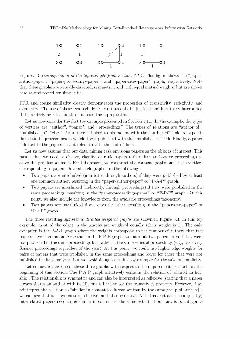
56 TEHmINe Methodology for Mining Text-Enriched Heterogeneous Information Networks
PPR and cosine similarity clearly demonstrates the properties of transitivity, reflexivity, and symmetry. The use of these two techniques can thus only be justified and intuitively interpreted if the underlying relation also possesses these properties.
Let us now consider the first toy example presented in Section 3.1.1. In the example, the types of vertices are “author”, “paper”, and “proceedings”. The types of relations are “author of”, “published in”, “cites”. An author is linked to his papers with the “author of” link. A paper is linked to the proceedings in which it was published with the “published in” link. Finally, a paper is linked to the papers that it refers to with the “cites” link.
Let us now assume that our data mining task envisions papers as the objects of interest. This means that we need to cluster, classify, or rank papers rather than authors or proceedings to solve the problem at hand. For this reason, we construct the context graphs out of the vertices corresponding to papers. Several such graphs are the following:
• Two papers are interlinked (indirectly, through authors) if they were published by at least one common author, resulting in the “paper-author-paper” or “P-A-P” graph.
• Two papers are interlinked (indirectly, through proceedings) if they were published in the same proceedings, resulting in the “paper-proceedings-paper” or “P-P-P” graph. At this point, we also include the knowledge from the available proceedings taxonomy.
• Two papers are interlinked if one cites the other, resulting in the “paper-cites-paper” or “P-c-P” graph.
The three resulting symmetric directed weighted graphs are shown in Figure 5.3. In this toy example, most of the edges in the graphs are weighted equally (their weight is 1). The only exception is the P-A-P graph where the weights correspond to the number of authors that two papers have in common. Note that in the P-P-P graph, we interlink two papers even if they were not published in the same proceedings but rather in the same series of proceedings (e.g., Discovery Science proceedings regardless of the year). At this point, we could use higher edge weights for pairs of papers that were published in the same proceedings and lower for those that were not published in the same year, but we avoid doing so in this toy example for the sake of simplicity.
Let us now review one of these three graphs with respect to the requirements set forth at the beginning of this section. The P-A-P graph intuitively contains the relation of “shared author-ship”. The relationship is symmetric and can also be interpreted as reflexive (stating that a paper always shares an author with itself), but is hard to see the transitivity property. However, if we reinterpret the relation as “similar in content [as it was written by the same group of authors]”, we can see that it is symmetric, reflexive, and also transitive. Note that not all the (implicitly) interrelated papers need to be similar in content to the same extent. If our task is to categorize
Figure 5.3: Decomposition of the toy example from Section 3.1.1. This figure shows the “paper-author-paper”, “paper-proceedings-paper”, and “paper-cites-paper” graph, respectively. Note that these graphs are actually directed, symmetric, and with equal mutual weights, but are shown here as undirected for simplicity.
12
1
3
2
4
111
3
2
41
1
3
1
1
2
4

TEHmINe Methodology for Mining Text-Enriched Heterogeneous Information Networks 57
or cluster papers according to their content, this relation indeed represents a notion of similarity. We can draw similar conclusions for the other two derived graphs.
Note that while the relation in a derived graph is transitive and reflexive only by interpretation (we do not model it explicitly as such), it needs to explicitly model the symmetry property. This means that for every edge there exists its reversed counterpart with the same weight. Such graph can also be interpreted as an undirected graph but strictly speaking, it is a symmetric directed graph. Looking again at our toy example, we can see that the first two derived graphs, the P-A-P graph and the P-P-P graph, are symmetric by design. The P-c-P graph, however, requires us to perform another step in the decomposition process and explicitly complement each edge with its reverse counterpart. In the event of already having a mutual edge between two vertices in such a graph (e.g., two papers mutually citing each other), we sum the two weights—let us denote this sum with 𝑤𝑤—and replace the two existing edges with two new edges, each of them weighted with 𝑤𝑤, one being the reversed counterpart of the other.
5.2.4 Fusing context vectors with BOW vectors
In Section 5.2.3, we argued for the decomposition of a heterogeneous information network (HIN) into a set of homogeneous graphs. In short, this makes it compatible with PPR, the algorithm of our choice for embedding networks into vector spaces (see Section 5.2). This decomposition ef-fectively produces a set of structural vectors for each vertex (one structural vector for each graph). Since our workflow (see Section 3.3) already envisions a data fusion component that joins textual and structural data, we can handle different network contexts (i.e., different homogeneous graphs) in the same data fusion framework to produce in the end one single vector (containing textual and heterogeneous structural information) for each object (vertex).
In this section, we present a simple and pragmatic data fusion model that we use as a building block in the proposed methodology. From a high-level perspective, we propose to concatenate the vectors (i.e., attaching one after the other) and apply a feature weighting (i.e., component weighting) scheme to account for the different types of data. The approach is illustrated in Figure 5.4.
To explain the theoretical background, we first establish a relationship between vectors and linear kernels. Suppose that, for a given object 𝑖𝑖, the concatenated vector is obtained by “gluing together” 𝑚𝑚 vectors (corresponding to the different modalities of data, e.g., one BOW vector and 𝑚𝑚 − 1 structural PPR vectors). For a given set of 𝑛𝑛 objects, let us denote the 𝑚𝑚 sets of feature vectors by 𝐕𝐕1,… , 𝐕𝐕𝑚𝑚, where each 𝐕𝐕𝑘𝑘 is a matrix with 𝑛𝑛 rows, in which the 𝑖𝑖-th row represents
Figure 5.4: Transforming a heterogeneous information network and the corresponding text docu-ments into a joint feature vector format. Feature vector construction is shown for one particular object.
Feature vector
w0 w1 w2 w3Feature vector
Feature vector
Feature vector

58 TEHmINe Methodology for Mining Text-Enriched Heterogeneous Information Networks
the feature vector corresponding to object 𝑖𝑖. The corresponding kernels, one for each set of feature vectors, are computed as 𝐊𝐊𝑘𝑘 = 𝐕𝐕𝑘𝑘𝐕𝐕𝑘𝑘
T. This relationship is important because it relates our data fusion approach to Multiple Kernel
Learning (MKL), which can also be employed for data fusion (Lanckriet et al., 2004). In MKL, multiple kernels are combined into a weighted convex combination of kernels which yields a combined kernel 𝐊𝐊Σ = ∑ 𝛼𝛼𝑘𝑘𝐊𝐊𝑘𝑘𝑘𝑘 , ∑ 𝛼𝛼𝑘𝑘𝑘𝑘 = 1 , 𝛼𝛼𝑘𝑘 ≥ 0 . Analogously, we derive the following equation that shows how the above weights 𝛼𝛼𝑘𝑘 can be used to combine feature vectors:
𝐕𝐕Σ =√
𝛼𝛼1𝐕𝐕1⨁√
𝛼𝛼2𝐕𝐕2 ⨁ …⨁�𝛼𝛼𝑚𝑚𝐕𝐕𝑚𝑚 (11)
In this equation, ⨁ represents the concatenation of matrix rows. To prove that the resulting combined vectors correspond to the kernel 𝐊𝐊Σ, we have to show that 𝐕𝐕Σ𝐕𝐕Σ
T = 𝐊𝐊Σ:
𝐕𝐕Σ𝐕𝐕ΣT = �
√𝛼𝛼1𝐕𝐕1 ⨁…⨁�𝛼𝛼𝑚𝑚𝐕𝐕𝑚𝑚��
√𝛼𝛼1𝐕𝐕1 ⨁…⨁�𝛼𝛼𝑚𝑚𝐕𝐕𝑚𝑚�T = (*)
= ∑ 𝛼𝛼𝑘𝑘𝐕𝐕𝑘𝑘𝐕𝐕𝑘𝑘T
𝑘𝑘 = ∑ 𝛼𝛼𝑘𝑘𝐊𝐊𝑘𝑘𝑘𝑘 = 𝐊𝐊Σ (*)
Let us denote a particular row (vector) of 𝐕𝐕Σ with 𝐯𝐯Σ and the corresponding rows (vectors) from 𝐕𝐕1,… , 𝐕𝐕𝑚𝑚 with 𝐯𝐯1,… , 𝐯𝐯𝑚𝑚. We can now show that if 𝐯𝐯1,… , 𝐯𝐯𝑚𝑚 are normalized to unit lengths, 𝐯𝐯Σ has this same property. The fact that ‖𝐯𝐯𝑘𝑘‖ = �∑ 𝑣𝑣𝑘𝑘,𝑖𝑖
2𝑖𝑖 = 1 implies ∑ 𝑣𝑣𝑘𝑘,𝑖𝑖
2𝑖𝑖 = 1. By
taking this into account, we can show the following:
‖𝐯𝐯Σ‖ = �∑ �√
𝛼𝛼1𝑣𝑣1,𝑖𝑖�2𝑖𝑖 + ∑ �
√𝛼𝛼2𝑣𝑣2,𝑖𝑖�2
𝑖𝑖 + ⋯+ ∑ ��𝛼𝛼𝑚𝑚𝑣𝑣𝑚𝑚,𝑖𝑖�2𝑖𝑖 (?)
‖𝐯𝐯Σ‖ = �𝛼𝛼1 ∑ 𝑣𝑣1,𝑖𝑖2
𝑖𝑖�
=1
+ 𝛼𝛼2 ∑ 𝑣𝑣2,𝑖𝑖2
𝑖𝑖�
=1
+ ⋯+ 𝛼𝛼𝑚𝑚 ∑ 𝑣𝑣𝑚𝑚,𝑖𝑖2
𝑖𝑖�
=1
(?)
‖𝐯𝐯Σ‖ = �∑ 𝛼𝛼𝑖𝑖𝑚𝑚𝑖𝑖=1 =
√1 = 1 (?)
In general, the weights 𝛼𝛼𝑘𝑘 can be set in several different ways. We can resort to trial-and-error or a greedy heuristic. We can also consider “binary weights” and either include or exclude a certain type of vectors. In the presented video lecture categorization use case (see Chapter 7), we employ a stochastic optimizer and directly optimize the target evaluation metric.
5.3 Efficient graph-based classification As evident from our real-life use case (see Chapter 7) and also confirmed by other studies (Cardoso-Cachopo et al., 2006; Han and Karypis, 2000), the nearest centroid classifier offers very good performance and is much more efficient than many other classifiers. This outcome has motivated the development of a new graph-based nearest centroid classifier that exploits the flexibility of the proposed vector construction process in order to compute the centroids extremely efficiently.
5.3.1 Multi-context nearest centroid classifier
In text mining, the centroid vector is a vector representing an artificial prototype document of a document set which “summarizes” the documents in the set. Given a set of TF-IDF vectors, the

TEHmINe Methodology for Mining Text-Enriched Heterogeneous Information Networks 59
normalized sum of vectors is shown to perform best in text classification scenarios (Cardoso-Cachopo et al., 2006). In this case, given a set of BOW vectors represented as rows in matrix 𝐃𝐃 (let 𝐃𝐃𝑖𝑖 denote the 𝑖𝑖-th row in matrix 𝐃𝐃) and a set of row indices 𝐑𝐑, identifying documents that we want to group into a centroid, the normalized centroid vector 𝐂𝐂 is computed, according to Equation 2, as follows:
𝐂𝐂′ = 1|𝐑𝐑| ∑ 𝐃𝐃𝑖𝑖𝑖𝑖∈𝐑𝐑 , 𝐂𝐂 = 𝐂𝐂′
‖𝐂𝐂′‖ (12)
Let us now consider a multi-context setting introduced in Section 5.2.4. Suppose we have 𝑚𝑚 contexts and thus 𝑚𝑚 sets of feature vectors represented as rows in matrices 𝐕𝐕1, . . . , 𝐕𝐕𝑚𝑚. Again, let 𝐑𝐑 be the set of row indices identifying objects that we want to group into a centroid. Finally, let 𝐕𝐕𝑘𝑘,𝑖𝑖 denote the 𝑖𝑖-th row in matrix 𝐕𝐕𝑘𝑘. In the proposed framework, in order not to invalidate the intuition presented in Section 5.2, the centroid needs to be computed as follows (∑ 𝛼𝛼𝑘𝑘𝑘𝑘 = 1, 𝛼𝛼𝑘𝑘 ≥ 0):
𝐂𝐂 =√
𝛼𝛼1𝐂𝐂1
‖𝐂𝐂1‖ +√
𝛼𝛼2𝐂𝐂2
‖𝐂𝐂2‖ + ⋯+ �𝛼𝛼𝑚𝑚𝐂𝐂𝑚𝑚
‖𝐂𝐂𝑚𝑚‖ (13)
𝐂𝐂𝑘𝑘 = 1|𝐑𝐑| ∑ 𝐕𝐕𝑘𝑘,𝑖𝑖𝑖𝑖∈𝐑𝐑 1 ≤ 𝑘𝑘 ≤ 𝑚𝑚
Note that ‖𝐂𝐂‖ = 1. Equation 13 is used instead of the classical centroid-computation procedure in the nearest
centroid classifier (see Section 4.1.3). This results in a context-aware nearest centroid classifier.
5.3.2 PPR-based nearest centroid classifier
In this section, we show that the structural part of a centroid vector given by Equation 13 can be very efficiently computed. Let us focus on one of the “partial” centroids representing one of the structural contexts, 𝐂𝐂𝑘𝑘 (1 ≤ 𝑘𝑘 ≤ 𝑚𝑚). Equation 12 suggests that, in order to compute 𝐂𝐂𝑘𝑘, we should construct |𝐑𝐑| PPR vectors and compute their average. However, it is possible to do this computation a lot more efficiently by computing just one PPR vector. Instead of running PPR from a single source node, we set 𝐑𝐑 to be the set of source nodes (when the random walker teleports, it teleports to any of the nodes in 𝐑𝐑 with equal probability). It turns out that a cen-troid computed in this way is exactly the same as if it were computed in the “slow way” by strictly following Equation 14. In the following, we show this equivalence.
Let 𝐀𝐀 be the adjacency matrix of the graph representing one of the structural contexts, nor-malized so that each column sums up to 1. Let 𝐕𝐕 be the matrix in which rows represent the corresponding structural-context feature vectors. Let 𝐕𝐕𝑖𝑖 denote the 𝑖𝑖-th row in matrix 𝐕𝐕 (i.e., the PPR feature vector of the 𝑖𝑖-th object). Let 𝐑𝐑 be the set of row indices identifying nodes (objects) that we want to group into a centroid. Furthermore, let 𝐭𝐭𝑖𝑖 be the “teleport” vector defining the 𝑖𝑖-th node as the source node, having the 𝑖𝑖-th element set to 1 and all others to 0, 𝐭𝐭𝑖𝑖 = [0, . . . , 0, 1, 0, . . . 0]T. The size of this vector is equal to the number of rows in 𝐕𝐕. Finally, let 𝑑𝑑 be the PageRank damping factor. Then, each row in matrix 𝐕𝐕 is computed by solving the PPR equation:
𝐕𝐕𝑖𝑖 = (1 − 𝑑𝑑)𝐭𝐭𝑖𝑖 + 𝑑𝑑𝐀𝐀𝐕𝐕𝑖𝑖 (15)
If we now compute the average over the matrix rows (i.e., PPR vectors) defined by 𝐑𝐑, we get the following equation:

60 TEHmINe Methodology for Mining Text-Enriched Heterogeneous Information Networks
1|𝐑𝐑| ∑ 𝐕𝐕𝑖𝑖𝑖𝑖∈𝐑𝐑 = 1
|𝐑𝐑| ∑ �(1 − 𝑑𝑑)𝐭𝐭𝑖𝑖 + 𝑑𝑑𝐀𝐀𝐕𝐕𝑖𝑖�𝑖𝑖∈𝐑𝐑 (?)
1|𝐑𝐑| ∑ 𝐕𝐕𝑖𝑖𝑖𝑖∈𝐑𝐑 = 1
|𝐑𝐑| ∑ (1 − 𝑑𝑑)𝐭𝐭𝑖𝑖𝑖𝑖∈𝐑𝐑 + 1|𝐑𝐑| ∑ 𝑑𝑑𝐀𝐀𝐕𝐕𝑖𝑖𝑖𝑖∈𝐑𝐑 (?)
1|𝐑𝐑| ∑ 𝐕𝐕𝑖𝑖𝑖𝑖∈𝐑𝐑 = (1 − 𝑑𝑑)∑ 1
|𝐑𝐑| 𝐭𝐭𝑖𝑖𝑖𝑖∈𝐑𝐑 + 𝑑𝑑𝐀𝐀 1|𝐑𝐑| ∑ 𝐕𝐕𝑖𝑖𝑖𝑖∈𝐑𝐑 (?)
If we define 𝐂𝐂′ and 𝐭𝐭′ as:
𝐂𝐂′ = 1|𝐑𝐑| ∑ 𝐕𝐕𝑖𝑖𝑖𝑖∈𝐑𝐑 , 𝐭𝐭′ = ∑ 1
|𝐑𝐑| 𝐭𝐭𝑖𝑖𝑖𝑖∈𝐑𝐑 (?)
we finally get:
𝐂𝐂′ = (1 − 𝑑𝑑)𝐭𝐭′ + 𝑑𝑑𝐀𝐀𝐂𝐂′ (?)
We can see that this equation resembles the single-source PPR equation (Equation 15). The main difference is the modified teleport vector 𝐭𝐭 which contains values 1
|𝐑𝐑| at locations that denote the nodes (objects) that we want to group into a centroid. This is exactly the PPR equation with multiple source nodes where 1
|𝐑𝐑| is the probability of choosing a particular source node when teleporting. Therefore, instead of computing the average over several single-source PPR vectors, we can compute just one multiple-source PPR vector.
In case of having 𝑟𝑟 classes and 𝑛𝑛 objects, 𝑛𝑛 ≫ 𝑟𝑟, this speeds up the process by factor 𝑛𝑛𝑟𝑟 by computing 𝑟𝑟 PPR vectors instead of 𝑛𝑛 PPR vectors in the training phase. Practical implications are outlined in Section 7.5.
5.4 Complete TEHmINe workflow and its components Figure 5.5 shows the LATINO workflow (as envisioned in ClowdFlows) for embedding text-en-riched heterogeneous information networks into vector spaces. Notice that this workflow largely resembles the conceptual workflow. It starts by loading a text-enriched heterogeneous information network (TEHIN) from a file. The structure is then processed in the “upper” pipeline; the texts
Figure 5.5: Proposed ClowdFlows workflow for embedding text-enriched heterogeneous information networks into vector spaces.
adcadc
tkn
Tokenizer Hub
Simple Tokenizer
tkn
adcadc
tgr
Stop Word Tagger Hub
adcadc
tgr
Stemmer/Lemmatizer Hub
adcadc
tex
Term Extractor Hub
adcds
BOW Space Builder
DefaultStop Word Tagger
tgr
Lemmatizer(LemmaGen)
tgr
N-Gram Extractor
tex
bow
ds
ds
ds
ds
Data Fuser
dstehin
TEHIN Loader
dstehin
P-PR
dstehin
P-PR
dstehin
P-PR
ADC Extractor
adctehin
tehintehin
Graph Extractor
tehintehin
Graph Extractor
tehintehin
Graph Extractor

TEHmINe Methodology for Mining Text-Enriched Heterogeneous Information Networks 61
are processed in the “lower” pipeline. The text-preprocessing pipeline was already discussed in Section 4.2. In this section, we thus present the components employed in the structure-prepro-cessing pipeline.
TEHIN Loader A TEHIN Loader loads a text-enriched heterogeneous information network (TEHIN) from a JSON- or XML-based data file. The file contains the following information: List of vertices A vertex is specified with an identifier, a type specifier, and optionally with a
label.
List of edges An edge is specified with two vertices (more accurately, their identifiers), a weight (real number), and a type specifier.
List of documents A document is specified with the identifier of a vertex, to which it corre-sponds, and with a text, which represents the content of the document.
A TEHIN Loader is a data source component with no input stubs. It has only one output stub (tehin), which provides the loaded TEHIN to subsequent workflow components.
ADC Extractor An ADC Extractor component is a stand-alone processing component with one input stub (tehin), through which it receives a TEHIN. On its output stub (adc), it outputs an ADC created out of the texts in the TEHIN. The resulting ADC inherits labels (if they exist) from the TEHIN vertices.
Graph Extractor A Graph Extractor component is a stand-alone processing component with one input stub (tehin), through which it receives a HIN (note that this HIN is in fact given as a TEHIN object; if it contains texts, they are ignored), and one output stub (tehin) through which it outputs a sym-metrical directed weighted graph (technically, it is a TEHIN object).
To define the graph to be extracted, the user specifies a sequence of alternating vertex-edge type specifiers that unambiguously define the paths in the HIN that form the edges in the result-ing graph. The first and the last specifier in this sequence are expected to be vertex type specifiers and they are expected to be equal. The first and the last vertex specifier denote the type of vertices that form the resulting graph. Given the toy example in Figure 3.1, the P-A-P graph is obtained by specifying “paper-authorOf-author-authorOf-paper” as the sequence of type specifiers. By default, the direction of the edges in the HIN is ignored. The user can also instruct the component to respect the direction of the edges. In this case, the toy HIN would need to explicitly model the inverse relations. The P-A-P graph would be obtained with the following sequence of type specifiers: “paper-writtenBy-author-authorOf-paper”.
PPR A PPR component is a stand-alone processing component with one input stub (tehin) through which it receives a symmetric directed weighted graph (technically, it is a TEHIN object but the vertex- and edge-type information is ignored; if the TEHIN contains texts, they are also ignored). It outputs a dataset of PPR vectors through its output stub (ds). These vectors are computed

62 TEHmINe Methodology for Mining Text-Enriched Heterogeneous Information Networks
by running the Personalized PageRank algorithm (PPR). The dataset inherits labels from the input TEHIN object, if they are present.
Data Fuser A Data Fuser component is a stand-alone processing component with multiple input stubs of the same type (ds), through which it receives several datasets. The component outputs a fused da-taset through its output stub (ds).
The input datasets need to be aligned which means that a particular row needs to correspond to the same object in all the datasets. Furthermore, if the input datasets are labeled, the labels in one dataset need to match the labels in any of the other datasets. The vectors in the resulting dataset are formed by concatenating the vectors in the input datasets as discussed in Section 5.2.4. By default, the input datasets are all weighted equally. The user can, however, specify weights to change this default behavior.
5.5 Software availability In contrast to our text mining framework which is available as a set of ClowdFlows/TextFlows components (see Section 4.3), the structure preprocessing functionality is currently not available as a set of components (we leave this to further work). In Section 5.4, however, we give a brief technical specification of these components and thus provide grounds for their implementation.
Currently, the structure preprocessing functionality is partly available in LATINO and partly in the source code corresponding to the VideoLectures.net use case. LATINO and VideoLec-tures.net categorizer sources are publicly available in their respective Git repositories (Online references [19] and [23]). The VideoLectures.net categorizer is also available as a Windows exe-cutable (Online reference [24]).
63
6 OntoBridge Methodology for Ontology Querying
As already explained in Section 3.5, the ontology querying methodology was derived from the general-purpose TEHmINe methodology. Similarly to the TEHmINe workflow, the ontology que-rying workflow starts with loading a TEHIN. But in this case, the TEHIN represents a grounded ontology. The term “grounded” in this context means that every ontology entity of interest is enriched with a set of documents describing, talking about, or otherwise being related to this entity. In Section 6.1, we discuss the idea of grounding and explain how an ontology can be viewed as a TEHIN.
Both methodology workflows outlined in Chapter 3 employ a typical text preprocessing pipe-line. On the other hand, the part where the two workflows differ the most is the structure pro-cessing pipeline. In contrast to the TEHmINe workflow, the ontology querying workflow employs the Graph Creator component which is fundamentally different from the Graph Extractor com-ponent in the TEHmINe workflow. It takes as input the BOW vectors created by the text pre-processing pipeline, the heterogeneous network representing the ontology, and a user query; it outputs a homogeneous graph on which Personalized PageRank is executed. This graph construc-tion process is discussed in detail in Section 6.2.
6.1 Ontologies as text-enriched heterogeneous networks An ontology is an explicit specification of a conceptualization (Gruber, 1993). In other words, an ontology formally represents concepts and their interrelations (i.e., knowledge) from a certain domain. It usually contains the following elements:
• Set of concepts (classes of objects) which are hierarchically arranged into a subsumption hierarchy. A subsumption hierarchy interrelates classes with the “is a” relation. For exam-ple, consider these two statements: “A Volvo is a car. A car is a vehicle.” In this case, we have three classes of objects (Volvo, car, and vehicle), arranged into a subsumption hierar-chy (note the “is a” relation between these classes).
• Set of relation definitions (domain-relation-range triples). Relation definitions provide a set of relations that can be established between instances (objects) in the ontology. Each rela-tion definition has a domain and a range. Both the domain and range are defined as a set of classes. The first (source) instance in the relation needs to belong to at least one of the domain classes. Similarly, the second (target) instance in the relation needs to belong to at least one of the range classes. For example, consider the statement “a person can own a vehicle”. In this case, person and vehicle are classes and owns is a relation with the domain person and range vehicle. We will call relation definitions also domain-relation-range triples or simply triples when discussing the methodology.
• Set of interlinked instances (objects). Instances represent real-life objects such as people, places, and events. An instance normally belongs to a certain class. For example, my Volvo is an instance of (it belongs to) the class Volvo. Instances can be interlinked with the
64 OntoBridge Methodology for Ontology Querying
relations defined in the context of the classes to which these instances belong. For example, consider the statement “I own my Volvo”. In this case, I is an instance of the class person, my Volvo is an instance of the class Volvo, and owns is an instance of the relation definition owns. Remember that this relation definition has the domain person and the range vehicle. Since Volvo and vehicle are in the subsumption relation (note that the subsumption relation is transitive), every instance of Volvo is also an instance of vehicle and thus this relationship can be established.
• Set of axioms. Axioms are rules that a reasoning engine needs to follow in addition to the class, instance, and relation definitions. These rules can range from general-purpose to domain-specific. An example of a general-purpose rule is the membership propagation rule which states that “if x belongs to B and B is an A, then x also belongs to A”. In this case, x is an arbitrary instance and A and B are two arbitrary classes. On the other hand, an example of a domain-specific rule is the rule which states that “if x is a Volvo, then x was made in Sweden”. In this case, x is an instance of class Volvo, made in is a relation that can be drawn between an instance of vehicle and an instance of country, and Sweden is an instance of country. Effectively, this means that every Volvo was made in Sweden even if this is not explicitly stated in the ontology.
In the following sections, we discuss how an ontology can be seen as a heterogeneous networks which allows us to employ the proposed ontology querying methodology.
6.1.1 Viewing ontologies as heterogeneous networks
In our semantic annotation use case, motivated in Section 3.1.2 and further discussed in Chapter 8, we limit ourselves to ontologies that only contain subsumption hierarchies, relation definitions, and several general-purpose axioms. We therefore leave out most notably instance definitions and domain-specific axioms. In this setting, an ontology can be formally defined as follows:
𝐎𝐎 =< 𝐂𝐂, 𝐒𝐒,𝐑𝐑, 𝐀𝐀 > (16)
Equation 16 states that an ontology 𝐎𝐎 is defined as a tuple of four elements: a set of concepts 𝐂𝐂, arranged into a subsumption hierarchy 𝐒𝐒, a set of relation definitions 𝐑𝐑 (with domains and ranges from 𝐂𝐂), and a set of general-purpose axioms 𝐀𝐀.
The subsumption hierarchy 𝐒𝐒 can be viewed simply as a collection of pairs of concepts (𝑐𝑐1,𝑐𝑐2), 𝑐𝑐1, 𝑐𝑐2 ∈ 𝐂𝐂, in which the two concepts are in the subsumption relation (i.e., 𝑐𝑐1 is a 𝑐𝑐2; e.g., car is a vehicle, Volvo is a car). Without the loss of generality, we can assume that each element from 𝐑𝐑 is a triple of the form (𝑐𝑐1,𝑟𝑟,𝑐𝑐2), where 𝑐𝑐1 and 𝑐𝑐2 are two concepts from 𝐂𝐂 and 𝑟𝑟 identifies the relation that can be drawn between two instances from 𝑐𝑐1 and 𝑐𝑐2, respectively (e.g., vehicle made in country, person friend of person, person owns vehicle). Last but not least, the axioms 𝐀𝐀 are defined as follows:
• Subsumption transitivity axiom: if a is a b and b is a c, then also a is a c (where 𝑎𝑎, 𝑏𝑏, 𝑐𝑐 ∈𝐂𝐂). For example, if a Volvo is a car, and a car is a vehicle, then a Volvo is also a vehicle. In effect, this rule creates additional subsumption links that, together with the links ex-plicitly defined in 𝐒𝐒, form the transitive closure of the subsumption hierarchy. Let us denote this transitive closure with 𝐒𝐒′.
• Domain specialization axiom: if (𝑎𝑎,𝑟𝑟,𝑏𝑏) ∈ 𝐑𝐑 and (𝑐𝑐,𝑎𝑎) ∈ 𝐒𝐒′, then (𝑐𝑐,𝑟𝑟,𝑏𝑏) is also a valid rela-tion definition even if not explicitly stated in 𝐑𝐑. For example, if a vehicle can be owned by

OntoBridge Methodology for Ontology Querying 65
a person, and a car is a vehicle, then a car can also be owned by a person. Let us denote the set of such specialized relation definitions with 𝐑𝐑𝐝𝐝.
• Range specialization axiom: if (𝑎𝑎,𝑟𝑟,𝑏𝑏) ∈ 𝐑𝐑 and (𝑐𝑐,𝑏𝑏) ∈ 𝐒𝐒′, then (𝑎𝑎,𝑟𝑟,𝑐𝑐) is also a valid rela-tion definition even if not explicitly stated in 𝐑𝐑. For example, if a vehicle can be owned by a person, and a firefighter is a person, then a vehicle can be owned by a firefighter. Let us denote the set of such specialized relation definitions with 𝐑𝐑𝐫𝐫.
Finally, let us define 𝐑𝐑′ = 𝐑𝐑 ∪ 𝐑𝐑𝐝𝐝 ∪ 𝐑𝐑𝐫𝐫. Given this simplified formulation, an ontology can be viewed as a heterogeneous information
network in the following way: • Each concept (class) from 𝐂𝐂 represents a vertex in the network. Each vertex is of a certain
type, defined by the corresponding concept (e.g., the network contains vertices of types car, country, person, and so on).
• Two vertices, the first corresponding to the concept 𝑐𝑐1 and the second to 𝑐𝑐2, are connected with a directed unweighted edge of type 𝑟𝑟 if (and whenever) there exists (𝑐𝑐1,𝑟𝑟,𝑐𝑐2) ∈ 𝐑𝐑′.
This procedure gives us a heterogeneous information network that can be highly heterogeneous in the sense of the number of different vertex and edge types. In order to apply the proposed methodology, we need to enrich this network with texts and thus create a text-enriched hetero-geneous information network (TEHIN). In the following section, we discuss grounding, a process of enriching ontologies (more accurately: ontology-based networks) with texts.
6.1.2 Enriching ontologies with texts
This section discusses a general-purpose way of enriching heterogeneous networks, created from ontologies, with texts. We call this process grounding in the sense of enriching an object with data that allows us to model the object, which was initially not possible due to scarcity of infor-mation. In general, grounding can be seen as enriching an object with a set of documents de-scribing, talking about, or otherwise being related to this object. There are numerous ways to ground an object such as querying web search engines, online encyclopaedias, dictionaries, and thesauri (query being related to the object in question). Here, we will limit ourselves to using a web search engine.
In contrast to the original TEHmINe methodology where we attach texts only to vertices, we ground both vertices (representing concepts) and edges (representing relation definitions, triples) in networks derived from ontologies. This is required by the Graph Creator component in the graph construction process (see Section 3.4). We use concept and relation labels from the ontology to form search queries with which groundings, created out of search result snippets, are retrieved. A web search engine normally provides an API through which we can issue search requests pro-grammatically. It also allows us to formulate relatively complex queries that involve AND and OR operators, exclusions (NOT), quoted terms (i.e., sequences of words that need to occur con-secutively), and various special operators. The latter allow us to limit the search to a particular web site (e.g., Wikipedia), language, and/or domain.
We evaluated different alternatives to grounding and term matching in (Grčar et al., 2009b). Based on the outcomes of this study, we follow these principles when enriching networks with texts:
66 OntoBridge Methodology for Ontology Querying
• We use the Faroo search engine (Online reference [13]), because it provides an easy-to-use REST-based API (Online reference [14]). When querying the search engine, we limit the search to English documents.
• We turn a search result into a document by simply concatenating the title and summary provided by the search engine. Alternatively, we could download the web pages pointed to by search results but at the expense of time and network bandwidth. What is more, sum-maries are usually limited to showing search terms in their contexts and can be as such less noisy than the actual web pages.
• When grounding a vertex, we use the label of the corresponding concept as the search query. We do not put the term into quotes. When grounding an edge, on the other hand, we simply concatenate the domain, relation, and range labels from the corresponding rela-tion definition to form the corresponding search query. Again, we do not put the term into quotes. These simple methods tend to outperform the more complex heuristics such as using quotes and constraining search to a particular context.
The grounding process results in a text-enriched heterogeneous information network with a high level of heterogeneity with respect to the number of different types of vertices and edges. Each vertex and also each edge is enriched with a set of texts formed out of web search results. This allows us to employ the proposed ontology querying methodology.
6.2 Ontologies as homogeneous graphs To exploit the ontology structure, the ontology needs to be represented as a graph. Converting a heterogeneous information network into a graph is done by the Graph Creator component in the ontology querying workflow (see Section 3.4). We propose two different ways of representing an ontology as a graph, depending on which entities are represented with vertices and how these vertices are interlinked.
Whichever the choice, the edges are weighted according to the user’s query. Also, the query is represented with one or several vertices attached to the rest of the graph.
In the following sections, we discuss the two proposed processes of creating graphs from on-tology-based TEHNIs.
6.2.1 Processing queries
As already mentioned, the user query is represented with one or several vertices attached to the graph. In order to achieve this, the query first needs to be represented as a bag-of-words vector (or a set of BOW vectors). This process is carried out by the Graph Creator component and can be done in several different ways. In general, we distinguish between two types of queries as follows:
• Google-like queries, which are short and with a search engine in mind. Such queries need to be grounded just like the ontology entities. Each query is thus sent to a web search engine and the retrieved documents are converted into BOW vectors. The preprocessing of this type of queries is denoted with (a) in Figure 6.1.
• Descriptive queries, which are relatively long descriptions in natural language. In contrast to the short queries, the descriptive queries can be converted into BOW vectors directly. We avoid querying a web search engine and consequently eliminate noise that is usually

OntoBridge Methodology for Ontology Querying 67
contained in web documents. The downside is, however, that the user needs to provide relatively comprehensive descriptions of entities to achieve good results. The preprocessing of this type of queries is denoted with (b) in Figure 6.1.
Once the BOW vectors are computed from queries, we can again choose between several alternatives to create the final set of query vectors. Suppose we ground a set of 5 Google-like queries with 30 web documents each. We can now do one of the following:
• Convert the 150 documents (i.e., 5 queries, 30 documents each) into BOW vectors and use these as the final query vector set. This alternative is denoted with (d) in Figure 6.1.
• Convert the 150 documents into BOW vectors and compute the centroid vector (see Section 4.1.2) for each query. This gives us 5 centroids which constitute the query vector set. This alternative is denoted with (c) in Figure 6.1.
Overall, Figure 6.1 shows three alternatives to preprocessing user queries: (i) ground the que-ries and compute the centroids (denoted with a–c in the figure), (ii) ground the queries and use the groundings’ bags-of-words directly (denoted with a–d in the figure), or (iii) skip the grounding process (denoted with b–d in the figure). Note that the alternative b–c does not make sense because skipping the grounding process results in only one feature vector per query. We evaluate these alternatives in the context of our semantic annotation use case in Chapter 8.
6.2.2 Processing structure
Given a bag-of-words vector from the query vector set, it is possible to assign a similarity score to an ontology entity. Let us denote this similarity score with 𝑠𝑠(𝐪𝐪, 𝑒𝑒), where 𝑠𝑠 is the cosine simi-larity measure, 𝐪𝐪 is a bag-of-words vector from the query vector set, and 𝑒𝑒 is an ontology entity represented with the centroid bag-of-words vector of its groundings. The ontology entity can either be a concept, e.g., Company, or a domain-relation-range triple, e.g., Company-hasName-Name. Furthermore, let us define how an entire query vector set is compared to an ontology
Figure 6.1: Different approaches to processing user queries.
(a)
(a)
(c)
(c)
(d)
(b)
Web searchengine
Queries
Documents
TF-IDF vectors
Centroids
Query vector set

68 OntoBridge Methodology for Ontology Querying
entity. Given a query vector set 𝐐𝐐 = {𝐪𝐪1, 𝐪𝐪2, 𝐪𝐪3,…}, the similarity score assigned to an entity 𝑒𝑒, 𝑆𝑆(𝐐𝐐, 𝑒𝑒), is computed as follows:
𝑆𝑆(𝐐𝐐, 𝑒𝑒) = ∑ 𝑠𝑠(𝐪𝐪𝑖𝑖, 𝑒𝑒)𝑖𝑖:𝐪𝐪𝑖𝑖∈𝐐𝐐
These notations are used in the subsequent sections to explain how the graph edges are weighted. In the following, we present two different graph representations of an ontology-based heterogeneous network, specifically the graph of concepts and the graph of triples.
Graph of concepts In this section, we present an approach in which only the network vertices (i.e., concepts from the ontology) are represented with graph vertices. If there exists at least one edge between two network vertices (i.e., at least one relation definition involving the two concepts), the two corre-sponding graph vertices are interlinked with an undirected edge. The algorithm for constructing this kind of graph from an ontology-based heterogeneous network is as follows:
1. Represent each network vertex (concept) with a vertex in the graph. 2. For each pair of network vertices, representing concepts 𝑐𝑐1 and 𝑐𝑐2, if there exists an edge
between these two vertices (which means that there exists at least one relation 𝑟𝑟 such that (𝑐𝑐1,𝑟𝑟,𝑐𝑐2) ∈ 𝐑𝐑′ or (𝑐𝑐2,𝑟𝑟,𝑐𝑐1) ∈ 𝐑𝐑′, where 𝐑𝐑′ is the set of triples in the ontology), establish an undirected edge between the two corresponding graph vertices. Weight it according to the following formula:
𝑤𝑤(𝑐𝑐1,𝑐𝑐2) = ∑ 𝑆𝑆(𝐐𝐐, (𝑐𝑐1,𝑟𝑟,𝑐𝑐2))(𝑐𝑐1,𝑟𝑟,𝑐𝑐2)∈𝐑𝐑′ + ∑ 𝑆𝑆(𝐐𝐐, (𝑐𝑐2,𝑟𝑟,𝑐𝑐1))(𝑐𝑐2,𝑟𝑟,𝑐𝑐1)∈𝐑𝐑′
3. Represent each bag-of-words vector 𝐪𝐪𝑖𝑖 from the query vector set 𝐐𝐐 = {𝐪𝐪1, 𝐪𝐪2, 𝐪𝐪3,…} with a vertex in the graph.
4. For each vector 𝐪𝐪𝑖𝑖 and each vertex representing a concept, 𝑐𝑐𝑗𝑗, if 𝑠𝑠(𝐪𝐪𝑖𝑖, 𝑐𝑐𝑗𝑗) > 0, draw a di-rected edge from the graph vertex representing 𝐪𝐪𝑖𝑖 to the graph vertex representing 𝑐𝑐𝑗𝑗 and weight it with 𝑠𝑠(𝐪𝐪𝑖𝑖, 𝑐𝑐𝑗𝑗).
This process is illustrated in Figure 6.2. In the figure, a heterogeneous network representing a simple ontology is illustrated in the top left corner, the query in the top right corner, and the corresponding homogeneous graph in the lower part of the figure. The dashed arrows relate net-work vertices (concepts) and the query to the corresponding graph vertices. In this example, the triples (Person,owns,ConstructionCompany) and (ConstructionCompany,hasName,Name) are in-ferred by the domain and range specialization rules (see Section 6.1.1). These rules take the subsumption hierarchy into account, thus the subsumption hierarchy is implicitly reflected in the graph. Since 𝐐𝐐 = {𝐪𝐪}, the weights 𝑤𝑤1–𝑤𝑤8 are computed as follows:
𝑤𝑤1 = ∑ 𝑆𝑆(𝐐𝐐, (𝑃𝑃𝑒𝑒𝑟𝑟𝑠𝑠𝑙𝑙𝑛𝑛,𝑟𝑟,𝐶𝐶𝑙𝑙𝑚𝑚𝑝𝑝𝑎𝑎𝑛𝑛𝑦𝑦))(𝑃𝑃𝑃𝑃𝑟𝑟𝑃𝑃𝑃𝑃𝑛𝑛,𝑟𝑟,𝐶𝐶𝑃𝑃𝑚𝑚𝐶𝐶𝑎𝑎𝑛𝑛𝑦𝑦)∈𝐑𝐑′ +
+ ∑ 𝑆𝑆(𝐐𝐐, (𝐶𝐶𝑙𝑙𝑚𝑚𝑝𝑝𝑎𝑎𝑛𝑛𝑦𝑦,𝑟𝑟,𝑃𝑃𝑒𝑒𝑟𝑟𝑠𝑠𝑙𝑙𝑛𝑛))(𝐶𝐶𝑃𝑃𝑚𝑚𝐶𝐶𝑎𝑎𝑛𝑛𝑦𝑦,𝑟𝑟,𝑃𝑃𝑃𝑃𝑟𝑟𝑃𝑃𝑃𝑃𝑛𝑛)∈𝐑𝐑′ = 𝑠𝑠(𝐪𝐪, (𝑃𝑃𝑒𝑒𝑟𝑟𝑠𝑠𝑙𝑙𝑛𝑛,𝑙𝑙𝑤𝑤𝑛𝑛𝑠𝑠,𝐶𝐶𝑙𝑙𝑚𝑚𝑝𝑝𝑎𝑎𝑛𝑛𝑦𝑦))
𝑤𝑤2 = 𝑠𝑠(𝐪𝐪, (𝐶𝐶𝑙𝑙𝑚𝑚𝑝𝑝𝑎𝑎𝑛𝑛𝑦𝑦,ℎ𝑎𝑎𝑠𝑠𝑁𝑁𝑎𝑎𝑚𝑚𝑒𝑒,𝑁𝑁𝑎𝑎𝑚𝑚𝑒𝑒)) 𝑤𝑤3 = 𝑠𝑠(𝐪𝐪, (𝑃𝑃𝑒𝑒𝑟𝑟𝑠𝑠𝑙𝑙𝑛𝑛,𝑙𝑙𝑤𝑤𝑛𝑛𝑠𝑠,𝐶𝐶𝑙𝑙𝑛𝑛𝑠𝑠𝑡𝑡𝑟𝑟𝐶𝐶𝑐𝑐𝑡𝑡𝑖𝑖𝑙𝑙𝑛𝑛𝐶𝐶𝑙𝑙𝑚𝑚𝑝𝑝𝑎𝑎𝑛𝑛𝑦𝑦)) 𝑤𝑤4 = 𝑠𝑠(𝐪𝐪, (𝐶𝐶𝑙𝑙𝑛𝑛𝑠𝑠𝑡𝑡𝑟𝑟𝐶𝐶𝑐𝑐𝑡𝑡𝑖𝑖𝑙𝑙𝑛𝑛𝐶𝐶𝑙𝑙𝑚𝑚𝑝𝑝𝑎𝑎𝑛𝑛𝑦𝑦,ℎ𝑎𝑎𝑠𝑠𝑁𝑁𝑎𝑎𝑚𝑚𝑒𝑒,𝑁𝑁𝑎𝑎𝑚𝑚𝑒𝑒)) 𝑤𝑤5 = 𝑠𝑠(𝐪𝐪, 𝐶𝐶𝑙𝑙𝑚𝑚𝑝𝑝𝑎𝑎𝑛𝑛𝑦𝑦), 𝑤𝑤6 = 𝑠𝑠(𝐪𝐪,𝑁𝑁𝑎𝑎𝑚𝑚𝑒𝑒) 𝑤𝑤7 = 𝑠𝑠(𝐪𝐪, 𝐶𝐶𝑙𝑙𝑛𝑛𝑠𝑠𝑡𝑡𝑟𝑟𝐶𝐶𝑐𝑐𝑡𝑡𝑖𝑖𝑙𝑙𝑛𝑛𝐶𝐶𝑙𝑙𝑚𝑚𝑝𝑝𝑎𝑎𝑛𝑛𝑦𝑦), 𝑤𝑤8 = 𝑠𝑠(𝐪𝐪,𝑃𝑃𝑒𝑒𝑟𝑟𝑠𝑠𝑙𝑙𝑛𝑛)

OntoBridge Methodology for Ontology Querying 69
When the graph is created and properly weighted, we run PPR to rank vertices (i.e., concepts) according to the query. The vertices representing the query are therefore used as the source vertices (see Section 5.1.5). Since only concepts are represented with vertices, this graph-con-struction approach can only rank concepts (it cannot rank triples).
Graph of triples In this section, we discuss an approach in which we represent network vertices (i.e., concepts from the corresponding ontology) as well as edges (i.e., domain-relation-range triples) with vertices in a graph. To avoid confusion, let us refer to graph vertices that represent network vertices as concept vertices, and to graph vertices reflecting network edges as triple vertices. In the resulting graph, a domain concept vertex is connected to the appropriate triple vertex which is further connected to the appropriate range concept vertex. We also introduce triple vertices based on inverse relations (i.e., inverted edges in the network). Each of these connects a range vertex to a domain vertex as discussed in the following paragraphs.
In the previous approach, only network vertices (i.e., concepts) are represented as graph ver-tices. Two graph vertices are connected with an undirected edge if (and only if) there exists at least one edge between the two corresponding network vertices. When the random walker reaches one of the two vertices and follows the edge to the other vertex, we had no way of knowing which triple caused the random walker to pass. We were thus unable to rank triples. However, we can modify the graph so that we are able to measure the importance of edges (triples) as well. We achieve this by establishing several paths between two vertices, one for each available edge.
The process of establishing different paths between vertices is illustrated in Figure 6.3. The heterogeneous network representing a simple ontology is given in the upper part of the figure. To the left, it is shown how the graph would be created with the previous approach (i.e., graph of concepts). To the right, the new approach is applied. It can be seen that we use additional vertices (i.e., vertices representing edges from the heterogeneous network; drawn as squares and triangles in the figure) to model all possible triples between two concepts. We also include vertices repre-senting inverted edges (drawn as triangles in the figure). The reason for this is that we do not
Figure 6.2: The process of constructing a graph of concepts from a TEHIN representing an ontol-ogy.
Company
ConstructionCompany
is-a Name
hasName
hasName
Person
owns
owns
Query bag-of-wordsvector q
w5
w6
w7
w8
w2
w4w3
w1
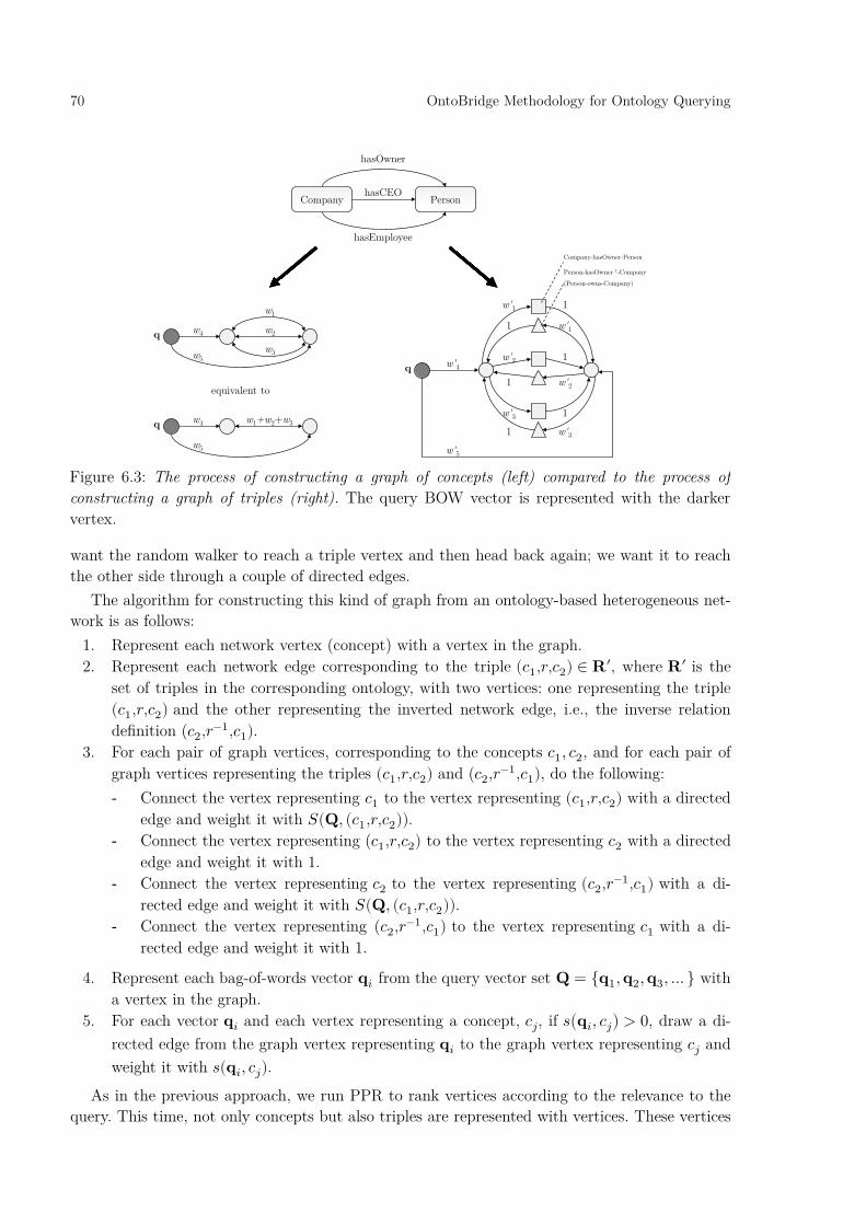
70 OntoBridge Methodology for Ontology Querying
want the random walker to reach a triple vertex and then head back again; we want it to reach the other side through a couple of directed edges.
The algorithm for constructing this kind of graph from an ontology-based heterogeneous net-work is as follows:
1. Represent each network vertex (concept) with a vertex in the graph. 2. Represent each network edge corresponding to the triple (𝑐𝑐1,𝑟𝑟,𝑐𝑐2) ∈ 𝐑𝐑′, where 𝐑𝐑′ is the
set of triples in the corresponding ontology, with two vertices: one representing the triple (𝑐𝑐1,𝑟𝑟,𝑐𝑐2) and the other representing the inverted network edge, i.e., the inverse relation definition (𝑐𝑐2,𝑟𝑟−1,𝑐𝑐1).
3. For each pair of graph vertices, corresponding to the concepts 𝑐𝑐1, 𝑐𝑐2, and for each pair of graph vertices representing the triples (𝑐𝑐1,𝑟𝑟,𝑐𝑐2) and (𝑐𝑐2,𝑟𝑟−1,𝑐𝑐1), do the following: - Connect the vertex representing 𝑐𝑐1 to the vertex representing (𝑐𝑐1,𝑟𝑟,𝑐𝑐2) with a directed
edge and weight it with 𝑆𝑆(𝐐𝐐, (𝑐𝑐1,𝑟𝑟,𝑐𝑐2)). - Connect the vertex representing (𝑐𝑐1,𝑟𝑟,𝑐𝑐2) to the vertex representing 𝑐𝑐2 with a directed
edge and weight it with 1. - Connect the vertex representing 𝑐𝑐2 to the vertex representing (𝑐𝑐2,𝑟𝑟−1,𝑐𝑐1) with a di-
rected edge and weight it with 𝑆𝑆(𝐐𝐐, (𝑐𝑐1,𝑟𝑟,𝑐𝑐2)). - Connect the vertex representing (𝑐𝑐2,𝑟𝑟−1,𝑐𝑐1) to the vertex representing 𝑐𝑐1 with a di-
rected edge and weight it with 1.
4. Represent each bag-of-words vector 𝐪𝐪𝑖𝑖 from the query vector set 𝐐𝐐 = {𝐪𝐪1, 𝐪𝐪2, 𝐪𝐪3,…} with a vertex in the graph.
5. For each vector 𝐪𝐪𝑖𝑖 and each vertex representing a concept, 𝑐𝑐𝑗𝑗, if 𝑠𝑠�𝐪𝐪𝑖𝑖, 𝑐𝑐𝑗𝑗� > 0, draw a di-rected edge from the graph vertex representing 𝐪𝐪𝑖𝑖 to the graph vertex representing 𝑐𝑐𝑗𝑗 and weight it with 𝑠𝑠(𝐪𝐪𝑖𝑖, 𝑐𝑐𝑗𝑗).
As in the previous approach, we run PPR to rank vertices according to the relevance to the query. This time, not only concepts but also triples are represented with vertices. These vertices
Figure 6.3: The process of constructing a graph of concepts (left) compared to the process of constructing a graph of triples (right). The query BOW vector is represented with the darker vertex.
Company Person
hasOwner
hasCEO
hasEmployee
q
w1
w2
w3
equivalent to
q w1+w2+w3
w4
w5
w4
w5
q w'4
w'5
w'1
Company-hasOwner-Person
1 w'1
w'2 1
1 w'2
w'3 1
1 w'3
Person-hasOwner–1-Company
1
(Person-owns-Company)

OntoBridge Methodology for Ontology Querying 71
also receive ranking scores, which in effect allows us to also rank triples. Note that a triple (𝑐𝑐1,𝑟𝑟,𝑐𝑐2) ∈ 𝐑𝐑′ accumulates the ranking score in two different vertices: in the vertex representing (𝑐𝑐1,𝑟𝑟,𝑐𝑐2) and in the vertex representing (𝑐𝑐2,𝑟𝑟−1,𝑐𝑐1). It is thus necessary to sum the ranking scores of these two vertices to obtain the ranking score of the triple.
6.3 Software availability As opposed to the TEHmINe methodology which is implemented in LATINO and partly as a set of components in ClowdFlows/TextFlows, the ontology querying workflow shown in Figure 3.4 will potentially be implemented in ClowdFlows as part of future work. Nevertheless, the workflow is currently implemented as part of Visual OntoBridge and is as such available in a publicly accessible Git repository (Online reference [17]). Visual OntoBridge is also available as a Windows executable (Online reference [18]).

73
7 VideoLectures.net Categorization Use Case
This chapter presents the first use case. The aim was to develop an automatic categorization tool for video lectures hosted at VideoLectures.net. We employed TEHmINe to combine textual data and structure from a text-enriched heterogeneous information network formed out of the available VideoLectures.net data. We show that the use of the methodology results in fast, accurate, memory-efficient, and robust classifiers that outperform the standard text mining routine and diffusion kernels from several different aspects. We also present a visualization-guided analysis which reveals that derived graphs with many disconnected components are unable to perform well when not used in combination with other types of data.
7.1 Problem definition The task in the VideoLectures.net use case was to develop a method that can be used to support the categorization of video lectures hosted by VideoLectures.net. VideoLectures.net is one of the world’s largest scientific and educational video web sites, currently hosting more than 17,000 online lectures (April, 2015). The lectures are given by scholars and scientists from different fields of science, at events such as conferences, summer schools, and workshops. Most of the lectures were recorded and post-produced by the VideoLectures.net team. Consequently, all the data has undergone an editorial process. Apart from the lectures produced by VideoLectures.net, several high-profile content providers (such as MIT, CERN, and Yale) also disseminate their content through the VideoLectures.net portal.
The categorizer was initially implemented in February 2009. Automated categorization was required due to the rapid growth of the number of hosted lectures (150–200 lectures were added each month at that time) as well as due to the fact that the categorization taxonomy is rather fine-grained (129 categories in the provided database snapshot). We evaluated our methodology in this use case, confronting it with a typical text mining approach and an approach based on diffusion kernels.
Since most of the video lectures at VideoLectures.net are equipped with titles and descriptions, the baseline categorizer was implemented by using the standard text mining approach based on the bag-of-words representation of documents. Text categorization is a widely researched area due to its value in real-life applications such as indexing of scientific articles, patent categorization, spam filtering, and web page categorization (Sebastiani, 2002).
7.2 Dataset The VideoLectures.net team provided us with a set of 3,520 English lectures, 1,156 of which were manually categorized (data snapshot from November 2008). Each lecture is described with a title, while 2,537 lectures also have a short description. The lectures are categorized into 129 categories. Each lecture can be assigned to more than one category (on average, a categorized lecture is

74 VideoLectures.net Categorization Use Case
categorized into 1.26 categories). There are 2,706 authors in the dataset, 219 events at which the lectures were recorded, and 62,070 portal users’ click streams.
From this data, it is possible to represent lectures, authors, events, and portal users as a heterogeneous information network. In this network, authors are linked to lectures, lectures are linked to events, and portal users are linked to lectures that they viewed. From the available data, we derived the following textual and structural information about video lectures:
1. Each lecture is assigned a text document formed from the title and, if available, extended with the corresponding lecture description (abstract).
2. The structural information of this heterogeneous information network is represented in the form of three weighted graphs in which nodes represent individual video lectures:
(a) Same-event graph. Two nodes are linked if the two corresponding lectures were rec-orded at the same event. The weight of a link is always 1.
(b) Same-author graph. Two nodes are linked if the two corresponding lectures were pre-sented by the same author or authors. A link is weighted by the number of authors the two lectures have in common.
(c) Viewed-together graph. Two nodes are linked if the two corresponding lectures were viewed together by the same portal user or users. A link is weighted by the number of users that viewed both lectures.
7.3 Results of text mining and diffusion kernels We first performed a set of experiments on textual data only, by following a typical text mining approach. In addition, we employed diffusion kernels (DK) for classifying lectures according to their structural contexts.
In the text mining experiments, each lecture was assigned a text document formed from the title and, if available, extended with the corresponding description. We represented the docu-ments as normalized BOW vectors. In the first set of experiments, we tested several different BOW construction settings. We varied the type of weights (TF or TF-IDF), maximum n-gram length (𝑛𝑛), minimum required term frequency (𝑚𝑚𝑖𝑖𝑛𝑛-𝑓𝑓𝑟𝑟𝑒𝑒𝑞𝑞) and cut-off percentage1 (𝑐𝑐𝐶𝐶𝑡𝑡-𝑙𝑙𝑓𝑓𝑓𝑓). We employed the nearest centroid classifier (for details, see Section 4.1.3) in the first set of experi-ments and performed 10-fold cross-validation on the manually categorized lectures. We performed flat classification as suggested in (Grobelnik and Mladenić, 2005). We measured the classification accuracy on the top 1, 3, 5, and 10 categories predicted by the classifier.
The results are given in Table 7.1. We can see that the TF-IDF weighting scheme outperforms the TF weighting scheme, that taking bigrams into account in addition to unigrams improves the performance, and that it is beneficial to process only those terms that occur in the document collection at least twice. We therefore used Setting 5 in all our subsequent experiments involving BOW vector representation. 1 The cut-off percentage allows us to prune off tails of BOW vectors. In the pruning process, we remove the com-
ponents with the smallest weights so that their aggregated weight accounts for the specified share (i.e., cut-off) of the overall weight.
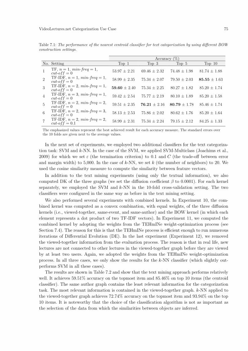
VideoLectures.net Categorization Use Case 75
In the next set of experiments, we employed two additional classifiers for the text categoriza-tion task: SVM and 𝑘𝑘-NN. In the case of the SVM, we applied SVM-Multiclass (Joachims et al., 2009) for which we set 𝜀𝜀 (the termination criterion) to 0.1 and 𝐶𝐶 (the trade-off between error and margin width) to 5,000. In the case of 𝑘𝑘-NN, we set 𝑘𝑘 (the number of neighbors) to 20. We used the cosine similarity measure to compute the similarity between feature vectors.
In addition to the text mining experiments (using only the textual information), we also computed DK of the three graphs (we set the diffusion coefficient 𝛽𝛽 to 0.0001). For each kernel separately, we employed the SVM and 𝑘𝑘-NN in the 10-fold cross-validation setting. The two classifiers were configured in the same way as before in the text mining setting.
We also performed several experiments with combined kernels. In Experiment 10, the com-bined kernel was computed as a convex combination, with equal weights, of the three diffusion kernels (i.e., viewed-together, same-event, and same-author) and the BOW kernel (in which each element represents a dot product of two TF-IDF vectors). In Experiment 11, we computed the combined kernel by adopting the weights from the TEHmINe weight-optimization process (see Section 7.4). The reason for this is that the TEHmINe process is efficient enough to run numerous iterations of Differential Evolution (DE). In the last experiment (Experiment 12), we removed the viewed-together information from the evaluation process. The reason is that in real life, new lectures are not connected to other lectures in the viewed-together graph before they are viewed by at least two users. Again, we adopted the weights from the TEHmINe weight-optimization process. In all three cases, we only show the results for the 𝑘𝑘-NN classifier (which slightly out-performs SVM in all these cases).
The results are shown in Table 7.2 and show that the text mining approach performs relatively well. It achieves 59.51% accuracy on the topmost item and 85.46% on top 10 items (the centroid classifier). The same author graph contains the least relevant information for the categorization task. The most relevant information is contained in the viewed-together graph. 𝑘𝑘-NN applied to the viewed-together graph achieves 72.74% accuracy on the topmost item and 93.94% on the top 10 items. It is noteworthy that the choice of the classification algorithm is not as important as the selection of the data from which the similarities between objects are inferred.
Table 7.1: The performance of the nearest centroid classifier for text categorization by using different BOW construction settings.
Accuracy (%) No. Setting Top 1 Top 3 Top 5 Top 10
1 TF, 𝑛𝑛 = 1, 𝑚𝑚𝑖𝑖𝑛𝑛-𝑓𝑓𝑟𝑟𝑒𝑒𝑞𝑞 = 1, 𝑐𝑐𝐶𝐶𝑡𝑡-𝑙𝑙𝑓𝑓𝑓𝑓 = 0 53.97 ± 2.21 69.46 ± 2.32 74.48 ± 1.98 81.74 ± 1.88
2 TF-IDF, 𝑛𝑛 = 1, 𝑚𝑚𝑖𝑖𝑛𝑛-𝑓𝑓𝑟𝑟𝑒𝑒𝑞𝑞 = 1, 𝑐𝑐𝐶𝐶𝑡𝑡-𝑙𝑙𝑓𝑓𝑓𝑓 = 0 58.99 ± 2.35 75.34 ± 2.07 79.50 ± 2.03 85.55 ± 1.63
3 TF-IDF, 𝑛𝑛 = 2, 𝑚𝑚𝑖𝑖𝑛𝑛-𝑓𝑓𝑟𝑟𝑒𝑒𝑞𝑞 = 1, 𝑐𝑐𝐶𝐶𝑡𝑡-𝑙𝑙𝑓𝑓𝑓𝑓 = 0 59.60 ± 2.40 75.34 ± 2.25 80.27 ± 1.82 85.20 ± 1.74
4 TF-IDF, 𝑛𝑛 = 3, 𝑚𝑚𝑖𝑖𝑛𝑛-𝑓𝑓𝑟𝑟𝑒𝑒𝑞𝑞 = 1, 𝑐𝑐𝐶𝐶𝑡𝑡-𝑙𝑙𝑓𝑓𝑓𝑓 = 0 59.42 ± 2.54 75.77 ± 2.19 80.10 ± 1.89 85.20 ± 1.58
5 TF-IDF, 𝑛𝑛 = 2, 𝑚𝑚𝑖𝑖𝑛𝑛-𝑓𝑓𝑟𝑟𝑒𝑒𝑞𝑞 = 2, 𝑐𝑐𝐶𝐶𝑡𝑡-𝑙𝑙𝑓𝑓𝑓𝑓 = 0 59.51 ± 2.35 76.21 ± 2.16 80.79 ± 1.78 85.46 ± 1.74
6 TF-IDF, 𝑛𝑛 = 2, 𝑚𝑚𝑖𝑖𝑛𝑛-𝑓𝑓𝑟𝑟𝑒𝑒𝑞𝑞 = 3, 𝑐𝑐𝐶𝐶𝑡𝑡-𝑙𝑙𝑓𝑓𝑓𝑓 = 0 58.13 ± 2.53 75.86 ± 2.02 80.62 ± 1.76 85.20 ± 1.64
7 TF-IDF, 𝑛𝑛 = 2, 𝑚𝑚𝑖𝑖𝑛𝑛-𝑓𝑓𝑟𝑟𝑒𝑒𝑞𝑞 = 2, 𝑐𝑐𝐶𝐶𝑡𝑡-𝑙𝑙𝑓𝑓𝑓𝑓 = 0.1 58.99 ± 2.31 75.34 ± 2.24 79.15 ± 2.12 84.25 ± 1.33
The emphasized values represent the best achieved result for each accuracy measure. The standard errors over the 10 folds are given next to the average values.

76 VideoLectures.net Categorization Use Case
The results of the combined kernels show that weighting all types of data equally does not produce the best results. The accuracy falls in comparison with Experiments 4 and 5 which use the also-watched diffusion kernel alone. Even though the weights in Experiment 11 are adopted from the TEHmINe weight-optimization process, the results are substantially better than those using equal weighting. The combined kernel in Experiment 11 still performs worse than the viewed-together diffusion kernel.
7.4 TEHmINe results In the next set of experiments, we applied the proposed TEHmINe methodology. The results are presented in Table 7.3.
The first nine experiments summarized in Table 7.3 were performed by employing the proposed methodology on each graph separately. As before, we performed 10-fold cross-validation on the manually categorized lectures and employed the centroid classifier, SVM-Multiclass, and 𝑘𝑘-NN for the categorization task (we used the same parameter values as before). We set the PageRank damping factor to 0.4 when computing the structural-context feature vectors.
In the last three experiments summarized in Table 7.3, we employed the data fusion method explained in Section 5.2.4. In Experiment 10, all types of data were weighted equally (i.e., BOW, viewed-together, same-event, and same-author). We only show the results for the nearest centroid classifier (which outperforms SVM and 𝑘𝑘-NN in these cases). In Experiment 11, we employed DE to directly optimize the target evaluation metrics. The objective function was computed in an inner 10-fold cross-validation loop for each evaluation metric separately. We only employed the centroid classifier in this setting as it is fast enough to allow for numerous iterations required for
Table 7.2: The results of the selected text classification algorithms and diffusion kernels.
Accuracy (%) No. Setting Top 1 Top 3 Top 5 Top 10 1 Text mining, SVM 59.16 ± 2.34 73.09 ± 1.82 78.28 ± 1.55 82.96 ± 1.32 2 Text mining, 𝑘𝑘-NN 58.47 ± 2.07 72.74 ± 1.97 78.28 ± 2.08 83.91 ± 1.55 3 Text mining, NCC 59.51 ± 2.35 76.21 ± 2.16 80.79 ± 1.78 85.46 ± 1.74 4 DK, viewed-together, SVM 70.75 ± 1.93 86.94 ± 1.55 90.92 ± 1.30 93.68 ± 1.25 5 DK, viewed-together, 𝑘𝑘-NN 72.74 ± 1.51 87.80 ± 1.30 90.83 ± 1.05 93.94 ± 0.68 6 DK, same-event, SVM 32.00 ± 1.45 49.04 ± 1.53 54.67 ± 1.30 58.65 ± 1.12 7 DK, same-event, 𝑘𝑘-NN 31.92 ± 1.38 47.66 ± 1.64 53.37 ± 1.52 61.07 ± 1.32 8 DK, same-author, SVM 18.94 ± 1.00 27.51 ± 1.06 31.22 ± 1.09 36.24 ± 1.25 9 DK, same-author, 𝑘𝑘-NN 19.81 ± 1.05 31.74 ± 1.18 36.24 ± 1.42 43.59 ± 1.31
10 DK, combined, equal weights, 𝑘𝑘-NN 59.07 ± 2.11 73.87 ± 2.02 78.89 ± 2.01 85.03 ± 1.41
11 DK, combined, optimized weights*, 𝑘𝑘-NN 66.08 ± 2.06 81.40 ± 1.47 84.25 ± 1.71 90.92 ± 1.17
12 DK, combined without viewed-together, optimized weights*, 𝑘𝑘-NN
58.64 ± 2.07 73.09 ± 1.94 78.54 ± 2.03 84.25 ± 1.48
The emphasized values represent the best achieved result for each accuracy measure in each group of experiments. The standard errors over the 10 folds are given next to the average values. *The weights are adopted from the TEHmINe weight-optimization process (see Section 7.4).

VideoLectures.net Categorization Use Case 77
the stochastic optimizer to find a good solution. The weights, determined by DE, averaged over the 10 folds for each evaluation metric separately, are given in Table 7.4.
In the last experiment (Experiment 12), we removed the viewed-together information from the evaluation process. The reason is that in real life, new lectures are not connected to other lectures in the viewed-together graph because they were not yet viewed by any user. Again, we employed DE in an inner 10-fold cross-validation loop for each evaluation metric separately. The resulting weights are given in Table 7.5.
From the results of the first nine experiments, we can confirm that the most relevant infor-mation is contained in the viewed-together graph. The centroid classifier applied to the viewed-together graph exhibits 74.91% accuracy on the topmost item and 95.33% on the top 10 items. We can also confirm that the choice of the classification algorithm is not as important as the selection of the data from which the similarities between objects are inferred. Even so, the cen-troid classifier does outperform the SVM and the 𝑘𝑘-NN on the top 10 items and in the case of the viewed-together graph, also on the topmost item. The centroid classifier is outperformed by the other two classifiers on the topmost item in the case of the same-event and same-author graphs.
The results of Experiment 10 show that weighting all types of data equally does not produce the best results. The accuracy falls in comparison with exploiting the viewed-together graph alone. The optimized weights indeed yield the best results (Experiment 11) and improve the categorization performance (compared to exploiting the viewed-together graph alone: 77.68 vs.
Table 7.3: The results of employing the proposed methodology.
Accuracy (%) No. Setting Top 1 Top 3 Top 5 Top 10 1 Viewed-together, SVM 70.41 ± 1.45 85.46 ± 1.68 89.71 ± 1.52 93.60 ± 1.41 2 Viewed-together, 𝑘𝑘-NN 70.75 ± 1.71 84.60 ± 1.65 89.36 ± 1.26 93.34 ± 0.98 3 Viewed-together, NCC 74.91 ± 1.82 89.01 ± 1.14 92.13 ± 1.07 95.33 ± 1.02 4 Same-event, SVM 31.74 ± 1.00 50.17 ± 1.09 55.97 ± 1.08 59.95 ± 1.03 5 Same-event, 𝑘𝑘-NN 32.34 ± 1.57 50.43 ± 1.32 55.96 ± 1.11 64.79 ± 0.99 6 Same-event, NCC 27.59 ± 1.16 46.62 ± 1.29 53.63 ± 1.37 65.05 ± 0.93 7 Same-author, SVM 15.83 ± 0.92 24.22 ± 1.02 27.33 ± 1.07 33.04 ± 1.00 8 Same-author, 𝑘𝑘-NN 15.48 ± 0.88 23.70 ± 0.87 27.94 ± 0.91 32.52 ± 1.23 9 Same-author, NCC 14.79 ± 0.73 25.52 ± 0.75 31.74 ± 0.82 42.73 ± 1.60 10 Combined, equal weights, NCC 66.25 ± 1.94 83.12 ± 1.09 86.93 ± 1.11 93.08 ± 1.08 11 Combined, DE, NCC 77.68 ± 1.30 90.66 ± 1.29 93.34 ± 0.92 95.85 ± 0.75 12 Without viewed-together, NCC 62.97 ± 2.10 79.06 ± 1.86 84.07 ± 1.28 89.10 ± 1.18 The emphasized values represent the best achieved result for each accuracy measure in each group of experiments. The standard errors over the 10 folds are given next to the average values.
Table 7.4: The weights computed in the optimization process in Experiment 11.
Average weights Accuracy measure Viewed together Same event Same author BOW Top 1 0.9310 ± 0.0038 0.0057 ± 0.0014 0.0049 ± 0.0019 0.0585 ± 0.0045 Top 3 0.8839 ± 0.0079 0.0455 ± 0.0065 0.0096 ± 0.0028 0.0611 ± 0.0035 Top 5 0.7607 ± 0.0195 0.0648 ± 0.0093 0.0892 ± 0.0112 0.0853 ± 0.0073 Top 10 0.7931 ± 0.0391 0.0505 ± 0.0168 0.0968 ± 0.0336 0.0596 ± 0.0061 The standard errors over the 10 folds are given next to the average values.

78 VideoLectures.net Categorization Use Case
74.91% on the topmost item, 95.85 vs. 95.33% on the top 10 items). This is also the case when the viewed-together information is not present in the test set (Experiment 12). The classifier is able to exploit the remaining data and exhibit accuracies that are higher than those achieved by resorting to text mining alone (62.97 vs. 59.51% on the topmost item, 89.10 vs. 85.46% on the top 10 items). A classifier based on combined feature vectors is not only more accurate but is also robust to missing a certain type of data in the test examples.
When comparing the single-graph TEHmINe approaches (Table 7.3, Experiments 1 to 9) to the single-kernel DK approaches (Table 7.2, Experiments 4 to 9), we can see that the centroid
Table 7.5: The weights computed in the optimization process in Experiment 12.
Average weights Accuracy measure Same event Same author BOW Top 1 0.3796 ± 0.0191 0.1852 ± 0.0310 0.4352 ± 0.0202 Top 3 0.3601 ± 0.0181 0.0899 ± 0.0301 0.5500 ± 0.0350 Top 5 0.3424 ± 0.0259 0.2339 ± 0.0505 0.4237 ± 0.0313 Top 10 0.2606 ± 0.0361 0.4146 ± 0.0683 0.3247 ± 0.0460 The standard errors over the 10 folds are given next to the average values.
Table 7.6: The summary of all the results.
Accuracy (%) Ref. Setting Top 1 Top 3 Top 5 Top 10 T7.2.3 Text mining, NCC 59.51 ± 2.35 76.21 ± 2.16 80.79 ± 1.78 85.46 ± 1.74
T7.2.5 DK, viewed-together, 𝑘𝑘-NN 72.74 ± 1.51 87.80 ± 1.30 90.83 ± 1.05 93.94 ± 0.68
T7.3.3 TEHmINe, viewed-to-gether, NCC 74.91 ± 1.82 89.01 ± 1.14 92.13 ± 1.07 95.33 ± 1.02
T7.2.6 DK, same-event, SVM 32.00 ± 1.45 49.04 ± 1.53 54.67 ± 1.30 58.65 ± 1.12 T7.3.6 TEHmINe, same-event,
NCC 27.59 ± 1.16 46.62 ± 1.29 53.63 ± 1.37 65.05 ± 0.93
T7.2.9 DK, same-author, 𝑘𝑘-NN 19.81 ± 1.05 31.74 ± 1.18 36.24 ± 1.42 43.59 ± 1.31
T7.3.9 TEHmINe, same-author, NCC 14.79 ± 0.73 25.52 ± 0.75 31.74 ± 0.82 42.73 ± 1.60
T7.2.10 DK, combined, equal weights, 𝑘𝑘-NN 59.07 ± 2.11 73.87 ± 2.02 78.89 ± 2.01 85.03 ± 1.41
T7.3.10 TEHmINe, combined, equal weights, NCC 66.25 ± 1.94 83.12 ± 1.09 86.93 ± 1.11 93.08 ± 1.08
T7.2.11 DK, combined, optimized weights, 𝑘𝑘-NN 66.08 ± 2.06 81.40 ± 1.47 84.25 ± 1.71 90.92 ± 1.17
T7.3.11 TEHmINe, combined, opti-mized weights, NCC 77.68 ± 1.30 90.66 ± 1.29 93.34 ± 0.92 95.85 ± 0.75
T7.2.12 DK, combined without viewed-together, optimized weights, 𝑘𝑘-NN
58.64 ± 2.07 73.09 ± 1.94 78.54 ± 2.03 84.25 ± 1.48
T7.3.12 TEHmINe, combined with-out viewed-together, opti-mized weights, NCC
62.97 ± 2.10 79.06 ± 1.86 84.07 ± 1.28 89.10 ± 1.18
This table summarizes the results from Tables 7.2 and 7.3, respectively. The original tables (together with the ex-periment number) are referenced in the first column. The emphasized values represent the best achieved result for each accuracy measure in each group of experiments. The standard errors over the 10 folds are given next to the average values.
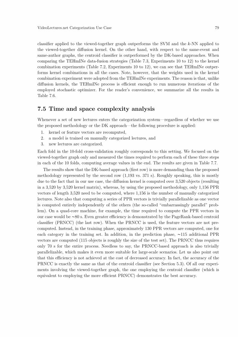
VideoLectures.net Categorization Use Case 79
classifier applied to the viewed-together graph outperforms the SVM and the 𝑘𝑘-NN applied to the viewed-together diffusion kernel. On the other hand, with respect to the same-event and same-author graphs, the centroid classifier is outperformed by the DK-based approaches. When comparing the TEHmINe data-fusion strategies (Table 7.3, Experiments 10 to 12) to the kernel combination experiments (Table 7.2, Experiments 10 to 12), we can see that TEHmINe outper-forms kernel combinations in all the cases. Note, however, that the weights used in the kernel combination experiment were adopted from the TEHmINe experiments. The reason is that, unlike diffusion kernels, the TEHmINe process is efficient enough to run numerous iterations of the employed stochastic optimizer. For the reader’s convenience, we summarize all the results in Table 7.6.
7.5 Time and space complexity analysis Whenever a set of new lectures enters the categorization system—regardless of whether we use the proposed methodology or the DK approach—the following procedure is applied:
1. kernel or feature vectors are recomputed, 2. a model is trained on manually categorized lectures, and 3. new lectures are categorized.
Each fold in the 10-fold cross-validation roughly corresponds to this setting. We focused on the viewed-together graph only and measured the times required to perform each of these three steps in each of the 10 folds, computing average values in the end. The results are given in Table 7.7.
The results show that the DK-based approach (first row) is more demanding than the proposed methodology represented by the second row (1,193 vs. 371 s). Roughly speaking, this is mostly due to the fact that in our use case, the diffusion kernel is computed over 3,520 objects (resulting in a 3,520 by 3,520 kernel matrix), whereas, by using the proposed methodology, only 1,156 PPR vectors of length 3,520 need to be computed, where 1,156 is the number of manually categorized lectures. Note also that computing a series of PPR vectors is trivially parallelizable as one vector is computed entirely independently of the others (the so-called “embarrassingly parallel” prob-lem). On a quad-core machine, for example, the time required to compute the PPR vectors in our case would be ∼80 s. Even greater efficiency is demonstrated by the PageRank-based centroid classifier (PRNCC) (the last row). When the PRNCC is used, the feature vectors are not pre-computed. Instead, in the training phase, approximately 130 PPR vectors are computed, one for each category in the training set. In addition, in the prediction phase, ∼115 additional PPR vectors are computed (115 objects is roughly the size of the test set). The PRNCC thus requires only 70 s for the entire process. Needless to say, the PRNCC-based approach is also trivially parallelizable, which makes it even more suitable for large-scale scenarios. Let us also point out that this efficiency is not achieved at the cost of decreased accuracy. In fact, the accuracy of the PRNCC is exactly the same as that of the centroid classifier (see Section 5.3). Of all our experi-ments involving the viewed-together graph, the one employing the centroid classifier (which is equivalent to employing the more efficient PRNCC) demonstrates the best accuracy.
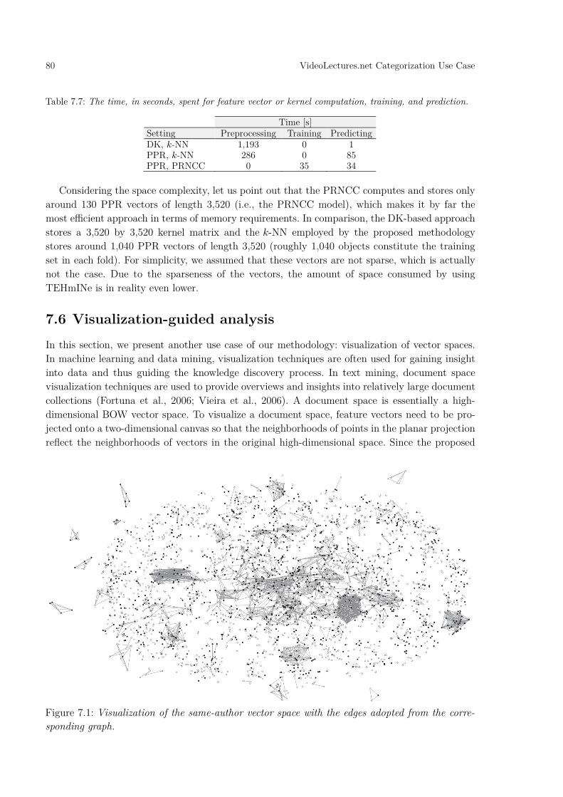
80 VideoLectures.net Categorization Use Case
Considering the space complexity, let us point out that the PRNCC computes and stores only around 130 PPR vectors of length 3,520 (i.e., the PRNCC model), which makes it by far the most efficient approach in terms of memory requirements. In comparison, the DK-based approach stores a 3,520 by 3,520 kernel matrix and the 𝑘𝑘-NN employed by the proposed methodology stores around 1,040 PPR vectors of length 3,520 (roughly 1,040 objects constitute the training set in each fold). For simplicity, we assumed that these vectors are not sparse, which is actually not the case. Due to the sparseness of the vectors, the amount of space consumed by using TEHmINe is in reality even lower.
7.6 Visualization-guided analysis
In this section, we present another use case of our methodology: visualization of vector spaces. In machine learning and data mining, visualization techniques are often used for gaining insight into data and thus guiding the knowledge discovery process. In text mining, document space visualization techniques are used to provide overviews and insights into relatively large document collections (Fortuna et al., 2006; Vieira et al., 2006). A document space is essentially a high-dimensional BOW vector space. To visualize a document space, feature vectors need to be pro-jected onto a two-dimensional canvas so that the neighborhoods of points in the planar projection reflect the neighborhoods of vectors in the original high-dimensional space. Since the proposed
Table 7.7: The time, in seconds, spent for feature vector or kernel computation, training, and prediction.
Time [s] Setting Preprocessing Training Predicting DK, 𝑘𝑘-NN 1,193 0 1 PPR, 𝑘𝑘-NN 286 0 85 PPR, PRNCC 0 35 34
Figure 7.1: Visualization of the same-author vector space with the edges adopted from the corre-sponding graph.

VideoLectures.net Categorization Use Case 81
methodology enables us to convert graphs into BOW-like vectors, we can visualize these graphs by using one of the available document space visualization techniques. Even more, we can visu-alize any “fusion” of feature vectors obtained by following the proposed methodology. We will employ the document space visualization technique based on least-square meshes (Sorkine and Cohen-Or, 2004; Vieira et al., 2006)—more specifically, the implementation thoroughly presented in (Grčar et al., 2010)—to demonstrate how visualized vector spaces can provide valuable insights. Specifically, we will explain why the same-author graph, even though based on a solid intuition that “a scientist normally sticks to his field of science”, demonstrates such poor performance when used for categorization. From this same perspective, we will examine the same-event graph and look for the key difference between the same-author and same-event graphs on one hand and the viewed-together graph on the other.
Figure 7.1 shows the visualization of the same-author vector space with the edges adopted from the same-author graph. We can clearly see that we are dealing with many disconnected components. Each component corresponds to a group of lectures presented by the same author or several authors of which each collaborated with at least one other author from the group on at least one paper (lecture). The black dots in the visualization represent the lectures that were manually categorized (ground truth) and the white dots represent the uncategorized lectures. Note that (1) only the categorized lectures (black dots) participate in the 10-fold cross-validation process and, (2) given a categorized lecture from a particular component, only the lectures from the same component participate as features in the feature vector of this categorized lecture. Let us now consider a component with one single categorized lecture (black dot). When such a cate-gorized lecture is part of the test set in the cross-validation process, the corresponding feature vector is orthogonal to every feature vector in the training set (note that only the categorized lectures constitute the training set). This means that it is not possible to categorize it due to the lack of information caused by the sparseness of the same-author graph. In general, the smaller the number of categorized lectures in a component, the bigger the chance that they will all
Figure 7.2: Visualization of the same-event vector space with the edges adopted from the corre-sponding graph.

82 VideoLectures.net Categorization Use Case
constitute the same fold in the cross-validation setting, which results in the inability to classify any of them when the corresponding fold forms the test set. From this, we can conclude that having many disconnected components containing low numbers of categorized lectures leads to a poor categorization performance.
Figures 7.2 and 7.3 show the visualization of the same-event and viewed-together vector space, respectively. We can see that (1) the viewed-together graph contains less disconnected compo-nents than the same-event graph, which contains less disconnected components than the same-author graph (note that each single disconnected dot also represents a disconnected component), (2) the viewed-together graph contains one large component containing nearly all the categorized lectures, and (3) the components in the same-event graph are larger than those in the same-author graph and thus each of them has the potential of containing a larger number of categorized lectures.
To make sure that these observations are not merely “visual artifacts”, we computed the number of disconnected components and the number of components containing a certain number of categorized lectures in each of the three graphs. The results for the same-author and same-event graphs are shown in Figures 7.4 and 7.5, respectively. The viewed-together graph consists of 99 disconnected components of which 1 contains 1,155 categorized lectures, 1 contains 1 cate-gorized lecture, and 97 contain no categorized lectures.
The charts in Figures 7.4 and 7.5 clearly support our claims. The same-author graph contains the largest number of components (i.e., 2,519) and a relatively large number of components that contain low numbers of categorized lectures. The same-event graph contains roughly 10 times less components and also the number of components containing low numbers of categorized lec-tures is much lower. If we look at the statistics of the viewed-together graph, we see that it contains only one disconnected categorized lecture that is orthogonal to the training set in the
Figure 7.3: Visualization of the viewed-together vector space with the edges adopted from the corresponding graph.

VideoLectures.net Categorization Use Case 83
cross-validation process. From this perspective, the viewed-together graph exhibits the most ap-propriate structure, followed by the same-event, and same-author graphs. This is also clearly reflected in the empirical studies presented in Section 7.4.
Figure 7.4: The number of disconnected components and the number of components containing a certain number of categorized lectures for the same-author graph.
Figure 7.5: The number of disconnected components and the number of components containing a certain number of categorized lectures for the same-event graph.
1643
760
56 29 11 7 4 2 1 1 1 2 1 1
0 1 2 3 4 5 6 7 8 9 10 11 15 16
Num
ber
of c
ompo
nent
s
Number of categorized lectures
Same-author(2,519 components)
63
33
2112 10 10 7 9 6 4
8 6 5 5 4 1 4 2 1 2 1 2 1 2 1 1 1 1
0 1 2 3 4 5 6 7 8 9 10 11 12 13 14 15 16 17 19 21 22 23 25 26 27 28 31 34
Num
ber
of c
ompo
nent
s
Number of categorized lectures
Same-event(223 components)
84 Ontology Querying Use Case
8 Ontology Querying Use Case
In the following sections, we evaluate the ontology querying methodology for the task of creating semantic annotations in the geospatial domain. Semantic annotations are formal, machine-read-able descriptions that enable efficient search and browse through resources, as well as efficient composition and execution of web services. In this work, the semantic annotation is defined as a set of interlinked ontology elements associated with the resource being annotated (see Section 3.1.2 for a motivating example). In our setting, the task is to annotate schemas of Web Feature Services (WFS). WFS is an Open Geospatial Consortium (OGC) standard that defines an inter-face for querying and editing geographic features, such as roads or lake outlines (Online reference [12]).
The ontology querying methodology was derived from the general-purpose TEHmINe meth-odology. Similarly to the TEHmINe workflow, the ontology querying workflow starts with loading a TEHIN. In this case, the TEHIN represents a grounded ontology. The term “grounded” in this context means that every ontology entity of interest is enriched with a set of documents describing, talking about, or otherwise being related to this entity. In Chapter 6, we already discussed the idea of grounding and explained how an ontology can be viewed as a TEHIN. In addition, we proposed two techniques for converting an ontology-based TEHIN to a homogeneous graph, which is a necessary step in the proposed ontology querying methodology. In the following sections, we compare the use of the ontology querying methodology to the text mining approach that does not take the ontology structure into account.
8.1 Experimental setting In this section, we present the dataset, gold standard, and evaluation metric that we use in our experimental setting. Since the experimental setting has many different parameters, we follow the outcomes of Grčar et al. (2009b) and employ the settings already presented in Section 6.1.2. In addition, we employ the usual way of converting documents into bags-of-words. We eliminate stop words, apply stemming, identify word bigrams, and compute normalized TF-IDF vectors. We take into account only words and bigrams that occur at least 5 times in the entire corpus. From each TF-IDF vector, prior to normalization, we remove the low weights that collectively constitute 20% of the sum of all the weights in the vector.
8.1.1 Dataset and gold standard
For the experiments, we acquired an ontology and a set of Web Feature Services (WFS’s). Each WFS was accompanied with several sets of user queries.
The ontology was provided by the University of Münster. It is an early version of the SWING ontology (Andrei et al., 2008). It contains 332 concepts, 141 relations, and 4,362 domain-relation-
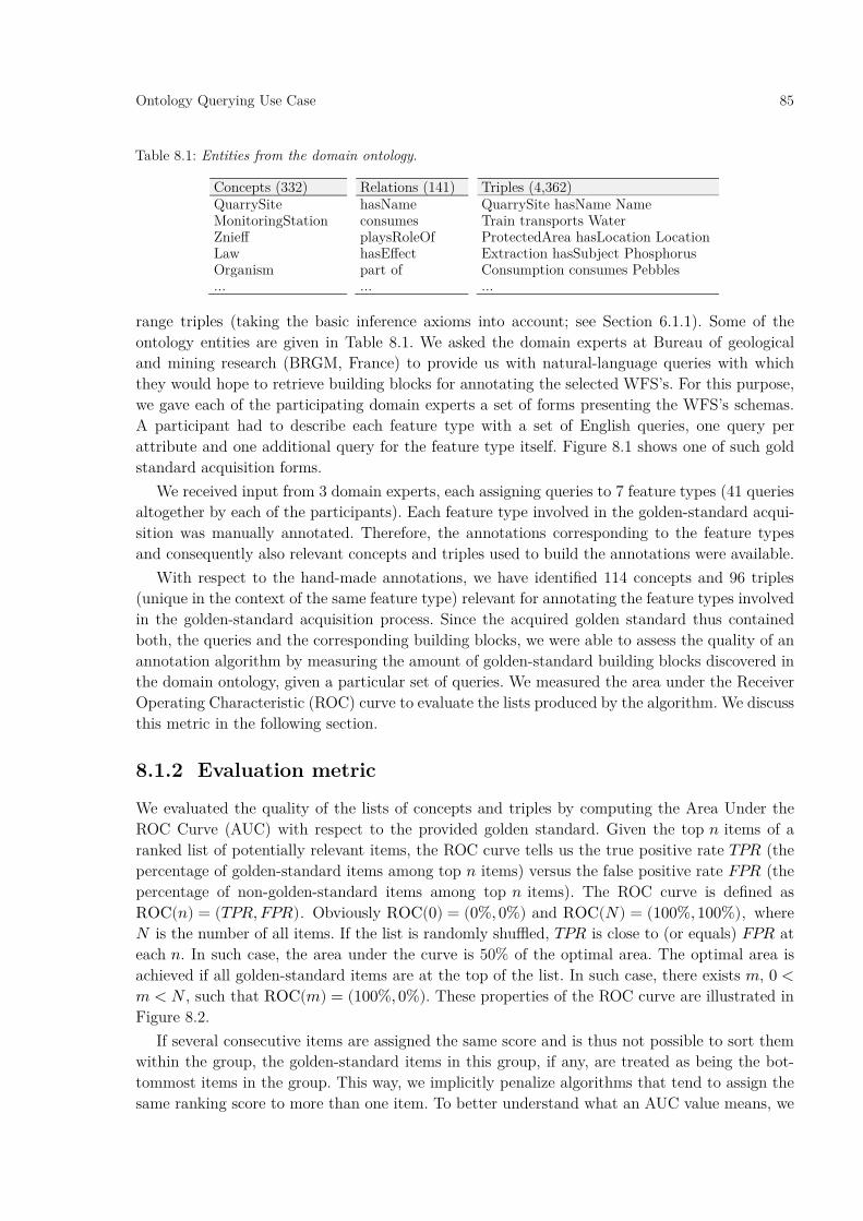
Ontology Querying Use Case 85
range triples (taking the basic inference axioms into account; see Section 6.1.1). Some of the ontology entities are given in Table 8.1. We asked the domain experts at Bureau of geological and mining research (BRGM, France) to provide us with natural-language queries with which they would hope to retrieve building blocks for annotating the selected WFS’s. For this purpose, we gave each of the participating domain experts a set of forms presenting the WFS’s schemas. A participant had to describe each feature type with a set of English queries, one query per attribute and one additional query for the feature type itself. Figure 8.1 shows one of such gold standard acquisition forms.
We received input from 3 domain experts, each assigning queries to 7 feature types (41 queries altogether by each of the participants). Each feature type involved in the golden-standard acqui-sition was manually annotated. Therefore, the annotations corresponding to the feature types and consequently also relevant concepts and triples used to build the annotations were available.
With respect to the hand-made annotations, we have identified 114 concepts and 96 triples (unique in the context of the same feature type) relevant for annotating the feature types involved in the golden-standard acquisition process. Since the acquired golden standard thus contained both, the queries and the corresponding building blocks, we were able to assess the quality of an annotation algorithm by measuring the amount of golden-standard building blocks discovered in the domain ontology, given a particular set of queries. We measured the area under the Receiver Operating Characteristic (ROC) curve to evaluate the lists produced by the algorithm. We discuss this metric in the following section.
8.1.2 Evaluation metric
We evaluated the quality of the lists of concepts and triples by computing the Area Under the ROC Curve (AUC) with respect to the provided golden standard. Given the top 𝑛𝑛 items of a ranked list of potentially relevant items, the ROC curve tells us the true positive rate 𝑇𝑇𝑃𝑃𝑇𝑇 (the percentage of golden-standard items among top 𝑛𝑛 items) versus the false positive rate 𝑇𝑇𝑃𝑃𝑇𝑇 (the percentage of non-golden-standard items among top 𝑛𝑛 items). The ROC curve is defined as ROC(𝑛𝑛) = (𝑇𝑇𝑃𝑃𝑇𝑇, 𝑇𝑇𝑃𝑃𝑇𝑇) . Obviously ROC(0) = (0%, 0%) and ROC(𝑁𝑁) = (100%, 100%) , where 𝑁𝑁 is the number of all items. If the list is randomly shuffled, 𝑇𝑇𝑃𝑃𝑇𝑇 is close to (or equals) 𝑇𝑇𝑃𝑃𝑇𝑇 at each 𝑛𝑛. In such case, the area under the curve is 50% of the optimal area. The optimal area is achieved if all golden-standard items are at the top of the list. In such case, there exists 𝑚𝑚, 0 <𝑚𝑚 < 𝑁𝑁 , such that ROC(𝑚𝑚) = (100%, 0%). These properties of the ROC curve are illustrated in Figure 8.2.
If several consecutive items are assigned the same score and is thus not possible to sort them within the group, the golden-standard items in this group, if any, are treated as being the bot-tommost items in the group. This way, we implicitly penalize algorithms that tend to assign the same ranking score to more than one item. To better understand what an AUC value means, we
Table 8.1: Entities from the domain ontology.
Concepts (332) Relations (141) Triples (4,362) QuarrySite hasName QuarrySite hasName Name MonitoringStation consumes Train transports Water Znieff playsRoleOf ProtectedArea hasLocation Location Law hasEffect Extraction hasSubject Phosphorus Organism part of Consumption consumes Pebbles ... ... ...

86 Ontology Querying Use Case
can interpret it as follows. Suppose that the AUC value is 𝑎𝑎 and the list has 𝑁𝑁 items. One of the possible scenarios is that the correct items are equally distributed amongst the first 2(1 − 𝑎𝑎)𝑁𝑁 items. For example, if AUC is 98% and the list has 5,000 items, the correct items could be equally distributed amongst the first 4% of 5,000 items (i.e., top 200 items). This is, of course, not necessarily the case; it is just a way to quickly assess the practical value of the algorithm being evaluated.
8.2 Evaluation results In the following sections, we discuss the results of the evaluation by assessing the quality of the algorithms and determining a set of good default settings.
Figure 8.1: The gold-standard acquisition form for the feature type “regions”. The feature type (green box) with its attributes (yellow boxes) is visualized in the left-hand side, the corresponding queries, provided by one of the participants, can be seen in the right-hand side of the figure.
Figure 8.2: Basic properties of the ROC curve.
msGeonetry
area
population code
Location of the regionArea of the regionRegionName of the regionPopulation of the regionINSEE identifier of the regionregions
region
Random shuffle
Optimal
n=10n=20
n=30…
50%False positive rate
100%0%
True
pos
itive
rat
e
0%
50%
100%
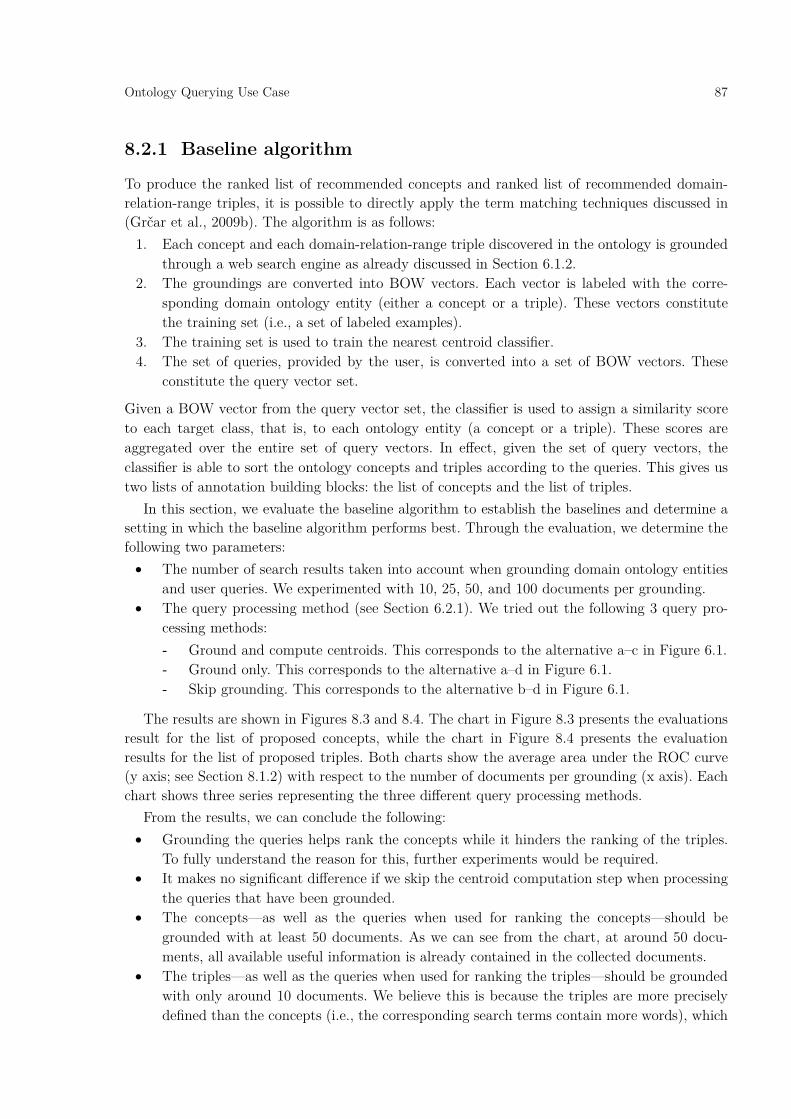
Ontology Querying Use Case 87
8.2.1 Baseline algorithm
To produce the ranked list of recommended concepts and ranked list of recommended domain-relation-range triples, it is possible to directly apply the term matching techniques discussed in (Grčar et al., 2009b). The algorithm is as follows:
1. Each concept and each domain-relation-range triple discovered in the ontology is grounded through a web search engine as already discussed in Section 6.1.2.
2. The groundings are converted into BOW vectors. Each vector is labeled with the corre-sponding domain ontology entity (either a concept or a triple). These vectors constitute the training set (i.e., a set of labeled examples).
3. The training set is used to train the nearest centroid classifier. 4. The set of queries, provided by the user, is converted into a set of BOW vectors. These
constitute the query vector set.
Given a BOW vector from the query vector set, the classifier is used to assign a similarity score to each target class, that is, to each ontology entity (a concept or a triple). These scores are aggregated over the entire set of query vectors. In effect, given the set of query vectors, the classifier is able to sort the ontology concepts and triples according to the queries. This gives us two lists of annotation building blocks: the list of concepts and the list of triples.
In this section, we evaluate the baseline algorithm to establish the baselines and determine a setting in which the baseline algorithm performs best. Through the evaluation, we determine the following two parameters:
• The number of search results taken into account when grounding domain ontology entities and user queries. We experimented with 10, 25, 50, and 100 documents per grounding.
• The query processing method (see Section 6.2.1). We tried out the following 3 query pro-cessing methods: - Ground and compute centroids. This corresponds to the alternative a–c in Figure 6.1. - Ground only. This corresponds to the alternative a–d in Figure 6.1. - Skip grounding. This corresponds to the alternative b–d in Figure 6.1.
The results are shown in Figures 8.3 and 8.4. The chart in Figure 8.3 presents the evaluations result for the list of proposed concepts, while the chart in Figure 8.4 presents the evaluation results for the list of proposed triples. Both charts show the average area under the ROC curve (y axis; see Section 8.1.2) with respect to the number of documents per grounding (x axis). Each chart shows three series representing the three different query processing methods.
From the results, we can conclude the following: • Grounding the queries helps rank the concepts while it hinders the ranking of the triples.
To fully understand the reason for this, further experiments would be required. • It makes no significant difference if we skip the centroid computation step when processing
the queries that have been grounded. • The concepts—as well as the queries when used for ranking the concepts—should be
grounded with at least 50 documents. As we can see from the chart, at around 50 docu-ments, all available useful information is already contained in the collected documents.
• The triples—as well as the queries when used for ranking the triples—should be grounded with only around 10 documents. We believe this is because the triples are more precisely defined than the concepts (i.e., the corresponding search terms contain more words), which
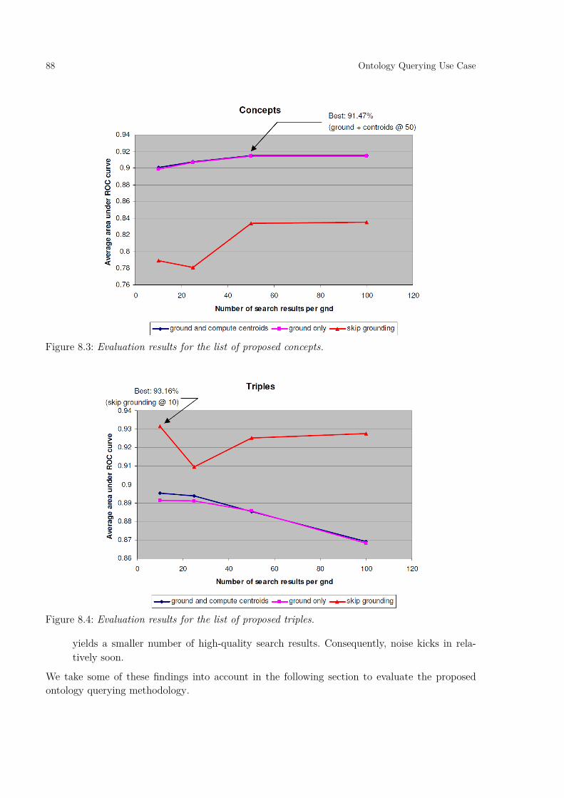
88 Ontology Querying Use Case
yields a smaller number of high-quality search results. Consequently, noise kicks in rela-tively soon.
We take some of these findings into account in the following section to evaluate the proposed ontology querying methodology.
Figure 8.3: Evaluation results for the list of proposed concepts.
Figure 8.4: Evaluation results for the list of proposed triples.

Ontology Querying Use Case 89
8.2.2 Graph-based algorithms
In this section, we evaluate the two graph-based algorithms discussed in Section 6.2.2: the Graph Of Concepts (GOC) and the Graph Of Triples (GOT). We show that these indeed significantly
Figure 8.5: Evaluation results for the list of proposed concepts.
Figure 8.6: Evaluation results for the list of proposed triples.
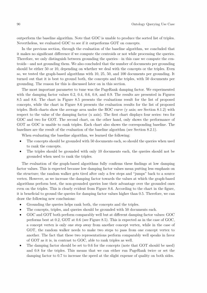
90 Ontology Querying Use Case
outperform the baseline algorithm. Note that GOC is unable to produce the sorted list of triples. Nevertheless, we evaluated GOC to see if it outperforms GOT on concepts.
In the previous section, through the evaluation of the baseline algorithm, we concluded that it makes no significant difference if we compute the centroids or not while processing the queries. Therefore, we only distinguish between grounding the queries—in this case we compute the cen-troids—and not grounding them. We also concluded that the number of documents per grounding should be either 50 or 10, depending on whether we deal with the concepts or the triples. Even so, we tested the graph-based algorithms with 10, 25, 50, and 100 documents per grounding. It turned out that it is best to ground both, the concepts and the triples, with 50 documents per grounding. The reason for this is discussed later on in this section.
The most important parameter to tune was the PageRank damping factor. We experimented with the damping factor values 0.2, 0.4, 0.6, 0.8, and 0.9. The results are presented in Figures 8.5 and 8.6. The chart in Figure 8.5 presents the evaluations result for the list of proposed concepts, while the chart in Figure 8.6 presents the evaluation results for the list of proposed triples. Both charts show the average area under the ROC curve (y axis; see Section 8.1.2) with respect to the value of the damping factor (x axis). The first chart displays four series: two for GOC and two for GOT. The second chart, on the other hand, only shows the performance of GOT as GOC is unable to rank triples. Each chart also shows the corresponding baseline. The baselines are the result of the evaluation of the baseline algorithm (see Section 8.2.1).
When evaluating the baseline algorithm, we learned the following: • The concepts should be grounded with 50 documents each, so should the queries when used
to rank the concepts. • The triples should be grounded with only 10 documents each, the queries should not be
grounded when used to rank the triples.
The evaluation of the graph-based algorithms fully confirms these findings at low damping factor values. This is expected because low damping factor values mean putting less emphasis on the structure; the random walker gets tired after only a few steps and “jumps” back to a source vertex. However, as we increase the damping factor towards the values at which the graph-based algorithms perform best, the non-grounded queries lose their advantage over the grounded ones even on the triples. This is clearly evident from Figure 8.6. According to the chart in the figure, it is beneficial to ground the queries for damping factor values higher than 0.5. Therefore, we can draw the following new conclusions:
• Grounding the queries helps rank both, the concepts and the triples. • The concepts, triples, and queries should be grounded with 50 documents each. • GOC and GOT both perform comparably well but at different damping factor values: GOC
performs best at 0.2, GOT at 0.6 (see Figure 8.5). This is expected as in the case of GOC, a concept vertex is only one step away from another concept vertex, while in the case of GOT, the random walker needs to make two steps to pass from one concept vertex to another. The fact that these two representations perform comparably well speaks in favor of GOT as it is, in contrast to GOC, able to rank triples as well.
• The damping factor should be set to 0.6 for the concepts (note that GOT should be used) and 0.8 for the triples. This means that we can either run PageRank twice or set the damping factor to 0.7 to increase the speed at the slight expense of quality on both sides.

Ontology Querying Use Case 91
The rewarding fact is that we managed to significantly beat the baselines. We have increased the average AUC for 5.48% on the concepts and for 3.18% on the triples (in absolute terms). This presents a relatively big difference. For example, if the correct triples were distributed amongst the top 597 of 4,362 suggestions with the baseline algorithm (see Section 8.1.2 on as-sessing the value of AUC), they will now be distributed amongst the top 319 suggestions (almost half less). This means, roughly speaking, that the graph-based algorithms are twice as good as the baseline algorithm. Also, we believe that the user will have to inspect far less than 319 items to find the required building blocks as he will be able to interact with the system (i.e., re-formulate queries). To support this claim, we computed the average AUC by taking, for each annotation, only the most successful annotator into account (i.e., the annotator that formulated the query yielding the highest AUC). The average AUC on the triples rose to 98.15%. This reduces the number of items that need to be inspected from 319 to 161 (of 4,362) which is already very useful for the user. Note also that there may be some “true negatives” at the top of this list as our golden standard is not complete (at the time the golden standard annotations were defined, the ontology was not yet expressive enough).
These findings were adopted to implement the semi-automatic annotation capabilities in Vis-ual OntoBridge (Grčar and Mladenić, 2009; Grčar et al., 2012).


93
9 Conclusions and Further Work
The main goal of this thesis was to develop and implement TEHmINe, a methodology for mining text-enriched heterogeneous information networks. With respect to this, we first set several re-quirements to narrow down the infinite space of all possible methodologies. We then explored a range of methods from text mining, link analysis, and heterogeneous information network mining to devise the building blocks of the envisioned methodology. We demonstrated the use of TEHmINe in two different real-life use cases, showing its versatility, efficiency, and usefulness. In this chapter, we reevaluate the methodology with respect to the requirements set forth in Section 3.2. Finally, we conclude the thesis by presenting several ideas for further work.
9.1 Review of the methodology with respect to the require-ments
In Section 3.2, we posed several requirements for a general-purpose TEHIN mining methodology. In this section, we reevaluate the methodology with respect to these requirements. Bimodality The methodology (and the corresponding toolkit) needs to enable us to exploit both
textual and structural aspect of a TEHIN. This is the first of the three major requirements. It is implemented in the core of our methodology as a data fusion step that projects both types of data into a common vector space. We demonstrate its usefulness in the two presented use cases. In both cases, the setting in which we exploit both types of data outperforms the setting based only on text mining.
Heterogeneity The methodology needs to provide facilities to handle different types of objects and different types of links (heterogeneity) that are forming a heterogeneous information net-work. This is the second of the three major requirements. It is implemented as a three-step process. First, a heterogeneous information network is decomposed into a set of (homogeneous) graphs. Each aspect of heterogeneity is then handled separately. In the second step, each graph is embedded into a vector space, resulting in a set of structural vectors for each object. In the final step, the structural vectors (potentially together with the BOW vectors), corresponding to the same object, are fused together into a single BOW-like vector. In this data fusion step, it is possible to apply a feature weighting scheme that determines which types of information to emphasize and which to suppress.
Applicability The methodology needs to be applicable to a wide range of data mining problems involving text corpora, (heterogeneous) information networks, or text-enriched (heterogeneous) information networks. This is the last of the three major requirements. We reinterpreted this requirement as the ability to employ standard machine learning principles and techniques (e.g., feature selection and weighting, clustering, classification, ranking, regression, etc.). This is also the most important requirement that implies basing the methodology on an existing toolset

94 Conclusions and Further Work
for data mining. With respect to this, we based our methodology on a text mining framework. The fact that in the end, we project a TEHIN into a BOW-like space, enables us to use the data analysis algorithms that are available in the selected text mining toolkit. Since we de-scribe objects with vectors (rather than kernels or similarity matrices), our methodology is extremely versatile. We can employ feature-based methods (e.g., naive Bayes, nearest centroid classifier, Latent Semantic Indexing (LSI), feature selection techniques (see, e.g., Brank et al., 2008), 𝑘𝑘-means clustering), similarity-based methods (e.g., 𝑘𝑘-NN), and kernel-based methods (e.g., SVM). With respect to this, we can say that our methodology is widely applicable.
Uniformity The purpose of the methodology is to join the two worlds, text mining and network analysis, in a seamless way. The same modeling (analysis) tools should be able to handle both textual and structural data from a TEHIN. The preprocessing part of our methodology consists of two separate pipelines: the pipeline for processing texts and the pipeline for processing structure. Both types of data (texts and structure) are in the end projected into a common BOW-like vector space in which knowledge discovery is performed by using standard machine learning algorithms. These same machine learning algorithms can also be employed in scenar-ios when there is only text or only structure available.
Maturity The methodology should employ well-established and well-developed building blocks from the fields of text mining and network analysis. The first pipeline in the preprocessing part of the methodology workflow consists of well-established text mining components. They are employed for transforming texts into BOW vectors. The second pipeline, on the other hand, is based on Personalized PageRank (PPR). We can undoubtingly say that this part is also well-established as it is used in numerous applications. Finally, both types of data (texts and structure) are projected into a common BOW-like vector space in which knowledge dis-covery is performed by using standard (well-developed and well-established) machine learning algorithms suited for working with BOW vectors, similarity matrices, or kernels (such as naive Bayes, 𝑘𝑘-nearest neighbor, 𝑘𝑘-means clustering, and support vector machine).
Modularity The methodology needs to be representable as a set of components arranged into a data mining workflow. The methodology was presented as a set of workflows already in Chap-ter 3. These workflows were further detailed and upgraded in Chapters 5 and 6. The purpose of this requirement was to provide the basis for the implementation of the methodology in a workflow-based data mining environment.
Efficiency The devised methodology needs to allow for a fairly efficient implementation. The main components in our methodology are the standard text preprocessing routine and PPR. The text preprocessing routine is extremely efficient. The most problematic part is holding statistics for n-grams in the TF-IDF computation process, especially if n is large. This, how-ever, can be solved with an apriori-like algorithm which does several passes over the corpus, discarding terms with insufficient support after each pass. See, for example, Grčar et al. (2010) for an assessment of text preprocessing efficiency. The PPR computations, on the other hand, are more computationally expensive. However, since PageRank is extremely popular and useful, there is a substantial body of work done on speeding PPR up. The special case where PPR is run from a single source vertex is often referred to as a random walk with restart (RWR) in the literature. RWR approaches normally perform the relevance computation on a limited neighborhood of the source vertex by either resorting to graph partitioning or by bounding

Conclusions and Further Work 95
random walks (Fujiwara et al., 2012; Tong et al., 2006). Furthermore, we devised an algorithm for an efficient structure-based centroid computation with PPR. This centroid-computation algorithm can be used in the classical nearest centroid classifier. In case of having 𝑟𝑟 classes and 𝑛𝑛 objects, 𝑛𝑛 ≫ 𝑟𝑟, this speeds up the process by factor 𝑛𝑛𝑟𝑟 by computing 𝑟𝑟 PPR vectors instead of 𝑛𝑛 PPR vectors in the training phase.
9.2 Summary of contributions This thesis addresses the problem of discovering knowledge in large text corpora enriched with relational data which implicitly or explicitly provides semantic relations between the texts. Such relational data can be described in the form of a heterogeneous information network, a generali-zation of the standard information network. We could also say that we address knowledge dis-covery scenarios in which heterogeneous information networks are enriched with texts. We call such networks text-enriched heterogeneous information networks or TEHINs for short. The main motivation behind this work comes from the fact that the current general-purpose text mining toolkits are unable to handle relational information in a common knowledge discovery setting. In this thesis, we address this situation and develop TEHmINe, a general-purpose methodology for mining TEHINs in a typical text mining framework.
The main hypothesis researched in the thesis is that structural data, often available in real-world scenarios, can be exploited to improve the performance of algorithms employed for solving text mining tasks such as text classification and ranking. We show that it is possible to devise a methodology that supports this hypothesis and at the same time (i) is applicable to a wide range of data analysis problems, (ii) is devised as an easy-to-understand data analysis workflow, (iii) employs well-established data analysis techniques, and (iii) can be applied to large corpora of text documents accompanied with relatively large heterogeneous information networks. We test this hypothesis in two real-world use cases. In the video lecture categorization use case, we employ the devised methodology to combine textual data and structure from a TEHIN formed out of the available data. We show that the TEHIN contains a lot of useful information and that by employing the devised methodology, we are able to significantly outperform the standard text mining approach. Furthermore, in the ontology querying use case, the general idea is to rank ontology entities with respect to a query. The baselines are set with a standard text mining approach and by combining textual data and structure, we can significantly improve the perfor-mance of the developed ranking system over these baselines.
The main contributions of this thesis can be summarized as follows: • We introduced the concept of a text-enriched heterogeneous information network (TEHIN). • We provided a general overview of the related work from the fields of text mining, link
analysis, data fusion, and heterogeneous information network mining. • We provided a conceptual workflow-based overview of the proposed methodology for mining
TEHINs. • We argued for projecting graphs into vector spaces by using Personalized PageRank (PPR). • We presented (and argue for) a technique for decomposing a heterogeneous information
network into a set of graphs. • We presented a simple technique for combining BOW vectors and (several sets of) PPR
vectors into combined BOW-like vectors.
96 Conclusions and Further Work
• We presented an extremely efficient way of computing graph-based centroids and developed PRNCC, a PageRank-based nearest centroid classifier that uses the developed technique to substantially speed up the training phase.
• We implemented the text preprocessing routine as a software library called LATINO (Link analysis and text mining toolbox).
• We provided the functionality of LATINO as a set of ClowdFlows components. • We developed an automatic categorization tool for video lectures hosted at VideoLec-
tures.net. • We developed an approach to drawing relatively large graphs by using our vector-space
embedding technique. • We developed an approach to representing ontologies as graphs. • We developed and evaluated an approach to ontology querying. • We implemented Visual OntoBridge, a software application for supporting the user in a
semantic annotation task.
9.3 Future work This thesis develops a complete methodology rather than thoroughly exploring its parts. It leaves some steps rather pragmatic or even underdeveloped. Such a step is most notably the presented data fusion procedure. There is room for improvements also in other parts of the pipeline. The following are some ideas for further work. Disconnected components in derived graphs In Chapter 7 (esp. Section 7.6), we exposed
an issue that any algorithm for propagating labels or authority through a graph will face when dealing with disconnected components: the labels from one component will fail to reach the other components. Our methodology suggests decomposing a heterogeneous information net-work into a set of simple, homogeneous graphs. Even if the original network does not have any disconnected components, the derived graphs do not necessarily inherit this property. In our lecture categorization use case, this is most evident in the same-author graph which ex-hibits over 2,500 disconnected components, 1,643 of which contain no labeled vertices. This makes the same-author information harder to exploit and also results in the poorest contribu-tion to the overall categorization performance. It is worth exploring this issue further in order to propose a technique for interlinking such disconnected components. Here, we briefly present several ideas:
• Connecting disconnected components with links from other derived graphs. This is the simplest approach in which sparser graphs would inherit some links from denser graphs obtained from the same heterogeneous network. In our lecture categorization use case, we could, for example, interlink the disconnected components in the same-author graph with specific links from the same-event and viewed-together graphs. It is of course not clear which links to inherit in this way. One heuristic would be to connect the two vertices with the maximal joint degree. There are also other possibilities and would need to be more systematically explored.
• Using link prediction techniques. Another way to deal with this problem would be to employ link prediction techniques to induce inter-component links that would serve as bridges in the PageRank computation process. Since we are interested in links between disconnected components, the approaches based on the number of common neighbors

Conclusions and Further Work 97
(Newman, 2001a) are not suitable for this task. We could however implement the idea based solely on the degrees of the two vertices (Barabasi et al., 2002; Newman, 2001b). Furthermore, we could take one of the approaches specifically tailored for heterogeneous networks (Davis et al., 2011; Yang et al., 2012). This means that we would be able to infer links in sparse graphs from other types of structural information. For example, we would be able to predict same-author links by examining the same-event and viewed-together graphs, looking for correlations between these different types of links.
• Using a less sparse derived graph to propagate sparse information. In our methodology, we suggest to run PPR from a vertex and in effect compute a feature vector describing how well the vertex is connected (similar, close) to each other vertex. This basically means that a vertex is described with other vertices. We could reformulate this step to instead describe a vertex with other vertices’ features. Imagine that we have two derived graphs, the same-author graph (extremely sparse; many disconnected components) and the viewed-together graph (much denser; one single component), both obtained from the same heterogeneous network. Instead of running PPR on the same-author graph in isolation, we could propagate the same-author information across the viewed-together graph. One way to efficiently do this would be to run PPR on the viewed-together graph and compute a linear combination of the author feature vectors, weights being the PPR scores. This and other possible approaches would need to be more thoroughly explored.
Weight optimization process in the data fusion step In the data fusion step of the pro-posed methodology, the idea is to assign a weight to each different type of data in an attempt to optimize the selected performance metric. This part of the methodology is clearly under-specified in this thesis. In the lecture categorization use case, we perform differential evolution which is a stochastic optimization technique. Another possibility would be to employ multiple kernel learning in a classification setting (as in Lanckriet et al. (2004)). The problem with a stochastic optimization loop is that it is fairly inefficient while the problem with MKL is that it restrains the knowledge discovery process mainly to kernel-based methods. The proposed methodology would be greatly improved if a general-purpose technique for optimizing the weights in a more efficient way would be devised. It would be possible to tune a weight ac-cording to how well the corresponding feature set performs in isolation or how sparse the corresponding graph is (these two aspects are actually highly correlated). By observing these initial weights, it would be possible to introduce various constraints into a stochastic optimi-zation process (e.g., the weight of the same-author feature set should be lower than the weight of the same-event feature set). It would also be possible to devise a (greedy) stepwise optimi-zation process, optimizing one single parameter in each step (i.e., α·feature-set1 + (1–α)·feature-set2). In general, there are many possibilities to tune the weights; they should be thoroughly explored and evaluated.
IDF-like component in vertex weights In the text preprocessing step, texts are converted into BOW vectors. BOW vectors are high-dimensional sparse vectors in which dimensions are defined by words and terms. A popular scheme for computing weights in such vectors is the so-called TF-IDF weighting scheme. This scheme weights a term higher if it occurs often in the same text (the TF component) and at the same time lower if it occurs in many texts from the corpus (the IDF component). In Section 5.2.2, we show an analogy between PPR and TF weights, arguing that we are able to project networks into BOW-like vector spaces. We, how-ever, disregard the IDF component which has a clear intuitive meaning in text mining and is
98 Conclusions and Further Work
usually shown to improve the results of a knowledge discovery process. It would be possible to transfer the intuition that common features are less important, into our structural feature vector computation process. Our preliminary experiments, not presented in this thesis, show that a simple heuristic, in which the PPR weight is multiplied by the logarithm of the total number of vertices divided by the degree of the corresponding vertex (which resembles the IDF formula), already outperforms the proposed weight computation process in the presented lecture categorization use case. This and other similar heuristics should be studied more thor-oughly.
Faster PPR computation Computing PPR is one of the key processes in our methodology. In general, several PPR vectors are computed for each vertex (one for each different type of structural information). It is thus crucial to compute PPRs as fast as possible. Since PageRank is relatively popular and generally useful, there is a substantial body of work done on speeding PPR up. The special case where PPR is run from a single source vertex is often referred to as a random walk with restart (RWR) in the literature. Tong et al. (2006) discuss several ap-proaches to fast approximate RWR computations by resorting to graph partitioning techniques. They perform RWR only on the sub-graph that contains the source vertex and set the rele-vance scores of the vertices outside this sub-graph to 0. In a different approach, Fujiwara et al. (2012) compute an upper relevance bound in order to avoid computing relevance scores for vertices that are too far from the source vertex. In this thesis, we use the original formulation (implementation) of PPR. We propose to study fast algorithms for approximate PPR compu-tation more thoroughly and assess their impact on the performance in knowledge discovery settings.
Implementation of ClowdFlows components The components, presented in this thesis, were initially implemented as two academic prototypes, employing the devised methodology (or parts of it) in the two presented use cases. The first prototype is the VideoLectures.net categorization tool which categorizes video lectures into a taxonomy of scientific topics. The second prototype is Visual OntoBridge, a system that employs the presented methodology for ontology querying. The text mining process as well as the PageRank computation routine, employed in these prototypes, is implemented as a software library called LATINO (Link analysis and text mining toolbox). Some of the functionality of LATINO is provided also as a set of ClowdFlows components for text preprocessing and machine learning. Several method-ology components, however, were not reimplemented as ready-to-use components or a software library. Such components are most notably the following: (i) graph extraction (a general-purpose component for creating graphs out of TEHINs), (ii) PPR (even though PPR is avail-able in LATINO, it is not available as a ClowdFlows component for embedding graphs into vector spaces), and (iii) data fusion (a general-purpose data fusion component as envisioned by the proposed methodology). In addition, two more components could be implemented: (i) PPR-based nearest centroid classifier (see Section 5.3.2) and (ii) graph visualization tool (see Section 7.6). We leave these implementation efforts for further work.

99
Acknowledgements
First of all, I would like to express my thanks to my supervisor Nada Lavrač for her support, guidance, help, and patience.
My thanks also go to the members of the committee, Ljupčo Todorovski, Janez Demšar, and Igor Mozetič, for their comments and suggestions which improved the quality of this thesis.
For the mentorship and support in the earlier days, I would like to express my sincere gratitude to Marko Grobelnik and Dunja Mladenić.
This work was (partly) funded by the European Commission through the research projects TAO, SWING, and ENVISION. Respectively, I would also like to thank all the consortia members with whom I have collaborated in these projects—it was a pleasure.
I would like to thank the VideoLectures.net team, esp. Peter Keše and everybody from the Center for Knowledge Transfer, for providing the data and domain knowledge for carrying out the VideoLectures.net categorization use case.
My warm thanks go to Matjaž Juršič who took my text mining framework to a new level by implementing a set of ClowdFlows widgets. This was a huge effort that resulted in over 100 interoperable components which went way beyond being just simple wrappers.
My thanks also go to Matic Perovšek who selflessly integrated the LATINO ClowdFlows widg-ets into his text mining platform TextFlows. This gesture was much more than just an engineering effort; it made LATINO publicly available in a user-friendly way and integrated it with other text mining toolkits, making it more relevant and “fashionable”.
I would like to thank everybody at the Department of Knowledge Technologies for contributing to a stimulating and friendly working environment. Special thanks to my office mates, present and past, for the countless discussions and uplifting spirit.
Last but certainly not least, my warmest thanks and love to my wife Tanja who supported me, and supports me still, for better or for worse, in my sometimes foolish pursuit of goals.

101
References
Andrei, M.; Berre, A.; Costa, L.; Duchesne, P.; Fitzner, D.; Grčar, M.; Hoffmann, J.; Klien, E.; Langlois, J.; Limyr, A.; Maue, P.; Schade, S.; Steinmetz, N.; Tertre, F.; Vasiliu, L.; Zaharia, R.; Zastavni, N. SWING: An Integrated Environment for Geospatial Semantic Web Services. In: Proceedings of the 6th European Semantic Web Conference (ESWC), Lecture Notes in Computer Science 5021, 767–771 (Springer, Berlin, Heidelberg, New York, 2008).
Atrey, P. K.; Hossain, M. A.; El, S. A.; Kankanhalli, M. S. Multimodal Fusion for Multimedia Analysis: A Survey. Multimedia Systems 16, 345–379 (2010).
Balmin, A.; Hristidis, V.; Papakonstantinou, Y. ObjectRank: Authority-based Keyword Search in Databases. In: Proceedings of the 30th International Conference on Very Large Databases. 564–575 (VLDB Endowment, USA, Toronto, Canada, 2004).
Barabasi, A.; Jeong, H. K.; Neda, Z.; Ravasz, E.; Schubert, A.; Vicsek, T. Evolution of the Social Network of Scientific Collaborations. Physica A: Statistical Mechanics and Its Applications 311, 590–614 (2002).
Bhagat, S.; Cormode, G.; Muthukrishnan, S. Node Classification in Social Networks. Social Net-work Data Analytics. 115–148 (2011).
Brank, J.; Mladenić, D.; Grobelnik, M.; Milić-Frayling, N. Feature Selection for the Classification of Large Document Collections. Journal of Universal Computer Science 14, 1562–1596 (2008).
Burt, R. S.; Minor, M. J. Applied Network Analysis: A Methodological Introduction (Sage Publi-cations, Newbury Park CA, 1983).
Cannon, R. L.; Dave, J. V.; Bezdek, J. C. Efficient Implementation of the Fuzzy c-Means Clus-tering Algorithms. IEEE Transactions on Pattern Analysis and Machine Intelligence 8, 248–255 (1986).
Cardoso-Cachopo, A.; Oliveira, A. L.; Redol, I. R. A. Empirical Evaluation of Centroid-based Models for Single-label Text Categorization, INSEC-ID Technical Report 7/2006 (Instituto Superior Técnico, DEI, Av. Rovisco Pais, 1, 1049-001 Lisboa, Portugal, 2006).
Caruana, R.; Munson, A.; Niculescu-Mizil, A. Getting the Most out of Ensemble Selection. In: Proceedings of the 6th International Conference on Data Mining (ICDM'06). 828–833 (IEEE Computer Society, USA, Hong Kong, China, 2006).
Cavnar, W. B.; Trenkle, J. M. N-Gram-Based Text Categorization. In: In Proceedings of SDAIR-94, 3rd Annual Symposium on Document Analysis and Information Retrieval. 161–175 (UNLV Publications, Las Vegas, USA, 1994).
Cestnik, B. Ocenjevanje verjetnosti v avtomatskem učenju, PhD Thesis (Faculty of Computer and Information Science, University of Ljubljana, Ljubljana, 1991).
102 References
Cover, T.; Hart, P. Nearest Neighbor Pattern Classification. IEEE Information Theory Society 13, 21–27 (2006).
Crammer, K.; Singer, Y. On the Algorithmic Implementation of Multiclass Kernel-based Vector Machines. Journal of Machine Learning Research 2, 265–292 (2002).
Crestani, F. Application of Spreading Activation Techniques in Information Retrieval. Artificial Intelligence Review 11, 453–482 (1997).
Cullum, J. K.; Willoughby, R. A. Lanczos Algorithms for Large Symmetric Eigenvalue Compu-tations, Vol. 1 (Society for Industrial and Applied Mathematics, Philadelphia, PA, USA, 2002).
Davis, D.; Lichtenwalter, R.; Chawla, N. V. Multi-relational Link Prediction in Heterogeneous Information Networks. In: Proceedings of the 2011 International Conference on Advances in Social Networks Analysis and Mining. 281–288 (IEEE Computer Society, Washington, DC, USA, 2011).
Dempster, A. P.; Laird, N. M.; Rubin, D. B. Maximum Likelihood from Incomplete Data via the EM Algorithm. Journal of the Royal Statistical Society, Series B 39, 1–38 (1977).
Džeroski, S.; Lavrač, N. Relational Data Mining (Springer-Verlag, Berlin, 2001).
Feldman, R.; Sanger, J. The Text Mining Handbook: Advanced Approaches in Analyzing Unstruc-tured Data (Cambridge University Press, Cambridge, England and New York, USA, 2006).
Fellbaum, C. WordNet: An Electronic Lexical Database (Bradford Books, Colorado, USA, 1998).
Fortuna, B.; Mladenić, D.; Grobelnik, M. Semi-Automatic Construction of Topic Ontology. In: Proceedings of the Conference on Data Mining and Data Warehouses (SiKDD 2005), Seman-tics, Web and Mining. 121-131 (Springer, Heidelberg, 2005).
Fortuna, B.; Mladenić, D.; Grobelnik, M. Visualization of Text Document Corpus. Informatica 29, 497–502 (2006).
Fu, G.; Luke, K. A Two-stage Statistical Word Segmentation System for Chinese. In: Proceedings of the Second Sighan Workshop on Chinese Language Processing 17, 156–159 (Association for Computational Linguistics, Stroudsburg, PA, USA, 2003).
Fujiwara, Y.; Nakatsuji, M.; Yamamuro, T.; Shiokawa, H.; Onizuka, M. Efficient Personalized Pagerank with Accuracy Assurance. In: Proceedings of the 18th ACM SIGKDD International Conference on Knowledge Discovery and Data Mining. 15–23 (ACM, New York, NY, USA, 2012).
Gärtner, T. A Survey of Kernels for Structured Data. SIGKDD Explorations 5, 49–58 (2003).
Getoor, L.; Diehl, C. P. Link Mining: A Survey. SIGKDD Explorations Special Issue on Link Mining 7, 3–12 (2005).
Goh, C.; Asahara, M.; Matsumoto, Y. Chinese Word Segmentation by Classification of Charac-ters. Computational Linguistics and Chinese Language Processing 10, 381–396 (2005).
References 103
Grčar, M.; Lavrač, N. A Methodology for Mining Document-Enriched Heterogeneous Information Networks. In: Proceedings of the 14th International Conference on Discovery Science, Lecture Notes in Computer Science Volume 6926, 107–121 (Springer, Berlin, Heidelberg, New York, 2011).
Grčar, M.; Mladenić, D. Visual OntoBridge: Semi-Automatic Semantic Annotation Software. In: Proceedings of the European Conference on Machine Learning and Principles and Practice of Knowledge Discovery in Databases (ECML-PKDD), Lecture Notes in Computer Science 5782, 726–729 (Springer, Berlin, Heidelberg, New York, 2009).
Grčar, M.; Mladenić, D.; Grobelnik, M. User Profiling for Interest-Focused Browsing History. In: Proceedings of the 8th Multiconference Information Society IS 2005. 182–185 (Jožef Stefan Institute, Ljubljana, 2005).
Grčar, M.; Mladenić, D.; Keše, P. Semi-Automatic Categorization of Videos on VideoLectures.net. In: Proceedings of the European Conference on Machine Learning and Principles and Practice of Knowledge Discovery in Databases (ECML-PKDD), Lecture Notes in Computer Science 5782, 730–733 (Springer, Berlin, Heidelberg, New York, 2009a).
Grčar, M.; Klien, E.; Novak, B. Using Term-Matching Algorithms for the Annotation of Geo-services. In: Knowledge Discovery Enhanced with Semantic and Social Information 220, 127–143 (Springer, Berlin, Heidelberg, New York, 2009b).
Grčar, M.; Podpečan, V.; Juršič, M.; Lavrač, N. Efficient Visualization of Document Streams. In: Proceedings of the 13th International Conference on Discovery Science, Lecture Notes in Com-puter Science 6332, 174–188 (Springer, Berlin, Heidelberg, New York, 2010).
Grčar, M.; Podpečan, V.; Sluban, B.; Mozetič, I. Ontology Querying Support in Semantic Anno-tation Process. In: Lecture Notes in Computer Science 7458, 76–87 (Springer, Berlin, Heidel-berg, New York, 2012).
Grčar, M.; Trdin, N.; Lavrač, N. A Methodology for Mining Document-Enriched Heterogeneous Information Networks. The Computer Journal 56, 321–335 (2013).
Grobelnik, M.; Mladenić, D. Simple Classification into Large Topic Ontology of Web Documents. Journal of Computing and Information Technology 13, 279–285 (2005).
Gruber, T. R. A Translation Approach to Portable Ontology Specifications. Knowledge Acquisi-tion 5, 199–220 (1993).
Han, E.; Karypis, G. Centroid-Based Document Classification: Analysis and Experimental Re-sults. In: Proceedings of the 4th European Conference on Principles of Data Mining and Knowledge Discovery. 424–431 (Springer-Verlag, London, UK, 2000).
Hassler, M.; Fliedl, G. Text Preparation through Extended Tokenization. In: Data Mining VII: Data, Text and Web Mining and Their Business Applications 37, 13–21 (WIT Press/Compu-tational Mechanics Publications, Southampton, UK, 2006).
Hsu, C.; Lin, C. A Comparison of Methods for Multiclass Support Vector Machines. IEEE Trans-actions on Neural Networks 13, 415–425 (2002).

104 References
Hwang, T.; Kuang, R. A Heterogeneous Label Propagation Algorithm for Disease Gene Discovery. In: Proceedings of the 10th SIAM International Conference on Data Mining, SDM. 583-594 (SIAM, Philadelphia, US, 2010).
Jeh, G.; Widom, J. SimRank: A Measure of Structural-context Similarity. In: Proceedings of the eighth ACM SIGKDD International Conference on Knowledge Discovery and Data Mining. 538-543 (ACM, New York, USA, Edmonton, Alberta, Canada, 2002).
Ji, M.; Sun, Y.; Danilevsky, M.; Han, J.; Gao, J. Graph Regularized Transductive Classification on Heterogeneous Information Networks. In: Proceedings of the 2010 European Conference on Machine Learning and Knowledge Discovery in Databases: Part I. 570–586 (Springer-Verlag, Berlin, Germany, Barcelona, Spain, 2010).
Ji, M.; Han, J.; Danilevsky, M. Ranking-based Classification of Heterogeneous Information Net-works. In: Proceedings of the 17th ACM SIGKDD International Conference on Knowledge Discovery and Data Mining. 1298–1306 (ACM, New York, NY, USA, 2011).
Joachims, T.; Finley, T.; Yu, C. J. Cutting-plane Training of Structural SVMs. Machine Learning 77, 27–59 (2009).
Joachims, T. Text Categorization with Support Vector Machines: Learning with Many Relevant Features. In: Proceedings of the 10th European Conference on Machine Learning. 137–142 (Springer-Verlag, London, UK, UK, 1998).
Joachims, T. Making Large-scale Support Vector Machine Learning Practical (MIT Press, Cam-bridge, MA, USA, 1999).
Joachims, T. Learning to Classify Text Using Support Vector Machines: Methods, Theory and Algorithms (Kluwer Academic Publishers, Norwell, MA, USA, 2002).
Juršič, M.; Mozetič, I.; Erjavec, T.; Lavrač, N. LemmaGen: Multilingual Lemmatisation with Induced Ripple-Down Rules. Journal of Universal Computer Science 16, 1190-1214 (2010).
Kim, H.; Chan, P. K. Learning Implicit User Interest Hierarchy for Context in Personalization. Applied Intelligence 28, 153–166 (2008).
Kleinberg, J. M. Authoritative Sources in a Hyperlinked Environment. Journal of the Association for Computer Machinery 46, 604–632 (1999).
Kondor, R. I.; Lafferty, J. Diffusion Kernels on Graphs and Other Discrete Structures. In: Pro-ceedings of the 19th International Conference on Machine Learning: ICML. 315–322 (Morgan Kaufmann, San Francisco, USA, Sydney, Australia, 2002).
Kramer, S.; Lavrač, N.; Flach, P. Propositionalization Approaches to Relational Data Mining (Springer, New York, USA, 2001).
Kranjc, J.; Podpečan, V.; Lavrač, N. ClowdFlows: A Cloud Based Scientific Workflow Platform (Springer, Heidelberg, Germany, 2012).
Krek, S. Pridobivanje jezikovnih podatkov iz besedilnih korpusov za namen izdelave enojezičnih slovarjev in slovnic, PhD Thesis (Faculty of Arts, University of Ljubljana, Ljubljana, Slovenia, 2010).
References 105
Lanckriet, G. R. G.; Deng, M.; Cristianini, N.; Jordan, M. I.; Noble, W. S. Kernel-Based Data Fusion and Its Application to Protein Function Prediction in Yeast. In: Proceedings of the Pacific Symposium on Biocomputing. 300–311 (World Scientific, New Jersey, USA, Hawaii, USA, 2004).
Lang, K. Fixing Two Weaknesses of the Spectral Method. Advances in Neural Information Pro-cessing Systems 18, 715–722 (2005).
Lavrač, N.; Džeroski, S. Inductive Logic Programming: Techniques and Applications (Ellis Hor-wood, UK, 1994).
Leskovec, J.; Grobelnik, M.; Milic-Frayling, N. Learning Semantic Graph Mapping for Document Summarization. In: Proceedings of the ECML/PKDD-2004 Workshop on Knowledge Discovery and Ontologies (KDO-2004). 1–6 (Pisa, Italy, 2004).
Ley, M. The DBLP Computer Science Bibliography: Evolution, Research Issues, Perspectives. In: String Processing and Information Retrieval 2476, 1–10 (Springer, Berlin, Heidelberg, New York, 2002).
Lloyd, S. Least Squares Quantization in PCM. IEEE Transactions on Information Theory 28, 129–137 (2006).
Lo, R. T.; He, B.; Ounis, I. Automatically Building a Stopword List for an Information Retrieval System. Journal of Digital Information Management 3, 3–8 (2005).
Lu, Q.; Getoor, L. Link-based Text Classification. In: Proceedings of the Workshop on Text-Mining and Link-Analysis at Eighteenth International Joint Conference on Artificial Intelli-gence. 496–503 (Morgan Kaufmann, San Francisco, USA, Acapulco, Mexico, 2003).
Luxburg, U. A Tutorial on Spectral Clustering. Statistics and Computing 17, 395–416 (2007).
Manning, C. D.; Raghavan, P.; Schütze, H. Introduction to Information Retrieval (Cambridge University Press, New York, NY, USA, 2008).
Martin, E.; Hans-peter, K.; Jörg, S.; Xiaowei, X. A Density-based Algorithm for Discovering Clusters in Large Spatial Databases with Noise. In: Proceedings of the Second International Conference on Knowledge Discovery and Data Mining (KDD-96). 226–231 (AAAI Press, Menlo Park, CA, 1996).
McCallum, A.; Nigam, K. A Comparison of Event Models for Naive Bayes Text Classification. In: Proceedings of the AAAI-98 Workshop on Learning for Text Categorization. 41–48 (AAAI Press, Menlo Park, CA, 1998).
Meila, M.; Shi, J. A Random Walks View of Spectral Segmentation. In: Proceedings of the 8th International Conference on Artificial Intelligence and Statistics. 177-182 (IEEE Computer Society Press, Washington, DC, USA, 2001).
Miller, G. A. WordNet: A Lexical Database for English. Communications of the ACM 38, 39–41 (1995).
Mitchell, T. M. Machine Learning (McGraw-Hill, New York, USA, 1997).
Mladenić, D. Machine Learning on Non-homogeneous, Distributed Text Data, PhD Thesis (Fac-ulty of Computer and Information Science, University of Ljubljana, Ljubljana, Slovenia, 1998).

106 References
Muggleton, S. H. Inductive Logic Programming (Academic Press Ltd., London, UK, 1992).
Nadler, B.; Lafon, S.; Coifman, R. R.; Kevrekidis, I. G. Diffusion Maps, Spectral Clustering and Eigenfunctions of Fokker-Planck Operators. Advances in Neural Information Processing Sys-tems 18, 955–962 (2005).
Neville, J. Iterative Classification: Applying Bayesian Classifiers in Relational Data, Technical Report TR-00-31 (University of Massachusetts, Amherst, MA, USA, 2000).
Newman, M. E. J. Clustering and Preferential Attachment in Growing Networks. Physical Review E 64, 025102-1–025102-4 (2001a).
Newman, M. E. J. The Structure of Scientific Collaboration Networks. Proceedings of the National Academy of Sciences of the United States of America 98, 404–409 (2001b).
Ng, A. Y.; Jordan, M. I.; Weiss, Y. On Spectral Clustering: Analysis and an Algorithm. Advances in Neural Information Processing Systems 14, 849–856 (2001).
Nooy, W. D.; Mrvar, A.; Batagelj, V. Exploratory Social Network Analysis with Pajek (Cambridge University Press, Cambridge, UK and New York, USA, 2005).
Page, L.; Brin, S.; Motwani, R.; Winograd, T. The PageRank Citation Ranking: Bringing Order to the Web, Technical Report 1999-66 (Stanford InfoLab, Stanford, USA, 1999).
Pelleg, D.; Moore, A. X-means: Extending K-means with Efficient Estimation of the Number of Clusters. In: Proceedings of the 17th International Conference on Machine Learning. 727–734 (Morgan Kaufmann, San Francisco, USA, 2000).
Porter, M. F. An Algorithm for Suffix Stripping. Program 14, 130–137 (1980).
Rakesh, A.; Ramakrishnan, S. Fast Algorithms for Mining Association Rules. In: Proceedings of 20th International Conference on Very Large Data Bases. 487–499 (Morgan Kaufmann Pub-lishers Inc, San Francisco, CA, USA, 1994).
Rakotomamonjy, A.; Bach, F. R.; Canu, S.; Grandvalet, Y. SimpleMKL. Journal of Machine Learning Research 9, 2491–2521 (2008).
Salton, G.; McGill, M. J. Introduction to Modern Information Retrieval (McGraw-Hill, Inc., New York, NY, USA, 1986).
Salton, G. Automatic Text Processing: the Transformation, Analysis, and Retrieval of Information by Computer (Addison-Wesley Longman Publishing Co., Inc., Boston, USA, 1989).
Schmid, H. Tokenizing and Part-of-speech Tagging. In: Corpus Linguistics. An International Handbook. Handbooks of Linguistics and Communication Science 1, 527–551 (Mouton de Gruyter, Berlin, 2008).
Sclano, F.; Velardi, P. TermExtractor: A Web Application to Learn the Shared Terminology of Emergent Web Communities. In: Proceedings of I-ESA 2007. 287–290 (Springer London, Lon-don, UK, 2007).
Sebastiani, F. Machine Learning in Automated Text Categorization. ACM Computing Surveys 34, 1–47 (2002).

References 107
Shearer, C. The CRISP-DM Model: The New Blueprint for Data Mining. Journal of Data Ware-housing 5, 13–22 (2000).
Shi, J.; Malik, J. Normalized Cuts and Image Segmentation. IEEE Transactions on Pattern Analysis and Machine Intelligence 22, 888–905 (2000).
Silla, C. N. J.; Kaestner, C. A. A. An Analysis of Sentence Boundary Detection Systems for English and Portuguese Documents. In: Proceedings of the 5th International Conference on Computational Linguistics and Intelligent Text Processing, CICLing 2004. 135–141 (Springer, Berlin Heidelberg, 2004).
Singhal, A. Modern Information Retrieval: A Brief Overview. Bulletin of the IEEE Computer Society Technical Committee on Data Engineering 24, 35–42 (2001).
Sorkine, O.; Cohen-Or, D. Least-Squares Meshes. In: Proceedings of the Shape Modeling Interna-tional 2004. 191–199 (IEEE Computer Society, Washington, USA, Genova, Italy, 2004).
Steen, M. V. Graph Theory and Complex Networks: An Introduction (Maarten van Steen, Lex-ington, 2010).
Storn, R.; Price, K. Differential Evolution: A Simple and Efficient Heuristic for Global Optimi-zation over Continuous Spaces. Journal of Global Optimization 11, 341–359 (1997).
Stoyanovich, J.; Bedathur, S.; Berberich, K.; Weikum, G. EntityAuthority: Semantically Enriched Graph-Based Authority Propagation. In: Proceedings of 10th International Workshop on the Web and Databases (WebDB 2007). 1–10 (ACM, New York, USA, Beijing, China, 2007).
Sun, Y.; Han, J. Mining Heterogeneous Information Networks: Principles and Methodologies (Morgan & Claypool Publishers, CA, USA, 2012).
Sun, Y.; Han, J.; Zhao, P.; Yin, Z.; Cheng, H.; Wu, T. RankClus: Integrating Clustering with Ranking for Heterogeneous Information Network Analysis. In: Proceedings of the 12th Inter-national Conference on Extending Database Technology: Advances in Database Technology. 565-576 (ACM, New York, NY, USA, 2009a).
Sun, Y.; Yu, Y.; Han, J. Ranking-based Clustering of Heterogeneous Information Networks with Star Network Schema. In: Proceedings of the 15th ACM SIGKDD International Conference on Knowledge Discovery and Data Mining. 797-806 (ACM, New York, NY, USA, 2009b).
Tong, H.; Faloutsos, C.; Pan, J. Fast Random Walk with Restart and Its Applications. In: Pro-ceedings of the Sixth International Conference on Data Mining. 613–622 (IEEE Computer Society, Washington, DC, USA, 2006).
Tsochantaridis, I.; Hofmann, T.; Joachims, T.; Altun, Y. Support Vector Machine Learning for Interdependent and Structured Output Spaces. In: Proceedings of the Twenty-first Interna-tional Conference on Machine Learning. 104–111 (ACM, New York, NY, USA, 2004).
Vapnik, V. N. The Nature of Statistical Learning Theory (Springer-Verlag New York, Inc., New York, NY, USA, 1995).
Vieira, P. F.; Nonato, L. G.; Minghim, R. Visual Mapping of Text Collections through a Fast High Precision Projection Technique. In: Proceedings of the conference on Information Visu-alization. 282–290 (IEEE Computer Society, Washington, USA, Baltimore, USA, 2006).

108 References
Vishwanathan, S. V. N.; Sun, Z.; Ampornpunt, N.; Varma, M. Multiple Kernel Learning and the SMO Algorithm. Advances in Neural Information Processing Systems 23, 2361–2369 (2010).
Witten, I. H.; Frank, E.; Hall, M. A. Data Mining: Practical Machine Learning Tools and Tech-niques (Morgan Kaufmann, Amsterdam, 2011).
Xue, N.; Shen, L. Chinese Word Segmentation as LMR Tagging. In: Proceedings of the 2nd SIGHAN Workshop on Chinese Language Processing. 176–179 (Association for Computational Linguistics, Stroudsburg, PA, USA, 2003).
Yang, Y.; Nitesh, V. C.; Yizhou, S.; Jiawei, H. Predicting Links in Multi-relational and Hetero-geneous Networks. In: Proceedings of the 12th IEEE International Conference on Data Mining, ICDM 2012. 755–764 (IEEE Computer Society, Washington, DC, USA, 2012).
Zaman, A. N. K.; Matsakis, P.; Brown, C. Evaluation of Stop Word Lists in Text Retrieval Using Latent Semantic Indexing. In: Proceedings of the Sixth International Conference on Digital Information Management, ICDIM 2011. 133–136 (IEEE Press, Piscataway, NJ, USA, 2011).
Zhou, D.; Schölkopf, B. A Regularization Framework for Learning from Graph Data. In: Proceed-ings of the ICML Workshop on Statistical Relational Learning. 132–137 (ACM, New York, USA, Banff, Alberta, Canada, 2004).
Zhou, D.; Bousquet, O.; Lal, T. N.; Weston, J.; Schölkopf, B. Learning with Local and Global Consistency. Advances in Neural Information Processing Systems 16, 321–328 (2003).

109
Online references
[1] Web Service Modeling Language (WSML): http://www.w3.org/Submission/WSML [2] Wikipedia: Markov Chain: http://en.wikipedia.org/wiki/Markov_chain [3] Unicode Line Breaking Algorithm: http://www.unicode.org/reports/tr14 [4] SharpNLP Project: http://sharpnlp.codeplex.com [5] Snowball Project: http://snowball.tartarus.org [6] Lucene.Net Project: http://lucenenet.apache.org [7] LemmaGen Project: http://lemmatise.ijs.si [8] SVMlight Project: http://svmlight.joachims.org [9] SVMmulticlass Software:
http://www.cs.cornell.edu/People/tj/svm%5Flight/svm_multiclass.html [10] Yahoo! Directory: http://dir.yahoo.com [11] Open Directory (DMOZ): http://www.dmoz.org [12] Web Feature Service: http://www.opengeospatial.org/standards/wfs [13] Faroo Search Engine: http://www.faroo.com [14] Faroo Search API: http://www.faroo.com/hp/api/api.html [15] VideoLectures.net: http://videolectures.net [16] VideoLectures.net, TAO: Transitioning Applications to Ontologies:
http://videolectures.net/tao08_bled/ [17] Visual OntoBridge source code repository: http://source.ijs.si/mgrcar/visualontobridge [18] Visual OntoBridge Windows executable:
https://drive.google.com/file/d/0ByuNwpcPWf8gVGYwX3RWY3NFWmM/view [19] LATINO source code repository: http://source.ijs.si/mgrcar/latino [20] LATINO ClowdFlows components source code repository:
http://source.ijs.si/kt/textflows-net-sp [21] TextFlows source code repository: http://source.ijs.si/kt/textflows [22] TextFlows running instance: http://textflows.ijs.si [23] VideoLectures.net categorizer source code:
http://source.ijs.si/mgrcar/videolecturescategorizer [24] VideoLectures.net categorizer Windows executable:
https://drive.google.com/file/d/0ByuNwpcPWf8gbzhIVXNyaHZVeVU/view [25] Author’s bibliography in COBISS:
http://splet02.izum.si/cobiss/bibliography?code=28806&langbib=eng


111
Figures
Figure 2.1: Cross-Industry Standard for Data Mining (CRISP-DM)......................................... 10
Figure 3.1: Toy heterogeneous information network of conference papers. ................................. 16
Figure 3.2: Annotation as a ‘bridge’ between a resource and the domain ontology. ................... 18
Figure 3.3: A workflow-based overview of the TEHmINe methodology. ..................................... 19
Figure 3.4: A workflow-based overview of the proposed ontology querying methodology. ............ 21
Figure 4.1: A typical text preprocessing workflow (pipeline). ..................................................... 24
Figure 4.2: The cosine similarity measure. ................................................................................ 28
Figure 4.3: A prototypical ClowdFlows component. ................................................................... 36
Figure 4.4: An annotated document represented as HTML. ....................................................... 37
Figure 4.5: LATINO text preprocessing workflow (building a new BOW space). ....................... 37
Figure 4.6: LATINO text preprocessing workflow (projecting texts into an existing BOW space). .............................................................................................................................. 38
Figure 4.7: LATINO classification workflow (both the training and classification phase). ......... 38
Figure 4.8: LATINO clustering workflow. .................................................................................. 39
Figure 5.1: Dot product in a PPR space: the meeting probability. ............................................. 54
Figure 5.2: Cosine similarity in a PPR space: the random writer analogy. ............................... 55
Figure 5.3: Decomposition of the toy example from Section 3.1.1. ............................................ 56
Figure 5.4: Transforming a heterogeneous information network and the corresponding text documents into a joint feature vector format. .................................................................. 57
Figure 5.5: Proposed ClowdFlows workflow for embedding text-enriched heterogeneous information networks into vector spaces. ......................................................................... 60
Figure 6.1: Different approaches to processing user queries. ...................................................... 67
Figure 6.2: The process of constructing a graph of concepts from a TEHIN representing an ontology. ........................................................................................................................... 69
Figure 6.3: The process of constructing a graph of concepts (left) compared to the process of constructing a graph of triples (right). ......................................................................... 70
Figure 7.1: Visualization of the same-author vector space with the edges adopted from the corresponding graph. ......................................................................................................... 80
Figure 7.2: Visualization of the same-event vector space with the edges adopted from the corresponding graph. ......................................................................................................... 81
Figure 7.3: Visualization of the viewed-together vector space with the edges adopted from the corresponding graph. ................................................................................................... 82
112 Figures
Figure 7.4: The number of disconnected components and the number of components containing a certain number of categorized lectures for the same-author graph. .............. 83
Figure 7.5: The number of disconnected components and the number of components containing a certain number of categorized lectures for the same-event graph. ................ 83
Figure 8.1: The gold-standard acquisition form for the feature type “regions”. .......................... 86
Figure 8.2: Basic properties of the ROC curve. ......................................................................... 86
Figure 8.3: Evaluation results for the list of proposed concepts. ................................................. 88
Figure 8.4: Evaluation results for the list of proposed triples. .................................................... 88
Figure 8.5: Evaluation results for the list of proposed concepts. ................................................. 89
Figure 8.6: Evaluation results for the list of proposed triples. .................................................... 89
113
Tables
Table 7.1: The performance of the nearest centroid classifier for text categorization by using different BOW construction settings. ............................................................................... 75
Table 7.2: The results of the selected text classification algorithms and diffusion kernels. ......... 76
Table 7.3: The results of employing the proposed methodology. ................................................. 77
Table 7.4: The weights computed in the optimization process in Experiment 11. ....................... 77
Table 7.5: The weights computed in the optimization process in Experiment 12. ....................... 78
Table 7.6: The time, in seconds, spent for feature vector or kernel computation, training, and prediction. ................................................................................................................. 80
Table 8.1: Entities from the domain ontology. ........................................................................... 85

115
Author’s Bibliography
Publications related to this thesis
Journal paper Grčar, M.; Trdin, N.; Lavrač, N. A Methodology for Mining Document-Enriched Heterogeneous
Information Networks. The Computer Journal 56(3), 321–335, SCI IF 0.888 (2013).
Conference papers Grčar, M.; Lavrač, N. A Methodology for Mining Document-Enriched Heterogeneous Information
Networks. In: Proceedings of the 14th International Conference on Discovery Science, Lecture Notes in Computer Science 6926, 107–121 (Springer, Berlin, Heidelberg, New York, 2011).
Grčar, M.; Podpečan, V.; Juršič, M.; Lavrač, N. Efficient Visualization of Document Streams. In: Proceedings of the 13th International Conference on Discovery Science, Lecture Notes in Com-puter Science 6332, 174–188 (Springer, Berlin, Heidelberg, New York, 2010).
Grčar, M.; Mladenić, D.; Keše, P. Semi-Automatic Categorization of Videos on VideoLectures.net. In: Proceedings of the European Conference on Machine Learning and Principles and Practice of Knowledge Discovery in Databases (ECML-PKDD), Lecture Notes in Computer Science 5782, 726–729 (Springer, Berlin, Heidelberg, New York, 2009).
Grčar, M.; Podpečan, V.; Sluban, B.; Mozetič, I. Ontology Querying Support in Semantic Anno-tation Process. In: Proceedings of the 12th Pacific Rim International Conference on Artificial Intelligence (PRICAI), Lecture Notes in Computer Science 7458, 76–87 (Springer, Berlin, Heidelberg, New York, 2012a).
Andrei, M.; Berre, A.; Costa, L.; Duchesne, P.; Fitzner, D.; Grčar, M.; Hoffmann, J.; Klien, E.; Langlois, J.; Limyr, A.; Maue, P.; Schade, S.; Steinmetz, N.; Tertre, F.; Vasiliu, L.; Zaharia, R.; N, Z. SWING: An Integrated Environment for Geospatial Semantic Web Services. In: Proceedings of the 6th European Semantic Web Conference (ESWC), Lecture Notes in Com-puter Science 5021, 767–771 (Springer, Berlin, Heidelberg, New York, 2008).
Grčar, M.; Mladenić, D. Visual OntoBridge: Semi-Automatic Semantic Annotation Software. In: Proceedings of the European Conference on Machine Learning and Principles and Practice of Knowledge Discovery in Databases (ECML-PKDD), Lecture Notes in Computer Science 5782, 726–729 (Springer, Berlin, Heidelberg, New York, 2009).

116 Author’s Bibliography
Book chapters Grčar, M.; Klien, E.; Novak, B. Using Term-Matching Algorithms for the Annotation of Geo-
services. In: Berendt, B. et al. (eds) Knowledge Discovery Enhanced with Semantic and Social Information, Studies in Computational Intelligence 220, 127–143 (Springer, Berlin, Heidelberg, New York, 2009b).
Other publications and scientific contributions
A more complete list of author’s publications and contributions is available in COBISS (Online reference [25]).

117
Biography
Miha Grčar was born on March 2, 1979, in Kranj, Slovenia. He wrote his first computer program at the age of seven (in Basic on Commodore C64). While still in high school, Miha participated in the International Olympiads in Informatics (IOI): first in 1996 (in Portugal) and then in 1998 (in Hungary). He was also awarded several summer internships in Silicon Valley, at Hewlett-Packard Labs in Palo Alto, and at Hewlett-Packard in Cupertino. During these internships, Miha worked on an animation script interpreter, imaging libraries, and image formats. In 2005, he also spent several months at Microsoft Research in Cambridge, developing text mining tools for .NET.
Miha later started collaborating with Hewlett-Packard, initially through Hermes SoftLab. He later founded a startup company called While True in which he acted as the CEO. The company collaborated with Hewlett-Packard on several projects, most notably developing an implementa-tion of SVG (Scalable Vector Graphics). Miha left the company in 2004 to finish his studies and broaden his data mining know-how.
Miha studied computer science at the Faculty of Computer and Information Science (Univer-sity of Ljubljana) and obtained his bachelor’s degree in October 2006. His bachelor’s thesis stud-ied eccentricity of users in recommender systems. After graduating, Miha enrolled in a PhD program at the Jožef Stefan International Postgraduate School. His PhD thesis proposed a meth-odology for mining text-enriched heterogeneous information networks. The main challenge was to effectively and efficiently handle two types of data, texts and heterogeneous information net-works, in a common knowledge discovery framework.
After leaving While True, Miha got employed at Jožef Stefan Institute where he participated in numerous European projects. At the beginning, he was a member of the SEKT consortium (Semantically Enabled Knowledge Technologies; 2004–2006), later on he was a leader of work-packages in two STREP projects, TAO (Transitioning Applications to Ontologies; 2006–2008) and SWING (Semantic Web Services Interoperability for Geospatial Decision Making; 2006–2008).
In 2010, Miha acted as one of the initiators and principal researchers in the EU project FIRST (Large-Scale Information Extraction and Integration Infrastructure for Supporting Financial De-cision Making; 2011–2013). FIRST was committed to provide an infrastructure for analyzing vast streams of user-generated web content and news feeds from the domain of financial markets in near-real time. The developed technology was demonstrated in three use cases related to retail brokerage, reputation risk, and fraud detection.
In 2014, Miha joined Celtra, a global player in mobile ad creation, serving, and analytics. At Celtra, Miha worked on optimizing ad trafficking (Dynamic Creative Optimization; DCO) and on detecting anomalies in the trafficking/tracking data. In these projects, Miha employed opti-mization techniques (multi-armed bandit optimization), statistics, and machine learning.