text-based industry momentum...industry peers can explain these large industry momentum profits. we...
TRANSCRIPT

JOURNAL OF FINANCIAL AND QUANTITATIVE ANALYSIS Vol. 53, No. 6, Dec. 2018, pp. 2355–2388COPYRIGHT 2018, MICHAEL G. FOSTER SCHOOL OF BUSINESS, UNIVERSITY OF WASHINGTON, SEATTLE, WA 98195doi:10.1017/S0022109018000479
Text-Based Industry Momentum
Gerard Hoberg and Gordon M. Phillips*
AbstractWe test the hypothesis that low-visibility shocks to text-based network industry peers canexplain industry momentum. We consider industry peer firms identified through 10-K prod-uct text and focus on economic peer links that do not share common Standard IndustrialClassification (SIC) codes. Shocks to less visible peers generate economically large mo-mentum profits and are stronger than own-firm momentum variables. More visible tradi-tional SIC-based peers generate only small, short-lived momentum profits. Our findingsare consistent with momentum profits arising partially from inattention to economic linksof less visible industry peers.
I. IntroductionSince Jegadeesh and Titman (1993) reported the momentum anomaly, a large
literature has documented the magnitude of momentum, its pervasiveness in manysettings,1 and its potential explanations. Jegadeesh and Titman (2001), (2011) doc-ument the continued robustness of momentum in more recent years. Yet schol-ars continue to disagree about the causes of momentum. In their recent review,(Jegadeesh and Titman (2011), p. 507) state that “financial economists are farfrom reaching a consensus on what generates momentum profits, making this aninteresting area for future research.” We focus on the importance of horizontalindustry links between firms with varying degrees of visibility to investors andmomentum.
*Hoberg, [email protected], University of Southern California Marshall School of Busi-ness; Phillips (corresponding author), [email protected], Dartmouth CollegeTuck School of Business and National Bureau of Economic Research. We thank Jennifer Conrad(the editor), Michael Cooper, Kewei Hou (the referee), Dongmei Li, Peter MacKay, Oguz Ozbas,Jiaping Qiu, Merih Sevilir, Albert Sheen, Denis Sosyura, and seminar participants at the 2014Conference on Financial Economics and Accounting, Duisenberg School of Finance and Tinber-gen Institute, Erasmus University, Hebrew University, Interdisciplinary Center of Herzliya, McMasterUniversity, Rotterdam School of Management, Stanford University, Tel Aviv University, Tilberg Uni-versity, University of Chicago, University of Illinois, the University of Mannheim, the University ofMiami, and the University of Utah for helpful comments. All errors are the authors’ alone.
1Rouwenhorst (1998), (1999) further shows that momentum exists around the world, and Geb-hardt, Hvidkjaer, and Swaminathan (2005) show that it spills over into bond markets.
2355
https://doi.org/10.1017/S0022109018000479D
ownloaded from
https://ww
w.cam
bridge.org/core . IP address: 54.39.106.173 , on 22 Jul 2020 at 23:01:42 , subject to the Cambridge Core term
s of use, available at https://ww
w.cam
bridge.org/core/terms .

2356 Journal of Financial and Quantitative Analysis
Using the text-based network industry classification (TNIC) (Hoberg andPhillips (2016)) to identify peer firms, our first central finding is that industrymomentum profits are highly robust and substantially larger than previously doc-umented. Industry momentum was first documented by Moskowitz and Grinblatt(1999). However, Moskowitz and Grinblatt’s conclusion that industry momentummatters is called into question by Grundy and Martin (2001), who show that in-dustry momentum using peers based on Standard Industrial Classification (SIC)codes is not robust to the bid–ask bounce and to lagging the portfolio formationperiod by 1 month. We document that industry momentum is substantially moreimportant for less visible text-based industry peer firms, and this stronger form ofindustry momentum is highly robust to the issues raised by the Grundy and Martincritique.
Recently, Hong and Stein (1999) and Barberis, Shleifer, and Vishny (1998)suggest that inattention or slow-moving information might also be a key driver ofmomentum. Our second central finding is that inattention to shocks to less visibleindustry peers can explain these large industry momentum profits.
We note 5 key results that support our conclusion that inattention is likely acentral explanation for the industry momentum we document. First, the economicmagnitudes are too large to be explained by simple differences in the informationcontent of industry classifications. For example, Hoberg and Phillips (2016) findthat TNIC is roughly 25% to 40% more informative than SIC codes in their abilityto explain a battery of variables in cross section. These gains are much smallerthan the 100% to 200% improvements in momentum profits we document here.
Second, we find that industry momentum profits are stronger followingshocks to specific peers that are less visible to the investment community. SICpeers are widely reported in financial databases, financial reports, regulatory dis-closures, and online data resources. However, TNIC peer data were not widelydistributed during our sample period, and the first paper focusing on TNIC peers(Hoberg and Phillips (2010)) was published late in our sample period.2 BecauseTNIC and SIC both capture horizontal relatedness, we consider TNIC peers thatare not SIC peers to examine the role of visibility. We predict and find that shocksto TNIC peers that are not SIC peers, and shocks in product markets whereSIC and TNIC peers disagree (high disparity), generate the strongest momentumreturns.
Third, we find that the timing of momentum profits due to shocks to SICpeer firms versus less visible TNIC peer firms is fundamentally different. Stockreturn shocks to SIC peers transmit to the focal firm in 1 to 2 months. In contrast,and consistent with inattention and slow-moving information, analogous shocksto less visible TNIC peers take up to 12 months to transmit. We also find thatown-firm share turnover increases only with significant lags when TNIC peershave high stock returns, whereas share turnover increases immediately when SICpeers are similarly shocked.
2Publication dates of academic articles pertaining to predictable stock returns are relevant, asMcLean and Pontiff (2016) find evidence that anomalies attenuate after such publication, perhapsbecause of increased attention.
https://doi.org/10.1017/S0022109018000479D
ownloaded from
https://ww
w.cam
bridge.org/core . IP address: 54.39.106.173 , on 22 Jul 2020 at 23:01:42 , subject to the Cambridge Core term
s of use, available at https://ww
w.cam
bridge.org/core/terms .

Hoberg and Phillips 2357
Under the inattention hypothesis, a related prediction is that systematicshocks, which are highly visible by definition, will decay more quickly thanidiosyncratic shocks, which are localized and less visible. Alternative risk-basedtheories predict that returns will be linked more to systematic shocks than toidiosyncratic shocks. We find that only idiosyncratic shocks transmit slowly andgenerate industry momentum. These findings are consistent with inattention andnot systematic risk-based explanations.
Fourth, in a direct test of inattention to economic links motivated by Cohenand Frazzini (2008), we find that longer term industry momentum profits existonly when mutual funds on average do not jointly own economically linked firms.This implies profits are largest where there is little institutional attention to thegiven economic links. Our results suggest that momentum is stronger when fewerprofessional investors (mutual fund managers) are paying attention to our lessvisible economically linked firms, as they are not in the portfolios of professionalinvestors. Supporting the conclusion that information about TNIC-related firms isless visible to the market, we find that sector funds are more likely to own pairs offirms that are in the same SIC code but are less likely to own pairs of TNIC peerfirms.
Fifth, we find that momentum profits are driven by economic links that arerelatively local in the product market network. The spatial nature of TNIC indus-tries allows us to examine whether momentum is related to the breadth of variouspeer shocks. We define broad shocks as those that affect a large set of relatedfirms that are distant in the product market space, whereas localized shocks affectonly a small number of proximate firms. We find that local TNIC peers calibratedto be as fine as the SIC 4-digit (SIC-4) classification generate strong momen-tum returns, as do TNIC peers that are calibrated to be as fine as the SIC 3-digit(SIC-3) network. We also find and report that broader TNIC peers, calibrated tobe as coarse as the SIC 2-digit (SIC-2) industry network, still generate significantindustry momentum profits, albeit at a lower magnitude. Our results suggest thatonly 2% to 5% of all firm pairs are needed to explain industry momentum, con-sistent with momentum being idiosyncratic and localized in the product market.
Our results thus support the following interpretation of momentum profitcycles. Initially, the market underreacts to large shocks to economically linkedfirms. This underreaction is more severe when the economic links are less visible.Furthermore, the time required for shocks to transmit is substantially longer.
Our findings indicate that industry momentum profits have high Sharperatios, as they can be easily diversified despite their high returns. These findingscannot be explained by a systematic risk explanation and overall are consistentwith inattention driving at least part of industry momentum profits.3
3Systematic risk models, which require transparency for equilibrium pricing, predict that linkswith more visibility should generate stronger risk premia. Investors need to be aware of risk loadingsto price them in equilibrium. Risk models also require that systematic shocks are pervasive and difficultto diversify. In conflict with these predictions, we instead find that less visible links matter more thanhighly visible links, and we find that momentum is most priced when shocks are localized, unrelatedto risk factors, and thus easier to diversify. Griffin, Ji, and Martin (2003) also suggest that systematicrisk likely cannot explain momentum through a different test (the absence of a business-cycle effect).
https://doi.org/10.1017/S0022109018000479D
ownloaded from
https://ww
w.cam
bridge.org/core . IP address: 54.39.106.173 , on 22 Jul 2020 at 23:01:42 , subject to the Cambridge Core term
s of use, available at https://ww
w.cam
bridge.org/core/terms .

2358 Journal of Financial and Quantitative Analysis
We examine various momentum horizon variables to further assess thefindings of Jegadeesh and Titman (1993) and Moskowitz and Grinblatt (1999).Using the standard 1-year momentum horizon, we find that the less visibleTNIC peer momentum variables are substantially more significant than are SICpeers or own-firm momentum variables in standard Fama–MacBeth (1973) returnregressions. Moreover, the economic magnitude of TNIC peer momentum vari-ables is considerably larger. Our results are strong for both the 6-month horizonand the subsequent 6-month period from months t+7 to t+12.
Our findings run counter to recent conclusions on industry momentum inthe literature, as Grundy and Martin (2001) show that industry momentum forSIC peers is not robust to the bid–ask bounce and to lagging the portfolio forma-tion period by 1 month. To underscore this point, Jegadeesh and Titman (2011)highlight Grundy and Martin’s findings in their review and conclude that industrymomentum cannot explain the momentum anomaly. However, they do concludethat momentum profits likely “arise because of a delayed reaction to firm-specificinformation” (Jegadeesh and Titman (2011), p. 497). The conclusion in the liter-ature that industry momentum matters little is thus based on using highly visibletraditional SIC-based industry links. We show that this long–standing conclusionis reversed when less visible text-based industry links are used to retest the indus-try momentum hypothesis.
Recent work by Cohen and Frazzini (2008) and Menzley and Ozbas (2010)suggests that inattention also plays a role in generating predictable returns follow-ing shocks to vertically linked firms. We focus on shocks to horizontally linkedfirms and not to vertically linked firms, and our objective is to address the industrymomentum literature. Controls for shocks to vertically linked firms do not mate-rially affect our results. Furthermore, only shocks to our less visible horizontalindustry peers, and not vertical peers, can explain own-firm momentum. The find-ing that vertical and horizontal peers contain distinct information is expected ashorizontal economic links overlap little with vertical links, as reported in Hobergand Phillips (2016).
Our results are consistent with the momentum literature in terms of the dura-tion of momentum profits being roughly 12 months. These long horizons explainwhy our results are not driven by the existing short-horizon finding that largefirm returns lead small firm returns especially within industry (see Hou (2007)).Moreover, our results are robust to controlling for lagged return variables used inHou (2007), including lagged return variables based on larger firms.
This article is organized as follows: Section II presents hypotheses motivatedby the theoretical models of Hong and Stein (1999) and Barberis et al. (1998).Section III describes our data and methods. Section IV presents initial evidenceon the relation between share turnover and company visibility. Section V presentssummary statistics and results regarding comovement and short-term lagged in-formation dissemination. Section VI considers long-term momentum. Section VIIconsiders mutual fund ownership and whether common ownership of economi-cally linked firms reduces momentum profits through a visibility channel as inCohen and Frazzini (2008). Section VIII provides our robustness tests. Section IXconcludes.
https://doi.org/10.1017/S0022109018000479D
ownloaded from
https://ww
w.cam
bridge.org/core . IP address: 54.39.106.173 , on 22 Jul 2020 at 23:01:42 , subject to the Cambridge Core term
s of use, available at https://ww
w.cam
bridge.org/core/terms .

Hoberg and Phillips 2359
II. HypothesesIn this section, we formalize our predictions through three central
hypotheses. Our predictions match those of the theoretical models by Hong andStein (1999) and Barberis et al. (1998). However, we further predict that the spe-cific mechanism driving inattention momentum is the presence of less visible in-dustry links through which large price shocks need to propagate.
Hypothesis 1. Industry momentum arises from underreaction to shocks to groupsof peer firms with less visible economic links.
Hypothesis 2. Past returns of less visible industry peers are stronger than pastreturns of highly visible peers in simultaneous regressions predicting futurereturns. Momentum profits from less visible peer shocks are also economicallylarger than profits from highly visible peer shocks.
Hypothesis 3. Momentum profits are largest following idiosyncratic shocks topeers, as fewer investors likely pay attention to such localized shocks. Profits aresmaller following more visible systematic shocks.
Hypotheses 1–3 are direct implications of the inattention to economic shocksto economically related firms. We test Hypotheses 1–3 using horizons up to 1 year.Our use of less visible TNIC peers and highly visible SIC peers that measures thesame fundamental concept of industry relatedness, but with different levels ofvisibility to investors, provides a way to examine these hypotheses.
III. Data and MethodsThe methodology we use to extract 10-K text follows Hoberg and Phillips
(2016). The first step is to use Web crawling and text parsing algorithms to con-struct a database of business descriptions from 10-K annual filings from theU.S. Securities and Exchange Commission (SEC) Electronic Data Gathering,Analysis, and Retrieval (EDGAR) Web site from 1996 to 2011. We search theEDGAR database for filings that appear as “10-K,” “10-K405,” “10-KSB,” or“10-KSB40.” The business descriptions appear as Item 1 or Item 1A in most10-Ks. The document is then processed using the programming language APLto extract the business description text and the company identifier, CIK. Businessdescriptions are legally required to be accurate, as Item 101 of Regulation S-K re-quires firms to describe the significant products they offer, and these descriptionsmust be updated and representative of the current fiscal year of the 10-K.
We use the Wharton Research Data Services (WRDS) SEC Analytics prod-uct to map each SEC Central Index Key (CIK) to its Compustat Global Com-pany Key (GVKEY) on a historical basis. We require that each firm has avalid link from the 10-K CIK to the Center for Research in Security Prices(CRSP)/Compustat merged database as well as a valid CRSP permno (perma-nent number) to remain in our database. Our focus is therefore on publicly tradedfirms in the CRSP database, and the CRSP monthly returns database is our pri-mary database. Because our 10-K data begin with fiscal years ending in 1996,after using the lag structure advocated in Davis, Fama, and French (2000), ourstarting point is the CRSP monthly returns database beginning in July 1997 and
https://doi.org/10.1017/S0022109018000479D
ownloaded from
https://ww
w.cam
bridge.org/core . IP address: 54.39.106.173 , on 22 Jul 2020 at 23:01:42 , subject to the Cambridge Core term
s of use, available at https://ww
w.cam
bridge.org/core/terms .
2360 Journal of Financial and Quantitative Analysis
ending in Dec. 2012. We exclude observations from our returns database if theirstock price is less than $1 to avoid drawing inferences from penny stocks.
A. Asset Pricing VariablesWe construct size and book-to-market ratio variables following Davis et al.
(2000) and Fama and French (1992). Market size is the natural log of the CRSPmarket capitalization. Following the lag convention in the literature, we use sizevariables from each June and apply them to the monthly panel to predict returnsin the following 1-year interval from July to June.
The book-to-market ratio is based on CRSP and Compustat variables. Thenumerator, the book value of equity, is based on accounting variables from fiscalyears ending in each calendar year (see Davis et al. (2000) for details). We divideeach book value of equity by the CRSP market value of equity prevailing at theend of December of the given calendar year. We then compute the log book-to-market ratio as the natural log of the book value of equity from Compustat dividedby the CRSP market value of equity. Following standard lags used in the literature,this value is then applied to the monthly panel to predict returns for the 1-yearwindow beginning in July of the following year until June 1 year later.
For each firm, we compute the own-firm momentum variable as the stockreturn during the 11-month period beginning in month t−12 relative to the givenmonthly observation to be predicted, and ending in month t−2. This lag structurethat avoids month t−1 is intended to avoid contamination from microstructureeffects, such as the well-known 1-month reversal effect. Because industry mo-mentum variables do not experience the 1-month reversal effect, we compute ourbaseline industry momentum variables as the average return of the given firm’sindustry peers over the complete window from t−12 to t−1. For robustness, wealso consider industry momentum variables measured from t−12 to t−2 andshow that our results are robust (indicating that TNIC momentum variables arenot susceptible to the Grundy and Martin (2001) critique).
After requiring adequate data to compute the aforementioned asset pricingcontrol variables, and requiring valid return data in CRSP and a valid link to 10-Kdata from EDGAR, our final sample has 805,090 observations.
B. Industry Momentum VariablesThe variables we focus on are based on the return of peer firms residing in
related product markets relative to a given firm (henceforth, the focal firm). Thecentral question is whether shocks to related firms generate comovement and,more interesting, whether the shocks disseminate slowly and thus entail prolongedreturn predictability. We consider industry returns using both TNIC peers and SICpeers at different levels of aggregation.
1. TNIC Momentum Variables
We consider simultaneously measured monthly returns of product marketpeers. For text-based industries, we consider the TNIC of Hoberg and Phillips(2016). In particular, we compute the equal-weighted average of the simulta-neous monthly stock returns of TNIC industry peers (excluding the focal firmitself). We use the TNIC-3 network, which is calibrated to have a granularity
https://doi.org/10.1017/S0022109018000479D
ownloaded from
https://ww
w.cam
bridge.org/core . IP address: 54.39.106.173 , on 22 Jul 2020 at 23:01:42 , subject to the Cambridge Core term
s of use, available at https://ww
w.cam
bridge.org/core/terms .

Hoberg and Phillips 2361
to be comparable with SIC-3 code. We use this level of granularity as it is thestandard granularity used in the literature, but also to be consistent with our theo-retical prediction that the impact of low visibility is likely to be stronger in morelocalized regions of the product market space, which are more idiosyncratic innature. We briefly note that results later in this article illustrate that broader classi-fications, such as TNIC levels of granularity that are matched to SIC-2 industries,do not contain any additional marginal information beyond our baseline method.
We compute ex ante TNIC peers returns using both equal-weighted andvalue-weighted averages. However, we focus on equal weighting as this methodis consistent with visibility playing an important role. We hypothesize that largepeers are likely subject to high attention, and shocks to large peers are priced ap-propriately with little underreaction and thus little industry momentum. Hence,shocks to smaller peers should more strongly predict focal-firm returns under thishypothesis. Our results, presented later, confirm this prediction.
It is further important to note that the choice of using ex ante equal- versusvalue-weighted peer average returns does not preclude our momentum variablespredicting ex post returns using portfolios that are either equal or value weighted.Our central prediction is that by looking at more peers, even smaller peers, we canbetter predict the impact of shocks on a focal firm, even a large focal firm. We notethat in tests reported throughout this article and in Table A5 of the SupplementaryMaterial, for example, this prediction is strongly upheld in the data.
2. SIC-Based Industry Momentum Variables
For traditional SIC-based industry momentum returns, we follow the litera-ture to ensure consistency. Hence, the methods we use to compute our SIC-basedmomentum variables differ on two dimensions from how we compute our TNIC-based momentum variables. In particular, following Moskowitz and Grinblatt(1999), we consider highly coarse SIC-based classifications and we value weightindustry peers when computing SIC-based industry momentum variables. In ourmain specification, we use Fama–French (1997) 48 (FF-48) industries, which areindeed considerably more coarse than are our TNIC-3 industries, which are cali-brated to SIC-3 codes.
To ensure that these differences between our chosen SIC- and TNIC-basedportfolios do not strongly affect our results, we examine robustness to a basket of8 variations on how we compute SIC-based momentum variables. In Table A1 ofthe Supplementary Material, for example, we consider 4 levels of SIC granularity:i) 20 industries from Moskowitz and Grinblatt (1999) that are constructed fromSIC codes, ii) the FF-48 industries that are also derived from SIC codes, iii) SIC-2codes, and iv) SIC-3 codes.
C. Industry DisparityWe consider more refined subsamples based on the data structures generated
by text-based industries. In particular, we consider “disparity,” which we defineas the extent to which a given focal firm’s less visible TNIC peers disagree withhighly visible SIC peers. In particular, disparity is equal to 1 minus the ratio oftotal sales of peers in the intersection of TNIC-3 and SIC-3 industry peer groups,
https://doi.org/10.1017/S0022109018000479D
ownloaded from
https://ww
w.cam
bridge.org/core . IP address: 54.39.106.173 , on 22 Jul 2020 at 23:01:42 , subject to the Cambridge Core term
s of use, available at https://ww
w.cam
bridge.org/core/terms .

2362 Journal of Financial and Quantitative Analysis
divided by the total combined sales of peers in the union of TNIC-3 and SIC-3peer groups overall. The use of sales weights is based on the assumption that theprice of a focal firm is more likely to be influenced by larger rivals than smallerrivals.
A firm in an industry with a high degree of disparity is thus in an indus-try with a large number of big TNIC-3 peers that are not SIC-3 peers and viceversa. Our prediction is that the dissemination of information should be particu-larly lagged when disparity is high, as this would indicate that less visible linksare not replicated by highly visible links, leaving fewer alternative channels todisseminate information for these links.
D. Systematic and Idiosyncratic RiskWe consider whether shocks to peers are idiosyncratic or systematic in
nature. We thus begin with a simple decomposition of any firm’s monthly re-turn into a systematic and an idiosyncratic component. We use daily stock returndata to implement this decomposition for each monthly stock return of each firmin each month. Using daily excess stock returns as the dependent variable, weregress these returns onto the daily stock returns of the market factor, high mi-nus low market-to-book (HML), small minus big (SMB), and up minus downmomentum (UMD) factors.4
The predicted value from this regression is the systematic return. We usethe geometric return formulation to aggregate the systematic daily returns to adatabase of monthly systematic stock returns for each firm in each month. Wedefine the idiosyncratic component of returns as the monthly excess stock returnminus the systematic excess stock return in the same month. We thus have excessstock returns, systematic stock returns, and idiosyncratic stock returns for eachfirm in each month.
IV. Industry Peer Returns and Share TurnoverWe begin by providing evidence that TNIC peers were indeed less visible
than SIC peers during our sample period. Because share turnover is a direct con-sequence of attention (see, e.g., Gervais, Kaniel, and Mingelgrin (2001)), we ex-amine the relation between share turnover and industry peer returns. Figure 1plots average levels of turnover (trading volume scaled by shares outstanding) sur-rounding months during which either SIC peers or TNIC peers experienced thehighest quintile of samplewide returns in the given month. Graph A shows thatalthough SIC peers have a stronger jump in turnover around the time of the shockconsistent with greater attention to these economic links, the difference betweenTNIC and SIC peers in this graph is modest. However, this unconditional resultis primarily because high-quintile stock returns to SIC peers and TNIC peers arehighly correlated, as both classifications contain many of the same firms.
Graph B in Figure 1 separates the effects of TNIC and SIC peers and is moreinformative. This graph displays turnover when TNIC peer returns are in the high-est quintile and SIC peer returns are near 0 (in the 40th to 60th percentiles) and
4We thank Kenneth French for providing the daily factor returns on his Web site (http://mba.tuck.dartmouth.edu/pages/faculty/ken.french/data library.html).
https://doi.org/10.1017/S0022109018000479D
ownloaded from
https://ww
w.cam
bridge.org/core . IP address: 54.39.106.173 , on 22 Jul 2020 at 23:01:42 , subject to the Cambridge Core term
s of use, available at https://ww
w.cam
bridge.org/core/terms .

Hoberg and Phillips 2363
FIGURE 1Turnover Following Return Shocks
Figure 1 is the event-study graph of own-firm average turnover surrounding months when the firm’s Standard IndustrialClassification (SIC) or text-based network industry classification (TNIC) peers have returns in the highest quintile. GraphA shows unconditional average turnover rates around month 0 (date of high peer return). All results are scaled so thatthe first month in the event study has unit turnover. We note that the unconditional results for SIC and TNIC are similarbecause having SIC peers with returns in the highest quintile is highly correlated with having TNIC peer returns in thehighest quintile. Hence, Graph B is more informative. Here, we plot turnover surrounding a month when SIC peers havereturns in the highest quintile while TNIC peers have returns between the 40th and 60th percentiles (average returns).Analogously, we plot results when TNIC peers have high-quintile returns and SIC peers have returns in the 40th to 60thpercentiles. Graph B thus allows us to show more how turnover evolves when one peer group is uniquely shocked.
0.94–1–2–3 0 1 2 3 4
Relative Month
Relative Month
5 6 7 8 9 10 11 12
–1–2–3 0 1 2 3 4 5 6 7 8 9 10 11 12
0.960.98
1.00
1.02
Rel
ativ
e A
vera
ge S
tock
Tur
nove
rR
elat
ive
Ave
rage
Sto
ck T
urno
ver
1.04
1.06
1.081.10
1.12
SIC TNIC
0.970.980.991.001.011.021.031.041.051.06
SIC Shock w/o TNIC Shock TNIC Shock w/o SIC Shock
Graph A. Unconditional Turnover around High-Quintile SIC or TNIC Peer Shock
Graph B. Conditional Turnover around High-Quintile SIC Without TNIC Peer Shock
and TNIC Without SIC Peer Shock
vice versa. This separation allows us to examine how turnover evolves when onegroup of peers is shocked but not the other. We find that when SIC peers areshocked and TNIC peers are not (dotted line), turnover increases immediately attime t=0 and then reverts to a stable level 2 months later. In contrast, when TNICpeers are uniquely shocked (solid line), turnover does not immediately increaseat t=0. Instead, turnover increases the month after the shock and then exhibitsno reversion. These results suggest that large stock return shocks to TNIC peersgenerate lagged and prolonged increases in visibility consistent with TNIC peersbeing less visible than SIC peers. Later in this article, we provide additional ev-idence that TNIC peers are less visible than SIC peers based on common mutualfund ownership of linked peers.
https://doi.org/10.1017/S0022109018000479D
ownloaded from
https://ww
w.cam
bridge.org/core . IP address: 54.39.106.173 , on 22 Jul 2020 at 23:01:42 , subject to the Cambridge Core term
s of use, available at https://ww
w.cam
bridge.org/core/terms .

2364 Journal of Financial and Quantitative Analysis
V. Return ComovementIn this section, we present summary statistics and examine the short-term
relation between the focal firm’s returns and various peers’ returns. We examinecomovement of stocks before turning to momentum to establish that the peersidentified using the text-based methods we develop are indeed relevant in un-derstanding linked firms. Panels A–C of Table 1 present summary statistics formonthly returns using different industry definitions our firm–month observationsfrom July 1997 to Dec. 2012. The average monthly return in our sample is 0.9%with a standard deviation of 17.2%. The average monthly return of our variouspeer groups is analogous, but the standard deviation of these variables is lower(7.0% and 9.4%). This result occurs because these peer return variables are aver-ages, which reduces the level of variation relative to that of individual firms.
Panel D of Table 1 reports Pearson correlations. It is not surprising thatthe book-to-market ratio and firm size variables are not highly correlated with
TABLE 1Summary Statistics
Table 1 reports summary statistics for our sample of 805,090 observations based on monthly return data from July 1997 toDec. 2012. Observations are required to be in the Center for Research in Security Prices (CRSP), Compustat, and our 10-Kdatabase. Consistent with existing studies, observations must have a 1-year history of past stock return data to computemomentum variables, and must have a stock price in the preceding month that is greater than $1. One observation is1 firm in 1 month, and basic asset pricing variables are displayed in Panel A (see Section III.A for descriptions). The11-month firm momentum variable measures past returns from months t −2 to t −11, again consistent with the literature.We also include a 1-month firm momentum variable. The industry momentum variables (FF-48 (Fama–French (1992) 48industries) using value-weighted peers in Panel B and TNIC-3 (text-based network industry classification) using equal-weighted peers in Panel C) are frommonths t −1 to t −12 and are based on corresponding averages for the given industryclassifications, but all industry returns exclude the firm itself as this form of momentum is reflected in the own-momentumvariable. Industry momentum variables do not separate out the first month following convention in the literature (althoughour results are robust to doing so). See Section III.B for descriptions of the industry momentum variables. Panel D displaysPearson correlation coefficients for 1-month return variables.
Variable Mean Std. Dev. Minimum Median Maximum
Panel A. Data from the Literature
Monthly return 0.009 0.172 −0.981 0.002 9.374Log book-to-market ratio −7.577 0.931 −16.164 −7.496 −1.223Log market capitalization 12.664 2.009 6.233 12.575 20.121Month t −1 past return 0.012 0.172 −0.878 0.003 13.495Month t −2 to t −12 past return 0.158 0.811 −0.989 0.050 98.571
Panel B. Data from FF-48 Industries
Month t −1 past return 0.008 0.070 −0.437 0.011 0.622Month t −1 to t −3 past return 0.027 0.126 −0.684 0.033 1.141Month t −1 to t −6 past return 0.059 0.182 −0.770 0.059 1.806Month t −1 to t −12 past return 0.158 0.315 −0.715 0.133 6.018
Panel C. Data from 10-K-Based-TNIC-3 Industries
Month t −1 past return 0.012 0.094 −0.780 0.012 9.374Month t −1 to t −3 past return 0.038 0.189 −0.952 0.034 10.202Month t −1 to t −6 past return 0.075 0.291 −0.995 0.054 16.692Month t −1 to t −12 past return 0.157 0.461 −0.997 0.097 26.500
Month t −1Month t
Log Book- FF-48Own-Firm to-Market Log Market Own-Firm Industry
Variable Return Ratio Capitalization Return Return
Panel D. Pearson Correlations
Log book-to-market ratio 0.024Log market capitalization −0.012 −0.308Month t −1 own-firm return 0.010 0.026 −0.022Month t −1 FF-48 return 0.076 0.012 −0.012 0.325Month t −1 TNIC-3 return 0.083 0.015 −0.017 0.402 0.622
https://doi.org/10.1017/S0022109018000479D
ownloaded from
https://ww
w.cam
bridge.org/core . IP address: 54.39.106.173 , on 22 Jul 2020 at 23:01:42 , subject to the Cambridge Core term
s of use, available at https://ww
w.cam
bridge.org/core/terms .

Hoberg and Phillips 2365
any of the momentum variables. The table also shows that own-firm returns are40.2% correlated with TNIC-3 peer returns and 32.5% correlated with SIC-basedFF-48 peer returns. The TNIC-3 and FF-48 peer returns are also 62.2% mutuallycorrelated, indicating they have some common information. Despite the infor-mation overlap, our later tests show that both have distinct signals, and TNIC-3momentum is stronger than FF-48 momentum.
Our short-term tests assess the extent to which focal-firm monthly returnscomove with TNIC-3 and FF-48 peer returns, and whether information in thesevariables disseminates gradually. We consider Fama–MacBeth (1973) regressionswhere the dependent variable is the month t focal-firm return. In simultaneousreturn tests, we consider specifications in which TNIC-3 and FF-48 peer returnsis the key right-hand side (RHS) variable. We also include controls for the logbook-to-market ratio, log firm size, and lagged own-firm return from both t−1and month t−12 to t−2.
Panel A of Table 2 displays the results. All RHS variables are standardizedto have unit standard deviation before running the regressions so that coefficientmagnitudes can be directly compared. When included together in row 1, we findthat the TNIC-3 peer returns generate larger price impact (coefficient = 0.036)than do the SIC-based FF-48 peer returns (coefficient = 0.021). A 1-standard-deviation shift in TNIC-3 peers implies a return impact of 3.6% on the focal firm.In rows 2–7, we run analogous regressions with the individual lags for TNIC andSIC going out 6 months each. Thus, there are 12 lagged RHS variables in additionto controls for log book-to-market, log market capitalization, and own-firm montht−2 to t−12 momentum (not reported to conserve space).
The results show that TNIC beats FF-48 in both coefficient magnitudes andsignificance levels going out all 6 months. In particular, FF-48 momentum be-comes negative and insignificant after 3 months. Table A2 of the SupplementaryMaterial further shows that information disseminates more slowly when indus-tries have high disparity. Table A3 shows, based on a decomposition of returnsinto systematic and idiosyncratic parts, that idiosyncratic peer shocks disseminateslowly and remain highly significant in 2-month horizons and beyond. Our find-ings are broadly consistent with TNIC peers being stronger, potentially becauseof the effects of inattention.
VI. Industry MomentumWe consider momentum variables with varying horizons and test the hy-
pothesis that momentum might be partially explained by the slow disseminationof shocks to product market peers. Our initial tests explore whether less visibleTNIC peer returns contribute information above SIC peer returns.
We use as our baseline specification the following 2 industry variables:TNIC-3 industry momentum and SIC-based FF-48 peer industries. In our maintests, we use TNIC-3 returns constructed using equal weighting, as our hypothesisis that shocks to smaller firms are more susceptible to inattention and hence theirimpact on peers is less likely to be priced efficiently. In robustness tests, we alsoconsider value-weighted peers. We focus on ex ante monthly returns of TNIC andSIC peers as independent variables, and we examine their relation with ex post
https://doi.org/10.1017/S0022109018000479D
ownloaded from
https://ww
w.cam
bridge.org/core . IP address: 54.39.106.173 , on 22 Jul 2020 at 23:01:42 , subject to the Cambridge Core term
s of use, available at https://ww
w.cam
bridge.org/core/terms .

2366JournalofFinancialand
Quantitative
Analysis
TABLE 2Return Comovement
Table 2 reports Fama–MacBeth (1973) regressions with own-firm monthly stock return as the dependent variable. One observation is 1 firm from July 1997 to Dec. 2012. The independent variables include thetext-based network industry classification (TNIC-3) return benchmark (excluding the firm itself) and the Fama–French 48-industry (based on Standard Industrial Classification (SIC)) return (FF-48) benchmark(also excluding the firm itself). Although we do not report them to conserve space, we also include controls for log book-to-market ratio, log size, a dummy for negative book-to-market ratio stocks, and acontrol for momentum (defined as the own-firm 11-month lagged return from months t −12 to t −2). All industry momentum variables are defined in Section III.B. We consider industry peer variables thatare simultaneously measured with the focal firm return (month t returns), as well as various lags ranging from 1 month (t −1) to 6 months (t −6) as noted in the column headers. The table displays resultsfor our baseline specification based on FF-48 and a TNIC-3 network calibrated to be as granular as 3-digit SIC. The FF-48 peer returns are value weighted and the TNIC-3 returns are equal weighted. Allright-hand-side variables are standardized to have a standard deviation of 1 for ease of comparison and interpretation. All standard errors are adjusted using Newey–West (1987) with 2 lags. t -statistics arereported in parentheses.
TNIC-3 Returns FF-48 Returns
R 2 /No. of
t t −1 t −2 t −3 t −4 t −5 t −6 t t −1 t −2 t −3 t −4 t −5 t −6 Obs.
0.036 0.021 0.070(33.03) (24.07) 805,090
0.042 0.064(37.39) 805,090
0.034 0.046(34.78) 805,090
0.032 0.005 0.002 0.002 0.020 0.000 −0.000 0.001 0.076(34.22) (7.94) (3.83) (3.83) (24.24) (0.38) (−0.20) (1.42) 776,209
0.030 0.005 0.002 0.002 0.001 0.001 0.001 0.019 0.000 0.000 0.001 0.000 −0.001 −0.001 0.079(33.26) (8.41) (3.77) (4.08) (2.11) (1.93) (2.24) (22.43) (0.34) (0.27) (1.45) (0.34) (−1.15) (−1.19) 745,852
0.008 0.004 0.003 0.002 −0.000 0.001 0.050(6.59) (3.10) (2.96) (1.65) (−0.05) (1.49) 776,209
0.007 0.003 0.003 0.002 0.001 0.002 0.001 −0.001 0.002 −0.000 −0.000 −0.000 0.060(7.30) (3.44) (3.83) (2.11) (1.13) (1.97) (1.19) (−0.50) (1.53) (−0.05) (−0.28) (−0.30) 745,852
https://doi.org/10.1017/S0022109018000479Downloaded from https://www.cambridge.org/core. IP address: 54.39.106.173, on 22 Jul 2020 at 23:01:42, subject to the Cambridge Core terms of use, available at https://www.cambridge.org/core/terms.

Hoberg and Phillips 2367
own-firm returns using various lags. This test assesses whether lagged monthlyreturns from more versus less visible product market peers predict monthlyex post focal-firm returns.
We consider standard Fama–MacBeth (1973) regressions where the depen-dent variable is the own-firm month t excess stock return. In addition to book-to-market and size controls, we consider 4 variables based on past returns. Forown-firm returns, we include returns from the past 1 month, which relate to the1-month reversal anomaly, and returns over the 11-month period beginning inmonth t−12 and ending in month t−2. For industry returns, we include FF-48and TNIC-3 peer returns for months t−12 to t−1. Both industry momentum vari-ables are based on the past return window t−1 to t−12, whereas the own-firmmomentum variable skips the most recent month (consistent with other studies).
As discussed earlier, our FF-48 industry momentum variables are valueweighted, and TNIC-3 industry momentum variables are equal weighted. We usedifferent weighting mechanisms because these momentum variables are likelydriven by potentially different mechanisms, as each is stronger using a diamet-rically opposite specification. We advocate that TNIC momentum is likely drivenby inattention and underreaction to the shocks of less visible peers. In contrast,some evidence we find suggests that SIC-based momentum is shorter lived and isonly significant for smaller firms when their larger SIC-based peers are shocked.This suggests that SIC-based momentum might be driven by the industry lead–laganomaly reported in Hou (2007). Because, in contrast, TNIC momentum is long-lived, and is highly robust for both small- and large-capitalization firms, a batteryof tests leads us to conclude that Hou cannot explain TNIC momentum.
We focus on TNIC momentum. Throughout our study, we include completecontrols for, and comparisons to, SIC-based momentum to illustrate that TNICand SIC-based momentum variables are fundamentally distinct. In the columnheaders, we report the sample used in each regression: the entire sample or thesubsample that ends before the 2008–2009 crisis period. All RHS variables arestandardized before running the regressions for ease of comparison. We test thebaseline industry momentum hypothesis in Table 3 for the entire sample (Panel A)and for the sample ending in Dec. 2007 (Panel B), which excludes the financialcrisis and the subsequent recovery period. The results for the longer horizon mo-mentum variables illustrate that when own-firm and FF-48 momentum variablesare included alone, they are both generally significant. However, when they areincluded alongside the less visible TNIC-3 peers, both lose a material amountof their predictive power and are either insignificant or only marginally signifi-cant. Also relevant is the fact that TNIC-3 momentum is highly significant in bothsamples, and it does not lose much of its significance when FF-48 or own-firmmomentum variables are included. We conclude that the TNIC momentum vari-ables have the greatest impact in both samples. These findings, when consideredwith the results of the previous section, support the conclusion that shocks to re-lated product market links that are less visible can explain a large fraction of theindustry momentum anomaly.
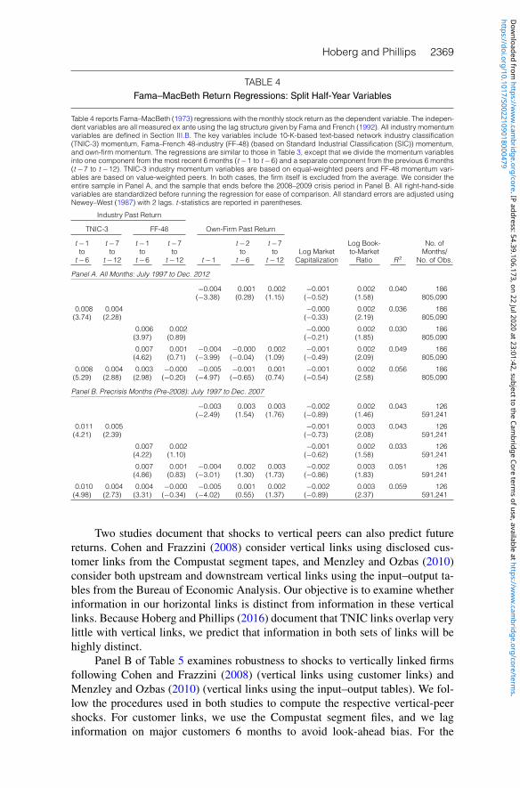
In Table 4, we split the yearly momentum variables into 2 half-year periods.We examine these splits to examine the relative decay rate of momentum. Theregressions are similar to those in Table 3, except that we divide the momentum
https://doi.org/10.1017/S0022109018000479D
ownloaded from
https://ww
w.cam
bridge.org/core . IP address: 54.39.106.173 , on 22 Jul 2020 at 23:01:42 , subject to the Cambridge Core term
s of use, available at https://ww
w.cam
bridge.org/core/terms .

2368 Journal of Financial and Quantitative Analysis
TABLE 3Fama–MacBeth Return Regressions: Various 1-Year Momentum Variables
Table 3 reports Fama–MacBeth (1973) regressions with the monthly stock return as the dependent variable. The indepen-dent variables are all measured ex ante using the lag structure given by Fama and French (1992). All industry momentumvariables are defined in Section III.B. The key variables include 10-K-based text-based network industry classification(TNIC-3) momentum, Fama–French 48-industry (FF-48) (based on Standard Industrial Classification (SIC)) momentum,and own-firm momentum. Both industry momentum variables are based on the past return window t −1 to t −12, andthe own-firm momentum variable skips the most recent month (consistent with other studies); we separately consider themost recent month (known as the reversal variable). TNIC-3 industry momentum variables are based on equal-weightedpeers and FF-48 momentum variables are based on value-weighted peers. In both cases, the firm itself is excluded fromthe average. We consider the entire sample in Panel A, and the sample that ends before the 2008–2009 crisis period inPanel B. All right-hand-side variables are standardized before running the regression for ease of comparison. All standarderrors are adjusted using Newey–West (1987) with 2 lags. t -statistics are reported in parentheses.
Industry Past ReturnOwn-Firm Past Return
TNIC-3 FF-48t −1 t −1 t −2 Log Book- No. ofto to to Log Market to-Market Months/
t −12 t −12 t −1 t −12 Capitalization Ratio R 2 No. of Obs.
Panel A. All Months: July 1997 to Dec. 2012
−0.004 0.001 −0.000 0.002 0.035 186(−3.19) (0.52) (−0.35) (1.57) 805,090
0.008 −0.000 0.002 0.031 186(3.07) (−0.27) (1.99) 805,090
0.005 −0.000 0.002 0.026 186(2.60) (−0.18) (1.66) 805,090
0.006 −0.004 0.001 −0.000 0.002 0.041 186(2.84) (−3.54) (0.28) (−0.30) (1.88) 805,090
0.008 0.003 −0.004 −0.000 −0.000 0.002 0.047 186(4.36) (1.65) (−4.26) (−0.18) (−0.35) (2.30) 805,090
Panel B. Precrisis Months (Pre-2008): July 1997 to Dec. 2007
−0.003 0.004 −0.001 0.003 0.037 126(−2.33) (2.16) (−0.74) (1.43) 591,241
0.011 −0.001 0.003 0.037 126(3.55) (−0.67) (1.89) 591,241
0.007 −0.001 0.003 0.030 126(2.73) (−0.59) (1.49) 591,241
0.006 −0.004 0.004 −0.001 0.003 0.044 126(2.74) (−2.66) (2.03) (−0.70) (1.71) 591,241
0.009 0.003 −0.004 0.002 −0.001 0.003 0.050 126(4.15) (1.56) (−3.40) (1.36) (−0.73) (2.17) 591,241
variables into one component from the most recent 6 months (t−1 to t−6) and aseparate component from the previous 6 months (t−7 to t−12). In the columns,we consider the entire sample and the sample that ends before the 2008–2009crisis period.
The results show that industry TNIC momentum persists into the longermonthly period t−7 to t−12, whereas the FF-48 industry past returns and theown-firm past returns matter only for the first 6 months. These findings stronglysuggest that the information contained in TNIC peer returns is less visible to mar-ket participants, supporting the explanation of slow industry dissemination.
A. Bid–Ask Bounce, Vertical Links, and Simultaneous ReturnsIn Table 5, we consider three robustness tests to the base line specification of
Table 3. Panel A examines robustness to the bid–ask bounce critique, as in Grundyand Martin (2001). For this test, we divide each industry momentum variable intotwo parts: an 11-month term (t−2 to t−12) and a 1-month term (t−1).
https://doi.org/10.1017/S0022109018000479D
ownloaded from
https://ww
w.cam
bridge.org/core . IP address: 54.39.106.173 , on 22 Jul 2020 at 23:01:42 , subject to the Cambridge Core term
s of use, available at https://ww
w.cam
bridge.org/core/terms .
Hoberg and Phillips 2369
TABLE 4Fama–MacBeth Return Regressions: Split Half-Year Variables
Table 4 reports Fama–MacBeth (1973) regressions with the monthly stock return as the dependent variable. The indepen-dent variables are all measured ex ante using the lag structure given by Fama and French (1992). All industry momentumvariables are defined in Section III.B. The key variables include 10-K-based text-based network industry classification(TNIC-3) momentum, Fama–French 48-industry (FF-48) (based on Standard Industrial Classification (SIC)) momentum,and own-firm momentum. The regressions are similar to those in Table 3, except that we divide the momentum variablesinto one component from the most recent 6 months (t −1 to t −6) and a separate component from the previous 6 months(t −7 to t −12). TNIC-3 industry momentum variables are based on equal-weighted peers and FF-48 momentum vari-ables are based on value-weighted peers. In both cases, the firm itself is excluded from the average. We consider theentire sample in Panel A, and the sample that ends before the 2008–2009 crisis period in Panel B. All right-hand-sidevariables are standardized before running the regression for ease of comparison. All standard errors are adjusted usingNewey–West (1987) with 2 lags. t -statistics are reported in parentheses.
Industry Past Return
TNIC-3 FF-48 Own-Firm Past Return
t −1 t −7 t −1 t −7 t −2 t −7 Log Book- No. ofto to to to to to Log Market to-Market Months/
t −6 t −12 t −6 t −12 t −1 t −6 t −12 Capitalization Ratio R 2 No. of Obs.
Panel A. All Months: July 1997 to Dec. 2012
−0.004 0.001 0.002 −0.001 0.002 0.040 186(−3.38) (0.28) (1.15) (−0.52) (1.58) 805,090
0.008 0.004 −0.000 0.002 0.036 186(3.74) (2.28) (−0.33) (2.19) 805,090
0.006 0.002 −0.000 0.002 0.030 186(3.97) (0.89) (−0.21) (1.85) 805,090
0.007 0.001 −0.004 −0.000 0.002 −0.001 0.002 0.049 186(4.62) (0.71) (−3.99) (−0.04) (1.09) (−0.49) (2.09) 805,090
0.008 0.004 0.003 −0.000 −0.005 −0.001 0.001 −0.001 0.002 0.056 186(5.29) (2.88) (2.98) (−0.20) (−4.97) (−0.65) (0.74) (−0.54) (2.58) 805,090
Panel B. Precrisis Months (Pre-2008): July 1997 to Dec. 2007
−0.003 0.003 0.003 −0.002 0.002 0.043 126(−2.49) (1.54) (1.76) (−0.89) (1.46) 591,241
0.011 0.005 −0.001 0.003 0.043 126(4.21) (2.39) (−0.73) (2.08) 591,241
0.007 0.002 −0.001 0.002 0.033 126(4.22) (1.10) (−0.62) (1.58) 591,241
0.007 0.001 −0.004 0.002 0.003 −0.002 0.003 0.051 126(4.86) (0.83) (−3.01) (1.30) (1.73) (−0.86) (1.83) 591,241
0.010 0.004 0.004 −0.000 −0.005 0.001 0.002 −0.002 0.003 0.059 126(4.98) (2.73) (3.31) (−0.34) (−4.02) (0.55) (1.37) (−0.89) (2.37) 591,241
Two studies document that shocks to vertical peers can also predict futurereturns. Cohen and Frazzini (2008) consider vertical links using disclosed cus-tomer links from the Compustat segment tapes, and Menzley and Ozbas (2010)consider both upstream and downstream vertical links using the input–output ta-bles from the Bureau of Economic Analysis. Our objective is to examine whetherinformation in our horizontal links is distinct from information in these verticallinks. Because Hoberg and Phillips (2016) document that TNIC links overlap verylittle with vertical links, we predict that information in both sets of links will behighly distinct.
Panel B of Table 5 examines robustness to shocks to vertically linked firmsfollowing Cohen and Frazzini (2008) (vertical links using customer links) andMenzley and Ozbas (2010) (vertical links using the input–output tables). We fol-low the procedures used in both studies to compute the respective vertical-peershocks. For customer links, we use the Compustat segment files, and we laginformation on major customers 6 months to avoid look-ahead bias. For the
https://doi.org/10.1017/S0022109018000479D
ownloaded from
https://ww
w.cam
bridge.org/core . IP address: 54.39.106.173 , on 22 Jul 2020 at 23:01:42 , subject to the Cambridge Core term
s of use, available at https://ww
w.cam
bridge.org/core/terms .

2370 Journal of Financial and Quantitative Analysis
TABLE 5Fama–MacBeth Return Regressions:
Bid–Ask Bounce, Vertical Links, and Simultaneous Returns
Table 5 reports Fama–MacBeth (1973) regressions with the monthly stock return as the dependent variable. The indepen-dent variables are all measured ex ante using the lag structure given by Fama and French (1992). All industry momentumvariables are defined in Section III.B. We consider 3 robustness tests that use the same baseline specifications in Table 3,although each with one change meant to zoom in on a particular robustness issue. Panel A examines robustness to thebid–ask bounce critique as in Grundy and Martin (2001). Hence, we divide each industry momentum variable into 2parts: an 11-month term (t −2 to t −12) and a 1-month term (t −1). Panel B examines robustness to shocks to verticallylinked firms following Cohen and Frazzini (2008) (vertical links using customer links) and Menzley and Ozbas (2010)(vertical links using the input–output tables (IO tables)). We follow the procedures used in both studies to compute therespective vertical-peer shocks. For customer links, we use the Compustat segment files, and we lag information on ma-jor customers 6 months to avoid look-ahead bias. For IO table vertical-peer returns, we use the 1997 and 2002 IO tablesgiven that we predict returns from July 1997 forward. Panel C examines robustness to including controls for simultaneoustext-based network industry classification (TNIC-3) and Fama–French 48-industry (FF-48) returns measured in the sameperiod as the dependent variable (month t ). In the sample column, we note that we consider the entire sample, and thesample that ends before the 2008–2009 crisis period. All right-hand-side variables are standardized before running theregression for ease of comparison. All standard errors are adjusted using Newey–West (1987) with 2 lags. t -statistics arereported in parentheses.
Panel A. Robustness to Bid–Ask BouncePast Return
t −2 to t −11 t −1t −2 to
Industry t −12 Industry
Sample TNIC-3 FF-48 Own Firm TNIC-3 FF-48 Own Firm
All 0.005 0.000 0.010 −0.005(2.85) (0.04) (7.99) (−5.35)
All 0.002 0.001 0.012 −0.005(1.15) (0.39) (6.86) (−4.66)
All 0.006 −0.001 0.000 0.008 0.008 −0.005(3.95) (−0.59) (0.06) (8.41) (5.34) (−5.70)
Pre-2008 0.007 0.002 0.011 −0.005(3.15) (1.64) (7.33) (−4.30)
Pre-2008 0.003 0.004 0.014 −0.004(1.60) (2.17) (6.72) (−3.59)
Pre-2008 0.007 −0.001 0.002 0.009 0.009 −0.005(3.83) (−0.53) (1.67) (7.65) (5.34) (−4.57)
Panel B. Robustness to Vertical Economic Links
Past Return
Industry Vertical
t −1 to t −12 t −2 to t −12 t −1
Sample TNIC-3 FF-48 Customer IO Table Customer IO Table
All 0.008 0.003 0.001 −0.004 0.001 0.006(4.64) (1.94) (1.73) (−1.56) (1.96) (2.17)
Pre-2008 0.009 0.003 0.001 −0.003 0.001 0.007(4.26) (1.96) (2.17) (−1.34) (1.50) (2.60)
Panel C. Robustness to Simultaneous Returns
Past Return
Industry Industry ReturnOwn Firm
t −1 to t −12 Simultaneoust −2 to
Sample TNIC-3 FF-48 t −12 t −1 TNIC-3 FF-48
All 0.014 0.003 −0.001 −0.005 0.034 0.021(6.37) (0.86) (−0.27) (−5.75) (35.24) (22.86)
Pre-2008 0.013 0.000 0.002 −0.005 0.034 0.018(4.98) (0.18) (1.25) (−4.66) (28.15) (17.30)
input–output table vertical-peer returns, we use the 1997 and 2002 input–outputtables given that we predict returns from July 1997 forward. Second, we computethe average returns separately for both upstream and downstream industries for
https://doi.org/10.1017/S0022109018000479D
ownloaded from
https://ww
w.cam
bridge.org/core . IP address: 54.39.106.173 , on 22 Jul 2020 at 23:01:42 , subject to the Cambridge Core term
s of use, available at https://ww
w.cam
bridge.org/core/terms .

Hoberg and Phillips 2371
the same 2 return windows. Third, we compute the average of the upstream anddownstream peer returns for both return windows. We then reconsider the regres-sions in Table 3 including these 4 additional control variables (2 horizons, 2 typesof vertical links).
Panel C of Table 5 examines robustness to including controls for simultane-ous TNIC-3 and FF-48 monthly industry returns measured in the same period asthe dependent variable (month t).
Panel A of Table 5 shows that our results are robust to the bid–ask bouncecritique. Our TNIC past industry return measured from t−2 to t−12 remainshighly significant. However, the table also shows, consistent with Grundy andMartin (2001), that SIC-based FF-48 momentum generally loses significance inthis specification.
Panel B of Table 5 shows that our TNIC-3 past return variables are alsohighly robust to including the 4 vertical link variables. We are able to replicatethe main results in both Cohen and Frazzini (2008) and Menzley and Ozbas(2010). For example, the shock to customers is positive and significant in mostspecifications. We also find that the input–output table vertical return is positiveand significant at the shorter 1-month horizon.
We standardize all RHS variables in the regressions to have a 0 mean and aunit variance before running the regressions in Table 5. Hence, the coefficientscan be compared and conclusions can be drawn regarding relative economicmagnitudes. The table shows that the coefficients for TNIC-3 momentum arenearly a full order of magnitude larger than the vertical-peer coefficients for thelong horizon, which is the standard horizon used to assess momentum. We con-clude that shocks to both vertical and horizontal firms can independently predictreturns, although shocks to horizontal peers are far more likely to explain mo-mentum than are shocks to vertical peers. This statement is particularly true forthe less visible TNIC peer links.
Finally, Panel C of Table 5 shows that our TNIC industry past return remainssignificant when including simultaneous TNIC-3 and FF-48 returns.
B. Various HorizonsWe consider various horizons of the momentum variables. In particular, we
consider 3-, 6-, 12-, and 24-month past returns. Panel A of Table 6 displays resultsfor the full sample and shows that TNIC momentum is highly significant evenat longer horizons up to 1 year. In contrast, FF-48 momentum is not significantbeyond the 6-month horizon. The results for the FF-48 peers overall are smallerin magnitude and more short-lived.
The independent variables in our regressions are standardized before runningthe regressions, and the coefficients are interpretable. The 6-month economic im-pact of FF-48 peer peers (monthly return of 0.004 per sigma unit) is only halfthat of TNIC-3 peers at the same horizon (0.008). Moreover, TNIC-3 returnscontinue to accumulate returns, with a total summed coefficient of 0.013 overthe 1-year horizon. FF-48 coefficients do not accumulate beyond 0.005. Thesefindings suggest that the market more efficiently prices shocks to more visiblepeers. Our results are also robust during the broader sample, which includes thefinancial crisis, and the shorter sample, which ends in 2007. This is expected
https://doi.org/10.1017/S0022109018000479D
ownloaded from
https://ww
w.cam
bridge.org/core . IP address: 54.39.106.173 , on 22 Jul 2020 at 23:01:42 , subject to the Cambridge Core term
s of use, available at https://ww
w.cam
bridge.org/core/terms .

2372 Journal of Financial and Quantitative Analysis
TABLE 6Fama–MacBeth Return Regressions: Various Momentum Horizons
Table 6 reports Fama–MacBeth (1973) regressions with the monthly stock return as the dependent variable. The indepen-dent variables are all measured ex ante using the lag structure given by Fama and French (1992). All industry momentumvariables are defined in Section III.B. The key variables include own-firm momentum, Fama–French 48-industry (FF-48)(based on Standard Industrial Classification (SIC)) momentum, and 10-K-based text-based network industry classifica-tion (TNIC-3) momentum. We consider momentum horizons that range from months t −1 to t −6 for short horizons andmonths t −13 to t −24 for longer horizons. TNIC-3 industry momentum variables are based on equal-weighted peersand FF-48 momentum variables are based on value-weighted peers. In both cases, the firm itself is excluded from theaverage. We also include controls for size and book-to-market. We consider the entire sample in Panel A, and the samplethat ends before the 2008–2009 crisis period in Panel B. All right-hand-side variables are standardized before runningthe regression for ease of comparison. All standard errors are adjusted using Newey–West (1987) with 2 lags. t -statisticsare reported in parentheses.
Past Return
Industry Log Book- No. ofOwn Log Market to-Market Months/
Momentum Duration TNIC-3 FF-48 Firm Capitalization Ratio R 2 No. of Obs.
Panel A. All Months: July 1997 to Dec. 2012
Months 1–6 0.008 0.004 −0.001 −0.001 0.002 0.039 186(4.58) (3.41) (−0.56) (−0.46) (2.13) 805,090
Months 7–12 0.005 0.001 0.001 −0.001 0.002 0.033 186(2.93) (0.40) (0.88) (−0.42) (1.76) 805,090
Months 13–24 −0.002 −0.001 −0.002 −0.000 0.001 0.030 186(−1.17) (−0.44) (−2.04) (−0.33) (0.70) 762,400
Panel B. Precrisis Months (Pre-2008): July 1997 to Dec. 2007
Months 1–6 0.010 0.005 0.001 −0.001 0.003 0.043 126(4.41) (3.81) (0.87) (−0.82) (1.93) 591,241
Months 7–12 0.006 0.001 0.002 −0.002 0.002 0.036 126(3.02) (0.60) (1.45) (−0.77) (1.54) 591,241
Months 13–24 −0.001 −0.000 −0.002 −0.001 0.001 0.036 126(−0.37) (−0.24) (−1.60) (−0.77) (0.57) 556,149
under our hypothesis that states momentum is due to inattention and not system-atic risk.
C. Product Market BreadthDoes momentum arise from shocks to more localized peers in the product
market space (we refer to such shocks as “local”) or broader shocks affectinglarger numbers of product market peers (we refer to such shocks as “broad”)? Wenote the use of terms such as “local” and “broad” are intended to have a spatialinterpretation as the TNIC industry classification can be viewed as a product mar-ket space shaped as a high dimensional sphere (see Hoberg and Phillips (2016)).Local peer shocks affect only a small region of the space around a firm, and broadpeer shocks affect wide swaths of space around a firm. This question is partic-ularly interesting because a theory of systematic risk predicts that only broadshocks affecting many firms will be priced. If this is not the case, peer shockswould be easy to diversify, and in equilibrium, investors would not demand riskpremia for investing in firms exposed to diversifiable shocks.
In contrast, the inattention hypothesis states that shocks to local productmarket peers are be more important. A key reason is that broad shocks that af-fect large numbers of firms are more visible and hence are less susceptible toinattention–driven anomalies. In contrast, local product market shocks are not asvisible and are more idiosyncratic, and hence, the inattention hypothesis predictslarger momentum returns.
https://doi.org/10.1017/S0022109018000479D
ownloaded from
https://ww
w.cam
bridge.org/core . IP address: 54.39.106.173 , on 22 Jul 2020 at 23:01:42 , subject to the Cambridge Core term
s of use, available at https://ww
w.cam
bridge.org/core/terms .

Hoberg and Phillips 2373
In Table 7, we consider peers positioned in the product market in differentdistance bands around a given focal firm. For example, our first distance bandincludes the most local peers, defined as peers with textual cosine similarity toa given focal firm that is in the highest 1.05% of all pairwise similarities. Thisthreshold is equally as granular as firms appearing in the same SIC-4 code, andthus firms in this band are highly similar. Our second distance band includes firmsthat are not in the 1.05% most similar peers but are in the 2.03% most similarpeers. This threshold is analogous to firms that are in the same SIC-3 code butare not in the same SIC-4 code. Intuitively, peers in this second group are broaderin the product market space than peers in the first band. Our third distance bandincludes firms that are as proximate in the TNIC industry space as are SIC-2pairs (4.52%) but not as proximate as SIC-3 pairs (2.03%). Finally, our broadestdistance band includes firms that are as proximate in the TNIC industry space asare SIC-1 pairs (15.8%) but not as proximate as SIC-2 pairs (4.52%).
We consider shocks to these distance-based peer groups as competing RHSvariables in our standard Fama–MacBeth (1973) setting. All momentum variablesare based on peer returns using the standard 12-month horizon from t−12 to t−1.As before, we consider the full sample in Panel A of Table 7, and a sample thatexcludes the financial crisis period in Panel B. The table shows that shocks toproduct market peers drive momentum only when the peers are local. The inner
TABLE 7Fama–MacBeth Return Regressions: Industry Breadth
Table 7 reports Fama–MacBeth (1973) regressions with the monthly stock return as the dependent variable. The indepen-dent variables are all measured ex ante using the lag structure given by Fama and French (1992). All industry momentumvariables are defined in Section III.B. We compute text-based network industry classification (TNIC) momentum usingvarious granularities as noted in the first column: TNIC-4 (analogous to 4-digit Standard Industrial Classification (SIC-4)), TNIC-(3-4) (analogous to being in SIC-3 but not SIC-4), TNIC-(2-3) (analogous to being in SIC-2 but not SIC-3),and TNIC-(1-2) (analogous to being in SIC-1 but not SIC-2). We consider the past 12-month returns for each. Industrymomentum variables are based on the equal-weighted average past returns of rival firms in each industry where thefirm itself is excluded from the average. We also include controls for own-firm momentum, Fama–French 48-industry(FF-48) momentum, size, and book-to-market. We consider the entire sample in Panel A, and the sample that ends be-fore the 2008–2009 crisis period in Panel B. All right-hand-side variables are standardized before running the regressionfor ease of comparison. All standard errors are adjusted using Newey–West (1987) with 2 lags. t -statistics are reportedin parentheses.
Industry Past Return
t −2 to t −1 tot −1 to t −12 t −12 t −12 t −1 No. of
Log Book- Months/Own Own Log Market to-Market No. of
TNIC-4 TNIC-(3-4) TNIC-(2-3) TNIC-(1-2) Firm FF-48 Firm Capitalization Ratio R 2 Obs.
Panel A. All Months: July 1997 to Dec. 2012
0.005 0.004 0.001 −0.001 −0.004 −0.000 0.002 0.044 186(4.79) (4.09) (0.75) (−0.32) (−4.23) (−0.26) (2.29) 805,090
0.005 0.004 0.001 −0.001 −0.001 0.008 −0.004 −0.000 0.002 0.051 186(6.05) (4.36) (0.54) (−0.22) (−0.23) (1.56) (−4.47) (−0.39) (2.56) 805,090
0.005 0.004 −0.001 0.009 −0.004 −0.001 0.002 0.047 186(5.51) (3.08) (−0.24) (1.64) (−4.26) (−0.39) (2.25) 805,090
Panel B. Precrisis Months (Pre-2008): July 1997 to Dec. 2007
0.006 0.005 0.002 −0.002 −0.004 −0.001 0.003 0.050 126(5.11) (4.52) (1.36) (−0.59) (−3.51) (−0.62) (2.32) 591,241
0.006 0.005 0.001 −0.001 0.002 0.002 −0.004 −0.001 0.003 0.055 126(5.71) (4.43) (0.98) (−0.47) (1.30) (1.51) (−3.62) (−0.74) (2.51) 591,241
0.006 0.005 0.002 0.002 −0.004 −0.001 0.003 0.051 126(5.02) (3.06) (1.29) (1.54) (−3.39) (−0.77) (2.11) 591,241
https://doi.org/10.1017/S0022109018000479D
ownloaded from
https://ww
w.cam
bridge.org/core . IP address: 54.39.106.173 , on 22 Jul 2020 at 23:01:42 , subject to the Cambridge Core term
s of use, available at https://ww
w.cam
bridge.org/core/terms .

2374 Journal of Financial and Quantitative Analysis
band is highly significant in predicting ex post returns, as is the second band.However, neither of the broader bands is statistically significant.
We conclude that peers located in the product market space with proximitysimilar to SIC-4 and SIC-3 peers (analogous to the 2% most similar firm pairsamong all pairs) generate long-term momentum. This finding is not consistentwith an explanation for momentum based on systematic risk, as shocks to peersthat are this local should be relatively easy to diversify. Our results thus favor thevisibility and inattention hypothesis for industry momentum.
D. Idiosyncratic and Systematic RiskIn this section, we decompose our momentum variables into a component
that is due to systematic risk and a component that is due to idiosyncratic risk. Weuse the decomposition methods discussed in Section III.D. We use projections ofdaily stock returns onto the daily Fama–French (1992) factors plus momentum(UMD) and then tabulate the total contribution of systematic risk projections toeach firm’s monthly return. Next, we compute peer momentum variables usingour standard averaging approach. Finally, we define the idiosyncratic componentas the raw peer return minus the systematic peer return component.
Table 8 displays results for our standard asset pricing regressions, with boththe TNIC-3 idiosyncratic peer return and the systematic peer return as RHSvariables. We consider 2 horizons: the near-term horizon of t−1 to t−6 and alonger term horizon of t−7 to t−12. Panel A presents results for the full sampleand Panel B for the subsample that excludes the financial crisis.
Table 8 shows that for long-term momentum for the t−7 to t−12 horizonin columns 3 and 4, only idiosyncratic peer shocks matter. Even for the shorter6-month horizon in columns 1 and 2, the idiosyncratic component (highly sig-nificant at the 1% level in all 4 specifications) strongly dominates the systematiccomponent (significant in only 2 of the specifications at the 5% level and insignif-icant in the other 2 specifications). These results reinforce our earlier findingsas discussed in Table A3 of the Supplementary Material, but in a more stark,long-horizon fashion. Whereas systematic peer returns do create some modest re-turn predictability lasting 1–2 months, they create no return predictability beyondthis horizon. Idiosyncratic returns generate predictability for at least 1 year. Weconclude that the industry momentum anomaly is likely due to more localized id-iosyncratic peer shocks affecting a smaller fraction of firms in the economy, whichis also consistent with a low-visibility interpretation given that fewer investors payattention any specific localized shock and more investors pay attention to largerand more systematic shocks.
E. TNIC and SIC DisparityIn this section, we consider how firms that are in the TNIC network, but
are not in the same SIC code, might drive our results. We note that for somefirms, these peers are highly concordant, and for others, TNIC-3 peers differsubstantially from SIC-3 peers. Under the inattention hypothesis, we expect long-term momentum returns to be sharpest for firms that have high disparity across the2 sets of peers. We thus compute “disparity” as 1 minus the total sales of firms thatare at the intersection of TNIC-3 peers and SIC-3 peer groups divided by the total
https://doi.org/10.1017/S0022109018000479D
ownloaded from
https://ww
w.cam
bridge.org/core . IP address: 54.39.106.173 , on 22 Jul 2020 at 23:01:42 , subject to the Cambridge Core term
s of use, available at https://ww
w.cam
bridge.org/core/terms .

Hoberg and Phillips 2375
TABLE 8Fama–MacBeth Return Regressions: Idiosyncratic and Systematic Risk
Table 8 reports Fama–MacBeth (1973) regressions with the monthly stock return as the dependent variable. The inde-pendent variables include momentum variables based on the systematic and idiosyncratic portions of the text-basedreturn benchmark. Industry momentum variables are defined in Section III.B. To compute the systematic portion, we firstregress (for each month) daily stock returns for each firm onto the 3 Fama and French (1992) factors and the momentumfactor. The projection from this regression (excluding the projection from the intercept) is the systematic portion of a firm’sdaily return. These are then aggregated to monthly observations, and we compute the value-weighted average of thesesystematic returns over each firm’s text-based peers to get the systematic peer return. The idiosyncratic peer return is theraw text-based peer return minus the systematic peer return. Text-based network industry classification (TNIC-3) momen-tum variables are based on the equal-weighted average past returns of rival firms in each TNIC industry where the firmitself is excluded from the average. We also include controls for size and book-to-market. We consider the entire samplein Panel A, and the sample that ends before the 2008–2009 crisis period in Panel B. All right-hand-side variables arestandardized before running the regression for ease of comparison. All standard errors are adjusted using Newey–West(1987) with 2 lags. t -statistics are reported in parentheses.
TNIC-3 Industry Past Return
t −1 to t −6 t −7 to t −12 Log Book- No. ofLog Market to-Market Months/
Idiosyncratic Systematic Idiosyncratic Systematic Capitalization Ratio R 2 No. of Obs.
Panel A. All Months: July 1997 to Dec. 2012
0.007 0.004 0.004 0.002 −0.000 0.002 0.041 186(4.39) (1.97) (3.05) (1.40) (−0.37) (2.28) 805,090
0.006 0.003 −0.000 0.002 0.027 186(4.13) (3.36) (−0.13) (2.14) 805,090
0.001 0.000 −0.000 0.002 0.029 186(0.44) (0.11) (−0.33) (1.53) 805,090
Panel B. Precrisis Months: July 1997 to Dec. 2007
0.009 0.006 0.005 0.002 −0.001 0.003 0.047 126(4.91) (2.69) (3.49) (1.17) (−0.72) (2.26) 591,241
0.008 0.004 −0.001 0.003 0.032 126(4.39) (3.13) (−0.55) (2.06) 591,241
0.002 −0.000 −0.001 0.002 0.034 126(1.11) (−0.27) (−0.67) (1.41) 591,241
sales of firms in the union of TNIC-3 and SIC-3 peers. This variable is boundedin the range [0,1], and a high value indicates that an investor relying on SIC-3classifications would miss a large fraction of information about product marketpeers. Hence, we hypothesize that firms with high disparity are more susceptibleto momentum under the hypothesis that momentum is driven by inattention andless visible economic links.
Our main specification in Table 3 focuses on momentum for both the near-term horizon of t−1 to t−6 and the longer term horizon of t−7 to t−12. InTable 9, we rerun this model for firms in different quintiles based on their industrydisparity. Panel A presents results for the full sample and Panel B for the subsam-ple that excludes the financial crisis. Our hypothesis is that momentum variablesare stronger in high-disparity quintiles and weaker in low-disparity quintiles.
The results in both panels for the longer t−7 to t−12 horizon stronglysupport the hypothesis that momentum is stronger for firms with more TNICrather than SIC-based industry peers. The long-horizon momentum variable ispositive and significant at the 1% level and highly economically significant inhigh-disparity quintiles. In contrast, it has a much smaller magnitude and is notsignificant in the low-disparity quintile. We observe similar but less striking sortsby disparity for the shorter t−1 to t−6 horizon. The fact that the longer horizonsorts by disparity more than does the short horizon is further consistent with avisibility interpretation, as it indicates that return shocks disseminate most slowly
https://doi.org/10.1017/S0022109018000479D
ownloaded from
https://ww
w.cam
bridge.org/core . IP address: 54.39.106.173 , on 22 Jul 2020 at 23:01:42 , subject to the Cambridge Core term
s of use, available at https://ww
w.cam
bridge.org/core/terms .
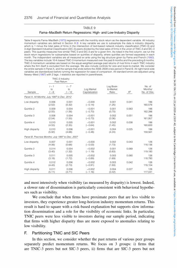
2376 Journal of Financial and Quantitative Analysis
TABLE 9Fama–MacBeth Return Regressions: High- and Low-Industry Disparity
Table 9 reports Fama–MacBeth (1973) regressions with the monthly stock return as the dependent variable. All industrymomentum variables are defined in Section III.B. A key variable we use to subsample the data is industry disparity,which is 1 minus the total sales of firms in the intersection of text-based network industry classification (TNIC-3) and3-digit Standard Industrial Classification (SIC-3) peers divided by the total sales of firms in the union of TNIC-3 and SIC-3peers. This quantity measures how similar TNIC-3 and SIC-3 are for a given firm. As noted in the first column, we run thestock return regressions for subsamples based on quintiles of disparity, where quintiles are formed separately in eachmonth. The independent variables are all measured ex ante using the lag structure given by Fama and French (1992).The key variables include 10-K-based TNIC-3 momentummeasured over the past 6 months and the preceding 6 months.TNIC-3 momentum variables are based on the equal-weighted average past returns of rival firms in each TNIC industrywhere the firm itself is excluded from the average. We also include controls for size and book-to-market. We considerthe entire sample in Panel A, and the sample that ends before the 2008–2009 crisis period in Panel B. All right-hand-sidevariables are standardized before running the regression for ease of comparison. All standard errors are adjusted usingNewey–West (1987) with 2 lags. t -statistics are reported in parentheses.
TNIC-3 IndustryPast Return
t −1 t −7 Log Book- No. ofto to Log Market to-Market Months/
Sample t −6 t −12 Capitalization Ratio R 2 No. of Obs.
Panel A. All Months: July 1997 to Dec. 2012
Low disparity 0.006 0.001 −0.000 0.001 0.041 186(2.52) (0.32) (−0.14) (1.25) 160,576
Quintile 2 0.009 0.004 −0.001 0.001 0.063 186(2.55) (1.56) (−0.70) (0.70) 162,396
Quintile 3 0.008 0.004 −0.001 0.002 0.051 186(2.54) (1.55) (−0.73) (2.06) 161,957
Quintile 4 0.010 0.005 −0.001 0.002 0.038 186(4.55) (2.35) (−0.64) (1.45) 160,600
High disparity 0.010 0.006 −0.001 0.004 0.025 186(5.92) (4.68) (−0.48) (4.24) 159,561
Panel B. Precrisis Months: July 1997 to Dec. 2007
Low disparity 0.007 0.001 −0.000 0.002 0.043 126(4.06) (0.68) (−0.03) (1.73) 118,136
Quintile 2 0.014 0.004 −0.002 0.001 0.069 126(3.40) (1.32) (−1.19) (0.83) 119,180
Quintile 3 0.011 0.005 −0.002 0.003 0.060 126(3.18) (1.72) (−0.89) (1.69) 118,780
Quintile 4 0.012 0.006 −0.002 0.003 0.042 126(4.43) (2.73) (−0.91) (1.93) 118,104
High disparity 0.011 0.006 −0.002 0.004 0.027 126(5.11) (3.71) (−1.16) (3.42) 117,041
and most intensively when visibility (as measured by disparity) is lowest. Indeed,a slower rate of dissemination is particularly consistent with behavioral hypothe-ses such as visibility.
We conclude that when firms have proximate peers that are less visible toinvestors, they experience greater long-horizon industry momentum returns. Thisresult is hard to square with a risk-based explanation but supports slow informa-tion dissemination and a role for the visibility of economic links. In particular,TNIC peers were less visible to investors during our sample period, indicatingthat firms with higher disparity thus are more exposed to anomalies relating tolow visibility.
F. Partitioning TNIC and SIC PeersIn this section, we consider whether the past returns of various peer groups
separately predict momentum returns. We focus on 3 groups: i) firms thatare TNIC-3 peers but not SIC-3 peers, ii) firms that are SIC-3 peers but not
https://doi.org/10.1017/S0022109018000479D
ownloaded from
https://ww
w.cam
bridge.org/core . IP address: 54.39.106.173 , on 22 Jul 2020 at 23:01:42 , subject to the Cambridge Core term
s of use, available at https://ww
w.cam
bridge.org/core/terms .
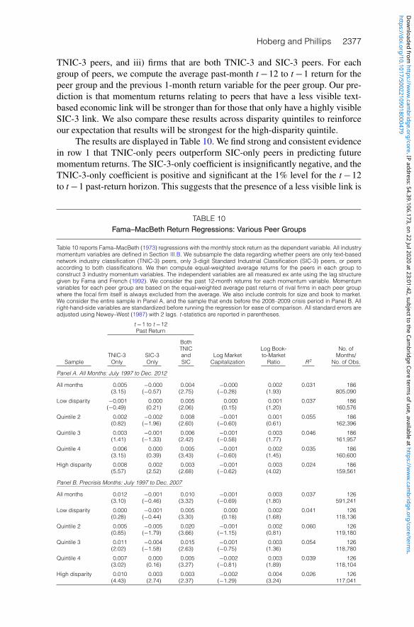
Hoberg and Phillips 2377
TNIC-3 peers, and iii) firms that are both TNIC-3 and SIC-3 peers. For eachgroup of peers, we compute the average past-month t−12 to t−1 return for thepeer group and the previous 1-month return variable for the peer group. Our pre-diction is that momentum returns relating to peers that have a less visible text-based economic link will be stronger than for those that only have a highly visibleSIC-3 link. We also compare these results across disparity quintiles to reinforceour expectation that results will be strongest for the high-disparity quintile.
The results are displayed in Table 10. We find strong and consistent evidencein row 1 that TNIC-only peers outperform SIC-only peers in predicting futuremomentum returns. The SIC-3-only coefficient is insignificantly negative, and theTNIC-3-only coefficient is positive and significant at the 1% level for the t−12to t−1 past-return horizon. This suggests that the presence of a less visible link is
TABLE 10Fama–MacBeth Return Regressions: Various Peer Groups
Table 10 reports Fama–MacBeth (1973) regressions with the monthly stock return as the dependent variable. All industrymomentum variables are defined in Section III.B. We subsample the data regarding whether peers are only text-basednetwork industry classification (TNIC-3) peers, only 3-digit Standard Industrial Classification (SIC-3) peers, or peersaccording to both classifications. We then compute equal-weighted average returns for the peers in each group toconstruct 3 industry momentum variables. The independent variables are all measured ex ante using the lag structuregiven by Fama and French (1992). We consider the past 12-month returns for each momentum variable. Momentumvariables for each peer group are based on the equal-weighted average past returns of rival firms in each peer groupwhere the focal firm itself is always excluded from the average. We also include controls for size and book to market.We consider the entire sample in Panel A, and the sample that ends before the 2008–2009 crisis period in Panel B. Allright-hand-side variables are standardized before running the regression for ease of comparison. All standard errors areadjusted using Newey–West (1987) with 2 lags. t -statistics are reported in parentheses.
t −1 to t −12Past Return
BothTNIC Log Book- No. of
TNIC-3 SIC-3 and Log Market to-Market Months/Sample Only Only SIC Capitalization Ratio R 2 No. of Obs.
Panel A. All Months: July 1997 to Dec. 2012
All months 0.005 −0.000 0.004 −0.000 0.002 0.031 186(3.15) (−0.57) (2.75) (−0.28) (1.93) 805,090
Low disparity −0.001 0.000 0.005 0.000 0.001 0.037 186(−0.49) (0.21) (2.06) (0.15) (1.20) 160,576
Quintile 2 0.002 −0.002 0.008 −0.001 0.001 0.055 186(0.82) (−1.96) (2.60) (−0.60) (0.61) 162,396
Quintile 3 0.003 −0.001 0.006 −0.001 0.003 0.046 186(1.41) (−1.33) (2.42) (−0.58) (1.77) 161,957
Quintile 4 0.006 0.000 0.005 −0.001 0.002 0.035 186(3.15) (0.39) (3.43) (−0.60) (1.45) 160,600
High disparity 0.008 0.002 0.003 −0.001 0.003 0.024 186(5.57) (2.52) (2.68) (−0.62) (4.02) 159,561
Panel B. Precrisis Months: July 1997 to Dec. 2007
All months 0.012 −0.001 0.010 −0.001 0.003 0.037 126(3.10) (−0.46) (3.32) (−0.69) (1.80) 591,241
Low disparity 0.000 −0.001 0.005 0.000 0.002 0.041 126(0.28) (−0.44) (3.30) (0.18) (1.68) 118,136
Quintile 2 0.005 −0.005 0.020 −0.001 0.002 0.060 126(0.85) (−1.79) (3.66) (−1.15) (0.81) 119,180
Quintile 3 0.011 −0.004 0.015 −0.001 0.003 0.054 126(2.02) (−1.58) (2.63) (−0.75) (1.36) 118,780
Quintile 4 0.007 0.000 0.005 −0.002 0.003 0.039 126(3.02) (0.16) (3.27) (−0.81) (1.89) 118,104
High disparity 0.010 0.003 0.003 −0.002 0.004 0.026 126(4.43) (2.74) (2.37) (−1.29) (3.24) 117,041
https://doi.org/10.1017/S0022109018000479D
ownloaded from
https://ww
w.cam
bridge.org/core . IP address: 54.39.106.173 , on 22 Jul 2020 at 23:01:42 , subject to the Cambridge Core term
s of use, available at https://ww
w.cam
bridge.org/core/terms .

2378 Journal of Financial and Quantitative Analysis
more important than the absence of a highly visible link when predicting momen-tum returns. Interestingly, we also find that the both-TNIC-and-SIC peer groupperforms well and produces positive and significant momentum returns. This sug-gests that a firm that is both an SIC and a TNIC peer has a strong economiclink to the firm. As investors are likely inattentive to the TNIC link, they shouldunderreact to the large momentum returns that flow through such ultra-strongpeers as they would not be aware that these peers are stronger than standard SIC-only peers. These findings are robust both in the full sample and in the pre-2008sample.
Table 10 also displays results separately for firms by industry disparity quin-tiles in rows 2–6 for the full sample and 7–12 for the pre-2008 sample. The tableshows strong and nearly monotonic sorting of the TNIC-only coefficient, whichbecomes very large in the high-disparity quintile. We also observe that the FF-48-only peers do not predict momentum returns in a material way in any quintile ex-cept the highest disparity quintile. In contrast, the both-TNIC-and-SIC peer grouppredicts momentum returns in all quintiles. This variable is slightly stronger inlow- to middle-disparity quintiles, where peers that are in both classifications ismore common (given the definition of disparity). In all, the findings support ourconclusion that momentum due to less visible peers predicts strong momentumprofits, whereas highly visible peers do not.
G. Calendar-Time PortfoliosWe next consider whether our results are robust to calendar-time portfolio
methods. For a given momentum variable (TNIC-3 based, FF-48 based, or ownfirm based), we first sort firms into quintiles based on the given variable separatelyin each month. For all industry momentum returns, we focus on the standard hori-zon of t−1 to t−12. For own-firm momentum, consistent with the literature, wefocus on the 11-month horizon from t−2 to t−12.
We then compute the returns of equal-weighted portfolios that i) invest longin the highest quintile firms and ii) invest short in the lowest quintile firms. Wethus have a consistent way of computing the returns of zero-cost portfolios for anymomentum variable. In the second stage, we regress the returns of our zero-costportfolios on the market factor, HML, SMB, and, in some specifications, the UMDfactor.5 Our primary test is whether the intercept (which we refer to as “alpha”) isstatistically and economically distinct from 0.
In Panel A of Table 11, we compute the zero-cost portfolios based only on thesubsample of firms in the high-disparity quintile. We expect predictable returnsto be particularly high in this subsample, and we focus on TNIC-3 momentumas the momentum sort variable. In rows 1–2, we consider the full sample fromJuly 1997 to Dec. 2012; row 1 omits the UMD factor whereas row 2 includes theUMD factor. We note that the alpha is statistically significant with a t-statistic thatexceeds 5.0 in all 4 specifications. Economically, we observe predictable returnsthat range from 1.9% to 2.3% per month for the full sample, and 1.8% to 2.7%for the sample that excludes the financial crisis. We find Sharpe ratios that range
5We thank Kenneth French for providing factor data on his Web site.
https://doi.org/10.1017/S0022109018000479D
ownloaded from
https://ww
w.cam
bridge.org/core . IP address: 54.39.106.173 , on 22 Jul 2020 at 23:01:42 , subject to the Cambridge Core term
s of use, available at https://ww
w.cam
bridge.org/core/terms .

Hoberg and Phillips 2379
TABLE 11Calendar-Time Portfolios: Equal-Weighted Black–Jensen–Scholes (BJS) Alpha Test
Table 11 reports ordinary least squares (OLS) coefficients and factor loadings based on calendar-time zero-investmentportfolios investing long in positive momentum stocks and short in negative momentum stocks. All portfolios are equalweighted. The portfolios are constructed from varying definitions of momentum: text-based network industry classification(TNIC-3) momentum (Panels A and B), Fama–French 48-industry (FF-48) (based on Standard Industrial Classification(SIC)) momentum (Panel C), and own momentum (Panel D). All industry momentum variables are defined in Section III.B.All tests are based on the full sample except Panel A, which is based on portfolios of stocks in the highest quintile ofindustry disparity (1 minus the total sales of all firms in the intersection of TNIC-3 and 3-digit SIC (SIC-3) peer groups,divided by the total sales of firms in the union of the given firm’s TNIC-3 and SIC-3 industries). We consider a 1-yearmeasurement period for past returns as noted in the first column. For own-firm momentum, we skip the most recentmonth, following the literature. Zero-investment calendar-time portfolios are constructed by first sorting firms into quintilesbased on the given momentum variables in each month. We then compute equal-weighted average returns of firms inthe highest quintile and subtract the equal-weighted returns of firms in the lowest quintile. Annualized Sharpe ratios arecomputed as the square root of 12 times the monthly mean divided by the monthly standard deviation. We report theSharpe ratio of the raw return (top) and the residual return (bottom) for each specification. t -statistics are reported inparentheses.
Sample/ Sharpe No. ofHorizon Alpha MKT HML SMB UMD Ratios R 2 Obs.
Panel A. 10-K Based TNIC-3 Momentum (High-Disparity Quintile)
All months 0.023 −0.259 −0.280 0.530 1.432 0.195 186t −1 to t −12 momentum (6.18) (−3.28) (−2.50) (4.91) 1.603
All months 0.019 0.039 −0.073 0.393 0.653 1.432 0.613 186t −1 to t −12 momentum (7.29) (0.66) (−0.92) (5.20) (13.99) 1.908
Pre-2008 0.027 −0.333 −0.272 0.638 1.424 0.242 126t −1 to t −12 momentum (5.22) (−2.54) (−1.57) (4.67) 1.680
Pre-2008 0.018 0.025 −0.095 0.407 0.835 1.424 0.722 126t −1 to t −12 momentum (5.68) (0.29) (−0.90) (4.81) (14.46) 1.868
Panel B. 10-K-Based TNIC-3 Momentum
All months 0.017 −0.386 −0.285 0.611 0.777 0.146 186t −1 to t −12 momentum (3.30) (−3.50) (−1.82) (4.05) 0.857
All months 0.011 0.099 0.051 0.389 1.062 0.777 0.746 186t −1 to t −12 momentum (3.73) (1.53) (0.59) (4.68) (20.69) 0.975
Pre-2008 0.024 −0.597 −0.380 0.678 0.898 0.192 126t −1 to t −12 momentum (3.39) (−3.28) (−1.58) (3.57) 1.091
Pre-2008 0.011 −0.045 −0.107 0.322 1.288 0.898 0.825 126t −1 to t −12 momentum (3.14) (−0.50) (−0.95) (3.57) (20.92) 1.033
Panel C. FF-48 Momentum
All months 0.010 −0.151 −0.247 0.410 0.649 0.132 186t −1 to t −12 momentum (2.68) (−1.92) (−2.22) (3.82) 0.695
All months 0.006 0.126 −0.055 0.283 0.605 0.649 0.525 186t −1 to t −12 momentum (2.24) (2.02) (−0.65) (3.54) (12.23) 0.587
Pre-2008 0.013 −0.271 −0.264 0.439 0.700 0.156 126t −1 to t −12 momentum (2.56) (−2.11) (−1.56) (3.28) 0.824
Pre-2008 0.004 0.092 −0.085 0.206 0.846 0.700 0.729 126t −1 to t −12 momentum (1.37) (1.20) (−0.88) (2.65) (16.00) 0.452
Panel D. Own Momentum
All months 0.010 −0.470 −0.323 0.097 0.399 0.106 186t −2 to t −12 momentum (2.08) (−4.38) (−2.13) (0.66) 0.540
All months 0.003 0.058 0.044 −0.145 1.157 0.399 0.895 186t −2 to t −12 momentum (1.96) (1.46) (0.82) (−2.85) (36.87) 0.512
Pre-2008 0.016 −0.511 −0.253 0.157 0.653 0.082 126t −2 to t −12 momentum (2.52) (−3.11) (−1.17) (0.92) 0.810
Pre-2008 0.003 0.014 0.006 −0.181 1.224 0.653 0.886 126t −2 to t −12 momentum (1.42) (0.24) (0.08) (−2.93) (29.16) 0.466
from 1.4 to 1.9 depending on the specification. These results are economicallylarge and imply annualized returns between 21.6% and 32.4%.
In Panel B of Table 11, we ignore the disparity level and form the long andshort portfolios using the entire cross-sectional sample. We continue to observe
https://doi.org/10.1017/S0022109018000479D
ownloaded from
https://ww
w.cam
bridge.org/core . IP address: 54.39.106.173 , on 22 Jul 2020 at 23:01:42 , subject to the Cambridge Core term
s of use, available at https://ww
w.cam
bridge.org/core/terms .

2380 Journal of Financial and Quantitative Analysis
positive TNIC-3 momentum alphas that are significant at the 1% level. In thiscase, the results are stronger when we exclude the UMD factor as compared towhen we include it. It is unclear whether the UMD factor should be consideredin these tests given that the objective is to assess momentum return magnitudeswithout double counting. Regardless, our results are highly significant with orwithout the UMD control.
When we consider FF-48 momentum in Panel C of Table 11, and own-firmmomentum in Panel D, the results are weaker. FF-48 momentum is statisticallysignificant but the economic size of the alpha is lower as are the Sharpe ratios.For own-firm momentum, Sharpe ratios are lower still. For both FF-48 and own-firm momentum, we observe a lack of robustness to including the UMD factor.We conclude that the calendar-time tests produce results that are similar to ourbaseline Fama–MacBeth (1973) regressions.
Table A6 of the Supplementary Material presents analogous results for value-weighted portfolios. As noted earlier, value-weighted tests impose a much higherbar as larger stocks are much more actively arbitraged. For these stringent tests,we find that only TNIC-3 momentum in high-disparity industries remains highlysignificant. t-statistics generally remain above 3.0, especially when UMD is ex-cluded, and results remain economically large. For example, in both samples wefind that annualized returns exceed 20% in both samples, and Sharpe ratios arehigher than 0.81. These economic magnitudes are very large, particularly forvalue-weighted portfolios where few anomalies are comparable.
H. Time Series and the Financial CrisisIn this section, we examine the time-series performance of various momen-
tum strategies during the financial crisis. The objective is to examine the con-sistency of each strategy in producing predictable returns outside the crisis, andthe extent to which each portfolio underperforms during the financial crisis. Thisquestion is interesting not only from an informational perspective, but also froma theoretical perspective. For example, a finding that momentum performs poorlyduring the crisis, in itself, can be viewed as evidence supporting the systematicrisk factor hypothesis for the momentum anomaly. This result would suggest thatinvestors were “right” to demand a risk premium for investing in these stocks.
To the contrary, evidence that momentum does not perform differentiallyduring the crisis might be more consistent with behavioral or market inefficiencyhypotheses. It is noteworthy that our calendar-time portfolios are balanced on thelong and short legs, so even if the market performed poorly, there is no mecha-nistic prediction regarding how our momentum portfolios should perform in thecrisis if systematic risk does or does not explain momentum.
We first show in Figure 2 the cumulative abnormal monthly returns for the4 momentum strategies highlighted in Table 11 during the entire sample period.6
In this figure, portfolio returns are equal weighted (we consider value-weightedreturns next). We also note that the cumulative abnormal returns in Figure 2 areadjusted for the market factor, HML, and SMB. However, we do not control for
6In a given month, the cumulative abnormal return is the cumulative (alpha plus the monthlyresidual) from the regressions in Table 11.
https://doi.org/10.1017/S0022109018000479D
ownloaded from
https://ww
w.cam
bridge.org/core . IP address: 54.39.106.173 , on 22 Jul 2020 at 23:01:42 , subject to the Cambridge Core term
s of use, available at https://ww
w.cam
bridge.org/core/terms .

Hoberg and Phillips 2381
FIGURE 2Equal-Weighted Cumulative Portfolio Returns
Figure 2 shows arithmetic cumulative abnormal returns (HML, SMB, MKT adjusted) of zero-investment, equal-weighted,calendar-time momentum portfolios based on varying definitions of momentum. Calendar-time portfolios are constructedby first sorting firms into quintiles in each month based on the given momentum variables. We then compute equal-weighted average returns of firms in the highest quintile and subtract the equal-weighted returns of firms in the lowestquintile. The result is a zero-investment portfolio capturing the return differential across the extreme quintiles. We thenregress each portfolio on the 3 Fama–French (1992) factors and compute the abnormal return as the intercept plusthe residuals. Figure 2 displays the arithmetically cumulated abnormal returns over our sample. We consider own-firmmomentum, Fama–French 48-industry (FF-48) (based on Standard Industrial Classification (SIC)) momentum, and 10-K-based text-based network industry classification (TNIC-3) momentum. Past returns are computed based on the windowof months t −1 to t −12 (except for own-firm momentum, which is based on t −2 to t −12 due to the well-known 1-monthreversal). TNIC-3 portfolios are based on a granularity equal to 3-digit SIC (SIC-3) codes. The TNIC and SIC returns arecomputed using equal-weighted averages of peers.
0%
50%
100%
150%
200%
250%
300%
350%
400%
450%
1997
1998
1998
1999
1999
2000
2000
2001
2001
2002
2002
2003
2003
2004
2004
2005
2005
2006
2006
2007
2007
2008
2008
2009
2009
2010
2010
2011
2011
2012
2012
Cum
ulat
ive
Ret
urn
Own Firm FF-48 TNIC-3 High Disparity
Year
the UMD factor so that we can report the full magnitude of each momentumvariable.
Figure 2 shows that own-firm momentum is the weakest strategy, followedby FF-48 industry momentum. Also interesting is that both of these strategiesdid better in the earlier part of our sample, but returns flattened after 2000 and2001. This flattening of returns is consistent with returns being highly visible andhence generating lower returns, particularly after the publication of Moskowitzand Grinblatt (1999). We also observe that own-firm momentum performed par-ticularly poorly during the 2008 financial crisis. In contrast, returns attributableto TNIC industry momentum continued to accumulate strongly during the entiresample, even in later years. These persistent returns, which had minimal disrup-tion even during the crisis period, are consistent with TNIC peers being less visi-ble to investors, and are consistent with the inattention hypothesis.
Perhaps most striking is the differential performance of the high-disparitymomentum strategy during the financial crisis period as compared to other mo-mentum strategies. For own-firm momentum, we observe a substantial drop incumulative returns in late 2008 and early 2009. The ensuing recovery, even after3 years, is not strong enough to recover the losses. For the high-disparity TNIC-3industry momentum strategy, we observe essentially no drop, as the strategy con-tinued to accumulate gains even in the crisis. By the end of our sample, the cumu-lative returns continued to reach new highs. These results, which are not sensitiveto the state of the economy, are hard to square with a risk-based interpretation ofour results. In contrast, they are consistent with an inattention explanation.
https://doi.org/10.1017/S0022109018000479D
ownloaded from
https://ww
w.cam
bridge.org/core . IP address: 54.39.106.173 , on 22 Jul 2020 at 23:01:42 , subject to the Cambridge Core term
s of use, available at https://ww
w.cam
bridge.org/core/terms .

2382 Journal of Financial and Quantitative Analysis
We conclude that although individual firms that had high returns before thecrisis did not perform well, when the momentum anomaly is measured in themost informative way (text-based peers with high disparity), we observe very littlein the way of poor performance during the crisis. These results are consistentwith industry momentum being driven at least in part by slow dissemination ofinformation around shocks to less visible industry peers.
In Figure 3, we show analogous cumulative abnormal returns for the 4 mo-mentum strategies, but this time we consider value-weighted returns. We expectand find that the economic magnitude of all strategies declines when we usevalue weights instead of equal weights. We also observe that all strategies haveat least some impact from the financial crisis. However, as is true for the equal-weighted results, the high-disparity TNIC-3 momentum portfolio suffers only asmall impact from the crisis and quickly recovers. This strategy, even when valueweighted, continues to accumulate high returns during the last part of our sample.
FIGURE 3Value-Weighted Cumulative Portfolio Returns
Figure 3 shows arithmetic cumulative abnormal returns (HML, SMB, MKT adjusted) of zero-investment, value-weighted,calendar-time momentum portfolios based on varying definitions of momentum. Calendar-time portfolios are constructedby first sorting firms into quintiles in each month based on the given momentum variables. We then compute value-weighted average returns of firms in the highest quintile and subtract the value-weighted returns of firms in the lowestquintile. The result is a zero-investment portfolio capturing the return differential across the extreme quintiles. We thenregress each portfolio on the 3 Fama–French (1992) factors and compute the abnormal return as the intercept plusthe residuals. Figure 3 displays the arithmetically cumulated abnormal returns over our sample. We consider own-firmmomentum, Fama–French 48-industry (FF-48) (based on Standard Industrial Classification (SIC)) momentum, and 10-K-based text-based network industry classification (TNIC-3) momentum. Past returns are computed based on the windowof months t −1 to t −12 (except for own-firm momentum, which is based on t −2 to t −12 due to the well-known 1-monthreversal). TNIC-3 portfolios are based on a granularity equal to 3-digit SIC (SIC-3) codes. The TNIC and SIC returns arecomputed using equal-weighted averages of peers.
–50%
0%
50%
100%
150%
200%
250%
300%
350%
400%
450%
1997
1998
1998
1999
1999
2000
2000
2001
2001
2002
2002
2003
2003
2004
2004
2005
2005
2006
2006
2007
2007
2008
2008
2009
2009
2010
2010
2011
2011
2012
2012
Cum
ulat
ive
Ret
urn
Own-firm FF-48 TNIC-3 High Disparity
Year
I. Attention from Professional InvestorsWe now examine the link between our central results and visibility us-
ing an approach from Cohen and Frazzini (2008), who consider the ex-tent to which economically linked firm pairs are jointly held in mutual fundportfolios. Such joint ownership measures the degree of institutional attentionto the economic link between the pair of stocks. Cohen and Frazzini show thatmutual fund joint ownership reduces return predictability associated with verticalcustomer–supplier economic links. We consider joint ownership of horizontally
https://doi.org/10.1017/S0022109018000479D
ownloaded from
https://ww
w.cam
bridge.org/core . IP address: 54.39.106.173 , on 22 Jul 2020 at 23:01:42 , subject to the Cambridge Core term
s of use, available at https://ww
w.cam
bridge.org/core/terms .

Hoberg and Phillips 2383
linked TNIC-3 pairs. Under the inattention hypothesis, we expect our momentumvariables to be strongest in subsamples where horizontal TNIC-3 pairs are notjointly held by mutual funds.
We use the CRSP Survivor-Bias-Free U.S. Mutual Fund database7 to com-pute common ownership for each linked pair of TNIC firms as the number ofmutual funds that hold both the focal firm and the peer firm divided by the totalnumber of mutual funds that own the peer firm (when no funds own the peer, theoverall quantity is set to 0). We then compute the average of this quantity overeach firm’s TNIC rivals to obtain our firm-level measure of joint ownership forany given focal firm’s TNIC industry in each month. Firms with high joint owner-ship are in product markets where there is high institutional attention to economicshocks that might affect firms in the TNIC industry. Momentum should be weakerfor such firms.
Table 12 displays the results of Fama–MacBeth (1973) regressions with themonthly stock return as the dependent variable. As noted in the first column,we run these regressions separately for quintile subsamples based on the above-mentioned TNIC-level mutual fund joint ownership, where quintiles are formedseparately in each month. The table shows that both the coefficient and the mag-nitude of our TNIC-3 1-year momentum variable is strongly linked to the levelof joint mutual fund ownership. For the lowest quintile of joint ownership for thelagged 6-month return, TNIC momentum is highly significant, with a t-statisticof 4.84 and an economically large coefficient magnitude of 0.009, indicating thatfirms with a 1-standard-deviation higher level of this variable outperform controlfirms by 12 percentage points per year. For the monthly periods of t−7 to t−12,we find that the TNIC industry return is significant for the 2 quintiles of low com-mon ownership. In the highest quintile of joint ownership for the nearby monthlyperiods of t−1 to t−6, the TNIC momentum variable is not statistically signifi-cant and its coefficient drops to just 0.002. We also observe a strictly monotonicpattern across quintiles, and these results are robust to dropping the financial cri-sis period in Panel B. These results strongly support the conclusion that investorattention to linked firms, especially attention from institutional investors, plays arole in determining when momentum returns are large and when they are not.
VII. Mutual Fund OwnershipIn our last set of tests, we consider whether mutual funds recognize the links
between firms that are present in the TNIC network. We examine whether sectorfunds in particular own firms in the TNIC network or just focus on common SICcodes. If mutual funds are more likely to focus on firms with common SIC codesversus shared TNIC links, this would lend credence to our proposition that theinformation in the TNIC network is less visible.
We thus conduct panel data regressions with firm–pair–year joint ownershipmetrics as the dependent variable. We consider 2 metrics of joint ownership:one based on portfolio weights and the other based on nonzero ownership. In
7We use the data selection algorithm in Kacperczyk, Sialm, and Zheng (2005) to limit attention todiversified equity funds as our goal is to exclude non-actively managed index funds.
https://doi.org/10.1017/S0022109018000479D
ownloaded from
https://ww
w.cam
bridge.org/core . IP address: 54.39.106.173 , on 22 Jul 2020 at 23:01:42 , subject to the Cambridge Core term
s of use, available at https://ww
w.cam
bridge.org/core/terms .

2384 Journal of Financial and Quantitative Analysis
TABLE 12Fama–MacBeth Return Regressions:
High versus Low Mutual Fund Common Ownership of Linked Peers
Table 12 reports Fama–MacBeth (1973) regressions with the monthly stock return as the dependent variable. All industrymomentum variables are defined in Section III.B. A key variable we use to subsample the data is mutual fund commonownership, which is based on Cohen and Frazzini (2008). We first compute this quantity at the level of linked economicpeers. The fraction of common ownership for a given peer is equal to the number of mutual funds that hold both thefocal firm and the peer firm in a given pair divided by the number of mutual funds that own the peer firm (when no fundsown the peer, this is set to 0). Hence, this number is bounded in the interval [0,1]. We then compute the average ofthis quantity over each firm’s text-based network industry classification (TNIC) rivals to obtain a direct measure of jointownership of a given focal firm’s TNIC industry. Firms with high common ownership are in industries where there is likelya high level of attention to economic shocks that might affect the pairs of firms in the TNIC industry. Hence, anomaliesthat require low attention should not exist when there is a high level of joint ownership. As noted in the first column, werun the stock return regressions for subsamples based on quintiles of mutual fund joint ownership, where quintiles areformed separately in each month. Our mutual fund ownership metrics are based on the Center for Research in SecurityPrices (CRSP) Survivor-Bias-Free U.S. Mutual Fund database. We limit attention to diversified equity funds (our goal isto exclude non-actively managed index funds) by following the sequential data selection algorithm used in Kacperczyk,Sialm, and Zheng (2005). The independent variables are all measured ex ante using the lag structure given by Famaand French (1992). The key variables include 10-K-based TNIC-3 momentum. We consider the entire sample in Panel A,and the sample that ends before the 2008–2009 crisis period in Panel B. All right-hand-side variables are standardizedbefore running the regression for ease of comparison. All standard errors are adjusted using Newey–West (1987) with 2lags. t -statistics are reported in parentheses.
TNIC-3 IndustryPast Return
No. oft −1 t −7 Log Book- Months/to to Log Market to-Market No. of
Sample t −6 t −12 Capitalization Ratio R 2 Obs.
Panel A. All Months: July 1997 to Dec. 2012
Less jointly owned 0.009 0.005 −0.001 0.004 0.026 186(4.84) (3.54) (−0.37) (3.40) 167,196
Quintile 2 0.009 0.004 −0.001 0.003 0.031 186(5.63) (2.50) (−0.74) (2.44) 157,592
Quintile 3 0.008 0.002 −0.001 0.002 0.039 186(4.43) (1.22) (−0.37) (1.51) 162,405
Quintile 4 0.006 0.001 −0.001 0.000 0.046 186(3.14) (0.59) (−1.00) (0.36) 162,469
More jointly owned 0.002 0.001 −0.002 0.000 0.064 186(1.41) (0.55) (−1.42) (0.41) 162,357
Panel B. Precrisis Months: July 1997 to Dec. 2007
Less jointly owned 0.009 0.008 −0.002 0.004 0.028 126(4.47) (3.88) (−1.02) (2.76) 124,137
Quintile 2 0.010 0.004 −0.002 0.004 0.035 126(4.85) (2.44) (−1.15) (2.22) 114,476
Quintile 3 0.010 0.004 −0.000 0.003 0.041 126(4.68) (2.27) (−0.14) (1.86) 119,298
Quintile 4 0.007 0.003 −0.001 0.001 0.049 126(3.26) (1.49) (−0.42) (0.71) 119,368
More jointly owned 0.004 0.002 −0.001 0.001 0.072 126(1.87) (0.88) (−0.54) (0.50) 119,269
both cases, the first step is, for each fund in each year, to identify all pairwisepermutations of the stocks held in its portfolio. For example, a fund holding 5stocks would have (52
−2)/2 = 10 permutations. For each permutation, we alsocompute the product weight pwi , j ,t=wi ,t×w j ,t , where wi ,t and w j ,t are the frac-tion of the fund’s wealth in stock i and j in year t (because funds report holdingsquarterly, we consider only the last quarter in each year to reduce the size of ourdatabase).
The second step is to sum pwi , j ,t across all funds in a given year toobtain the total product weight tpwi , j ,t for stocks i and j , which is our de-pendent variable PORTFOLIO WEIGHT OVERLAP in our panel regressions.
https://doi.org/10.1017/S0022109018000479D
ownloaded from
https://ww
w.cam
bridge.org/core . IP address: 54.39.106.173 , on 22 Jul 2020 at 23:01:42 , subject to the Cambridge Core term
s of use, available at https://ww
w.cam
bridge.org/core/terms .

Hoberg and Phillips 2385
To compute the alternative metric NONZERO OWNERSHIP OVERLAP, we re-peat the calculation but replace pwi , j ,t with unity if the given fund owns a positiveamount of stocks i and j , and 0 otherwise. PORTFOLIO WEIGHT OVERLAP isthus a value-weighted overlap metric, and NONZERO OWNERSHIP OVERLAPis an ownership-weighted metric. We then regress these overlap metrics on adummy indicating whether stocks i and j are in the same SIC-3 code industryand whether they are in the same TNIC-3 industry.
The results in Panel A of Table 13 show that sector funds are more likelyto hold stocks that share common SIC codes versus holding stocks with commonTNIC industry membership. This is the opposite for diversified funds as shown inPanel B. Our conclusion is that given sector mutual funds are more likely to focuson firms with common SIC codes versus shared TNIC links, this lends credenceto the proposition that the information in the TNIC network is less visible andreinforces our earlier results that industry momentum is caused by firms with lessvisible economic links.
TABLE 13Mutual Fund Ownership Regressions
Table 13 reports panel data regressions with firm–pair–year joint ownership metrics as the dependent variable. We con-sider 2 metrics of joint ownership: one based on portfolio weights and the other based on nonzero ownership. In bothcases, the first step is, for each fund in each year, to identify all pairwise permutations of the stocks held in its portfolio.For example, a fund holding 5 stocks would have (52
−2)/2=10 permutations. For each permutation, we also computethe product weight pwi ,j ,t =wi ,t ×wj ,t , where wi ,t and wj ,t are the fraction of the fund’s wealth in stock i and j in year t (be-cause funds report holdings quarterly, we consider only the last quarter in each year to reduce the size of our database).The second step is to sum pwi ,j ,t across all funds in a given year to obtain the total product weight tpwi ,j ,t for stocks i andj , which is our dependent variable PORTFOLIO_WEIGHT_OVERLAP in our panel regressions. To compute the alternativemetric NONZERO_OWNERSHIP_OVERLAP, we repeat the calculation but replace pwi ,j ,t with unity if the given fund ownsa positive amount of stocks i and j , and 0 otherwise. The former metric is thus a value-weighted overlap metric, whereasthe other is an ownership-weighted metric. We then regress these overlap metrics on a dummy indicating whether stocksi and j are in the same 3-digit Standard Industrial Classification (SIC-3) code industry (SAME_SIC_3) and whether theyare in the same text-based network industry classification (TNIC-3) industry (SAME_TNIC_3) (where the TNIC-3 networkis calibrated to be exactly as granular as the 3-digit Standard Industrial Classification (SIC-3) network). We also includecontrols for the natural log of the Center for Research in Security Prices (CRSP) market capitalization for stock i and stockj , denoted as LOG_SIZE_1 and LOG_SIZE_2. Finally, we consider firm and year fixed effects as noted, and all standarderrors are clustered by firm. t -statistics are reported in parentheses.
No. ofDependent Variable SAME_SIC_3 SAME_TNIC_3 LOG_SIZE_1 LOG_SIZE_2 R 2 Fixed Effects Obs. (000s)
Panel A. Sector Funds
PORTFOLIO_WEIGHT_ 6.046 3.521 0.981 1.504 0.130 Firm and year 8,294OVERLAP (12.91) (22.42) (14.88) (28.08)
NONZERO_OWNERSHIP_ 2.397 1.279 0.653 0.623 0.250 Firm and year 8,294OVERLAP (17.85) (28.46) (22.22) (46.29)
PORTFOLIO_WEIGHT_ 6.183 3.412 1.460 1.460 0.087 Year 8,294OVERLAP (12.57) (19.57) (27.83) (28.86)
NONZERO_OWNERSHIP_ 2.720 1.329 0.596 0.596 0.198 Year 8,294OVERLAP (18.47) (26.88) (44.48) (45.84)
Panel B. Diversified Nonsector Funds
PORTFOLIO_WEIGHT_ 0.195 1.424 0.509 0.795 0.059 Firm and year 159,363OVERLAP (5.24) (15.81) (20.62) (24.28)
NONZERO_OWNERSHIP_ 0.580 3.727 4.123 4.115 0.209 Firm and year 159,363OVERLAP (6.15) (27.48) (21.20) (55.69)
PORTFOLIO_WEIGHT_ 0.161 1.505 0.820 0.820 0.037 Year 159,363OVERLAP (3.00) (13.66) (25.10) (24.36)
NONZERO_OWNERSHIP_ −0.032 3.990 4.270 4.270 0.348 Year 159,363OVERLAP (−0.22) (24.67) (115.76) (55.32)
https://doi.org/10.1017/S0022109018000479D
ownloaded from
https://ww
w.cam
bridge.org/core . IP address: 54.39.106.173 , on 22 Jul 2020 at 23:01:42 , subject to the Cambridge Core term
s of use, available at https://ww
w.cam
bridge.org/core/terms .

2386 Journal of Financial and Quantitative Analysis
VIII. RobustnessMoskowitz and Grinblatt (1999) consider a random industry portfolio test to
reinforce their conclusion that actual economic links between firms in the sameindustry explain their results. In Table A4 of the Supplementary Material, werepeat this test for our TNIC-based 1-year momentum variables. In particular, weform for each firm a random industry portfolio containing firms that had nearlythe same past return as its actual set of industry peers. Each random portfolio alsocontains the same number of random peers as the firm’s actual TNIC industry.We predict that actual industry peers will predict momentum returns much morestrongly than will the random industry portfolios. We find that this is indeed thecase, and the momentum results for actual industry peers are economically muchlarger and significantly stronger than the random peers at the 1% level.
Hou (2007) documents that the well-known result that the stock returns oflarge firms lead those of small firms is primarily due to within-industry returnpredictability. We examine whether our results can be explained by Hou usingsubsample tests in Table A5 of the Supplementary Material. Ex ante, we shouldnot expect our results to be related to Hou because we are addressing the long-term momentum anomaly (12 months), whereas the lead–lag anomaly is shortterm in nature (1 month or less). Nevertheless, Table A5 shows that our results arerobust to i) using the subsample of above-median market capitalization firms andii) including only firms in the largest tercile based on firm size. In contrast, FF-48momentum loses its significance even in the above-median market capitalizationsample. Overall we conclude that our TNIC-3 momentum results are indeed dis-tinct from the short-term lead–lag anomaly. However, it we cannot rule out thatFF-48 momentum is related to the lead–lag anomaly.
We additionally examine in Table A7 of the Supplementary Material whetherour results are stronger when past returns are positive or negative. Hou (2007)finds stronger results when past returns are negative, consistent with the lead–lag anomaly being related to short-sale constraints. We find that our results aresignificant for both positive and negative past returns, and moreover are strongerwhen past returns are positive. This further suggests that our results are distinctfrom the lead–lag anomaly.
IX. ConclusionsWe find that industry momentum is linked to shocks to less visible industry
peer firms. We examine industry peers based on new text-based industry peerfirms as well as traditional SIC-based peers. Both peer groups capture horizontalindustry relatedness. The peer groups differ in that SIC-based peers were highlyvisible to investors in our sample, and text-based peers, which were not widelydistributed during our sample, were less visible. We find that shocks to less visibletext-based peers produce long-lived momentum profits that are economically largein magnitude. In contrast, more visible SIC-based industry peers produce onlyshort-lived momentum with modest profits.
These findings support the hypothesis that industry momentum can be ex-plained by inattention to less visible economic links, supporting theories by Hong
https://doi.org/10.1017/S0022109018000479D
ownloaded from
https://ww
w.cam
bridge.org/core . IP address: 54.39.106.173 , on 22 Jul 2020 at 23:01:42 , subject to the Cambridge Core term
s of use, available at https://ww
w.cam
bridge.org/core/terms .

Hoberg and Phillips 2387
and Stein (1999) and Barberis et al. (1998). Our finding that industry-based eco-nomic links are important to understanding momentum runs counter to prevailingviews in the literature, as Grundy and Martin (2001) show that industry momen-tum based on traditional SIC codes is not robust to the bid–ask bounce. Jegadeeshand Titman (2011) reinforce this finding in their recent review. Our results arerobust to the Grundy and Martin critique.
Our findings suggest that the earlier reports of weak industry momentumprofits are likely explained by the fact that industry momentum was tested usingthe more visible SIC-based industry peers. Our inattention hypothesis predicts thatthis is not an ideal setting for testing industry momentum. Reexamining industrymomentum using less visible text-based industry peers, we find that industry mo-mentum is strong, and momentum profits become substantially larger in economicmagnitude.
Additional tests further support the role of low visibility. When a firm’s mostvisible peers disagree with its less visible peers, momentum profits are stronger.Results are also stronger when mutual funds do not jointly own the economicallylinked firms in a given TNIC industry, illustrating that inattention from profes-sional investors is a specific channel. We also find that momentum arises fromnarrow idiosyncratic peer shocks, which are likely subjected to less attentionthan are broad systematic peer shocks. Overall, our article provides evidence thatindustry momentum is in fact important, and slow propagation of informationacross less visible economic links plays a strong role.
Supplementary MaterialSupplementary Material for this article is available at https://doi.org/10.1017/
S0022109018000479.
ReferencesBarberis, N.; A. Shleifer; and R. Vishny. “A Model of Investor Sentiment.” Journal of Financial
Economics, 49 (1998), 307–343.Cohen, L., and A. Frazzini. “Economic Links and Predictable Returns.” Journal of Finance, 63 (2008),
1977–2011.Davis, J.; E. Fama; and K. French. “Characteristics, Covariances, and Average Returns: 1929–1997.”
Journal of Finance, 55 (2000), 389–406.Fama, E., and K. French. “The Cross-Section of Expected Stock Returns.” Journal of Finance, 47
(1992), 427–465.Fama, E., and K. French. “Industry Costs of Equity.” Journal of Financial Economics, 43 (1997),
153–193.Fama, E., and J. D. MacBeth. “Risk, Return, and Equilibrium: Empirical Tests.” Journal of Political
Economy, 81 (1973), 607–636.Gebhardt, W.; S. Hvidkjaer; and B. Swaminathan. “Stock and Bond Market Interaction: Does
Momentum Spill Over?” Journal of Financial Economics, 75 (2005), 651–690.Gervais, S.; R. Kaniel; and D. Mingelgrin. “The High-Volume Return Premium.” Journal of Finance,
56 (2001), 877–919.Griffin, J.; X. Ji; and J. Martin. “Momentum Investing and Business Cycle Risk: Evidence from Pole
to Pole.” Journal of Finance, 58 (2003), 2515–2547.Grundy, B., and J. Martin. “Understanding the Nature of the Risks and the Source of the Rewards to
Momentum Investing.” Review of Financial Studies, 14 (2001), 29–78.Hoberg, G., and G. Phillips. “Product Market Synergies and Competition in Mergers and Acquisitions:
A Text-Based Analysis.” Review of Financial Studies, 23 (2010), 3773–3811.
https://doi.org/10.1017/S0022109018000479D
ownloaded from
https://ww
w.cam
bridge.org/core . IP address: 54.39.106.173 , on 22 Jul 2020 at 23:01:42 , subject to the Cambridge Core term
s of use, available at https://ww
w.cam
bridge.org/core/terms .

2388 Journal of Financial and Quantitative Analysis
Hoberg, G., and G. Phillips. “Text-Based Network Industry Classifications and Endogenous ProductDifferentiation.” Journal of Political Economy, 124 (2016), 1423–1465.
Hong, H., and J. Stein. “A Unified Theory of Underreaction, Momentum Trading, and Overreactionin Asset Markets.” Journal of Finance, 54 (1999), 2134–2184.
Hou, K. “Industry Information Diffusion and the Lead-Lag Effect in Stock Returns.” Review of Finan-cial Studies, 20 (2007), 1113–1138.
Jegadeesh, N., and S. Titman. “Returns to Buying Winners and Selling Losers: Implications for StockMarket Efficiency.” Journal of Finance, 48 (1993), 65–91.
Jegadeesh, N., and S. Titman. “Profitability of Momentum Strategies: An Evaluation of AlternativeExplanations.” Journal of Finance, 56 (2001), 699–720.
Jegadeesh, N., and S. Titman. “Momentum.” Annual Review of Financial Economics, 3 (2011),493–509.
Kacperczyk, M.; C. Sialm; and L. Zheng. “On the Industry Concentration of Actively Managed EquityMutual Funds.” Journal of Finance, 60 (2005), 1983–2011.
McLean, R. D., and J. Pontiff. “Does Academic Research Destroy Stock Return Predictability.” Jour-nal of Finance, 71 (2016), 5–32.
Menzley, L., and O. Ozbas. “Market Segmentation and Cross-Predictability of Returns.” Journal ofFinance, 65 (2010), 1555–1580.
Moskowitz, T., and M. Grinblatt. “Do Industries Explain Momentum.” Journal of Finance, 54 (1999),1249–1290.
Newey, W. K., and K. D. West. “A Simple, Positive Semi-Definite, Heteroskedasticity and Autocorre-lation Consistent Covariance Matrix.” Econometrica, 55 (1987), 703–708.
Rouwenhorst, G. “International Momentum Strategies.” Journal of Finance, 53 (1998), 267–284.Rouwenhorst, G. “Local Return Factors and Turnover in Emerging Stock Markets.” Journal of
Finance, 54 (1999), 1439–1464.
https://doi.org/10.1017/S0022109018000479D
ownloaded from
https://ww
w.cam
bridge.org/core . IP address: 54.39.106.173 , on 22 Jul 2020 at 23:01:42 , subject to the Cambridge Core term
s of use, available at https://ww
w.cam
bridge.org/core/terms .