testing variational estimation of process parameters and

Testing variational estimation of process parameters

and initial conditions of an earth system model

By SIMON BLESSING1*, THOMAS KAMINSKI1, FRANK LUNKEIT2, ION MATEI2,

RALF GIERING1, ARMIN KOHL2, MARKO SCHOLZE2,3 , P. HERRMANN4#,

KLAUS FRAEDRICH2 and DETLEF STAMMER2, 1FastOpt, Lerchenstraße 28a, DE-22767

Hamburg, Germany; 2CEN, University of Hamburg, Bundesstraße 53, DE-20146 Hamburg,

Germany; 3Lund University, Solvegatan 12, SE-223 62 Lund, Sweden; 4Max-Planck-Institut

fur Meteorologie, Bundesstraße 53, DE-20146 Hamburg, Germany

(Manuscript received 14 August 2013; in final form 17 January 2014)

ABSTRACT

We present a variational assimilation system around a coarse resolution Earth System Model (ESM) and apply

it for estimating initial conditions and parameters of the model. The system is based on derivative information

that is efficiently provided by the ESM’s adjoint, which has been generated through automatic differentiation

of the model’s source code. In our variational approach, the length of the feasible assimilation window is

limited by the size of the domain in control space over which the approximation by the derivative is valid.

This validity domain is reduced by non-smooth process representations. We show that in this respect the ocean

component is less critical than the atmospheric component. We demonstrate how the feasible assimilation

window can be extended to several weeks by modifying the implementation of specific process representations

and by switching off processes such as precipitation.

Keywords: data assimilation, climate modelling, coupled ocean�atmosphere model, earth system model,

automatic differentiation, adjoint model

1. Introduction

State-of-the-art climate predictions rely on numerical

models of the earth system. One of the major sources of

uncertainty in these predictions is the correct representation

and parameterisation of the processes underlying the climate

system (see e.g. Cubasch et al., 2001). A further source is

the uncertainty in the initial state, that is, the state of the

climate system at the beginning of the integration. Syste-

matic use of observational information has the potential to

reduce both types of uncertainty. Due to their high complex-

ity, state-of-the-art earth system models (ESMs) are extre-

mely demanding in terms of computer time. This complicates

the systematic estimation of process parameters (calibration)

and of the initial state (initialisation) from observations.

These systematic approaches can, thus, typically only be

pursued for models with reduced spatio-temporal resolu-

tion, simplified process representations, and/or reduced

sets of uncertain (tunable) parameters. For example, Jones

et al. (2005) employ FAMOUS, a reduced resolution

version of its parent general circulation model HadCM3

to demonstrate the systematic tuning of eight process

parameters. This subset of the full parameter space,

which for the atmosphere component alone has about

100 dimensions (Murphy et al., 2004), had to be kept

small for computational reasons. This is because even a

parameter space of as few as eight dimensions can only

be efficiently searched for an optimal parameter set by a

gradient algorithm. Such gradient algorithms minimise the

model�data misfit quantified by a cost function through

the use of the cost function’s gradient. Jones et al. (2005)

had to restrict the dimension of the control space because

they approximated the gradient (i.e. sensitivity) informa-

tion in the optimisation procedure by inaccurate finite

difference calculations of multiple model runs (depending

on the chosen perturbation size), at a computational cost

proportional to the number of tunable process parameters.

Computing parameter sensitivities with the adjoint

avoids any restriction on the dimension of the parameter

*Corresponding author.

email: [email protected]#Deceased

Tellus A 2014. # 2014 S. Blessing et al. This is an Open Access article distributed under the terms of the Creative Commons CC-BY 4.0 License (http://

creativecommons.org/licenses/by/4.0/), allowing third parties to copy and redistribute the material in any medium or format and to remix, transform, and build

upon the material for any purpose, even commercially, provided the original work is properly cited and states its license.

1

Citation: Tellus A 2014, 66, 22606, http://dx.doi.org/10.3402/tellusa.v66.22606

P U B L I S H E D B Y T H E I N T E R N A T I O N A L M E T E O R O L O G I C A L I N S T I T U T E I N S T O C K H O L M

SERIES ADYNAMICMETEOROLOGYAND OCEANOGRAPHY

(page number not for citation purpose)

http://www.tellusa.net/index.php/tellusa/article/view/22606

http://dx.doi.org/10.3402/tellusa.v66.22606

and initial state space. This is because the associated

computational cost is independent of this dimension,

as will be explained in Section 2.2 below. This concept

has been demonstrated for several components of the

earth system. To the atmospheric component, the adjoint

approach is being routinely applied at operational centres

for numerical weather prediction (NWP) for forecast

initialisation (see e.g. Rabier et al., 2000). Adjoint-based

calibration has been demonstrated (e.g. Blessing et al.,

2004; Kaminski et al., 2007) for the Portable University

Model of the Atmosphere (PUMA, Fraedrich et al., 2005c).

For the ocean component of the earth system, an adjoint-

based assimilation system has been operated for more than

a decade (Stammer et al., 2002, 2003). It is built around

the MITgcm (Marshall et al., 1997a, 1997b) and infers a

combination of initial and boundary conditions of the ocean

circulation. Meanwhile, multiple versions of the system are

being applied by several research groups around the world in

different setups (e.g. Hoteit et al., 2005; Kohl and Stammer,

2008). As another example, the adjoint (Kauker et al., 2009)

of the Arctic coupled sea-ice ocean model NAOSIM is

employed to initialise seasonal predictions of the Arctic ice

conditions (Kauker et al., 2010).

For the terrestrial biosphere component, this approach

is demonstrated by the Carbon Cycle Data Assimilation

System (CCDAS, http://ccdas.org, Rayner et al., 2005;

Scholze et al., 2007; Kaminski et al., 2012, 2013), which

performs a combined parameter and initial state estimation

in the terrestrial biosphere model BETHY (Knorr and

Heimann, 2001). CCDAS also features uncertainty pro-

pagation, based on second derivative information. The

CCDAS concept is being transferred (see e.g. Luke, 2011;

Kuppel et al., 2012; Kaminski et al., 2013; Schurmann

et al., 2013) to several further terrestrial biosphere models

(JSBACH, JULES, ORCHIDEE), all of which are compo-

nent models in ESMs that contribute climate projections to

the IPCC’s 5th assessment report.

The construction of an analogous assimilation system

around an entire ESM is clearly desirable. Such a system

could allow, for example, the initialisation of climate model

predictions in a way consistent with model dynamics.

Another application could be the use of paleo records

as constraints on the process parameters of the underlying

ESM. Furthermore, the impact of all process parameters

and the initial state on the model’s climate sensitivity could

be rigorously assessed in a single adjoint run. First steps into

this direction were taken by Lee et al. (2000) and Galanti

et al. (2003) who used ocean models (in the first case a beta

plane model, and in the latter theMOM3 general circulation

model) coupled to a simple statistical atmospheric compo-

nent, derived through a singular value decomposition.

One of the challenges associated with the set-up of an

assimilation system around an entire ESM is of a technical

nature, imposed by the model’s code size and complex-

ity. For many of the above-listed component models

(PUMA, MITgcm, NAOSIM, BETHY, JSBACH, JULES,

ORCHIDEE), the derivative code has been generated by an

automatic differentiation tool (Transformation of Algo-

rithms in Fortran (TAF), Giering and Kaminski, 1998).

Sugiura et al. (2008) pioneered assimilation into an ESM by

coupling the adjoints of their component models. This

approach is tedious, error prone, and inflexible as it requires

hand coding the coupling on the derivative code level. The

alternative approach, which consists of automatic differ-

entiation of the entire ESM, has not been pursued yet. The

present study demonstrates, for the first time, the feasibility

of this coupled model differentiation, using an ESM consist-

ing of the Planet Simulator (PlaSim, Fraedrich et al., 2005a,

2005b; Fraedrich, 2012) coupled to MITgcm (Marshall

et al., 1997a, 1997b).

A more fundamental challenge results from the non-

linearity of the climate system: The usefulness of derivative

code depends on the capability of the linearisation around a

point to represent the model in the point’s neighbourhood.

This capability is closely connected with the concept of

predictability, which Lorenz (1963) analysed for a non-

linear three-dimensional system that possesses a strange

attractor. Lea et al. (2000) use this system to demonstrate

that the usefulness of the linearisation of the long-termmean

of the state variables around the system’s parameters

decreases with increasing integration period. Kohl and

Willebrand (2002) analyse how this affects the parameter

estimation from the long-term mean state via a gradient

method for the same model as well as for a high-resolution

quasi-geostrophic model of the oceanic circulation. In this

estimation context, the poor linearisability of the long-term

mean shows up in the form of multiple local minima in the

model�data misfit. Kohl and Willebrand (2002) as well as

Thuburn (2005) extend the adjoint approach by a statistical

concept to enhance the usefulness of the gradient informa-

tion. Pires et al. (1996) using the Lorenz model and Tanguay

et al. (1995) using a b-plane model address the linearisation

problem in the context of four-dimensional variational data

assimilation, estimating initial conditions that minimise the

model�data misfit. Pires et al. (1996) and Swanson et al.

(1998) present a quasi-static variational assimilation ap-

proach that tracks the absolute cost function minimum

through successive increments of the assimilation window.

In the adjoint-based assimilation system around their ESM,

Sugiura et al. (2008) are improving linearisability through

the simulation of time-averaged fields and an approximate

adjoint with an artificial damping term following an initial

calibration of seven parameters through a Green’s functions

approach. Abarbanel et al. (2010) also suggest a variable

damping term, and present an analysis of its effect on their

cost function. A summary of the linearisation topic is

2 S. BLESSING ET AL.

http://ccdas.org

provided by Lorenc and Payne (2007), together with a sketch

of a seamless four-dimensional variational assimilation

approach, which models probability density functions for

the uncertain, small-scale processes.

In NWP, it is common to run the assimilation with

‘simplified physics’, that is, to remove a set of particularly

non-linear processes or replace them by less complex and

smoother formulations (Rabier et al., 2000).What is feasible

for the short assimilation windows typical for NWP can be

problematic on longer time scales, where it may result

in considerable biases in the simulated state of the system.

For the terrestrial biosphere component, it has been shown

(Knorr et al., 2010; Kaminski et al., 2012) that the per-

formance in the above-mentioned CCDAS is considerably

improved by reformulation of some crucial process formu-

lations (e.g. of leaf phenology). Formulations that rely

on step functions or non-differentiabilities were replaced

by formulations that resulted in smooth dependency of

the simulation on initial conditions and process param-

eters. For the phenology this was achieved by adopting

a statistical concept (Knorr et al., 2010) as opposed to a

concept that, simply speaking, simultaneously removes all

leaves within a given grid cell. The current study transfers

this reformulation concept to our ESM.

A useful diagnostic for the performance of an adjoint-

based assimilation system is the length of the feasible

assimilation window, that is, the assimilation window over

which the system can successfully operate. For a coarse

resolution version of PUMA, the atmospheric component

of our ESM, Kaminski et al. (2007) demonstrated feasible

assimilation windows of up to 100 d for parameter estima-

tion. Here we use the same diagnostic to study the perfor-

mance of the assimilation system around our ESM.

The layout of the remainder of this paper is as follows.

Section 2 will present the components of the assimilation

system, Section 3 will describe the experimental setup, and

Section 4 will present the results. Section 5 will provide a

discussion and Section 6 a summary and conclusions.

2. The data assimilation system

2.1. The model

The ESM introduced here is the CESAM1 (CEN Earth

System Assimilation Model). It consists of the PlaSim

(Fraedrich et al., 2005a, 2005b; Fraedrich, 2012) coupled to

the MITgcm (Marshall et al., 1997a, 1997b). The relevant

components of the PlaSim include the spectral PUMA

(Fraedrich et al., 2005c), including schemes for radiation,

cloud cover, precipitation, runoff, soil temperature and

wetness, surface fluxes, a thermodynamic sea-ice model,

and a terrestrial biosphere component (SIMBA). The

MITgcm is a state-of-the-art finite volume model of the

general oceanic circulation, including a model of sea-ice

dynamics and rheology (Zhang et al., 1998).

In the coupling, sea surface temperature and salinity are

computed by the ocean model and used by the atmospheric

model. In turn, the atmospheric model passes back heat flux,

precipitation minus evaporation, runoff, wind stress, and,

optionally, short wave radiative heat flux, atmospheric sur-

face pressure, and snow and ice mass. Of the optional quan-

tities, we use only short wave radiative heat flux since the

sea-ice component of theMITgcm is deactivated in the pres-

ent study. Instead, the thermodynamic ice model of PlaSim

is used. In the current setup, the models run in turns, and

the exchanged quantities are interpolated between the grids.

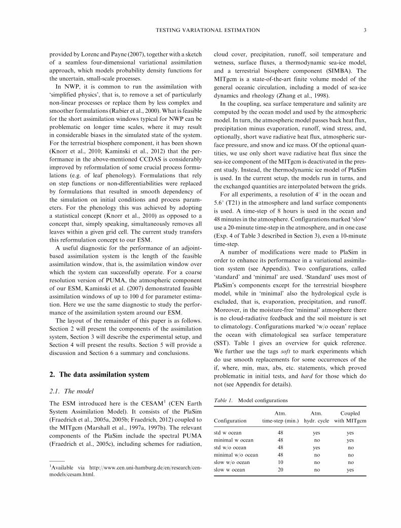
For all experiments, a resolution of 48 in the ocean and

5.68 (T21) in the atmosphere and land surface components

is used. A time-step of 8 hours is used in the ocean and

48minutes in the atmosphere. Configurations marked ‘slow’

use a 20-minute time-step in the atmosphere, and in one case

(Exp. 4 of Table 3 described in Section 3), even a 10-minute

time-step.

A number of modifications were made to PlaSim in

order to enhance its performance in a variational assimila-

tion system (see Appendix). Two configurations, called

‘standard’ and ‘minimal’ are used. ‘Standard’ uses most of

PlaSim’s components except for the terrestrial biosphere

model, while in ‘minimal’ also the hydrological cycle is

excluded, that is, evaporation, precipitation, and runoff.

Moreover, in the moisture-free ‘minimal’ atmosphere there

is no cloud-radiative feedback and the soil moisture is set

to climatology. Configurations marked ‘w/o ocean’ replace

the ocean with climatological sea surface temperature

(SST). Table 1 gives an overview for quick reference.

We further use the tags soft to mark experiments which

do use smooth replacements for some occurrences of the

if, where, min, max, abs, etc. statements, which proved

problematic in initial tests, and hard for those which do

not (see Appendix for details).

Table 1. Model configurations

Configuration

Atm.

time-step (min.)

Atm.

hydr. cycle

Coupled

with MITgcm

std w ocean 48 yes yes

minimal w ocean 48 no yes

std w/o ocean 48 yes no

minimal w/o ocean 48 no no

slow w/o ocean 10 no no

slow w ocean 20 no yes1Available via http://www.cen.uni-hamburg.de/en/research/cen-

models/cesam.html.

TESTING VARIATIONAL ESTIMATION 3

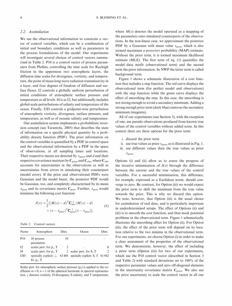
http://www.cen.uni-hamburg.de/en/research/cen-models/cesam.html

http://www.cen.uni-hamburg.de/en/research/cen-models/cesam.html

2.2. Assimilation

We use the observational information to constrain a vec-

tor of control variables, which can be a combination of

initial and boundary conditions as well as parameters in

the process formulations of the model. Our experiments

will investigate several choices of control vectors summa-

rised in Table 2. P10 is a control vector of process param-

eters from PlaSim, controlling the time scale for Rayleigh

friction in the uppermost two atmospheric layers, the

diffusion time scales for divergence, vorticity, and tempera-

ture, the point of mean long wave radiation transmissivity in

a layer, and four degrees of freedom of diffusion and sur-

face fluxes. I2 controls a globally uniform perturbation of

initial conditions of atmospheric surface pressure and

temperature at all levels. I4 is as I2, but additionally includes

global-scale perturbations of salinity and temperature of the

ocean. Finally, I3D controls a gridpoint-wise perturbation

of atmospheric vorticity, divergence, surface pressure, and

temperature, as well as of oceanic salinity and temperature.

Our assimilation system implements a probabilistic inver-

sion concept (see Tarantola, 2005) that describes the state

of information on a specific physical quantity by a prob-

ability density function (PDF). The prior information on

the control variables is quantified by a PDF in control space

and the observational information by a PDF in the space

of observations, at all sampling times and locations.

Their respective means are denoted by xprior and d and their

respective covariancematrices byCprior andCobs, whereCobs

accounts for uncertainties in the observations as well as

uncertainties from errors in simulating their counterpart

(model error). If the prior and observational PDFs were

Gaussian and the model linear, the posterior PDF would

be Gaussian, too, and completely characterised by its mean

xpost and its covariance matrix Cpost. Further, xpost would

minimise the following cost function:

JðxÞ ¼ 1

2½ðMðxÞ � dÞTCCC�1

obs:ðMðxÞ � dÞ

þ ðx� xpriorÞTCCC�1

priorðx� xpriorÞ�;(1)

where M(x) denotes the model operated as a mapping of

the parameters onto simulated counterparts of the observa-

tions. In the non-linear case, we approximate the posterior

PDF by a Gaussian with mean value xpost, which is also

termed maximum a posteriori probability (MAP) estimate.

Without the prior term, it is termed maximum likelihood

estimate (MLE). The first term of eq. (1) quantifies the

model�data misfit (observational term) and the second

term the prior information. In NWP the latter term is called

background term.

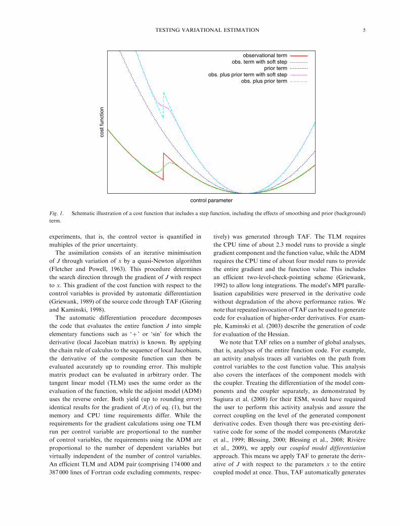
Figure 1 shows a schematic illustration of a cost func-

tion that includes a step function. The red curve displays the

observational term (for perfect model and observations)

with the step function while the green curve displays the

effect of smoothing the step. In this case, the smoothing is

not strong enough to avoid a secondary minimum. Adding a

strong enough prior term (dark blue) removes the secondary

minimum (magenta).

All of our experiments (see Section 3), with the exception

of one, use pseudo observations produced from known true

values of the control variables without added noise. In this

context there are three options for the prior term:

i. discard the prior term

ii. use true values as prior xprior as is illustrated in Fig. 1.

iii. use different values than the true values as prior

xprior

Options (i) and (ii) allow us to assess the progress of

the iterative minimisation of J(x) through the difference

between the current and the true values of the control

variables. For a successful minimisation, this difference,

for example, expressed as a Euclidean norm, should con-

verge to zero. By contrast, for Option (iii) we would expect

the prior term to shift the minimum from the true value

towards the prior. This is why we discard this option.

We note, however, that Option (iii) is the usual choice

for assimilation of real data, and is particularly important

in underdetermined setups. The effect of Options (ii) and

(iii) is to smooth the cost function, and thus mask potential

problems in the observational term. Figure 1 schematically

illustrates the smoothing effect for Option (ii). For Option

(iii), the effect of the prior term will depend on its loca-

tion relative to the two minima in the observational term.

For our experiments, we choose Option (i) in order to make

a clear assessment of the properties of the observational

term. We demonstrate, however, the effect of including

a prior term (Option (ii)) for two of our experiments,

which use the P10 control vector (described in Section 3

and Table 2) with standard deviations set to 100% of the

respective parameter values and zero off-diagonal elements

in the uncertainty covariance matrix Cprior. We also use

the prior uncertainty to scale the control vector in all our

Table 2. Control vectors

Name Atmosphere Dim. Ocean Dim.

P10 10 process

parameters

10 � �

I2 scalar pert. for ps, T 2 � 0

I4 scalar pert. for ps, T 2 scalar pert. for S, T 2

I3D spatially explicit: z,

D, ps, T

63 488 spatially explicit: S, T 61 942

Scalar pert. for atmospheric surface pressure (ps) is applied to the co-

efficient m�0, n�1 of the spherical harmonic in spectral representa-

tion. z denotes vorticity, D divergence, S salinity, and T temperature.


experiments, that is, the control vector is quantified in

multiples of the prior uncertainty.

The assimilation consists of an iterative minimisation

of J through variation of x by a quasi-Newton algorithm

(Fletcher and Powell, 1963). This procedure determines

the search direction through the gradient of J with respect

to x. This gradient of the cost function with respect to the

control variables is provided by automatic differentiation

(Griewank, 1989) of the source code through TAF (Giering

and Kaminski, 1998).

The automatic differentiation procedure decomposes

the code that evaluates the entire function J into simple

elementary functions such as ‘�’ or ‘sin’ for which the

derivative (local Jacobian matrix) is known. By applying

the chain rule of calculus to the sequence of local Jacobians,

the derivative of the composite function can then be

evaluated accurately up to rounding error. This multiple

matrix product can be evaluated in arbitrary order. The

tangent linear model (TLM) uses the same order as the

evaluation of the function, while the adjoint model (ADM)

uses the reverse order. Both yield (up to rounding error)

identical results for the gradient of J(x) of eq. (1), but the

memory and CPU time requirements differ. While the

requirements for the gradient calculations using one TLM

run per control variable are proportional to the number

of control variables, the requirements using the ADM are

proportional to the number of dependent variables but

virtually independent of the number of control variables.

An efficient TLM and ADM pair (comprising 174 000 and

387 000 lines of Fortran code excluding comments, respec-

tively) was generated through TAF. The TLM requires

the CPU time of about 2.3 model runs to provide a single

gradient component and the function value, while the ADM

requires the CPU time of about four model runs to provide

the entire gradient and the function value. This includes

an efficient two-level-check-pointing scheme (Griewank,

1992) to allow long integrations. The model’s MPI paralle-

lisation capabilities were preserved in the derivative code

without degradation of the above performance ratios. We

note that repeated invocation of TAFcanbe used to generate

code for evaluation of higher-order derivatives. For exam-

ple, Kaminski et al. (2003) describe the generation of code

for evaluation of the Hessian.

We note that TAF relies on a number of global analyses,

that is, analyses of the entire function code. For example,

an activity analysis traces all variables on the path from

control variables to the cost function value. This analysis

also covers the interfaces of the component models with

the coupler. Treating the differentiation of the model com-

ponents and the coupler separately, as demonstrated by

Sugiura et al. (2008) for their ESM, would have required

the user to perform this activity analysis and assure the

correct coupling on the level of the generated component

derivative codes. Even though there was pre-existing deri-

vative code for some of the model components (Marotzke

et al., 1999; Blessing, 2000; Blessing et al., 2008; Riviere

et al., 2009), we apply our coupled model differentiation

approach. This means we apply TAF to generate the deriv-

ative of J with respect to the parameters x to the entire

coupled model at once. Thus, TAF automatically generates

cost

func

tion

control parameter

observational termobs. term with soft step

prior termobs. plus prior term with soft step

obs. plus prior term

Fig. 1. Schematic illustration of a cost function that includes a step function, including the effects of smoothing and prior (background)

term.


a single derivative code for all coupled model components,

including the coupler. No further hand-coding is required,

that is, for the reasons given, safer, more flexible and

sustainable. In the context of this study, it allowed us

to generate derivative code versions for a variety of com-

binations of model configurations, control vectors, and

observational data sets.

2.3. Data sets for assimilation

‘Identical twin’ experiments use pseudo-data in the assim-

ilation, which were generated with the model itself from a

prescribed control vector, thus guaranteeing full consistency

of data and model, and allowing us to know the ‘true’

control vector. For one other experiment, data interpolated

from ERA-40 simulations (Uppala et al., 2005) are used

in the atmosphere. In either case, data are provided at all

grid points and levels of the respective subsystem, with

the exception of atmospheric temperature at the upper-

most level. For the atmosphere we are using vorticity,

temperature, and surface pressure, while in the ocean these

are temperature and salinity. As in Kohl and Willebrand

(2002), all data are time-averaged over the assimilation

window and no noise is added. Consequently, the cost

function is evaluated at the end of the assimilation window.

Given the spatial resolution of T21 and 10 levels in the

atmosphere and 48 and 15 levels in the ocean, this amounts

to 40 960 time-averaged observations from the atmosphere

and (restricting to wet points) 61 942 from the ocean,

totalling 102 902.

For Cobs of eq. (1), off-diagonal elements where set

to zero, that is, we assume uncorrelated uncertainty. The

diagonal elements are the squares of the following standard

deviations: In the atmosphere we use 3 K for temperature,

5 hPa for surface pressure, and 2�105 1/s for vorticity.

Our ocean uncertainties vary in space with standard

deviations of 0.4�3.1 K for temperature and 0.15�0.8PSU for salinity with the higher values towards the surface.

These numbers are a rough guess of the actual uncertainties

and effectively determine the relative weight given to the

individual observation.

3. Experimental setup

Our experiments are designed to verify the correctness of

the derivatives and to identify potential problems under a

variety of situations. They present the first steps towards

an assimilation system in a coupled model environment.

We will examine several combinations of model configura-

tions and control vectors.

For each of the model configurations, we generate a

consistent snapshot of the model state (restart file) recorded

at the end of a 10-yr integration. The restart file for the

experiment with the ERA-40 data is derived by optimis-

ing the atmospheric initial conditions in a pre-assimilation

over 200 iterations. This procedure uses as additional term

in eq. (1), a surface pressure tendency penalty to suppress

gravity waves as given in eq. 2.4 of Zou et al. (1993),

summed over all time steps during the first 6 hours of a 1-d

assimilation window, while the observational constraint

was constructed as the time-averaged data over the full

assimilation window. All but the aforementioned experi-

ment will be conducted as identical twin experiments that

assimilate pseudo data. This means we use default values

of the control vector to generate pseudo data. Next, we

start the iterative assimilation procedure from a perturbed

control vector. For the identical twin experiments with

short control vectors, that is, P10, I2, I4 as defined in

Table 2, we call an experiment successful if we can

accurately (Euclidean distance to default reduced by at least

five orders of magnitude) recover the default parameter

values through assimilation of the data, with a strongly

(by more than five orders of magnitude) reduced gradient

of the cost function.

Now, in the most favourable case of a linear model, we

can expect a solution of this type of inverse problem to take

as many iterations as there are components in the control

vector (Powell, 1964). Since for an ESM one can usually

only afford an iteration number of a few tens or hundreds,

we can only expect setups with low dimensional control

vectors to converge. For the setups with high-dimensional

control vector, that is, I3D, we will only perform 20

iterations. In this context, we call an experiment successful,

if reductions of the cost function and of the Euclidean

distance of the control vector to the default values are

achieved at the same time. In an apparently underdeter-

mined setup such as I3D (with 125 430 control variables

constrained by 102 902 observations) the improvement of

the control vector is of particular importance.

Within the iterative minimisation, the trajectory of the

control vector through the control space is highly depen-

dent on the initial parameter vector. This means that two

minimisations starting from neighbouring control vectors

typically explore quite different regions in control space even

if they converge to the same minimum. For an example,

see Fig. 4 in Clerici et al. (2010). To assess the robustness

of our experimental results, we carry out each experiment

as a small ensemble with four members, each of which

starts from a different point in control space. For the

identical twin experiments with the I4 control vector the

first member starts with the following perturbations of

the control vector: in atmosphere and ocean 0.1 K for

temperature, 1 per mil of the atmospheric surface pressure,

0.1 PSU for salinity. For the other members, the same

magnitudes are used, but with varied signs. For example

in the ‘min w ocean’ configuration this uniform initial


state perturbation yields, after a 26 d integration, a per-

turbation of about 1.5 K in the lowest atmospheric layer

(standard deviation), with maximum values of 18 K and

10 hPa. For the P10 control vector, a 10% perturbation

of each component is used. The I3D control vector uses

a globally uniform perturbation of the same magnitude

as in the I4 case, but sign and magnitude are varied to

generate the other ensemble members. An ensemble size of

four is low, but appears to be sufficient for a first assessment.

4. Results

First we address model parameter estimation, that is, the

control vector P10, in a set of identical twin experiments.

Table 3 summarises our experimental results. Exp. 1 shows

that in the most complex configuration ‘std w ocean’, we

cannot even reliably recover our parameter vector over a 1-d

assimilation window. Three out of four ensemble members

fail to find a minimum. The minimisations get stuck at edges

in the cost function. This is because, with a given minimal

step size along a local downhill direction that is pointing

towards an upward jump, the optimisation algorithm

cannot achieve any further decrease of the cost function.

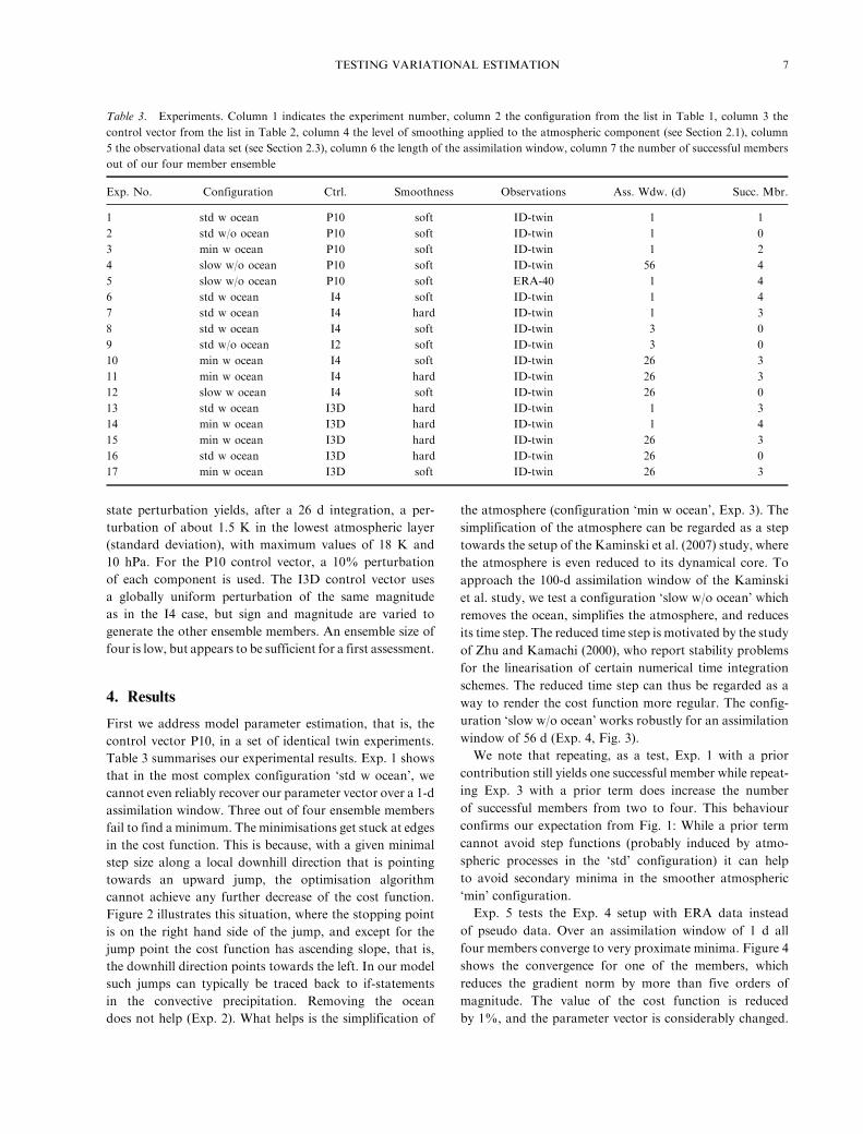
Figure 2 illustrates this situation, where the stopping point

is on the right hand side of the jump, and except for the

jump point the cost function has ascending slope, that is,

the downhill direction points towards the left. In our model

such jumps can typically be traced back to if-statements

in the convective precipitation. Removing the ocean

does not help (Exp. 2). What helps is the simplification of

the atmosphere (configuration ‘min w ocean’, Exp. 3). The

simplification of the atmosphere can be regarded as a step

towards the setup of the Kaminski et al. (2007) study, where

the atmosphere is even reduced to its dynamical core. To

approach the 100-d assimilation window of the Kaminski

et al. study, we test a configuration ‘slow w/o ocean’ which

removes the ocean, simplifies the atmosphere, and reduces

its time step. The reduced time step is motivated by the study

of Zhu and Kamachi (2000), who report stability problems

for the linearisation of certain numerical time integration

schemes. The reduced time step can thus be regarded as a

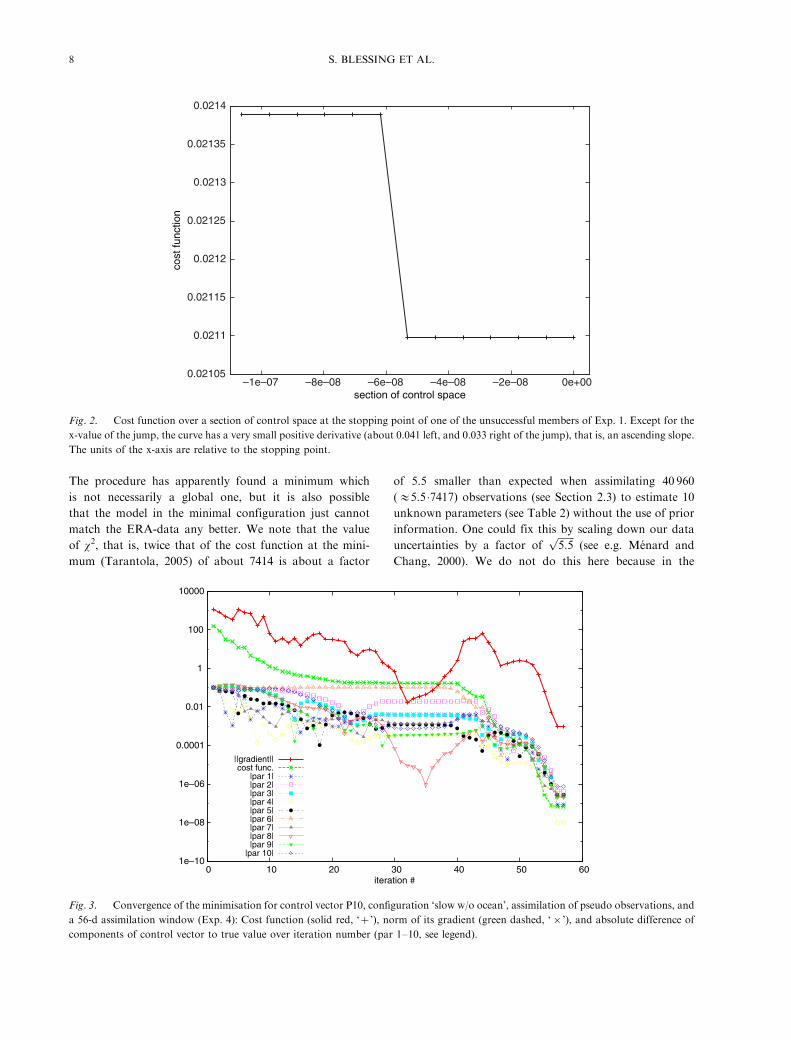
way to render the cost function more regular. The config-

uration ‘slow w/o ocean’ works robustly for an assimilation

window of 56 d (Exp. 4, Fig. 3).

We note that repeating, as a test, Exp. 1 with a prior

contribution still yields one successful member while repeat-

ing Exp. 3 with a prior term does increase the number

of successful members from two to four. This behaviour

confirms our expectation from Fig. 1: While a prior term

cannot avoid step functions (probably induced by atmo-

spheric processes in the ‘std’ configuration) it can help

to avoid secondary minima in the smoother atmospheric

‘min’ configuration.

Exp. 5 tests the Exp. 4 setup with ERA data instead

of pseudo data. Over an assimilation window of 1 d all

four members converge to very proximate minima. Figure 4

shows the convergence for one of the members, which

reduces the gradient norm by more than five orders of

magnitude. The value of the cost function is reduced

by 1%, and the parameter vector is considerably changed.

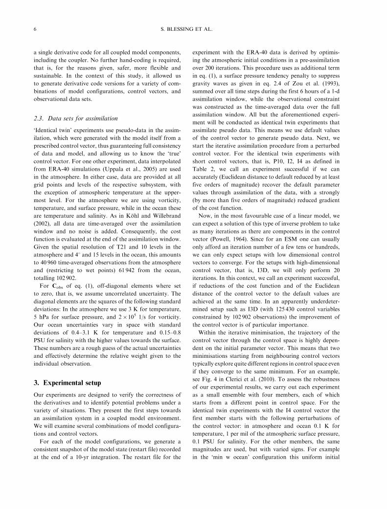
Table 3. Experiments. Column 1 indicates the experiment number, column 2 the configuration from the list in Table 1, column 3 the

control vector from the list in Table 2, column 4 the level of smoothing applied to the atmospheric component (see Section 2.1), column

5 the observational data set (see Section 2.3), column 6 the length of the assimilation window, column 7 the number of successful members

out of our four member ensemble

Exp. No. Configuration Ctrl. Smoothness Observations Ass. Wdw. (d) Succ. Mbr.

1 std w ocean P10 soft ID-twin 1 1

2 std w/o ocean P10 soft ID-twin 1 0

3 min w ocean P10 soft ID-twin 1 2

4 slow w/o ocean P10 soft ID-twin 56 4

5 slow w/o ocean P10 soft ERA-40 1 4

6 std w ocean I4 soft ID-twin 1 4

7 std w ocean I4 hard ID-twin 1 3

8 std w ocean I4 soft ID-twin 3 0

9 std w/o ocean I2 soft ID-twin 3 0

10 min w ocean I4 soft ID-twin 26 3

11 min w ocean I4 hard ID-twin 26 3

12 slow w ocean I4 soft ID-twin 26 0

13 std w ocean I3D hard ID-twin 1 3

14 min w ocean I3D hard ID-twin 1 4

15 min w ocean I3D hard ID-twin 26 3

16 std w ocean I3D hard ID-twin 26 0

17 min w ocean I3D soft ID-twin 26 3


The procedure has apparently found a minimum which

is not necessarily a global one, but it is also possible

that the model in the minimal configuration just cannot

match the ERA-data any better. We note that the value

of x2, that is, twice that of the cost function at the mini-

mum (Tarantola, 2005) of about 7414 is about a factor

of 5.5 smaller than expected when assimilating 40 960

(:5.5 �7417) observations (see Section 2.3) to estimate 10

unknown parameters (see Table 2) without the use of prior

information. One could fix this by scaling down our data

uncertainties by a factor offfiffiffiffiffiffiffi

5:5p

(see e.g. Menard and

Chang, 2000). We do not do this here because in the

0.02105

0.0211

0.02115

0.0212

0.02125

0.0213

0.02135

0.0214

–1e–07 –8e–08 –6e–08 –4e–08 –2e–08 0e+00

cost

func

tion

section of control space

Fig. 2. Cost function over a section of control space at the stopping point of one of the unsuccessful members of Exp. 1. Except for the

x-value of the jump, the curve has a very small positive derivative (about 0.041 left, and 0.033 right of the jump), that is, an ascending slope.

The units of the x-axis are relative to the stopping point.

1e–10

1e–08

1e–06

0.0001

0.01

1

100

10000

0 10 20 30 40 50 60iteration #

||gradient||cost func.

|par 1||par 2||par 3||par 4||par 5||par 6||par 7||par 8||par 9|

|par 10|

Fig. 3. Convergence of the minimisation for control vector P10, configuration ‘slow w/o ocean’, assimilation of pseudo observations, and

a 56-d assimilation window (Exp. 4): Cost function (solid red, ‘�’), norm of its gradient (green dashed, ‘�’), and absolute difference of

components of control vector to true value over iteration number (par 1�10, see legend).


absence of a prior term a uniform scalar has no impact

on the minimisation. Figure 5 shows that the estimated

parameter vector achieves a slight improvement of the

predictive skill beyond the assimilation window.

Next, we present experiments where we estimate initial

conditions (control vectors I2, I4, and I3D). We start with

the most complex configuration, ‘std w ocean’, and the I4

control vector, which works for assimilation windows of

1 d with (Exp. 6) and mostly without (Exp. 7) soft switches.

For a 3-d assimilation window, the assimilation does not

work anymore (Exp. 8). Removing the ocean (Exp. 9) does

not help. We can, however, achieve considerable extensions

of the assimilation window if we simplify the atmospheric

component. Configuration ‘min w ocean’ is mostly success-

ful for an assimilation window of 26 d with (Exp. 10) and

without (Exp. 11, Fig. 6) soft switches. Interestingly, reduc-

ing the time step deteriorates the estimation of initial con-

ditions (Exp. 12), even though it improved the estimation

1.4

1.6

1.8

2

2.2

2.4

2.6

0 0.5 1 1.5 2

RM

S-e

rror

of a

tmos

pher

ic te

mpe

ratu

res

[K]

integration time [d]

prior-datapost-data

Fig. 5. RMS of temperature difference during and after assimilation window for Exp. 5.

1e–041e–031e–021e–011e+001e+011e+02

||gradient||

3700

3710

3720

3730

3740

3750cost func.

0

1

2

3

4

5

6

0 50 100 150 200 250

iteration #

||parameter||

Fig. 4. Convergence of the minimisation for control vector P10, configuration ‘slow w/o ocean’, assimilation of ERA observations, and a

1-d assimilation window (Exp. 5): Norm of its gradient (top), cost function (centre), and absolute difference of the components of the

control vector to the default value (labelled ‘true’ value in ID-twin experiments, bottom) over iteration number.


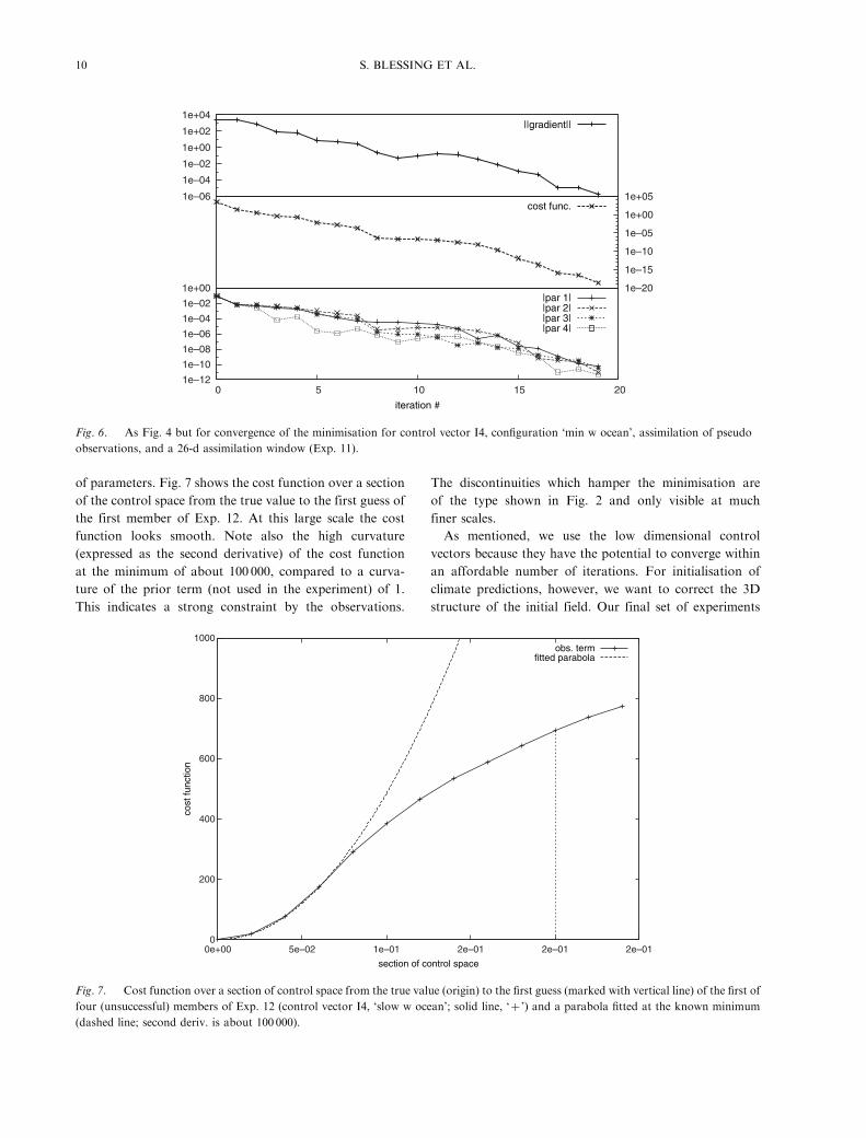
of parameters. Fig. 7 shows the cost function over a section

of the control space from the true value to the first guess of

the first member of Exp. 12. At this large scale the cost

function looks smooth. Note also the high curvature

(expressed as the second derivative) of the cost function

at the minimum of about 100 000, compared to a curva-

ture of the prior term (not used in the experiment) of 1.

This indicates a strong constraint by the observations.

The discontinuities which hamper the minimisation are

of the type shown in Fig. 2 and only visible at much

finer scales.

As mentioned, we use the low dimensional control

vectors because they have the potential to converge within

an affordable number of iterations. For initialisation of

climate predictions, however, we want to correct the 3D

structure of the initial field. Our final set of experiments

0

200

400

600

800

1000

0e+00 5e–02 1e–01 2e–01 2e–01 2e–01

cost

func

tion

section of control space

obs. termfitted parabola

Fig. 7. Cost function over a section of control space from the true value (origin) to the first guess (marked with vertical line) of the first of

four (unsuccessful) members of Exp. 12 (control vector I4, ‘slow w ocean’; solid line, ‘�’) and a parabola fitted at the known minimum

(dashed line; second deriv. is about 100 000).

1e–06

1e–04

1e–02

1e+00

1e+02

1e+04||gradient||

1e–20

1e–15

1e–10

1e–05

1e+00

1e+05cost func.

1e–12

1e–10

1e–08

1e–06

1e–04

1e–02

1e+00

0 5 10 15 20

iteration #

|par 1||par 2||par 3||par 4|

Fig. 6. As Fig. 4 but for convergence of the minimisation for control vector I4, configuration ‘min w ocean’, assimilation of pseudo

observations, and a 26-d assimilation window (Exp. 11).


tests this type of control vector (I3D) and limits the number

of iterations of our gradient algorithm to 20. Recall that in

this context we call an experiment successful, if reductions

of the cost function and of the Euclidean distance of the

control vector to the default values are achieved at the same

time. Over 1 d, our most complex configuration ‘std w

ocean’ (Exp. 13) has three successful ensemble members

(9, 13, and 14% reduction of norm of parameter difference

to truth and cost function reductions of 32, 20, and 19%),

while one member got stuck without reduction in the

norm of the parameter difference to truth nor in the cost

function. By contrast, over the same assimilation window

in configuration ‘min w ocean’ (Exp. 14) all four ensemble

members are successful, with 11, 12, 15, and 15% reduction

of norm of parameter difference to truth and cost function

reductions of 34, 20, 30, and 20%. In this latter configura-

tion, three ensemble members were also successful for an

assimilation window of 26 d (Exp. 15, Fig. 8) with 2, 5, and

10% reduction of norm of parameter difference to truth

and cost function reductions of 10, 17, and 20%, while the

same assimilation fails for the configuration ‘std w ocean’

(Exp. 16). Running the configuration ‘min w ocean’ with

soft switches (Exp. 17) again yields three successful

ensemble members with comparable results (parameter

vector: 5, 7, and 10% reduction; cost function: 25, 14,

and 28% reduction).

5. Discussion

Running the uncoupled atmospheric model does not yield

results superior to the coupled one, as we see in Exp. 2/1

and Exp. 9/8. This reflects the fact that the processes in the

ocean model operate on longer time scales than those in the

atmospheric model. In particular, switching off fast atmo-

spheric processes such as precipitation increases the feasible

assimilation window. The non-linear behaviour of these

processes is aggravated by their numerical implementation,

which often incorporates non-differentiable statements.

A step function, for example, produces discontinuities in

the cost function, which may provide an obstacle for

gradient-based minimisation. In this study, the replacement

of some of these formulations by differentiable approxima-

tions in the soft experiments has been limited to just a few

parts in PlaSim. Hence, we expect future studies to reveal

the full potential that lies in the reformulation of such

processes in a differentiable way, possibly using statistical

concepts as demonstrated by (Knorr et al., 2010) and

(Kaminski et al., 2012).

The size of the time-step in dynamical models is typically

a trade-off between performance and simulation quality.

A long time-step results in a fast model integration, while

a short time step typically reduces discretisation error and

thus enhances the quality of the simulation. Exceeding

a certain threshold (imposed by the CFL criterion) even

results in an unstable integration. In our experiments,

a reduction of the atmospheric time step improves the

performance for parameter estimation (Exp. 4) but dete-

riorates it for the estimation of the initial state (Exp. 12).

An obvious qualitative difference between parameter and

initial state estimation is that model parameters directly

influence the cost function at each time-step throughout

the integration, while the influence of the initial state is

indirect, because it has to be propagated from time step to

time step through the integration of the dynamical system.

1e+01

1e+02

1e+03

1e+04||gradient||

4.5e+02

5.0e+02

5.5e+02

6.0e+02cost func.

38

39

40

41

42

43

0 5 10 15 20iteration #

||parameter||

Fig. 8. As Fig. 4 but for convergence of the minimisation for control vector I3D, configuration ‘min w ocean’, assimilation of pseudo

observations, and a 26-d assimilation window (Exp. 15).


This propagation has the potential to dampen or compli-

cate the structure of the sensitivity of the cost function to

an initial state change. Our experiments may show the

balance of two mechanisms with opposite effect. On one

hand a reduced time step enhances stability of the line-

arised model (Zhu and Kamachi, 2000), but on the other

hand it increases the number of time steps required to cover

a given assimilation window. It may be that the first mech-

anism is dominant for parameter estimation while the

second mechanism is dominant for the estimation of initial

conditions. To confirm these findings further research is

required, including theoretical studies with simple models.

Assimilation of ERA-data in Exp. 5 certainly is more

challenging than the identical twin experiments. Even

though we used an assimilation procedure to prepare the

initial state for the experiment, it is obvious from the

RMS error growth in Fig. 5 that the model trajectory

quickly diverges from the data. Still it is possible to

improve this situation slightly by the parameter estimation.

The difficulty lies in a combination of four factors: First,

the atmospheric configuration is simplified. Second, the

model resolution is coarse compared to the data source.

Third, despite the pre-assimilation procedure the initial

state is still sub-optimal. Fourth, the P10 control space

is small. We can eliminate the first two of these factors

by repeating the same procedure with the ERA data

replaced by observations generated by the model from

initial conditions of a different year. In this case the cost

function reduction is stronger by a factor of more than 10.

This indicates the potential for a more realistic model

and higher resolution.

6. Summary and conclusions

We demonstrated a coupled model differentiation approach

that applies, for the first time, automatic differentiation

to an entire ESM at once. The generated derivative code is

efficient and easy to maintain and to adapt to changes in

the ESM code. No hand-coding is required at the deriva-

tive level. We further constructed a variational assimilation

system around the ESM and demonstrated the assimilation

of pseudo observations as well as of an atmospheric data

set based on ERA, and addressed estimation of process

parameters and initial conditions. For both applications,

using pseudo and ERA data, we quantify the performance

of the assimilation system by the length of the feasible

assimilation window.

The focus of this study lies on the behaviour of the adjoint

ESM in a standard assimilation environment, rather than

on the construction of a sophisticated assimilation system,

for example, with split in inner and outer optimisation

loops (see e.g. Rabier et al., 2000). We also refrained

from using a prior (or background) term in the cost function

(eq. 1) in our experiments (except for a demonstration)

in order to make a clearer assessment of the constraints

on the coupled model provided by the observational term.

Through its parabolic contribution to the cost function,

a prior term would have stabilised the inverse problem.

This would have clearly facilitated the minimisation and

possibly would have masked convergence problems im-

posed by the observational term. In that respect we can

regard our assessment as conservative.

We find that the performance of the coupled model in

the assimilation system is highly dependent on the selec-

tion of atmospheric processes and their implementation.

A reduced atmospheric configuration with a number of

processes deactivated shows significantly better perfor-

mance than the standard configuration, while inclusion or

exclusion of the dynamical ocean component has only

a minor effect. Reducing the atmospheric time-step helps

the estimation of process parameters but complicates the

estimation of initial conditions. We note that the absolute

performance of the system is likely to change with the

resolution of the model. For example, we would expect a

degraded performance for enhanced resolution of the ocean

or atmosphere component or both. Nevertheless, the above

findings should hold over a range of resolutions, because

the responsible mechanisms are resolution-independent.

The performance in the reduced configuration is much

better when estimating parameters by assimilating pseudo

data generated by the model itself instead of by assimilating

ERA data, in spite of careful preparation of the initial

conditions. Part of this difference may be attributed to the

coarse resolution and a too large degree of simplification in

the reduced configuration with a limited number of control

variables. More work is required to improve the balance

between realistic process representations and good perfor-

mance in the assimilation system. The efficient handling

of longer control vectors was demonstrated in the present

study. Another perspective to further extend the feasible

assimilation window is the combined use of a reduced

and full configuration in a variational assimilation system,

where the reduced configuration is used to provide an

approximate gradient.

The study presented a first step towards a flexible

variational assimilation system for initialisation of predic-

tions and calibration of the ESM against observations. The

system was demonstrated in an idealised set up. Obvious

next steps are an increase of spatio-temporal resolution,

extension/improvement of the process representations in a

differentiable form, and the simultaneous use of observa-

tions of the entire climate system. A further obvious appli-

cation is sensitivity studies based on the tangent and adjoint

ESM. The TAF compliance of the system assures fast

updates after any modification of the ESM code.


7. Acknowledgements

This work was supported by the European Community

within the 6th Framework Programme for Research and

Technological Development under contract no. 212643

(THOR) to Hamburg University and supported in part

also through the DFG funded CLISAP excellence initiative.

The presented research is building on work on an assimila-

tion system developed around only PlaSim that was funded

by NERC through its QUEST programme. M. Scholze

contributed through that phase and acknowledges support

through a CLISAP fellowship. P. Herrmann was supported

through a Max-Planck Fellow Grant to D. Stammer.

The authors wish to thank E. Kirk for his advice throughout

this study and valuable comments on the manuscript.

8. Appendix

Based on a set of initial tests with PlaSim, we identified

several spots in the process implementations that produced

a non-smooth shape in the cost function. For these spots we

modified the implementation. Even though these modifica-

tions are specific to the model at hand, it is instructive to

give a few examples.

(1) if- and where- statements which depend on the

model state implement piecewise-defined functions.

Especially in the boundary-layer parameterisation of

the PlaSim it was possible to make these functions

smooth and differentiable at the switching point by

readjusting some of their coefficients.

(2) In some places of the PlaSim, the above procedure

was infeasible and one of the branches was selected

and the other removed. Alternatively, an approach

was used which gives a weighted combination of the

results of both branches, using a sigmoid function

depending on the if-condition.

(3) The PlaSim does its time stepping in spectral space

and has to deal with spurious negative moisture stem-

ming from the Fourier-transform. The original model

uses a redistribution algorithmwhich fills up negative

moisture at affected grid cells, taking it from a certain

domain. Out of vertical column containing the

affected grid cell, latitude band, and global domain,

it chooses the smallest domain that contains enough

moisture. Switching this off had a positive effect on

the smoothness of the cost function at the expense of

formal moisture conservation. Given the limited

assimilation window, we do not expect a strong

detrimental effect for an assimilation. However,

simulations including atmospheric moisture require

a closed hydrological cycle, for example, rain, which is

currently implemented in a form far from smooth.

(4) In the PlaSim some of the min, max, and abs

statements were replaced by smooth approximations.

We note that the smoothing effect of the above modifica-

tions is limited, because, unlike Knorr et al. (2010), in

this initial study we refrained from redevelopment of entire

process representations (such as convection) in smooth

form.

References

Abarbanel, H., Kostuk, M. and Whartenby, W. 2010. Data

assimilation with regularized nonlinear instabilities. Q. J. Roy.

Meteorol. Soc. 136(648), 769�783. DOI: 10.1002/qj.600.

Blessing, S. 2000. Development and applications of an adjoint GCM.

Master’s Thesis. University of Hamburg, Germany.

Blessing, S., Fraedrich, K. and Lunkeit, F. 2004, Climate diagnostics

by adjoint modelling: a feasibility study. In: The KIHZ

Project: Towards a Synthesis of Holocene Proxy Data and Climate

Models (eds. H. Fischer, T. Kumke, G. Lohmann, G. Floser, H.,

H. von Storch and co-authors). Springer, Heidelberg, pp.

383�396.Blessing, S., Greatbatch, R., Fraedrich, K. and Lunkeit, F. 2008.

Interpreting the atmospheric circulation trend during the last

half of the twentieth century: application of an adjoint model.

J. Clim. 21, 4629�4646. DOI: 10.1175/2007JCLI1990.1.

Clerici, M., Voßbeck, M., Pinty, B., Kaminski, T., Taberner, M.

and co-authors. 2010. Consolidating the two-stream inversion

package (JRC-TIP). IEEE J. Sel. Top. Appl. Earth Obs. Remote

Sens. 3(3), 286�295. DOI: 10.1109/JSTARS.2010.2046626.

Cubasch, U., Meehl, G., Boer, G., Stouffer, R., Dix, M. and co-

authors. 2001, Projections of future climate change. In: Climate

Change 2001: The Scientific Basis (eds. J. T. Houghton, Y. Ding,

D. J. Griggs, M. Noguer, P. J. van der Linden, and co-authors).

Cambridge University Press, Cambridge, UK, chapter 9, pp.

525�582.Fletcher, R. and Powell, M. 1963. A rapidly convergent descent

method for minimization. Comput J. 6(2), 163�168.Fraedrich, K. 2012. A suite of user-friendly global climate models:

hysteresis experiments. Eur. Phys. J. Plus. 127(5), 53, 9 pp. DOI:

10.1140/epjp/i2012-12053-7.

Fraedrich, K., Jansen, H., Kirk, E., Luksch, U. and Lunkeit, F.

2005a. The planet simulator: towards a user friendly model.

Meteorol. Z. 14, 299�304.Fraedrich, K., Jansen, H., Kirk, E. and Lunkeit, F. 2005b.

The planet simulator: green planet and desert world. Meteorol.

Z. 14(3), 305�314.Fraedrich, K., Kirk, E., Luksch, U. and Lunkeit, F. 2005c.

The portable university model of the atmosphere (PUMA):

storm track dynamics and low frequency variability. Meteorol.

Z. 14, 735�745.Galanti, E., Tziperman, E., Harrison, M., Rosati, A. and Sirkes, Z.

2003. A study of ENSO prediction using a hybrid coupled model

and the adjoint method for data assimilation. Mon. Weather

Rev. 131(11), 2748�2764.Giering, R. and Kaminski, T. 1998. Recipes for adjoint code

construction. ACM Trans. Math. Softw. 24(4), 437�474.


Griewank, A. 1989. On automatic differentiation. In: Mathematical

Programming: Recent Developments and Applications (eds. M. Iri

and K. Tanabe). Kluwer Academic Publishers, Dordrecht, pp.

83�108.Griewank, A. 1992. Achieving logarithmic growth of temporal and

spatial complexity in reverse automatic differentiation. Optim.

Methods Softw. 1, 35�54.Hoteit, I., Cornuelle, B., Kohl, A. and Stammer, D. 2005. Treating

strong adjoint sensitivities in tropical eddy-permitting varia-

tional data assimilation. Q. J. Roy. Meteorol. Soc. 131(613),

3659�3682. DOI: 10.1256/qj.05.97.

Jones, C., Gregory, J., Thorpe, R., Cox, P., Murphy, J. and

co-authors. 2005. Systematic optimisation and climate simula-

tion of FAMOUS, a fast version of HadCM3. Clim. Dynam.

25(2�3), 189�204. DOI: 10.1007/s00382-005-0027-2.

Kaminski, T., Blessing, S., Giering, R., Scholze, M. and Voßbeck,

M. 2007. Testing the use of adjoints for estimation of GCM

parameters on climate time-scales. Meteorol. Z. 16(6), 643�652.Kaminski, T., Giering, R., Scholze, M., Rayner, P. and Knorr, W.

2003. An example of an automatic differentiation-based modelling

system. In: Computational Science � ICCSA 2003, International

Conference Montreal, Canada, May 2003, Proceedings, Part II,

Vol. 2668 of Lecture Notes in Computer Science (eds. V. Kumar,

L. Gavrilova, C. J. K. Tan and P. L’Ecuyer). Springer, Berlin, pp.

95�104.Kaminski, T., Knorr, W., Scholze, M., Gobron, N., Pinty, B. and

co-authors. 2012. Consistent assimilation of MERIS FAPAR

and atmospheric CO2 into a terrestrial vegetation model and

interactive mission benefit analysis. Biogeosciences. 9(8), 3173�3184. DOI: 10.5194/bg-9-3173�2012.

Kaminski, T., Knorr, W., Schurmann, G., Scholze, M., Rayner,

P. J. and co-authors. 2013. The BETHY/JSBACH carbon

cycle data assimilation system: experiences and challenges. J.

Geophys. Res. 118(4), 1414�1426. DOI: 10.1002/jgrg.20118.

Kauker, F., Gerdes, R., Karcher, M., Kaminski, T., Giering, R.

and co-authors. 2010. June 2010 Sea Ice Outlook � AWI/

FastOpt/OASys, Sea Ice Outlook web page. Online at: http://

www.arcus.org/search/seaiceoutlook.

Kauker, F., Kaminski, T., Karcher, M., Giering, R., Gerdes, R. and

co-authors. 2009. Adjoint analysis of the 2007 all time arctic sea-

ice minimum. Geophys. Res. Lett. 36(L03707), 5 pp. DOI: 10.1029/

2008GL036323.

Knorr, W. and Heimann, M. 2001. Uncertainties in global

terrestrial biosphere modeling, 1. A comprehensive sensitivity

analysis with a new photosynthesis and energy balance scheme.

Global Biogeochem. Cycles. 15(1), 207�225. DOI: 10.1029/

1998GB001059.

Knorr, W., Kaminski, T., Scholze, M., Gobron, N., Pinty, B. and

co-authors. 2010. Carbon cycle data assimilation with a generic

phenology model. J. Geophys. Res. 115, G04017. DOI: 10.1029/

2009JG001119.

Kohl, A. and Stammer, D. 2008. Variability of the meridional

overturning in the north Atlantic from the 50-year GECCO state

estimation. J. Phys. Oceanogr. 38, 1913�1930. DOI: 10.1175/

2008JPO3775.1.

Kohl, A. and Willebrand, J. 2002. An adjoint method for the

assimilation of statistical characteristics into eddy-resolving

ocean models. Tellus A. 54(4), 406�425. DOI: 10.1034/j.1600-

0870.2002.01294.x.

Kuppel, S., Peylin, P., Chevallier, F., Bacour, C., Maignan, F. and

Richardson, A. D. 2012. Constraining a global ecosystem model

with multi-site eddy-covariance data. Biogeosci. Discuss. 9(3),

3317�3380. DOI: 10.5194/bgd-9-3317-2012.

Lea, D. J., Allen, M. R. and Haine, T. W. N. 2000. Sensitivity

analysis of the climate of a chaotic system. Tellus A. 52, 523�532. DOI: 10.1034/j.1600-0870.2000.01137.x.

Lee, T., Boulanger, J.-P., Foo, A., Fu, L.-L. and Giering, R. 2000.

Data assimilation into an intermediate coupled ocean�atmosphere model: application to the 1997�98 El Nino. J.

Geophys. Res. 105(C11), 26063�26088.Lorenc, A. C. and Payne, T. 2007. 4d-var and the butterfly

effect: statistical four-dimensional data assimilation for a wide

range of scales. Q. J. Roy. Meteorol. Soc. 133(624), 607�614.DOI: 10.1002/qj.36.

Lorenz, E. 1963. Deterministic nonperiodic flow. J. Atmos. Sci.

20(2), 130�141.Luke, C. M. 2011. Modelling Aspects of Land-Atmosphere

Interaction: Thermal Instability in Peatland Soils and Land

Parameter Estimation Through Data Assimilation. PhD Thesis.

University of Exeter, UK. Online at: http://hdl.handle.net/

10036/3229

Marotzke, J., Giering, R., Zhang, Q. K., Stammer, D., Hill, C. N.

and Lee, T. 1999. Construction of the adjoint MIT ocean general

circulation model and application to Atlantic heat transport

sensitivity. J. Geophys. Res. 104, 29529�29548. DOI: 10.1029/

1999JC900236.

Marshall, J., Adcroft, A., Hill, C., Perelman, L. and Heisey, C.

1997a. A finite-volume, incompressible Navier-Stokes model

for studies of the ocean on parallel computers. J. Geophys. Res.

102(C3), 5753�5766. DOI: 10.1029/96JC02775.

Marshall, J., Hill, C., Perelman, L. and Adcroft, A. 1997b.

Hydrostatic, quasi-hydrostatic, and nonhydrostatic ocean mod-

eling. J. Geophys. Res. 102(C3), 5733�5752. DOI: 10.1029/

96JC02776.

Menard, R. and Chang, L.-P. 2000. Assimilation of stratospheric

chemical tracer observations using a Kalman filter. Part II: x2-

validated results and analysis of variance and correlation

dynamics. Mon. Weather Rev. 128, 2672�2686.Murphy, J. M., Sexton, D. M. H., Barnett, D. N., Jones, G. S.,

Webb, M. J. and co-authors. 2004. Quantification of modelling

uncertainties in a large ensemble of climate change simulations.

Nature. 430, 768�772.Pires, C., Vautard, R. and Talagrand, O. 1996. On extending

the limits of variational assimilation in nonlinear chaotic

systems. Tellus A. 48, 69�121. DOI: 10.1034/j.1600-0870.1996.

00006.x.

Powell, M. 1964. An efficient method for finding the minimum

of a function of several variables without calculating derivatives.

Comput. J. 7(2), 155�162.Rabier, F., Jarvinen, H., Klinker, E., Mahfouf, J.-F. and

Simmons, A. 2000. The ECMWF operational implementation

of four-dimensional variational assimilation. Part I: experimen-

tal results with simplified physics. Q. J. Roy. Meteorol. Soc. 126,

1143�1170. DOI: 10.1002/qj.49712656415.


http://www.arcus.org/search/seaiceoutlook

http://www.arcus.org/search/seaiceoutlook

http://hdl.handle.net/10036/3229

http://hdl.handle.net/10036/3229

Rayner, P., Scholze, M., Knorr, W., Kaminski, T., Giering, R.

and co-authors. 2005. Two decades of terrestrial carbon

fluxes from a carbon cycle data assimilation system (CCDAS).

Global Biogeochem. Cycles. 19(GB2026), 20 pp. DOI: 10.1029/

2004GB002254.

Riviere, O., Lapeyre, G. and Talagrand, O. 2009. A novel

technique for nonlinear sensitivity analysis: application to moist

predictability. Q. J. Roy. Meteorol. Soc. 135(643), 1520�1537.DOI: 10.1002/qj.460.

Scholze, M., Kaminski, T., Rayner, P., Knorr, W. and Giering,

R. 2007. Propagating uncertainty through prognostic CCDAS

simulations. J. Geophys. Res. 112, 13 pp. DOI: 10.1029/

2007JD008642.

Schurmann, G. J., Kostler, C., Kaminski, T., Giering, R.,

Scholze, M. and co-authors. 2013. Assimilation of NEE and

CO2-concentrations into the land-surface scheme of the MPI

earth system model. EGU General Assembly Conference

Abstracts, Vol. 15 of EGU General Assembly Conference

Abstracts, p. 9052. Online at: http://adsabs.harvard.edu/abs/

2013EGUGA.15.9052S

Stammer, D., Wunsch, C., Giering, R., Eckert, C., Heimbach, P.

and co-authors. 2002. The global ocean circulation during

1992�1997, estimated from ocean observations and a general

circulation model. J. Geophys. Res. 107(C9), 1�27. DOI:

10.1029/2001JC000888.

Stammer, D., Wunsch, C., Giering, R., Eckert, C., Heimbach,

P. and co-authors. 2003. Volume, heat and freshwater transports

of the global ocean circulation 1992�1997, estimated from

a general circulation model constrained by WOCE data. J.

Geophys. Res. 108(C1), 23 pp. DOI: 10.1029/2001JC001115.

Sugiura, N., Awaji, T., Masuda, S., Mochizuki, T., Toyoda, T. and

co-authors. 2008. Development of a four-dimensional varia-

tional coupled data assimilation system for enhanced analysis

and prediction of seasonal to interannual climate variations. J.

Geophys. Res. 113(C10017), 21 pp. DOI: 10.1029/2008JC004741.

Swanson, K., Vautard, R. and Pires, C. 1998. Four-dimensional

variational assimilation and predictability in a quasi-geostrophic

model. Tellus A. 50, 369�390. DOI: 10.1034/j.1600-0870.1998.

t01-4-00001.x.

Tanguay, M., Bartello, P. and Gauthier, P. 1995. Four-dimen-

sional data assimilation with a wide range of scales. Tellus A. 47,

974�997. DOI: 10.1034/j.1600-0870.1995.00204.x.

Tarantola, A. 2005. Inverse Problem Theory and Methods for

Model Parameter Estimation Tarantola, A. SIAM, Philadelphia.

Thuburn, J. 2005. Climate sensitivities via a Fokker-Planck adjoint

approach. Q. J. Roy. Meteorol. Soc. 131(605), 73�92. DOI:

10.1256/qj.04.46.

Uppala, S. M., Kallberg, P. W., Simmons, A. J., Andrae, U.,

Bechtold, V. D. C. and co-authors. 2005. The ERA40 re-analysis.

Q. J. Roy. Meteorol. Soc. 131, 2961�3012. DOI: 10.1256/qj.

04.176.

Zhang, J., Hibler, W., Steele, M. and Rothrock, D. 1998.

Arctic ice-ocean modeling with and without climate restoring.

J. Phys. Oceanogr. 28(2), 191�217.Zhu, J. and Kamachi, M. 2000. The role of time step size

in numerical stability of tangent linear models. Mon. Weather

Rev. 128, 1562�1572.Zou, X., Navon, I. M. and Sela, J. G. 1993. Control of gravity

oscillations in variational data assimilation. Mon. Wea. Rev.

121(1), 272�289.


http://adsabs.harvard.edu/abs/2013EGUGA.15.9052S

http://adsabs.harvard.edu/abs/2013EGUGA.15.9052S

testing variational estimation of process parameters and

Documents