algorithm for signal parameters estimation based … · algorithm for signal parameters estimation...

Algorithm for signal parameters estimation based on the differential

samples

PREDRAG B. PETROVIĆ Faculty of Technical Sciences

University of Kragujevac Svetog Save 65, 32000 Čačak

SERBIA [email protected]

Abstract: - This paper is concerned with the estimation of amplitude and phase of an analog multi-harmonic signal based on a series of differential values of the signal. To this end, assuming the signal fundamental frequency is known before hand (i.e., estimated in an independent stage), a complexity-reduced scheme is proposed here. The reduction in complexity is achieved owing to completely new analytical and summarized expressions that enable a quick estimation at a low numerical error. The propose algorithm for the calculation of the unknown parameters requires O((2M)2) flops, while the straightforward solution of the obtained equations takes O((2M)3) flops, where M is number of harmonic coefficients. It is proved that the estimation performance of the proposed algorithm can attain Cramer-Rao lower bound (CRLB) for sufficiently high signal-to-noise ratios. It is applied in signal reconstruction, spectral estimation, system identification, as well as in other important signal processing problems. The paper investigates the errors related to the signal parameter estimation, and there is a computer simulation that demonstrates the accuracy of these algorithms.

Key-Words: - Band-limited signals; differential values; analytical solutions; signal reconstruction; simulation 1 Introduction Estimating the amplitude and phase of a signal accurately even when the frequencies contained in the signal are already known is very important in many areas [1-2]. These include the dual-tone multiple frequencies (DTMF) signal detection in digital communications, ECG sinusoidal interference cancellation, recovery of biomedical signals, and pitch detection in automated transcription. In power systems, estimation of the harmonic components is necessary to ensure the quality of power supply.

In signal processing, reconstruction usually means determination of an original continuous signal from a sequence of equally spaced samples. It is a well-known fact that any real signal which is transmitted along a channel-like form will have a finite bandwidth. As the result, the received signal's spectrum cannot contain any frequencies above a maximum value, fmax=Mf (f is the fundamental frequency). Consequently, M frequencies provide a specification of everything we know about the signal spectrum in terms of a d.c. level plus the amplitudes and phases of just— i.e. all the information we have about the spectrum can be specified by 2M +1 numbers. Many attempts have

been made in respect to application of sampling techniques supported by optimal methods of reconstruction of band-limited signals in the form of a Fourier series (trigonometric polynomials) [3-6].

In this paper, the application of differential processing (sampling) methods for periodic signal reconstruction is analyzed, as opposed to the method based on the integration of the input analogue signal [7], along with the problem of subsequent reconstruction of the processed signals. This kind of approach (integration) to the processing was also considered in [8], where the standard matrix inversion is used as the method for reconstruction, which requires very intensive numerical calculation. In [7] it was noticed that the ac signal integration method produces a regular matrix form in the derived system of equations, provided an adequate choice is made regarding the time parameters within which the integration is done; this makes it possible to have a much more efficient reconstruction procedure subsequently.

If the differential value (samples) were assumed to be measured without errors, the presented algorithm without any further modifications can be used for signal reconstruction of periodic band-limited signals, which is the situation that occurs in

WSEAS TRANSACTIONS on SIGNAL PROCESSING Predrag B. Petrović

E-ISSN: 2224-3488 263 Volume 10, 2014

simulation. In a real environment and when the measuring is performed in practice, the samples are measured with error. The sampled values that are obtained in practice may not be the exact values of the signal at sampling points, but only averages of the signal near these points [6]. In this case, the suggested algorithm must be modified, in order to be able to determine the best signal estimate, according to the criterion assumed, just like in [6], [8] or [9-12].

The approach in this paper is based on the use of the values that were obtained as result of the differential processing of the continual input signal, in precisely defined time periods. This kind of processing was done, as many times as was needed to enable the reconstruction of the multi-harmonic signal that is the subject of the processing operation. In this way, it is possible to obtain a specific form of the linear equations system. This system can be simply solved by using the derived analytical and summarized expressions. For estimation of amplitude and phase of complex ac signal algorithm requires O((2M)2) flops, while the straightforward solution of the obtained equations takes O((2M)3) flops. For this reason, the proposed method offers a significant improvement in computational efficiency over the standard reconstruction algorithms, at a lower numerical error.

Table 1: The nomenclature used in the following parts of the paper

Symbol Meaning

f fundamental frequency of processing signal

s(t)

band limited input analogue signal

M

the number of signal spectrum ac (harmonic) components

ADC

analogue to digital converter

ak

the amplitude of the kth harmonic

k

the number of the harmonic

ψk

the phase angle of the kth harmonic

Unlike the IEEE standard that was analysed in [13], the algorithm proposed in this paper is significantly more stable and free of the propagation error. Namely, when using the procedure prescribed by the standard, the amplitude errors of the fundamental will propagate through the method since the amplitudes are used to reconstruct the

detected sine wave and obtain the results before they are used to determine the next harmonic parameters. Overall, the frequency and amplitude errors from the first calculation are propagated to the higher harmonics and the calculation of the nth harmonic will invariably be contaminated by the errors of the phases and amplitudes from previous steps. 2 Proposed Method for Processing Let us assume that the input signal of the fundamental frequency f is band limited to the first M harmonic components. This form of continuous signal with a complex harmonic content can be represented as a sum of the Fourier components as follows:

( ) ( )∑=

+=M

kkk ftkats

12sin ψπ (1)

By differentiating the signal (1) and by forming a system of equations of the same form, in order to determine the 2M unknowns (amplitudes and phases of the M harmonic), we get:

( )( ) ( )( )

( ) ( )

( ) ( ) ( ) ( )[ ]∑

∑

∑

=

=

=

=

−=

+=

⇒=

+

=

M

kklklk

M

kklkl

ltt

M

kkk

ftkftkfka

ftkfkatx

txdt

ftkad

dttsd

l

1

1

1

sin2sincos2cos2

2cos2

2sin

ψπψππ

ψππ

ψπ

(2)

where l = 1, 2,..., 2M. The tl is time moment in which the differentiation of the input analogue signal is done, and depends on the speed of the block with which conversion will be done from the output of the circuit for differentiation. This moment must be shifted with every subsequent differentiation of the input signal. The x(tl) value represents the value of the differentiate of the processed signal. The obtained relation can be represented in the short form as:

( ) ( )l

M

kklkklkkk txaA =−∑

=1,, sinsincoscos ψαψα (3)

where: ( )

( )MlMkftkAfk lklk

2,...,2,1;,...,2,1;2;2 ,

=

=== αππ (4)

Ak and αk,l are the variables which are the result of the differentiation of the signal in the real device as defined with equation (1), determined by the moment at which the sampling is done, as well as by the frequency of the corresponding harmonic of the input periodic signal. The system determinant for


E-ISSN: 2224-3488 264 Volume 10, 2014

the system of 2M (unknown parameters) can be represented as:

( ) ( ) MMMM

MMMMMMMMMM

MMMM

MMMM

system

AAAA

AAAAAA

AAAAAAAAAAAA

22

121

2,2,2212,112,2,222,11

2,2,222,112,2,222,11

1,1,221,111,1,221,11

...1

sin...sinsincos...coscos........

sin...sinsincos...coscossin...sinsincos...coscos

X

X

⋅⋅⋅⋅−=

=

−−−

−−−−−−

=

−

+ αααααα

αααααααααααα (5)

where:

MMMMMM

MMMMMMMM

MM

MM

M

MM

MMMM

222222

222222

111111

2,2,212,12,2,22,1

2,2,22,12,2,22,1

1,1,21,11,1,21,1

2

sin...2sinsincos...2coscos........

sin...2sinsincos...2coscossin...2sinsincos...2coscos

sin...sinsincos...coscos........

sin...sinsincos...coscossin...sinsincos...coscos

ϕϕϕϕϕϕ

ϕϕϕϕϕϕϕϕϕϕϕϕ

αααααα

αααααααααααα

=

==

+

X (6)

Here:

, 2k ll lft

kα

ϕ π= = (7)

The similar form of the obtained determinant (6) was the object of study in [8], but this was only the first step for estimation of Fourier coefficients, which are estimated, from integrative samples and

subsequently, in the second step, the estimators were corrected using the method of least squares and precision measurement of rectified-signal average. In its form, determinant (6) resembles the well-known Van der Monde determinant [7]. In this paper, we derived analytical and summarized expressions for solving system equations (3), exactly by using this determinant as the starting point of the analysis. Owing to relations derived in this way, it is not necessary to use the standard procedure for solving the system of equations.

2.1 Derivation of the new relations for solving the observed system of equations In the case of the system of equations obtained from the suggested concept of processing of the input signals (equation (3)), instead of the x variables in the expressions derived in [7], it is necessary to take in the trigonometric values for M2321 ,...,,, ϕϕϕϕ , as defined in (7). The given determinant (equation (6)) can be transformed as it follows (by using Euler’s formulas):

( )

( )( )

( )( )

( ) ( ) ( )

( )( )

( )

( )

( )( ) ( )

( ) ( ) ( )

( ) ( )( )

( )( ) ( ) ( )

( )( ) ( ) ( )∑∏ ∏

∑∏

∏ ∏

∏∏

∏ ∏

∑∏

+++−

+++−−=

+++−

+++

−

−

−=

⇒−

−=−

−=

=∆

−

∆=

=∆=∆

∆−

=

=−

=

=−

=

=−

=

=−−−=

=−−−+++=

==

+=

−

=

−−

=

+

+

+= =−−

=

++++

==

+

+

+= =

++++++

=

=+

++++=++

=+++++−−

−

+−+++−−−

−−−−

−−−−

−−−−

−−−−−−−

+

MMM

M

kj

M

k

kjMMMMM

MMM

M

k

kM

M

kj

M

k

kj

MMMMM

M

k

kMiiMMMex

M

kkM

M

kj

M

k

kjiMiMMMMijM

exMM

MM

kkM

Mij

MMMexMM

exMMiMiM

M

MM

iMiMiMiiMiM

M

MM

iMiiiMiM

M

MM

iMiiiMiiiM

M

M

iMiMiiiiiMiiM

iM

iMiMiiiiiMiMiiiiM

iM

M

MMij

j

Mj

ijj

jij

j

ijj

M

M

eexx

eeex

xxxxxx

xxex

ee

eeeeee

eeeee

eeeeeee

eeeeeeeeee

eeeeeeeeeeeee

MM

221221

2

1

12

1

122

12

221221

2

1

12

12

1

2

1122

12

2

1

12...21

22

112

12

1

2

1

...21212

12

2212212

112

12`21,121,12

1,12...22

1

211...221

221

222

2222

22222

2

1111112

...2...cos

2sin21

...2...cos

2sin

2sin

21

2sin21

2sin2

...1...

21

......12

1

......2

1

......21

......2

......2

sin...2sinsincos...2coscos

22112

221

221

1111221

1111

111111

111111111

111111111111

ϕϕϕϕϕϕϕϕ

ϕϕϕϕϕϕϕϕ

ϕϕ

ϕϕ

ϕϕ

ϕϕϕϕϕϕ

ϕϕϕϕ

ϕϕϕπ

ϕ

ϕ

ϕϕϕπ

ϕϕϕϕϕϕϕπ

ϕϕϕϕπ

ϕϕϕϕϕϕπ

ϕϕϕϕϕϕϕϕϕ

π


π

ϕ

ϕϕ

ϕ

X

X

X

(8)


E-ISSN: 2224-3488 265 Volume 10, 2014

The co-determinants required for reaching the solution of the given system of equations (5) are:

( )( )

( ) MMMMMM

M

MMtx

MMtxMMtx

222222

222222

111111

1,2

sin...2sinsincos...2cos........

sin...2sinsincos...2cossin...2sinsincos...2cos

ϕϕϕϕϕ

ϕϕϕϕϕϕϕϕϕϕ

=X(9)

( )( )

( ) MMMMMM

M

MMtx

MMtxMMtx

222222

222222

111111

2,2

sin...2sinsincos...cos........

sin...2sinsincos...cossin...2sinsincos...cos

ϕϕϕϕϕ


=X(10)

and so on. The co-determinants given above based on the following development can be written as:

( ) ( ) ( ) 122

122

1111,2 ... MMM txtxtx XXXX +++= (11)

12

12

11 ,...,, MXXX are the co-determinants,

obtained from co-determinant X2M,1 after the corresponding row as well as the first column have been eliminated. The second co-determinant (or co-factor) is derived from the expansion of X2M along such a column. For this purpose, we must determine

qpX as co-factors of X2M. Therefore:

( ) qp

qpqp FX +−= 1 (12)

where qpF is obtained from X2M overturning p row

and q column. We know that:

( )121,121,12

+++++ ∆=∆ M

MMMM (13)

( )( )

( )

( )it

MMiMiM

M

MM

M

t

M

ex

ee

ϕ

ϕϕπ

=

∆−

++++−−

−

= 1,12...2

21

221

21X

(14)

Hence, it follows that qpX is co-factor of matrix,

whose determinant is ∆2M+1,M+1.

( ) ( ) ( )∑∏ ∏

−=∆

+=

−

=++

MMM

M

kj

M

kkjMM xxx

xxxxx221

221

2

1

12

11,12 ...

1... (15)

After the intensive mathematical calculation (Appendix) we obtain:

( )( )

( ) ( ) ( )( )MqMpfor

ee ijj

Mpp

exqMpMM

qMpMM

iMiM

M

MMqp

≤≤∧≤≤

∆−∆−

==

+−++

+++

+++++−−+

+−

1212

1 1,1,12

,1,12

......221

2111ϕ

ϕϕϕϕπ

F (16)

( )( )

( ) ( ) ( ) ( )( ) ijejxqMpMM

qMpMM

iMppMiM

M

MM

qp ee ϕ

ϕϕϕϕπ

=

+−++

+++

++++−++−−−+

∆−∆−

= 1,1,12

,1,12

2...11...1212

1

21F (17)

for MqMMp 21;21 ≤≤+≤≤ , and qMp

+F for Mq ≤≤1 .

Based on (analytical) relation derived in this way the unknown parameters of the signal (amplitude, phase), can be determined through a simple division of the expression that represents a solution of the adequate co-determinants with the expression that represents an analytical solution to the system determinant:

221kMk

kk

k

kMk

Aa

arctg

+

+

+=

=

XXX

XX

ψ (18)

The analyzed determinants and co-determinants of the system (3) were used only as the starting function (of the polynomial form), to the purpose of obtaining explicit and summarized analytical expressions which can be used further on to perform the calculation of the unknown signal parameters. It is a fact that the obtained system of equations (3) can be described, after the processing, by a special form of the determinant (which is summarized as the Van der Monde’s determinant). This fact enables factoring and application of transformations that can be applied only on determinants. Any other procedure would lead to a much more complex calculation and to relations that are mathematically much more demanding. Owing to this, any subsequent calculation conduct towards reconstructing a periodic signal will not be related


E-ISSN: 2224-3488 266 Volume 10, 2014

either to determinants themselves or to the procedures that are typically used in their solving. The obtained result clearly suggests that it is not necessary to use the standard procedure for solving the system of equations, as suggested in [8].

Due to the presence of the error in determining the differential samples x(tl), and variables Ak and ϕl which is caused by their dependence on the carrier frequency f of the processed signal (Figures 1-2), in the practical applications of the proposed algorithm we need to have the best estimate of the given values, according to the criterion assumed. This can be done by the means of recalculation of the values x(tl), Ak and ϕl, through N passages, (N is arbitrary). In this process we form series x(tl)n, Ank, and ϕnl (n=1,...,N), as it given in the proposed algorithm. The random errors ∆n of measurements are unbiased, E(∆n)=0 have the same variance var(∆n)=σ2, and are not mutually correlated. Under these assumptions, the least squares (LS) estimator minimizes the residual sum of squares [14]:

( )( ) ( )( ) ( ) ( )( ) ( )∑

∑∑

=

==

−=

−=−=

N

nnllnl

N

nnkknk

N

nnllnl

pS

AApAStxtxptxS

1

2

1

2

1

2

ˆˆ

;ˆˆ;)(ˆˆ

ϕϕϕ

(19)

where 0,/ 2kkpn σ= (k is arbitrary). By

minimizing the function S, we obtain the LS estimators lkl Atx ϕ̂,ˆ),(ˆ of the values x(tl), Ak and ϕl all l=1, 2,..., 2M and k=1, 2,..., M as:

( )( )

∑

∑

∑

∑

∑

∑

=

=

=

=

=

= === N

nn

N

nnln

lN

nn

N

nnkn

kN

nn

N

nnln

l

p

p

p

ApA

p

txptx

1

1

1

1

1

1 ˆ;ˆ;ˆϕ

ϕ (20)

The value of N will depend on the required speed of processing – the higher the N, the more precise the estimation of the value is. In particular, the LS method has been applied to a variety of problems in the real engineering field due to its low computational complexity. In the concrete case, the estimation procedure does not require the matrix inversion and is considerably less demanding from the processor aspect, than the methods described in [15]. In addition to this, when the proposed algorithm is used in simulations, the estimation of the given variables (20) will not be necessary, which will significantly reduce the processing time needed for its realization. The proposed solution can be modified, in order to reduce the error in determining the differential of the input signal. In [16] it was shown that implementation of sampling and reconstruction with internal antialiasing filtering

radically improves performances of digital receivers, enabling reconstruction with a much lower error.

It is necessary to note that the frequencies of the proposed signal may show some differences in relation to the given ones – that is to say that a large or a small frequency mismatch (FM) may exist in real applications. In [17, 18], a new LMS-based Fourier analyser is proposed. This analyser works simultaneously – on one side, it estimates the discrete Fourier coefficients (DFCs) and on the other side, it accommodates the FM. This analyzer can very well compensate for the performance degeneration due to the FM. However, in the LS procedure proposed here, the estimation of the samples and variables is done by minimising the S function (equations (19)–(20)). Furthermore, when this is done, the derived analytical expressions are used to determine the unknown Fourier coefficients. In addition to this, with every passage of the described algorithm, the moment of sampling is referred to the detected zero-crossing of the processed signal, and its basic frequency is also calculated at the same time. In this way, the determination of the unknown parameters of the processed periodic signal is less dependent on the possible FM, when compared to the algorithm analyzed in [17, 18] (the parameters analyzed in this paper are less inter-dependent). However, if the signal-to-noise ratio were to be very low and accompanied by a marked FM, it would still be possible to modify the described estimation procedure in a way presented in [17, 18], without adding any requirements to the realization.

If the input signal that is being processed contains a dc component, than this component can be simply separated (determined) by using a low frequency filter, after which it is measured, before the signal itself is subjected to differentiation. In this way, the reconstruction system suggested in this paper gives possibility to process the most general form of a periodic input signal.

The results obtained for solving of observed determinants were compared with solution obtained from GEPP algorithm (Gaussian elimination with partial pivoting), offered in the Matlab program package itself (all of the calculations are done in IEEE standard double floating point arithmetic with unit round off 16101.1 −×≈u ). This represents a practical verification of the proposed algorithm for a case of ideal sampling (without an error in taking the value of the sample and determining the frequency of the processed signal). The difference in the obtained values and results obtained with GEPP algorithm was equal to 14101 −× , taking that M=7,


E-ISSN: 2224-3488 267 Volume 10, 2014

f=50 Hz, tl=0.001 s. The derived relations produce solutions that are practically identical to the procedure that is most commonly used in solving systems of linear equations. 3 Proposed Reconstruction Algorithm and Error Analysis For the proposed algorithm, on the beginning, the order of the highest M harmonic component in the processed signal spectrum must be known in advance or adopted in advance, accepting that an M determined in this way is bigger than the expected (real) value. One of the well-known methods can be used to estimate the frequency spectrum. In [19] two accurate frequency estimation algorithms for multiple real sinusoids in white noise based on the linear prediction approach have been developed. The first algorithm minimizes the weighted least squares (WLS) cost function, subject to a generalized unit-norm constraint. At the same time, the second method is a WLS estimator with a monic constraint. Both algorithms give very close frequency estimates whose accuracies attain Cramér–Rao lower bound for white Gaussian noise. A modified parameter estimator based on a magnitude phase-locked loop principle was proposed in [20]. It showed that the modified algorithm provided tracking improvements for situations in which the fundamental component of the signal actually became small, or disappeared for certain periods of time.

In order to recalculate unknown parameters (amplitude and phase) of the processed periodic signals, it is necessary to have the results of the differentiation of the input analogue signals x(tl), (equation (3)) [21]. The differential samples of the input signal are obtained by means of differentiation in a precisely defined time moments of the signal that is the object of the reconstruction, which are referred in relation to the detected moment of zero crossing. The values of the derived relations depend on the measured frequency f, because the values of the determinant elements are calculated based on coefficient αl, according to equation (4). For this reason, it is necessary that the frequency of the carrier signal be recalculated after the value of each new sample is determined, in a way that takes into consideration a possible change, introducing it in the process of recalculating the new variables Ak, and ϕl. In this way, we will reduce the possibility of error in the reconstruction process that appeared because of the variation in the frequency of the processed signal.

Unlike the procedure described in [8], the algorithm proposed here is much less sensitive to the variation in the frequency of the carrier signal. The parameters of the derived system of equations will not be dependent on the starting moment of integration (sampling) of the input signal, as was the case in [8]. The moments tl in which the differentiation of the input signal is done are completely random (asynchronous) and independent of the frequency of the processed signal. These are actually dependent primarily on the speed of the circuit for differentiation, S/H (sample and hold) circuit and the AD conversion circuit, with which a numeric equivalent to the differential of the input signal is formed.

Fig. 1 shows the influence of the error in determining the frequency of the carrier signal on the relative error in determining the value of system determinant, for various harmonic contents of the input periodic signal. The values of the Ak coefficients show much less dependency on the fundamental signal frequencies, Fig. 2. The immunity of algorithm could be improved by applying a more complex algorithm for the detection of signal zero crossing moments [22]. Special attention is given to uncertainty analysis for the calibration of high-speed calibration systems in [23]. The effect of the uncertainty created by the time base generator (jitter) can be modeled as non-stationary additive noise. The paper [23] also develops a method to calculate an uncertainty bound around the reconstructed waveform, based on the required confidence level. The error that appears as a result of the supposed non-idealities that exist in the suggested reconstruction model is within the boundaries specified by the [23] and [24]. A sensitivity function is commonly formulated assuming noise-free data. This function provides point-wise information about the reliability of the reconstructed signal before the actual samples of the signal are taken. In [24], the minimum error bound of signal reconstruction is derived assuming noise data.


E-ISSN: 2224-3488 268 Volume 10, 2014

Fig. 1. Relative error in calculation of the system determinant as function of error in synchronization

with frequency of fundamental harmonic of the input signal

Fig. 2. Relative error in determination of variables Ak as function of error in synchronization with

frequency of fundamental harmonic of the input signal

3.1. Numerical complexity of proposed algorithm The derived relations require a total of ( )( )1242 3 ++ MMM multiplications and

( )

−

MM

M M 22122 2 additions, to be realized.

However, due to the method used to determine the unknown parameters of the processed signals (equation (18)); the necessary number of numeric operations is significantly reduced. When the form of the derived relations (Appendix) is observed, it

can be noticed that they contain products that are almost completely identical. In other words, only the products in the denominators of the derived relations have a slightly different form. After the calculation defined in (18), the common factors in the formed products are abbreviated during the division operations. For this reason, the total number of operations is reduced to 21218 2 ++ MM , meaning that the proposed algorithm required

( )2229 M flops.

This number of operations (operation counts) was obtained for the case involving N=1 (without an estimation procedure), which requires the additional ( )( )MN 222 + multiplications and ( )MN 24 additions to be realized. If, in addition to this, the described estimation procedure is performed, then the proposed algorithm takes only ( ) ( )( )222 MMNO + flops, which is an approximate equivalent to the number of the operations (operation counts) which is required by the discrete Fourier transform, DFT. The derived analytical expressions are correct, while the error that occurs in their implementation appears because of the numeric procedure used in their calculation (in realizing adding and multiplication). The values of the possible error are defined and analyzed in [25], while it was also proved that the algorithms that solve the Vandermond-like systems (equation (3)) are much more accurate (but no more backward stable) than GEPP (which requires

( )3232 M flops) or algorithm with QR factorization

(which requires ( )3234 M flops).

It is well known that the computational load of the iterative step involving FFTs does not change with the number of sampling values for some of the non-matrix implementations, but the speed of convergence is improved if more points are available [26]. A larger number of sampling points will result in the appearance of large matrices; the same will happen in the case of an input signal with large spectrum. Therefore the computational load for standard matrix methods (either iterative or those using pseudo-inverse matrices) increases quickly. Thus, they may be extremely efficient for the situation with a few sampling points, but fairly slow if there are many sampling points. Quite the contrary happens for the methods proposed here. In the suggested algorithm, there is no need to determine the inversion matrix – a fact that makes it much faster and have a much better convergence than other matrix-based methods. Inverting the Van der Monde matrix requires calculating very high


E-ISSN: 2224-3488 269 Volume 10, 2014

powers of the coefficients, which is always a problem with single precision or even double precision calculations. The suggested algorithm is non-iterative and therefore much faster. Only the number of the unknowns defines the number of integrative samples required by the proposed algorithm in order to perform the reconstruction in the observed system (3) (2M unknown’s parameters)- as opposed to the FFT, where the precision increases with the increased number of samples. This is the main reason why we think that our derived analytical solution is more computationally attractive for moderately sized problems [25]. Moreover, this feature makes it feasible for large reconstruction problems. In addition, the method is free from the effects of spectral leakage, which a common problem in reconstruction algorithm based on the use of FFT [26].

3.2 Computing time The suggested algorithm can be applied in operation with sigma-delta ADC, thus enabling high resolution and speed in processing of input signals. This is an important difference to be taken into consideration when comparing its implementation in this approach (to processing), to the results presented in [8]. The time needed to perform the necessary number of the differentiations of the input signal that is the object of reconstruction is defined as sampleMt2 , which represents the value approximate to the time needed for reconstruction (in simulation). In practical applications of the proposed algorithm, the determined time for the reconstruction of the processing signal ought to be increased by the time necessary to estimate the variables x(tl), Al and αl (this time is directly dependent on the value N), and the time interval ∆t which is necessary to perform all the other re-calculations according to the proposed algorithm. Due to all that has been said, the reconstruction time can be defined as t

fNttMN sample ∆+≈∆+⋅⋅

12 ,

because of the necessary synchronization with the zero crossing of the input signal. The speed of the proposed algorithm makes it as fast as the algorithms analyzed in [27, 28].

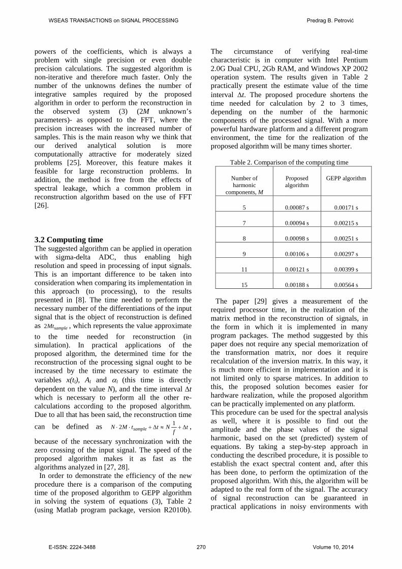
In order to demonstrate the efficiency of the new procedure there is a comparison of the computing time of the proposed algorithm to GEPP algorithm in solving the system of equations (3), Table 2 (using Matlab program package, version R2010b).

The circumstance of verifying real-time characteristic is in computer with Intel Pentium 2.0G Dual CPU, 2Gb RAM, and Windows XP 2002 operation system. The results given in Table 2 practically present the estimate value of the time interval ∆t. The proposed procedure shortens the time needed for calculation by 2 to 3 times, depending on the number of the harmonic components of the processed signal. With a more powerful hardware platform and a different program environment, the time for the realization of the proposed algorithm will be many times shorter.

Table 2. Comparison of the computing time

Number of harmonic

components, M

Proposed algorithm

GEPP algorithm

5 0.00087 s 0.00171 s

7 0.00094 s 0.00215 s

8 0.00098 s 0.00251 s

9 0.00106 s 0.00297 s

11 0.00121 s 0.00399 s

15 0.00188 s 0.00564 s

The paper [29] gives a measurement of the required processor time, in the realization of the matrix method in the reconstruction of signals, in the form in which it is implemented in many program packages. The method suggested by this paper does not require any special memorization of the transformation matrix, nor does it require recalculation of the inversion matrix. In this way, it is much more efficient in implementation and it is not limited only to sparse matrices. In addition to this, the proposed solution becomes easier for hardware realization, while the proposed algorithm can be practically implemented on any platform. This procedure can be used for the spectral analysis as well, where it is possible to find out the amplitude and the phase values of the signal harmonic, based on the set (predicted) system of equations. By taking a step-by-step approach in conducting the described procedure, it is possible to establish the exact spectral content and, after this has been done, to perform the optimization of the proposed algorithm. With this, the algorithm will be adapted to the real form of the signal. The accuracy of signal reconstruction can be guaranteed in practical applications in noisy environments with


E-ISSN: 2224-3488 270 Volume 10, 2014

the use of a powerful processor with adequate filtering. 4 Simulation Results The algorithm proposed in this paper is tested by means of the input data obtained through computer simulation. In order to investigate the statistical properties of the proposed estimator, noisy samples generated by computer simulation are used. Noisy samples are obtained by adding white noise samples to the samples of processing signal. For the estimation of deterministic parameters, a commonly used lower bound for the mean squared error (MSE) is the Cramer-Rao lower bound (CRLB), given by inverse of the Fisher information [30-32]. Fig. 3 and 4 respectively depict the MSE of the amplitudes and frequency after 105 simulations. Results clearly show that the proposed estimation scheme asymptotically reach the CRLB as in [32, 33].

Fig. 3. MSE of the frequency as a function of SNR.

Fig. 4. MSE of the three harmonic amplitudes as a function of SNR.

Additional testing of the proposed algorithm was carried out by simulation in the program package Matlab and SIMULINK. Standard sigma-delta ADC with the effective resolution of 24 bit, and sampling rate fS=1 kHz was used as the ADC. During the

simulation, the parameters of the input signal correspond to the values given in Table 3. The execution time of the proposed algorithm on hardware platform described earlier was 0.0167s. In the course of the simulation conducted in this way, the output PSD (Power Spectral Density) of the ideal, thermal noise affected and clock jitter affected was in the range of -100 to -170 dB for the signal-to-noise distortion ratio (SNDR) ranged between 55 dB and 76 dB.

Table 3. Comparison of simulation results by the proposed reconstruction algorithm, FFT and

continuous wavelet transformation (CWT) [37]

Harmonic number

Amplitude [VPP]

Phase [rad]

Proposed reconstruction algorithm

Amp.error [%]

Phase error [%]

1 1 π 0.0018 0.0019

2 0.81 π/3 0.0024 0.0022

3 0.62 0 0.0022 0.0021

4 0.58 π/6 0.0015 0.0016

5 0.41 π/4 0.0015 0.0021

6 0.33 π/12 0.0021 0.0019

7 0.16 0 0.0020 0.0022

Harmonic number

FFT (sampling rate = 25 kHz;data length =

25000; time period = 1 s)

CWT

Amp.error [%]

Phase error [%]

Amp.error [%]

Phase error [%]

1 0.296 0.322 0.023 0.034

2 0.035 0.038 0.032 0.028

3 0.875 0.843 0.049 0.026

4 0 0 0.144 0.012

5 0 0 0.013 0.154

6 0 0 0.012 0.017

7 0 0 0.223 0.186 A signal containing the first 7 harmonics was

used, with the fundamental frequency f = 50 Hz. The superposed noise and jitter will, in simulation performed in this way, cause a relative error in


E-ISSN: 2224-3488 271 Volume 10, 2014

detection on fundamental frequency of 0.001 %. It can be seen that the accuracy of the proposed algorithm is within the limits that are attained in processing a signal of this form, in [28, 32, 34-36], and better then the one presented in [37]. In the time domain, the relative error between the signal and its reconstruction was 0.0025 %. The errors in the amplitude and phase detection are mainly due to the error in measuring of the input signal samples and the error in determining the value of the derived equations. 4 Conclusion The algorithm proposed in this paper is a new complexity-reduced algorithm for estimation of the Fourier coefficient. The derived analytical expression opens a possibility to perform fast calculations of the basic parameters of signals (the phase and the amplitude), with a low numeric error. All the necessary hardware resources can be satisfied by a DSP of standard features and real sigma-delta ADC. The suggested concept can be used as a separate algorithm as well, for the spectral analysis of the processed signals. Based on the identified parameters of the ac signals, we can establish all the relevant values in the electric utilities (energy, power, RMS values). The measurement uncertainty is a function of the error in synchronization with fundamental frequency of processing signal (because of the no stationary nature of the jitter-related noise and white Gauss noise), and the error that occurs in determining the values of the differential samples of the processed signal. The simulation results show that the proposed algorithm can offer satisfactory precision in reconstruction of periodic signals in a real environment.

Acknowledgements The author wishes to thank to the Ministry of

Education and Science of the Republic of Serbia for its support of this work provided within the projects 42009 and OI-172057. References: [1]. J. G. Proakis and D. G. Manolakis, Digital

Signal Processing: Principles, Algorithms, Applications, 3rd ed. Englewood Cliffs, NJ: Prentice-Hall, 1996.

[2]. L.L.Lai, W.L. Chan, C.T.Tse, and A.T.P.SO, „Real-time frequency and harmonic evaluation using artifical neural networks“, IEEE Trans. on Power Delivery, 14, (1), 1999, pp.52-59

[3]. R. S. Prendergast, B. C. Levy, and P. J. Hurst, „Reconstruction of Band-Limited Periodic Nonuniformly Sampled Signals

Through Multirate Filter Banks“, IEEE Trans. Circ. Syst.-I,: 51, (8), 2004, pp.1612-1622

[4]. P. Marziliano, M. Vetterli, and T.

Blu, „Sampling and Exact Reconstruction of Bandlimited Signals With Additive Shot Noise“, IEEE Trans. Inform. Theory, 52, (5), 2006, pp.2230-2233

[5]. E. Margolis, Y. C. Eldar,

„Reconstruction of nonuniformly sampled periodic signals: algorithms and stability analysis“, Electronics, Circuits and Systems, 2004. ICECS 2004. Proceedings of the 2004 11th IEEE International Conference, 13-15 Dec. 2004, pp. 555-558

[6]. W. Sun and X. Zhou, „Reconstruction of Band-Limited Signals From Local Averages“, IEEE Trans. Inf. Theory, 48, (11), 2002, pp. 2955-2963

[7]. P. Petrovic, “New method and circuit for processing of band-limited periodic signals“Signal Image and Video Processing, Springer, 6, (1), 2012, pp. 109-123.

[8]. A.K. Muciek, „A Method for Precise RMS Measurements of Periodic Signals by Reconstruction Technique With Correction“, IEEE Trans. Instrum. Meas., 56, (2), 2007, pp.513-516

[9]. A.V.D.Bos, „Estimation of Fourier Coefficients“, IEEE Trans. Instrum. Meas., 38, (5), 1989, pp.1005-1007

[10]. A.V.D.Bos, „Estimation of complex Fourier Coefficients“, IEE Proc.-Control Theory Appl., 142, (3), 1995, pp.253-256

[11]. R. Pintelon, and J. Schoukens, „An Improved Sine-Wave Fitting Procedure for Characterizing Data Acquisition Channels“, IEEE Trans. Instrum. Meas., 45, (2), 1996, pp.588-593

[12]. Y. Xiao, Y. Tadokaro, and K. Shida, „Adaptive Algorithm Based on Least Mean p-Power Error Criteterion for Fourier Analysis in Additive Noise“, IEEE Trans. Signal Proc., 47, (4), 1999, pp.1172-1181

[13]. P. Arpaia, A. Cruz Serra, P. Daponte, and C.L. Monteiro, „A critical note to IEEE 1057-94


E-ISSN: 2224-3488 272 Volume 10, 2014

standard on hysteretic ADC dynamic testing“, IEEE Trans. Instrum. Meas., 50, (4), 2001, pp. 941-948.

[14]. G. Seber, Linear Regression Analysis, New York; Wiley, 1977.

[15]. S.J.Reeves and L. P. Heck, „Selection of Observations in Signal Reconstruction“, IEEE Trans. Signal Proc., 43, (3), 1995, pp.788-791

[16]. Y. S. Poberezhskiy and G. Y. Poberezhskiy, „Sampling and Signal Reconstruction Circuits Performing Internal Antialiasing Filtering and Their Influence on the Design of Digital Receivers and Transmitters“, IEEE Trans. Circ. Sys.-I, 51, (1), 2004, pp. 118-129

[17]. Y. Xiao, R. K. Ward, L. Ma, and A. Ikuta, “A New LMS-Based Fourier Analyzer in the Presence of Frequency Mismatch and Applications”, IEEE Trans. Circ. Syst.-I, 52, (1), 2005, pp.230-245

[18]. Y. Xiao, R.K. Ward, and L. Xu, “A new LMS-based Fourier analyzer in the presence of frequency mismatch”, ISCAS’03, Proceedings of the 2003 International Symposium on Circuits and Systems, vol. 4, 2003, pp.369-372.

[19]. H. C. So, K. W. Chan, Y. T. Chan,

and K. C. Ho, „Linear Prediction

Approach for Efficient Frequency

Estimation of Multiple Real Sinusoids:

Algorithms and Analyses“, IEEE Trans. Signal Proc., 53, (7), 2005, pp.2290-2305

[20]. B. Wu and M. Bodson, "Frequency estimation using multiple source and multiple harmonic components", American Control Conference, 2002. Proceedings of the 2002, vol.1, 8-10 May 2002, pp. 21-22

[21]. L. Tan, and L. Wang, „Oversampling Technique for Obtaining Higher Order Derivative of Low-Frequency Signals“, IEEE Trans. Instrum. and Meas.,60, (11), 2011, pp. 3677-3684.

[22]. P. Petrovic, „New Digital Multimeter for Accurate Measurement of Synchronously Sampled AC Signals“, IEEE Trans. Instrum. Meas., 53, (3), 2004, pp.716-725

[23]. T. Daboczi, “Uncertainty of Signal Reconstruction in the Case of Jitter and Noisy Measurements”, IEEE Trans.on Instrum.Meas., 47, (5), 1998, pp.1062-1066

[24]. G. Wang, W. Han, “Minimum Error Bound of Signal Reconstruction”, IEEE Signal Proc. Lett., 6, (12), 1999, pp. 309-311

[25]. N. J. Nigham, Accuracy and Stability of Numerical Algorithms, 2nd ed, SIAM, 2002.

[26]. H. G. Feichtinger, „Reconstruction of band-limited signals from irregular samples, a short summary“, 2nd International Workshop on Digital Image Processing and Computer Graphics with Applications, 1991, pp. 52-60.

[27]. T. Cooklev, „An Efficient Architecture for Orthogonal Wavlet Transforms“, IEEE Signal Proc. Lett., 13, (2), 2006, pp. 77-79

[28]. J. Schoukens, Y. Rolain, G. Simon, and R. Pintelon, „Fully Automated Spectral Analysis of Periodic Signals, IEEE Trans. Instrum. Meas., 52, (4), 2003, pp.1021-1024

[29]. S. J. Reeves, „An Efficient Implementation of the Backward Greedy Algorithm for Sparse Signal Reconstruction“, IEEE Signal Proc. Lett., 6, (10), 1999, pp. 266-268

[30]. S. M. Kay, Modern Spectral estimation: Theory and Applications, Englewood Cliffs, NJ: Prentice-Hall, 1988.

[31]. P. Stoica, H. Li, and J. Lim, “Amplitude estimation of sinusoidal signals: Survey, new results, and an application”, IEEE Trans. Signal Process., 48, (2), 2000, pp. 338-352.

[32]. D. Belega, D. Dallet, and D. Slepicka, “Accurate Amplitude Estimation of Harmonic Components of Incoherently Sampled Signals in the Frequency Domain”, IEEE Trans. on Instr. and Meas., 59, (5), 2010, pp. 1158-1166.

[33]. Y. Pantazis, O. Roces, and Y. Stylianou, “Iterative Estimation of sinusoidal Signal Parameters”, IEEE Signal Process. Lett., 17, (5), 2010, pp.461-464.

[34]. R. M. Hidalgo, J. G. Fernandez, R.R. Rivera, and H.A. Larrondo, “A Simple Adjustable Window Algorithm to Improve FFT Measurements”, IEEE Trans. Instrum. Meas., 51, (1), 1996, pp. 31-36.

[35]. D. Agrež, “Weighted Multi-Point Interpolated DFT to Improve Amplitude Estimation of Multi-Frequency Signal”, IEEE Trans. on Instr. and Meas., 51, 2002, pp. 287-292.

[36]. D. Agrež, “Improving phase estimation with leakage minimization” IEEE Trans. on Instr. and Meas., 54, (4), 2005, pp. 1347-1353.

[37]. N.C.F. Tse, and L. L Lai, “Wavelet-Based Algorithm for Signal Analysis”, EURASIP Journal on Advances in Signal Processing, 2007, Article ID 38916, 10 pages.

Appendix

For MqMp ≤≤∧≤≤ 121 :


E-ISSN: 2224-3488 273 Volume 10, 2014

( ) ( )

( ) ( ) ( ) ( )

( ) ( ) ( ) ( )

( ) ( )

( ) ( ) ( )

( )( ) ( ) ( )

( ) ( )

( )( )

( )( ) ( ) ( ) ( )

( ) ( ) ( ) ( )

( )( )

( ) ( ) ( )( ) ijejxqMpMM

qMpMM

iMppMiM

M

MM

p

iMiMiMiqMiqM

p

iMiqMiqMiMiM

iMppMiM

M

MM

p

iMiiiqiqiM

p

iMiqiqiiiMiM

M

MM

p

iMiqiqiiMiM

p

iMiiMiqiqi

M

iM

p

iMiqiqiqiqiiMiqiqiM

iM

p

iMiMiiiMiMiqiqiqiqiiM

iM

p

qp

ee

eeeee

eeeeeee

eeeeee

eeeeeee

eeeeee

eeeeeee

eeeeeeeeeee

eeeeeeeeeeeee

MMqq

ϕϕϕϕϕ

π

ϕϕϕϕϕ

ϕϕϕϕϕ

ϕϕϕϕπ

ϕϕϕϕϕϕ

ϕϕϕϕϕϕπ

ϕϕϕϕϕϕ

ϕϕϕϕϕϕπ


π


π

ϕϕϕϕϕϕ

=

+−++

+++

++++−++−−+

+−+−−−

++−++−

++++−++−−+

−−−+−−

+−−−

−+

+−−−

−+−−−−−

+−−−+−−−−

−

−−−+−+−−−−

−

−

∆−∆−

=

=

−

−−=

=

−

−−=

=

−+

+=

=−=

=−−++++=

=+−=

1,1,12

,1,12

2...11...122

1

1211111111

1211111111

2...11...122

1

11111111

11111111

22

1

11111111

111111112

111111111111112

111111111111111112

2

111111

21

.........1

.........1

21

.........

.........

21

.........1

.........

2

............2

.........2

sin...sincos...1cos1cos...cosF

(21)

It follows that:

( )( )

( ) ( ) ( )( ) MqMpforee ijejxqMpMM

qMpMM

iMppMiM

M

MM

qp ≤≤∧≤≤∆−∆

−=

=

+−++

+++

++++−++−−+

1212

1 1,1,12

,1,12

2...11...122

1

ϕϕϕϕϕ

π

F (22)

where ( )srMM

,1,12 ++∆ is the determinant obtained from 1,12 ++∆ MM after the r row and s column have been

eliminated.

( ) ( ) ( )∑∏ ∏

−=∆

⇒=∆

+=

−

=++

+−

+−

++

MMM

M

kj

M

kkjMM

MM

MM

MMM

MMM

MM

xxxxxxxx

xxxx

xxxx

221221

2

1

12

11,12

22

12

122

21

11

111

1,12

...1...

......1.....................

......1

(23)

When we determinate ( )srMM

,1,12 ++∆ , we must eliminate r row and s column from 1,12 ++∆ MM , and if 1,12 ++∆ MM is

developed by r row, what we obtain is that ( ) ( )srMM

srsrD ,

1,12, 1 +++ ∆−= is the coefficient in ( )Msxs

r ≤≤− 11 , i.e. the

coefficient beside srx if MsM 21 ≤≤+ .

( ) ( ) ( )( ) ( ) ( ) ( ) ( )∑∏ ∏

−−−−−−=∆

≠≤≤ ≤≤

+−++MM

M

rjkMj

jkMk

kjMrrrrrrr

MM xxxxxxxxxxxxxxxx

221221

,21 21

21111,12 ...1.........1

(24)

Here is:


E-ISSN: 2224-3488 274 Volume 10, 2014

( ) ( ) ( ) ( ) ( )

( ) ( ) ( )( ) ( )

( ) ( )

Msfor

xxxxxxxx

xxxxxxxx

xxxxxx

xxxxxxxxxxxxxx

xxxxxx

MMrrsMMrr

MMrrsMMrr

Mrr

rjkMj

jkMk

kjsr

MM

MMrrrMMrrrMrr

MMM

≤≤

⋅−

−⋅

−=∆

⇒

+⋅⋅=

∑ ∑

∑ ∑∏ ∏

∑ ∑∑

+−+−+−

−+−−+−

+−

≠≤≤ ≤≤

++

−+−+−+−

1

......1......

......1......

......

......11

......1......

...1...

2111122111

1211122111

2111

,21 21

,1,12

1211121112111

221221

(25)

If we introduce the following symbols:

( )

( ) ijj

ijj

extMrr

t

extMrrt

xxxxV

xxxxV

ϕ

ϕ

=+−

=+−

∑

∑

=

=

2111

2111

......1

......

(26)

It follows that:

( ) ( ) ( ) ( )( )

( )MppMM

exMqMMqMMpp

pjkMj

jkMk

kji

tqMpMM

xxxxVVMq

forwhileMqforVVVVxxxxxxex itt

t

2111122

112111

,21 21

1,1,12

......;0

,11......

+−−

=+−−++−

≠≤≤ ≤≤

+−++

==⇒=

−≤≤−

−==∆ ∏ ∏ ϕϕ

(27)

We can write that:

( ) ( ) ( ) ( )( )

1;011

,21......

010

112111

,21 21

,1,12

==⇒==⇒−=

−≤≤−

−−==∆

−

=−−−−+−

≠≤≤ ≤≤

+++ ∏ ∏

VVMqforandVMq

forwhileMqforVVVVxxxxxxex itetxMqMMqMMpp

pjkMj

jkMk

kjit

tqMpMM ϕ

ϕ

(28)

From this, it follows that:

( )( )

( ) ( ) ( ) ( )( ) itetx

MqMMqM

MqMMqM

Mpp

pjkMj

jkMk

kjiMppMiM

M

MM

qp VVVV

VVVVxxxxxxee ϕ

ϕϕϕϕπ

=−−−−

−−++

+−

≠≤≤ ≤≤

++++−++−−+

−+

+−

−

−= ∏ ∏

11

11

2111

,21 21

2...11...122

1

......2

1

F (29)

( ) ( )( )

( )∏∏∏

∏ ∏≠≤≤

+=

−

=

=

≠≤≤ ≤≤ −

−−=

−

pkMk

ikip

M

kj

M

k

ikij

pitetx

pjkMj

jkMk

kj ee

eexx

21

2

1

12

1

,21 21

1ϕϕ

ϕϕ

ϕ

(30)

We can write that:

( ) ( ) ( ) ( )

( ) ( )

( ) ( ) ( ) ( )( )

( ) ( )( ) ( ) ( ){ }1111

21

2

1

12

1142221

21

2

1

12

12...11...11132221

,21 21

21

2...11...121

212

212

12

21

2

1

12

1

2...1212

2122

1

12

1

2sin

2sin

211

2sin

2sin

21

2sin2

2sin21

−−−−−−++

≠≤≤

+=

−

=+−−

≠≤≤

+=

−

=++++−+−+−−−

=

≠≤≤ ≤≤

≠≤≤

++++−+−−

−

≠≤≤

+=

−

=

++−

−−

+=

−

=

−+−⋅−

−

⋅−−=

⇒−

−

−=

−

⇒−

=−

−−=−

∏

∏∏

∏

∏∏∏ ∏

∏∏

∏∏∏∏

MqMMqMMqMMqM

pkMk

kp

M

kj

M

k

kj

MMMMpq

p

pkMk

kp

M

kj

M

k

kj

iMppMMMiMpitetx

pjkMj

jkMk

kj

pkMk

kpiMppipMiM

M

pkMk

ikip

M

kj

M

k

kjiMMiMMMM

M

kj

M

k

ikij

VVVVVVVVi

eexx

eeeee

eeee

ϕϕ

ϕϕ

ϕϕ

ϕϕ

ϕϕ

ϕϕ

ϕϕϕϕπ

ϕ

ϕϕϕϕϕπϕϕ

ϕϕπϕϕ

F

(31)


E-ISSN: 2224-3488 275 Volume 10, 2014

It follows that:

( ) ( ) ( ){ }( ) ( )∑∏

++−++

⋅−+−−

⋅−

= −−−−−−++

≠≤≤

−

MMMM

MqMMqMMqMMqM

pkMk

kpM

q

M

qp VVVVVVVVi

2121

1111

21

122 ......

21cos

1

2sin2

1

ϕϕϕϕϕϕX

X (32)

If we introduce the following symbols:

( )

( ) ( ) ( )

( ) ( ) ( )

( ) ( )

( ) ( ) ( ) ( )( ) ( )qMqMMqMqMM

qMqMqMqMMqMqMqMqMMMqMMqMMqMMqM

MMMMMMMqMqMqMqM

qMqMqMqM

qMqMqM

MqMMqMMqMMqMMqMMqMMqMMqM

tMppMppttp

t

tMppMppttp

t

ttt

iMpp

t

AAiBBBiACCCCiBCCCCAVVVVVVVV

BBAAiBACCCCC

BBAAiBAC

CCCCCCCCVVVVVVVV

BB

AA

iBAVeC

−−−−−−

−−−−−−−−−−−−−−−−−−++

−−−−−−−+−−+

−−+−−+

+++

−−−−−−++−−−−−−++

+−+−

+−+−

++++−++

++−=

=++++−+−=−+−

⇒−==+===

⇒−==

−=

−+−=−+−

⇒

+++++−+++++==

+++++−+++++==

+==

∑

∑

11

11111111

1111111

11

11111111

21112111

21112111

2...11...121

22

;;;;

;

............21sin

............21cos

ϕϕϕϕϕϕϕϕ

ϕϕϕϕϕϕϕϕ

ϕϕϕϕ

(33)

It follows that:

( ) ( ) ( ) ( )( ) ( ) ( ) ( )( )( ) ( )

21;......

21cos

2sin2

1

212121

11

22

1

2

−≤≤

++−++

−++−

⋅−

=

∑∏≠≤≤

−−−−−−

−

+

MqforAABBBA

MMMM

pkMk

kp

pqM

pqM

pM

pqM

pqM

pM

M

q

M

qp

ϕϕϕϕϕϕX

X (34)

In addition, for:

( )

( ) ( )( )beforeassametheareBandABACVMq

BA

eCVMq

MppMpp

iMpp

001111

2111021110

2...11...121

00

0;00

......21sin;......

21cos

;11

===⇒=⇒=

+++++=+++++=

==⇒−=

−−−−

+−+−

++++−++

ϕϕϕϕϕϕϕϕ

ϕϕϕϕ

(35)

Now, we can determine co-factors qpF for MqMMp 21;21 ≤≤+≤≤ , and qM

p+F for Mq ≤≤1 . As above, we

obtain that:

( )( )

( ) ( ) ( ) ( )( ) ijejxqMpMM

qMpMM

iMppMiM

M

MM

qp ee ϕ

ϕϕϕϕπ

=

+−++

+++

++++−++−−−+

∆−∆−

= 1,1,12

,1,12

2...11...1212

1

21F (36)

From this, it follows that:

( ) ( ) ( ) ( )( ) ( ) ( ) ( )( )( ) ( )∑∏

++−++⋅

−++−

⋅−

=

≠≤≤

−−−−−−

−

++

MMMM

pkMk

kp

pqM

pqM

pM

pqM

pqM

pM

M

q

M

qMp BBBAAA

212121

1122

1

2 ......21cos

2sin2

1

ϕϕϕϕϕϕX

X (37)


E-ISSN: 2224-3488 276 Volume 10, 2014

algorithm for signal parameters estimation based … · algorithm for signal parameters estimation...

Documents