Terascale Data Organization for Discovering MultivariateClimatic Trends

Wesley Kendall, Markus Glatter, andJian Huang

Department of Electrical Engineering andComputer Science

The University of Tennessee, KnoxvilleKnoxville, TN 37996

{kendall, glatter, huangj}@eecs.utk.edu

Tom Peterka, Robert Latham, andRobert Ross

Mathematics and Computer Science DivisionArgonne National Laboratory

Argonne, IL 60439{tpeterka, robl, rross}@mcs.anl.gov

ABSTRACTCurrent visualization tools lack the ability to perform full-range spatial and temporal analysis on terascale scientificdatasets. Two key reasons exist for this shortcoming: I/Oand postprocessing on these datasets are being performedin suboptimal manners, and the subsequent data extractionand analysis routines have not been studied in depth at largescales. We resolved these issues through advanced I/O tech-niques and improvements to current query-driven visualiza-tion methods. We show the efficiency of our approach byanalyzing over a terabyte of multivariate satellite data andaddressing two key issues in climate science: time-lag anal-ysis and drought assessment. Our methods allowed us toreduce the end-to-end execution times on these problems toone minute on a Cray XT4 machine.

KeywordsQuery-Driven Visualization, Parallel I/O, Temporal DataAnalysis, MODIS

1. INTRODUCTIONTo understand the underlying structures and relationshipsof variables in datasets through space and time, it is oftennecessary to analyze and visualize the full spatial and tem-poral extent of the dataset. The need for scalable methodsto perform such full-range analysis tasks is growing as sci-entific simulations produce datasets ranging to the terascaleand beyond. This need is particularly acute as visualizationapplications, especially those that handle large-scale time-varying data, are increasingly being dominated by I/O over-heads to a degree that impedes their practical use.

As an example of the challenge that I/O presents in visu-alization, [1] has shown that rendering a single timestep ofa 20483 volume can be optimized to take only a few sec-

Permission to make digital or hard copies of all or part of this work forpersonal or classroom use is granted without fee provided that copiesare not made or distributed for profit or commercial advantage, and thatcopies bear this notice and the full citation on the first page. Copyrightsfor components of this work owned by others than ACM must be honored.Abstracting with credit is permitted. To copy otherwise, to republish, topost on servers or to redistribute to lists, requires prior specific permissionand/or a fee.

SC09 November 14-20, 2009, Portland, Oregon, USA(c) 2009 ACM 978-1-60558-744-8/09/11. . . $10.00

onds on an IBM Blue Gene/P, however, reading that volumefrom disk takes at least a minute. Efficient I/O solutions areneeded if one wishes to perform more complex visualizationand analysis tasks that involve many timesteps to be loadedat once. In order for visualization to make a greater impacton terascale computational science, I/O cannot be treatedin isolation.

In this work, we developed a system that closely integratedtechniques in parallel I/O with concepts from parallel query-driven visualization. Our contributions include: first, to al-leviate I/O bottlenecks in full-range analysis through ad-vanced methods of performing I/O on common scientificdata storage formats; second, to scale parallel extractionof salient spatial and temporal regions in scientific datasetsby improving current parallel data querying techniques; andthird, to assess multivariate relationships in terascale obser-vational data by using our techniques to alleviate computingand I/O overheads.

The scalability of our system enabled us to explore over aterabyte of multivariate satellite data from NASA’s Mod-erate Resolution Imaging Spectroradiometer (MODIS) [2]project. The amount of data and the desired combinatorialway of exploring for conceptual events, such as prolongedperiods of drought and event relationships, required usingcomputing resources at large scale.

With scalability up to 16K cores, our full-range studies on≈1.1 TB of MODIS were optimized to take around oneminute. This time includes all stages of the pipeline, fromthe initial I/O operations to the resulting visualization. Theability to perform these complex analysis tasks at large scaleson datasets directly from simulations provides a flexibilitythat is not offered by current visualization tools. The follow-ing discusses our work in reducing the end-to-end latency ofthese complex analyses.

Figure 1: An overview of our system.

2. OVERVIEW AND RELATED WORKOur work primarily spans the fields of parallel I/O, featuretracking, and parallel query-driven visualization. Little re-search exists that systematically combines these areas, andeach area is crucial for our driving application. Before dis-cussing the relevant related work, we present a synopsis ofthe driving application and our system, along with a de-scription of the Cray XT4 machine we used.

2.1 The Driving ApplicationOur driving application is to study observational data inNASA’s MODIS database to discover multivariate climatictrends. The dataset used in our study consists of a 500 meterresolution sampling of North and South America, creatinga 31,200 by 21,600 grid. The dataset is continuously up-dated, and we used 417 timesteps of 8 day intervals fromFebruary 2000 to February 2009. MODIS data is storedin various wavelength bands which may be used to computeother variables. By computing two variables that are relatedto our studies in Section 5 and storing them as short inte-gers, the entire dataset totals to ≈1.1 TB. With a datasetof this magnitude, we have two primary goals: to providevisualization and analysis methods for cases when many ofthe timesteps of the dataset need to be loaded, and to de-liver usability and near-interactive functionality specificallyfor application scientists.

The visualization aspect of this task is very demanding forseveral reasons. First, extracting isocontours with an inher-ent temporal component is rather new in the field. Drought,for instance, is not a single timestep event and requires “ab-normally low rainfall” to have lasted for a period of time. Al-though tracking contours over time has already been solved[3], visualization typically still treats contour extraction stat-ically in the spatial domain [4]. We instead seek for spatiallocations in a contour that fit two criteria: thresholds forscalar variables, and the number of continuous timesteps

that meet the first criteria. Advanced data structures arenecessary to allow for such high dimensional searches. Un-fortunately, the most likely methods and data structures,particularly those used in query-driven visualization, incurpreprocessing overheads on the order of several hours fordatasets of 100 GB [5, 6, 7].

Second, current data analysis tools are not efficiently inte-grated with system level tools such as parallel I/O. Thiscauses a severe bottleneck in efforts to shorten the end-to-end latency as outlined by the vision of in situ analysis andvisualization [8]. In addition, few current data analysis toolshave the scalability to leverage modern systems, such as theCray XT4 and the IBM Blue Gene/P. Not being able to fullyleverage systems of that caliber, especially the next genera-tion storage and parallel I/O systems, imposes yet anotherbottleneck in obtaining the full potential of data analysistools in production scientific use.

Third, typical user work flow includes an often neglected butvery expensive component. That is, to get the datasets froman application-native format into a format that is the mostamenable to the parallel data analysis or visualization. Tominimize the end-to-end latency, this step must be studiedin depth. In this work, we specifically focused on one of themost common cases of our collaborators, where individualtimesteps are initially stored in separate netCDF files.

Figure 1 illustrates the overall architecture of our data anal-ysis system. When data is produced, it is stored in anapplication-native format and striped across the parallel filesystem for higher access bandwidth. Our system reads anddistributes data in parallel to prepare it into a queriableform with maximal runtime load balance. The relevant datais then queried and spatial or temporal analysis may occurby sorting the data in the proper ordering.

The system provides a means for analysis to take placeon datasets immediately after being written to disk, andit also reduces computing overheads by using query-drivenconcepts to access only the data deemed relevant. By usingthese concepts, problems of full-range analysis and visualiza-tion on terascale datasets can be solved in feasible amountsof time. In the following, we further discuss our targetedinfrastructure and the previous works that have influencedour design decisions.

2.2 Targeted InfrastructureIn our study, we used the Jaguar Cray XT4 machine locatedat Oak Ridge National Laboratory as a testing ground forour methods. Jaguar consists of 7,832 quad-core 2.1 GHzAMD Opteron processors with 8 GB of memory. The sys-tem totals to 31,328 cores with 62 TB of main memory.The parallel file system on Jaguar is the Lustre file sys-tem [9]. Lustre is an object-based parallel file system, con-sisting of Object Storage Servers (OSSs) that handle I/Orequests from the clients to the actual storage. Each OSSserves one or more Object Storage Targets (OSTs), whichare the physical disks. Lustre uses one Metadata Server(MDS) that holds the file information for the entire system.Jaguar’s Lustre file system contains 72 OSSs that serve 144OSTs.

2.3 In Situ Processing and VisualizationMa et al. [8] described the various bottlenecks present inpopular methods of large data processing and visualization.The authors emphasized the importance of being able tocouple visualization and analysis into the simulation pipeline.This allows for reduction of data and valuable analysis dur-ing the simulation that can further accelerate the scientificdiscovery process.

The authors further discussed various postprocessing stepsthat are common in the visualization and analysis pipeline.With in situ visualization, many of these steps can be re-duced or even taken out. Although we do not couple ourcode directly with simulation code, we provide a means to in-teract with data written directly from the simulation, alongwith conducting postprocessing on the fly.

2.4 Parallel I/OSignificant algorithmic advances have improved the usabil-ity and portability of parallel I/O across high-performancesystems, and user-friendly interfaces have been developed toaid in achieving higher I/O bandwidths. I/O interfaces builton top of the MPI-2 [10] standard, such as ROMIO [11], haveshown various optimizations that can be applied to the I/Ophase for various parallel data access patterns. CollectiveI/O and data sieving are such examples [11]. We used opti-mizations such as collective I/O as a means to achieve betterbandwidth rates in our I/O phase.

I/O has recently been gaining more attention in visualiza-tion research. Ma et al. [12] first showed how overlappingI/O with rendering could significantly reduce interframe de-lay in the parallel rendering of large-scale earthquake simu-lations. Yu et al. [13] extended this by presenting I/O solu-tions for a parallel visualization pipeline. Yu et al. [14] alsopresented two parallel I/O methods for the visualization of

time-varying volume data in a high-performance computingenvironment.

Peterka et al. [1] have recently performed extensive work onlarge-scale parallel volume rendering of astrophysics data onthe IBM Blue Gene/P. Their method of visualization focusedon efficiently using parallel I/O to increase frame rates. Byusing a system like the Blue Gene/P, the authors showedthat a simulation-caliber resource is a valuable alternativeto a graphics cluster for visualization, especially when I/Ois the bottleneck.

Although our primary systems need is to efficiently read datafrom storage and organize it in memory, we are aware of sys-tematic efforts underway to address challenges of outputtingdata by scientific simulations at the petascale. One effort inthat regard is the Adaptive I/O System (ADIOS) [15], whichprovides input and output performance gains and a flexibil-ity of runtime choices of different I/O methods and dataformats. Systems like ADIOS can treat visualization as justanother I/O method, enabling in situ visualization.

2.5 Feature Extraction and TrackingOne of the most widespread uses of feature detection in visu-alization is to extract isocontours from scalar fields. Isocon-tour extraction can be explicit or implicit. Volume renderingmethods [21] implicitly extract isocontours by using transferfunctions to assign non-zero opacity only to a few selectedcontinuous narrow ranges of scalar values. The marchingcube algorithm [4] explicitly constructs the geometry thatcorresponds to one single scalar value or a continuous rangeof scalar values.

Silver et al. first tracked explicitly extracted features overtime [3]. By finding spatial overlaps between features fromneighboring timesteps, their methods discovered the evolu-tionary history of contours. Tzeng and Ma [22] were thefirst to demonstrate that features evolve not only spatiallybut also in value space over time. In other words, the valuesthat define the contours of a feature do not remain con-stant across all timesteps. Thus, features cannot be reli-ably tracked without considering the variations in the val-ues of the isocontours. We know of no previous research thathas considered directly extracting contours with an inherenttemporal element, such as the drought problem discussed inSection 5.

2.6 Query-Driven VisualizationQuery-driven visualization [5, 16, 17, 6, 7] has recently be-come a popular research topic. Query-driven methods arerelated to feature extraction in several of ways. First, query-driven methods rely on translating a user interest into a com-pound Boolean range query. In doing so, it offers a naturalextension of feature extraction capabilities in multivariatedata. Second, regardless of the underlying methods, such asa distributed M-ary search tree [5], bitmap indexing [7] orbin-hashing [6], query-driven visualization has been shownto accelerate contour extraction in large datasets. The meth-ods for query-driven visualization can be split into two cat-egories: tree-based and index-based methods.

In indexed-based methods [18, 7, 19], bitmap indexing isused to accelerate the search phase. To build the index,

each record r with v distinct attribute values generates vbitmaps with r values each. This allows for bitwise logicaloperations to be performed on range queries, making mul-tivariate range queries simple linear combinations of single-valued queries [7]. In tree-based methods, data is sorted andindexed with tree structures such as B-trees or M-ary searchtree structures [5].

It has been shown that tree-based methods suffer from the“Curse of Dimensionality”, where adding more dimensionsresults in an exponential growth in storage and process-ing requirements [7]. Although this is true for a naive treemethod, Glatter et al. [5] showed how an M-ary search treestructure could be used to reduce the storage overhead toless than 1% of the dataset size and also showed that theoverhead is not dependent on the dataset size. This factoris attractive to our method of querying since we load thedata in main memory. It was also shown in [5] that queriescould be load balanced by distributing data on the granu-larity of single voxels. Although parallel methods of index-based query-driven visualization have been established [18,19], these do not focus on the issue of load balanced data ex-traction. Since load balancing is crucial to the performanceof our system, we used [5] as the background for our parallelquerying model.

2.7 Parallel SortingWe used parallel sorting for applying two of our load bal-ancing schemes discussed in Section 4, and for performingparallel temporal analysis discussed in Section 5. Becauseof the results in the seminal work by Blelloch et al. [20], wechose to use the parallel sample sort algorithm.

The parallel sample sort algorithm randomly samples thedataset choosing samples in such a way to linearly split theentire dataset. The processes then bin their data based onthe splitter samples and sort their bins, creating a glob-ally sorted list. Parallel sorting is an inherently network-intensive process, and this algorithm sums up all of its net-work communication in one MPI Alltoall call to bin thedataset. To locally sort the bins, we used the quick sortalgorithm.

3. THE I/O COMPONENTVisualization applications are often dominated by I/O timewhen working with terascale datasets, and this can be exac-erbated with simplistic methods such as pushing the entireI/O request through one node [23]. We used an advancedmethod for performing I/O on application-native formats toreduce I/O costs and allow for analysis with no postprocess-ing step.

3.1 Design ConsiderationsIt is common for our collaborators to use the netCDF [24]format to store their data, so we used the Parallel netCDFlibrary [25] as a layer for our disk access. This library isbuilt on top of MPI-2 [10], allowing it to execute on a widevariety of high-performance architectures independent of theparallel file system that is installed.

Another common storage method for our collaborators is tostore a separate file for each timestep or variable. Thus,

it is necessary to have an algorithm that performs I/O onmultiple files in an efficient manner. The research that mostclosely resembles our work is by Memik et al. in [26], wherethey examine reducing I/O and data transfer times in col-lective methods to multiple files. They showed this problemwas NP-complete when the files were arbitrary sizes and pro-vided various solutions to the problem. In our system, theassignment of data to processes is irrelevant, and we onlyrequire that all the data be loaded in memory after the I/Ostep. Because of this, the step of minimization of transfer-ring data to the correct process shown in [26] was not needed,and we were able to create a more general algorithm.

It was shown in [26] that a greedy heuristic could be usedwhen assigning processes to files. We used a similar ap-proach and applied a greedy heuristic that maximizes theamount of complete files that can be read at one time. Weused this heuristic because it allows us to perform large col-lective reads on the files and efficiently use collective I/Ostrategies implemented in ROMIO [11]. Collective I/O isuseful primarily for three reasons. First, it was shown in [27]that parallel opening of shared files is much more effectiveon large amounts of OSTs. Second, collective I/O can re-sult in larger reads that result in higher bandwidths. Third,we can tune the size of the collective I/O buffer for betterbandwidths. We used a buffer size of 32 MB because of theresults obtained in [27].

3.2 Greedy I/O on Multiple FilesOur approach for performing I/O on multiple files is notlimited by the number of processes or the number of files.The routine proceeds in the following steps:

1. A configuration file is read with information about thedataset. This information includes the directory wheredata is stored, the variables of interest, restrictions orsubsampling rates on the dimensions of the variables,and the ranges of variables that are unimportant.

2. Each file is assigned round robin to the N processes.The files are opened by the respective processes, andthe metadata about the all the variables is gathered.The total size of the dataset D is computed, and eachprocess must read in approximately Q amount of datawhere Q = D

N. Each process P contains DP amount

of data that has been read in, with DP starting at 0.

3. The first process P that has DP < Q reserves thelargest chunk possible of the first file F that has notyet been fully read in. If sizeof(F ) ≤ Q−DP , P willbe able to reserve all of the data available to read in F .If sizeof(F ) > Q−DP , P will reserve Q−DP amountof data from F . This will continue on the remainingprocesses where DP < Q until all of F is reserved oruntil no more processes are available.

4. Once a group of processes has been assigned to a file,an MPI communicator is created for the group and col-lective parallel I/O is performed on the variables. Foreach process P that performed I/O, DP is incrementedby the amount of data read in.

5. If DP < Q, process P repeats steps 3 and 4 with theremaining files in subsequent stages. This continuesuntil all processes have read in Q amount of data.

Figure 2: Example of the greedy I/O algorithm withfour processes and three files.

The greedy approach is best shown by a simple example inFigure 2. This example conducts the algorithm on three fileswhile using four processes. In stage S0, P0 and P2 are ableto read in their respective Q amount of data. P1 and P3

are not able to do this, so they continue to the next stageS1. In this stage, they read in F2 and finish reading in theirrespective Q amount of data.

The main limitation of this algorithm is the amount of datathat can be loaded in the aggregate memory of the nodes.Two strategies are provided to address this issue. First,users are able to specify ranges of variables that are irrel-evant to their analysis in the dataset configuration. Sincethe algorithm executes in stages, these values are filteredbetween stages, thus using memory more efficiently. Sec-ond, subsampling rates or restrictions may be specified inthe dataset configuration and applied to the dimensions, en-abling a reduced version of the dataset to be read in.

3.3 Results and ComparisonsWe tested the bandwidth rates for this algorithm on varyingscales with the MODIS dataset. If the aggregate memoryof the nodes was insufficient, data was discarded after beingread in for bandwidth testing purposes. It is difficult to com-pare the bandwidth rates of our algorithm with benchmarkresults on the Jaguar machine because netCDF benchmarksdo not exist for this machine. Therefore, we compare ourresults with the IOR benchmark [28] results obtained in [27]as a comparison for how our algorithm performs at largescales.

The IOR benchmark provides the ability to test aggregateI/O rates with MPI collective I/O calls on various file ac-cess modes and access patterns. In [27], the authors usedthe IOR benchmark on Jaguar to show how the bandwidthscales when using varying amounts of OSTs to read in data.We use the bandwidth results obtained from using 144 OSTsin [27] as a comparison since we also used 144 OSTs. Twobenchmarks from [27] using 1K cores showed bandwidthrates of ≈42 GB/s when reading in one shared file and ≈36

0

5,000

10,000

15,000

20,000

25,000

30,000

16 32 64 128 256 512 1K 2K 4K 8K 16K

MB

/s

Cores

I/O Bandwidth Results

Figure 3: I/O bandwidth results for the greedy al-gorithm on the MODIS dataset.

GB/s when reading in one file per process. Other bench-marks were conducted that used greater than 1K cores, butthe amount of OSTs used was not explicitly stated and thebandwidth rates were less than those of the IOR benchmark.

Bandwidth results of our algorithm are shown in Figure 3.When timing the results, the files were first opened and thentiming was started after an MPI Barrier. After all the I/Owas complete, another MPI Barrier was called and timingstopped. We achieved up to ≈28 GB/s on 4K cores, roughly75% of the 42 GB/s benchmark comparison. The bandwidthbottomed out around 2K cores, and performance degrada-tion was seen when scaling to 8K and 16K cores. This sametrend was observed in [27] on a separate benchmark. Wehypothesize that the MDS was being overwhelmed with re-quests when going to this scale, but further testing is re-quired to confirm this.

When scaling to 4K cores, we were able to minimize the I/Otime on the entire 1.1 TB MODIS dataset to ≈37 seconds.The results show that using collective I/O combined with agreedy approach to saturate the underlying I/O system withrequests can achieve significant bandwidth rates, and data inapplication-native formats can be read in practical amountsof time for an application setting. Because we can accessdatasets stored in these application-native formats, commonpostprocessing steps taken in large data visualization [8] canbe taken out of the analysis pipeline, saving valuable timeand allowing for prototyping and analysis immediately afterthe simulation is complete.

4. SCALABLE DATA EXTRACTIONBecause of the low storage overhead and load balanced dataextraction capabilities discussed in Section 2.6, we chose touse the work by Glatter et al. [5] as a basis for our query-driven data extraction. However, the methods in [5] wereonly scaled up to 40 servers, studied only one approach ofload balancing, and used a server-client method that was in-herently bottlenecked by one client collecting queried dataover a network. The following discusses our methods to ex-tend these concepts on large systems and to further improvethe scalability and timing of our query-driven data extrac-tion.

4.1 Our Query-Driven ModelInstead of using a server-client concept that returned dataover a network from many servers to one client as in [5], wemodeled our query-driven system as a set of independentprocesses issuing the same query on local data and accumu-lating the result in memory.

For fastest querying rates, it would be ideal to have equalamounts of returned data on every process for all the queriesissued. Although it is impossible to know which queries willbe issued, it has been shown that distributing the data ina spatially preserving manner across all the processes re-sults in near-optimal load balance regardless of the query [5].However, distributing data in [5] involved costly compu-tation of Hilbert indices while doing a sort of the entiredataset.

It is then a question of trade-off between the overhead todistribute data after I/O versus the overhead of a large num-ber of runtime queries. To find a practical optimum in thistrade-off, we studied the design in [5] plus four alternativedesigns, each incurring contrasting overheads of distributionand runtime querying. The starting point of all designs isthe same: each node has read in contiguous segments of datafrom disparate netCDF files. In the following, we describethe load balancing schemes. We refer to a data point beingdistributed as an item, which is the multivariate tuple oneach (x, y, t) location in the MODIS dataset.

Hilbert-Order: The original design in [5]. The itemsare globally sorted by their computed indices along theHilbert space-filling curve, and then distributed by around robin assignment to all processes.

Z-Order: The same as Hilbert-Order, except comput-ing indices along the Z space-filling curve.

Round Robin: Each item is distributed by a roundrobin assignment to all processes.

Random: The items are randomly shuffled locally andthen divided into N chunks, where N is the number ofprocesses. Each process P then gathers the P th chunkfrom each process. This entire method is performedtwice.

None: No data distribution.

4.2 Load Balancing Tests and ResultsWe tested these load balancing schemes to arrive at quanti-tative conclusions on which ones are best for given applica-tions. We assessed these techniques based on two criteria:

1

10

100

256 512 1K 2K 4K

Tim

e (s

eco

nd

s)

Cores

Distribution Overhead

Round RobinRandom

Hilbert-OrderZ-Order

Figure 4: The overhead times for the load balancingschemes. Time is shown on logarithmic scale.

the cost associated with distributing the data, and the av-erage time spent querying.

The cost of distributing the data is simply the distributiontime. The average time spent issuing a query is calculated bytaking the maximum query time of the individual processes,and then averaging it over all the queries. Doing this pro-vides a measurement of how load imbalance in the searchingphase will affect the overall parallel querying rates.

We tested the load balancing schemes by performing twoseparate tests that issued 1,000 randomly generated queries,each with the same random seed. The first test randomly re-stricted the time and spatial dimensions, and the second testrandomly restricted the variable ranges. These tests used a≈100 GB subset of the MODIS dataset of 40 timesteps, andthe final results were averaged. The items returned fromthe individual queries ranged from 0.001% to 20% of thedataset.

The first experiment calculated the overhead times of dis-tributing the data for the load balancing schemes. TheHilbert-Order and the Z-Order schemes required a parallelsort of the dataset, and the parallel sample sorting algo-rithm discussed in Section 2.7 is used to do this. The tim-ing results are shown in Figure 4. The Hilbert-Order andZ-Order schemes scaled linearly. The Random and RoundRobin schemes almost scaled linearly, but it is not expectedfor them to have scaled linearly since they are already underone second at 4K cores. The Hilbert-Order scheme incurredthe most overhead because of the time involved in comput-ing and sorting the Hilbert indices. The Z-Order indiceswere easier to compute, thus the scheme had a smaller over-head than the Hilbert-Order scheme. The Round Robin andRandom distributions were almost a factor of 10 faster at allscales when compared to the distributions that require sort-ing.

To further assess if these distribution costs are outweighedby the benefits of faster querying, we computed the averagetime per query. The results, displayed in Figure 5, showed us

0.1

1

256 512 1K 2K 4K

Tim

e (s

eco

nd

s)

Cores

Average Time Per Query

Round RobinRandom

Hilbert-OrderZ-Order

None

Figure 5: The average time per query for the loadbalancing schemes. Time is shown on logarithmicscale.

that the Hilbert-Order scheme is never the optimal schemeto use, because the overhead time was always the slowest andthe resulting querying times were never the fastest at anyscale. In all of the cases, the Z-Order distribution gave thefastest query times, and the Random distribution followedclosely.

From these results, we conclude that the Random schemeis the best to use for general applications that will not beissuing queries on the order of the thousands. The Z-Orderscheme showed the fastest querying rates, but the cost asso-ciated with the distribution will only be outweighed by thequerying times when very many queries are issued. Eventhough the Round Robin scheme showed a very small over-head, the resulting time spent querying was costly as thenumber of queries increased. We believe this is because theRound Robin scheme is highly dependent on the layout ofdata in memory after the I/O step. As a comparison, ap-plying no load balancing scheme to the dataset resulted innoticeably poorer querying rates.

Although randomness is not guaranteed to preserve spatiallocality as mentioned in [5], the costs of distributing thedata along with the resulting performance outweighed theHilbert-Order scheme that was used in [5]. We chose to usethe Random scheme for our analysis in Section 5 because ofthe significantly small overhead and fast querying rates.

5. MULTIVARIATE CLIMATIC TRENDSWe used our system to discover climatic trends in two vari-ables from the MODIS dataset. Our approach has specificmotivations in climate science, but can be applied to a broadvariety of application areas. The two problems we addressedin climate science are drought assessment and time-lag anal-ysis.

5.1 VariablesThe two variables we used are computed from the satellitebands of the MODIS dataset. The first variable is the Nor-malize Difference Vegetation Index (NDVI). This variable is

computed with the red band (RED) and the near infraredband (NIR) with the following equation:

NDV I =RED −NIR

RED + NIR(1)

NDVI measures the changes in chlorophyll content by theabsorption of the visible red band and in spongy mesophyllby the reflected near infrared band. Higher NDVI valuesusually represent the greenness of the vegetation canopy [29].

The other variable we computed is the Normalized Differ-ence Water Index (NDWI). This variable is computed us-ing the red band (RED) and the short wave infrared band(SWIR) with the following equation:

NDWI =RED − SWIR

RED + SWIR(2)

NDWI is a more recent satellite derived index that reflectschanges in water content by the short wave infrared band [30].

5.2 Drought AssessmentDrought is one of the most complicated and least under-stood of all natural hazards, and much research has goneinto using satellite derived data as a means for drought as-sessment. NDVI and NDWI together have been used tomonitor drought in several different studies [29, 31, 32]. Inparticular, NDVI and NDWI were combined in [29] to forma Normalized Difference Drought Index (NDDI) variable.NDDI is computed as:

NDDI =NDV I −NDWI

NDV I + NDWI(3)

It was shown in [29] that NDDI is a more sensitive indica-tor of drought, especially during the summer months in theCentral United States. In [29], they used NDVI and NDWIvalues to find drought in the Central Great Plains of theUnited States and then used the NDDI value to assess theseverity of the drought. We used a similar approach and ap-plied this concept to the entire dataset. By doing this, it al-lowed conclusions to be made if NDDI along with NDWI andNDVI are acceptable measures for drought. It is importantto assess these variables to better understand their useful-ness in drought monitoring and prediction. Based on thesevariables, we used five criteria to find periods of drought:

NDWI thresh: To be considered as a location wheredrought is occurring, the location must have NDWIbelow this threshold.

NDV I thresh: Similarly, it must have NDVI belowthis threshold to be considered as a location wheredrought is occurring.

NDDI range: If the NDDI value is in this range, itis marked as a location of drought. A higher NDDIrange indicates more severe drought.

Figure 6: Drought analysis of NDVI < 0.5, NDWI < 0.3, and NDDI between 0.5 and 10. These are periodsof drought that lasted for at least a month and occurred up to two years for any given region. Several regionsare marked where drought has happened, most notably the 2006 Mexico drought. The image was coloredbased on the year that the longest drought occurred.

Cores Read Write Filter Distribution Query Sort Analysis Total Time1K 85.23 0.68 47.11 22.40 1.01 14.17 0.22 170.822K 48.62 0.30 24.49 14.19 0.71 11.31 0.21 99.834K 41.27 0.31 11.80 8.78 0.34 9.18 0.10 71.788K 48.78 0.32 6.30 5.60 0.16 6.50 0.08 67.74

16K 46.56 0.30 3.45 3.02 0.08 4.20 0.07 57.68

Table 1: Timing results (in seconds) of the drought application.

min time span: A location marked as a drought mustoccur for at least this time span within a year to beconsidered as an extended period of drought.

max years: If the location meets all the restrictionsabove, but happens more than a given number of years,that area is discarded as it is considered normal for itto have the other restrictions.

The first three criteria define the multivariate contour invalue space. The fourth criterion defines the expanded tem-poral dimension for the event. This added dimension causesa much increased amount of complexity. The last criterion isa minor component. Its sole purpose is to filter out regionscomposed of barren lands, where analyzing drought is notas meaningful.

By using these criteria, we extracted the periods of extendedsevere or moderate drought. We used our system to querybelow NDWI thresh and below NDVI thresh on the growingseason of the Northern Hemisphere (May - October) andthe growing season of the Southern Hemisphere (Novem-

ber - April). After accumulating the queried data over thegrowing seasons of all the years, a parallel sort was per-formed in spatial and temporal ordering. We then calcu-lated the time span and number of years that the restrictionon NDDI range occurred for each spatial point by steppingthrough the data on each process. If min time span andmax years was met, the point was colored based on the yearthat the longest drought occurred. The final image was writ-ten in parallel.

We tested our analysis by iteratively stepping through var-ious thresholds of NDVI and NDWI and various ranges ofNDDI. Figure 6 shows the resulting visualization from set-ting NDVI thresh = 0.5, NDWI thresh = 0.3, NDDI range= 0.5 – 10, min time span = 0.3, and max years = 2. In [29],the same values for NDWI and NDVI were used to assessdrought. The results show various regions where droughtwas a real-world problem, most notably an abnormal droughtin Mexico during 2006. This is one of the examples of howusing analysis like this could help find acceptable parametersto use in drought monitoring tools.

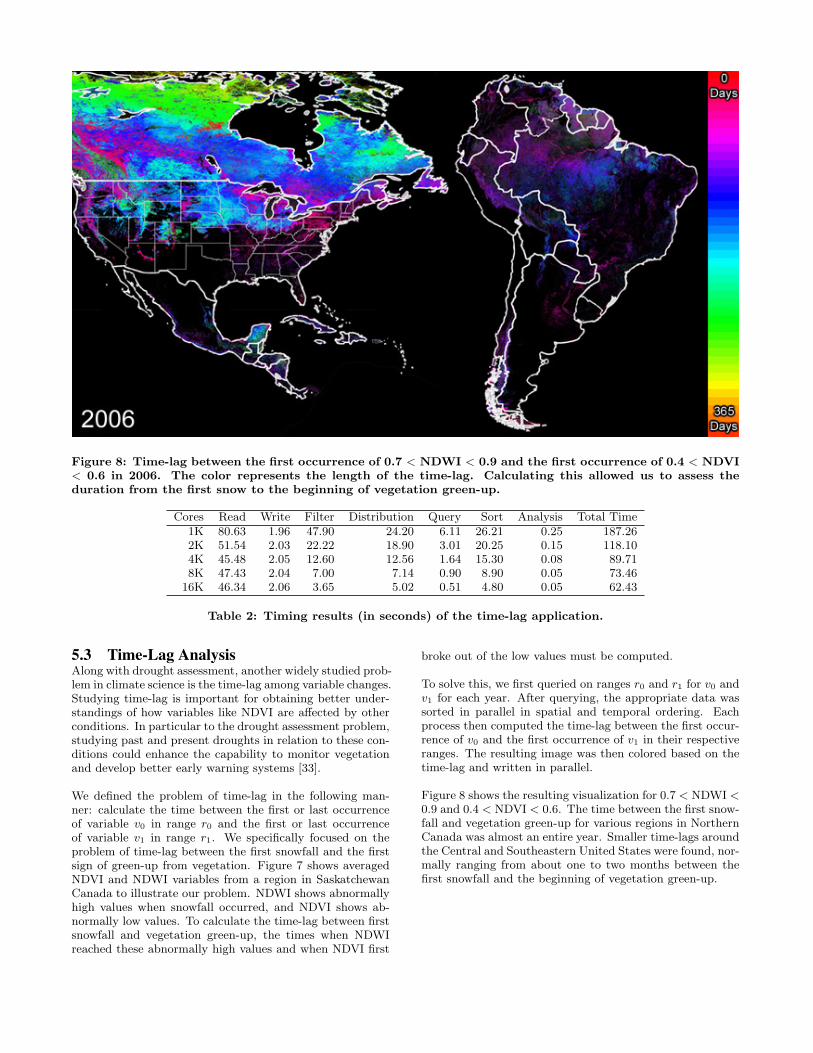
Figure 8: Time-lag between the first occurrence of 0.7 < NDWI < 0.9 and the first occurrence of 0.4 < NDVI< 0.6 in 2006. The color represents the length of the time-lag. Calculating this allowed us to assess theduration from the first snow to the beginning of vegetation green-up.

Cores Read Write Filter Distribution Query Sort Analysis Total Time1K 80.63 1.96 47.90 24.20 6.11 26.21 0.25 187.262K 51.54 2.03 22.22 18.90 3.01 20.25 0.15 118.104K 45.48 2.05 12.60 12.56 1.64 15.30 0.08 89.718K 47.43 2.04 7.00 7.14 0.90 8.90 0.05 73.46

16K 46.34 2.06 3.65 5.02 0.51 4.80 0.05 62.43

Table 2: Timing results (in seconds) of the time-lag application.

5.3 Time-Lag AnalysisAlong with drought assessment, another widely studied prob-lem in climate science is the time-lag among variable changes.Studying time-lag is important for obtaining better under-standings of how variables like NDVI are affected by otherconditions. In particular to the drought assessment problem,studying past and present droughts in relation to these con-ditions could enhance the capability to monitor vegetationand develop better early warning systems [33].

We defined the problem of time-lag in the following man-ner: calculate the time between the first or last occurrenceof variable v0 in range r0 and the first or last occurrenceof variable v1 in range r1. We specifically focused on theproblem of time-lag between the first snowfall and the firstsign of green-up from vegetation. Figure 7 shows averagedNDVI and NDWI variables from a region in SaskatchewanCanada to illustrate our problem. NDWI shows abnormallyhigh values when snowfall occurred, and NDVI shows ab-normally low values. To calculate the time-lag between firstsnowfall and vegetation green-up, the times when NDWIreached these abnormally high values and when NDVI first

broke out of the low values must be computed.

To solve this, we first queried on ranges r0 and r1 for v0 andv1 for each year. After querying, the appropriate data wassorted in parallel in spatial and temporal ordering. Eachprocess then computed the time-lag between the first occur-rence of v0 and the first occurrence of v1 in their respectiveranges. The resulting image was then colored based on thetime-lag and written in parallel.

Figure 8 shows the resulting visualization for 0.7 < NDWI <0.9 and 0.4 < NDVI < 0.6. The time between the first snow-fall and vegetation green-up for various regions in NorthernCanada was almost an entire year. Smaller time-lags aroundthe Central and Southeastern United States were found, nor-mally ranging from about one to two months between thefirst snowfall and the beginning of vegetation green-up.

0

0.2

0.4

0.6

0.8

1

0 20 40 60 80 100

Timestep

Time-Lag of First Snowfall and Vegetation Green-Up

NDVINDWI

22 Timesteps

21 Timesteps

Figure 7: Averaged NDVI and NDWI variables froma region in Saskatchewan Canada. Circled pointsshow the first occurrence of NDWI in the 0.7 – 0.9range and NDVI in the 0.4 – 0.6 range.

5.4 Application Timing ResultsTiming results were gathered from the two separate applica-tions. Detailed results of the drought application are shownin Table 1, and results from the time-lag application areshown in Table 2.

In the drought application, queries were issued on the grow-ing seasons of the Northern and Southern Hemispheres forall growing seasons, resulting in 18 total queries. One paral-lel sort was issued before analysis, and one final image waswritten. In Table 1, the aggregate time of all 18 queries isshown, along with timing for the other aspects of the appli-cation. With the parameters used to generate Figure 6, ≈11billion relevant items were returned from the queries andsorted before analysis. At 16K cores, the application aggre-gately queried ≈137.5 billion items per second and sorted≈2.6 billion items per second.

Similarly for the time-lag application, queries were issued foreach year on the Northern and Southern Hemispheres withthe beginning of each year starting in the Fall. For eachyear and hemisphere, a query was issued on the appropriaterange of NDVI and another was issued on the appropriaterange of NDWI to calculate time-lag. Thus, four querieswere issued each year. Since we were interested in time-lagon a yearly basis, we gathered the results separately for eachyear, resulting in 10 sorts being performed before analysisand 10 files being written.

The results in Table 2 show the aggregate times for thequerying, sorting, and writing, along with the times for theother parts of the application. With the parameters used togenerate Figure 8, ≈1.2 billion relevant items were returned,sorted, and analyzed for each year. Since we did this on all10 years, ≈12 billion relevant items were returned, sorted,and analyzed for the total application. At 16K cores, the ap-plication aggregately queried ≈23.5 billion items per secondand sorted ≈2.5 billion items per second.

Similar scaling results were observed in the applications.When scaling to 4K cores, I/O bandwidth reached≈25 GB/sbut then tapered off. This is because it was shown in [27]that using too many processes to perform I/O will oftencause bandwidth degradation. It is beyond the scope of ourwork right now to address this issue in our reading phase,however, we did gather the final image to a smaller amountof processes in the writing phase. This is why the writingtime remained near constant as process counts were scaled.

The aspects of the applications other than I/O showed scal-ability to 16K cores. The time for filtering the useless pointsin the dataset turned out to be a significant portion of theapplication, and more work will be needed to enable fasterfiltering of useless values. The analysis times were almostnegligible. When scaling to 16K cores, both applicationsshowed an end-to-end execution time of nearly one minute.

6. CONCLUSIONS AND FUTURE WORKIn this work we have shown the feasibility of performing so-phisticated, full-range analysis of terascale datasets directlyfrom application-native netCDF data. The end-to-end timefor these analyses can be optimized to about a minute, whichis acceptable to many scientific users. We have also sys-tematically evaluated a few common design alternatives inparallel reading of data as well as data distribution schemesfor load balancing. We found a greedily-driven assignmentof file reads to be a practical trade-off between complexityof I/O methods and achievable bandwidth. We have alsofound that, for terascale datasets handled by thousands ofcores, random distribution, while simplistic, actually demon-strated a trade-off advantage in user-perceived performance.

With this system and the small amount of time needed toperform queries, it is our future plan to study problems thatwill require many more queries to be issued. One exampleis a sensitivity-based study to determine which parametersare best for performing drought assessment, instead of givingstatic restrictions to the system. In addition, we also plan onextending our system to handle out-of-core datasets becausefuture growth of data will likely continue to outpace theincreases in system memory and processing bandwidth.

7. ACKNOWLEDGMENTSFunding for this work is primarily through the Institute ofUltra-Scale Visualization (http://www.ultravis.org) un-der the auspices of the SciDAC program within the U.S.Department of Energy (DOE). Important components of theoverall system were developed while supported in part by aDOE Early Career PI grant awarded to Jian Huang (No. DE-FG02-04ER25610) and by NSF grants CNS-0437508 andACI-0329323. The MODIS dataset was provided by NASA(http://modis.gsfc.nasa.gov). This research used resourcesof the National Center for Computational Science (NCCS)at Oak Ridge National Laboratory (ORNL), which is man-aged by UT-Battelle, LLC, for DOE under Contract No.DE-AC05-00OR22725.

8. REFERENCES[1] T. Peterka, H. Yu, R. Ross, and K.-L. Ma, “Parallel

volume rendering on the IBM Blue Gene/P,” inEGPGV ‘08: Proceedings of the EurographicsSymposium on Parallel Graphics and Visualization,April 2008, pp. 73–80.

[2] “MODIS,” http://modis.gsfc.nasa.gov.

[3] D. Silver and X. Wang, “Tracking and visualizingturbulent 3d features,” IEEE Transactions onVisualization and Computer Graphics, vol. 3, no. 2,pp. 129–141, 1997.

[4] W. E. Lorensen and H. E. Cline, “Marching cubes: Ahigh resolution 3d surface construction algorithm,” inProceedings of ACM SIGGRAPH, 1987, pp. 163–169.

[5] M. Glatter, C. Mollenhour, J. Huang, and J. Gao,“Scalable data servers for large multivariate volumevisualization,” IEEE Transactions on Visualizationand Computer Graphics, vol. 12, no. 5, pp. 1291–1298,2006.

[6] L. Gosink, J. C. Anderson, E. W. Bethel, and K. I.Joy, “Query-driven visualization of time-varyingadaptive mesh refinement data,” IEEE Transactionson Visualization and Computer Graphics, vol. 14,no. 6, 2008.

[7] K. Stockinger, J. Shalf, K. Wu, and E. Bethel,“Query-driven visualization of large data sets,” in VIS‘05: Proceedings of the IEEE VisualizationConference, October 2005, pp. 167–174.

[8] K.-L. Ma, C. Wang, H. Yu, and A. Tikhonova, “In situprocessing and visualization for ultrascalesimulations,” Journal of Physics, vol. 78, June 2007,(Proceedings of the SciDAC 2007 Conference).

[9] “Lustre,” http://www.lustre.org.

[10] W. Gropp, S. Huss-Lederman, A. Lumsdaine, E. Lusk,B. Nitzberg, W. Saphir, and M. Snir, MPI-TheComplete Reference: Volume 2 - The MPI Extensions.Cambridge, MA, USA: MIT Press, 1998.

[11] R. Thakur, W. Gropp, and E. Lusk, “Data sieving andcollective I/O in ROMIO,” in Proceedings of the 7thSymposium on the Frontiers of Massively ParallelComputation, 1999, pp. 182–189.

[12] K.-L. Ma, A. Stompel, J. Bielak, O. Ghattas, andE. J. Kim, “Visualizing large-scale earthquakesimulations,” in SC ‘03: Proceedings of theACM/IEEE Supercomputing Conference, 2003.

[13] H. Yu, K.-L. Ma, and J. Welling, “A parallelvisualization pipeline for terascale earthquakesimulations,” in SC ‘04: Proceedings of theACM/IEEE Supercomputing Conference, November2004.

[14] H. Yu, K.-L. Ma, and J. Welling, “I/O strategies forparallel rendering of large time-varying volume data,”in EGPGV ‘04: Proceedings of the EurographicsSymposium on Parallel Graphics and Visualization,June 2004, pp. 31–40.

[15] J. Lofstead, F. Zheng, S. Klasky, and K. Schwan,“Adaptable, metadata rich IO methods for portablehigh performance IO,” in IPDPS ‘09: Proceedings ofthe IEEE International Symposium on Parallel andDistributed Processing, 2009.

[16] M. Glatter, J. Huang, S. Ahern, J. Daniel, and A. Lu,“Visualizing temporal patterns in large multivariate

data using textual pattern matching,” IEEETransactions on Visualization and ComputerGraphics, vol. 14, no. 6, pp. 1467–1474, 2008.

[17] L. Gosink, J. Anderson, W. Bethel, and K. Joy,“Variable interactions in query-driven visualization,”IEEE Transactions on Visualization and ComputerGraphics, vol. 13, no. 6, pp. 1400–1407, 2007.

[18] K. Stockinger, E. W. Bethel, S. Campbell, E. Dart,and K. Wu, “Detecting distributed scans usinghigh-performance query-driven visualization,” in SC‘06: Proceedings of the ACM/IEEE SupercomputingConference, October 2006.

[19] O. Rubel, Prabhat, K. Wu, H. Childs, J. Meredith,C. G. R. Geddes, E. Cormier-Michel, S. Ahern, G. H.Weber, P. Messmer, H. Hagen, B. Hamann, and E. W.Bethel, “High performance multivariate visual dataexploration for extremely large data,” in SC ‘08:Proceedings of the ACM/IEEE SupercomputingConference, November 2008.

[20] G. E. Blelloch, C. E. Leiserson, B. M. Maggs, C. G.Plaxton, S. Smith, and M. Zagha, “An experimentalanalysis of parallel sorting algorithms,” Theory ofComputing Systems, vol. 31, no. 2, pp. 135–167, 1998.

[21] M. Meissner, J. Huang, D. Bartz, K. Mueller, andR. Crawfis, “A practical evaluation of the four mostpopular volume rendering algorithms,” in Proceedingsof the IEEE/ACM Symposium on VolumeVisualization, October 2000.

[22] F.-Y. Tzeng and K.-L. Ma, “Intelligent featureextraction and tracking for visualizing large-scale 4dflow simulations,” in SC ‘05: Proceedings of theACM/IEEE Supercomputing Conference, November2005.

[23] R. Ross, T. Peterka, H.-W. Shen, K.-L. Ma, H. Yu,and K. Moreland, “Visualization and parallel I/O atextreme scale,” Journal of Physics, vol. 125, July 2008,(Proceedings of the SciDAC 2008 Conference).

[24] R. Rew and G. Davis, “NetCDF: An interface forscientific data access,” IEEE Computer Graphics andApplications, vol. 10, no. 4, pp. 76–82, 1990.

[25] J. Li, W. Liao, A. Choudhary, R. Ross, R. Thakur,W. Gropp, R. Latham, A. Siegel, B. Gallagher, andM. Zingale, “Parallel netCDF: A high-performancescientific I/O interface,” in SC ‘03: Proceedings of theACM/IEEE Supercomputing Conference, 2003.

[26] G. Memik, M. T. Kandemir, W.-K. Liao, andA. Choudhary, “Multicollective I/O: A technique forexploiting inter-file access patterns,” ACMTransactions on Storage, vol. 2, no. 3, pp. 349–369,2006.

[27] W. Yu, J. S. Vetter, and S. Oral, “Performancecharacterization and optimization of parallel I/O onthe Cray XT,” in IPDPS ‘08: Proceedings of the IEEEInternational Symposium on Parallel and DistributedProcessing, 2008, pp. 1–11.

[28] “IOR,”http://www.cs.sandia.gov/Scalable IO/ior.html.

[29] Y. Gu, J. F. Brown, J. P. Verdin, and B. Wardlow, “Afive-year analysis of MODIS NDVI and NDWI forgrassland drought assessment over the Central GreatPlains of the United States,” Geophysical ResearchLetters, vol. 34, 2007.

[30] B. Gao, “NDWI – A normalized difference water indexfor remote sensing of vegetation liquid water fromspace,” Remote Sensing of Environment, vol. 58, no. 3,pp. 257–266, December 1996.

[31] L. Wang, J. Qu, and X. Xiong, “A seven year analysisof water related indices for Georgia droughtassessment over the 2007 wildfire regions,” IEEEInternational Geoscience and Remote SensingSymposium, 2008.

[32] C. Liu and J. Wu, “Crop drought monitoring usingMODIS NDDI over mid-territory of China,” IEEEInternational Geoscience and Remote SensingSymposium, 2008.

[33] T. Tadessee, B. D. Wardlow, and J. H. Ryu,“Identifying time-lag relationships between vegetationcondition and climate to produce vegetation outlookmaps and monitor drought,” 22nd Conference onHydrology, 2008.