Tensor Product Surfaces Guided by Minimal Surface Area Triangulations

John K. Johnstone∗and Kenneth R. Sloan

Department of Computer and Information SciencesUniversity of Alabama at Birmingham

115A Campbell Hall, 1300 University BoulevardBirmingham, Alabama 35294-1170 USA{johnstone,sloan}@cis.uab.edu

http://www.cis.uab.edu/

AbstractWe present a method for constructing tensor product

Bezier surfaces from contour (cross-section) data. Mini-mal area triangulations are used to guide the surface con-struction, and the final surface reflects the optimality of thetriangulation. The resulting surface differs from the initialtriangulation in two important ways: it is smooth (as op-posed to the piecewise planar triangulation), and it is intensor product form (as opposed to the irregular triangu-lar mesh). The surface reconstruction is efficient becausewe do not require an exact minimal surface. The triangu-lations are used as strong hints, but no more than that.

The method requires the computation of both open andclosed isoparametric curves of the surface, using triangu-lations as a guide. These isoparametric curves form a ten-sor product Bezier surface. We show how to control sam-pling density by filling and pruning isoparametric curves,for accuracy and economy.

A rectangular grid of points is produced that is compat-ible with the expected format for a tensor product surfaceinterpolation, so that a host of well-supported methods areavailable to generate and manipulate the surface.

Keywords: surface reconstruction, contour data, mini-mum area triangulation, Bezier surface, biomedical visual-ization

1 IntroductionThe classical reconstruction problem of finding a sur-

face from polygons extracted from serial sections is im-portant to several disciplines. A common application isreconstruction of slices of MRI or CT data (Figure 4), aswell as slice data from industrial and geophysical imaging.The conventional way to reconstruct this data into a sur-face is by an optimal triangulation, classically a minimum-

∗This work partially supported by National Science Foundation grantCCR-9213918.

area triangulation [3] (see Figure 5). This clearly creates apolyhedral approximation to the surface. A smooth surfacereconstruction has advantages over a triangulation, just aspiecewise cubic curve fitting of point data has advantagesover piecewise linear fitting.1 If the interslice distance isvery small and each slice is densely sampled, then a tri-angulation is fully adequate; however, this is often not thecase.2

It is infeasible to exactly find a minimal area smoothsurface reconstruction to the polygonal data.3 The beautyof a triangulation is that there are only a finite number ofvalid triangulations, and so it is tractable to find the opti-mal one. Our approach, therefore, is to use the triangu-lar reconstruction to guide the smooth surface reconstruc-tion. In essence, we view the optimal triangulation as adiscrete approximation to the optimal surface reconstruc-tion that needs only be refined. This approach also allowsus to tap into previous work on triangular reconstruction ofslice data, rather than abandoning it.

In this paper, we use the widely accepted optimality cri-terion of minimum area. To repeat, rather than computinga minimal surface exactly, we use the minimum-area trian-gulation to guide us to a smooth surface that is consistentwith the minimum-area triangulation and thus a good ap-proximation to a minimal surface interpolating the data.

We choose the rational Bezier surface as our smoothsurface, for reasons of efficiency and compatibility, and forall of the well-known advantages of Bezier surfaces [2].More specifically, we choose the tensor product rational

1Just as a line is not usually the best approximation to the shape of acurve between two points, a triangle is not usually the best approximationto the shape of a surface between three points (especially the shape of ahuman organ).

2Slices are spaced out due to concerns about radiation exposure, limi-tations in technology, limitations in time, and other factors.

3Moreover, this surface may not be desirable as precisely minimalsurfaces can adopt strange shapes.

Bezier surface. However, in order to interpolate a point setby a tensor product surface, the points should be organizedinto rows and columns of a rectangular grid. Moreover, thepoints in each row (resp., column) of the grid will be placedon the same isoparametric curve of the surface.4 Once wehave a rectangular grid of data points in this conventionalformat, there are a host of well-supported ways of generat-ing and manipulating the surface.

Therefore, our problem reduces to finding naturalisoparametric curves defined by the original slice data, inorthogonal directions (or actually, just a set of points onthese isoparametric curves). The basic step in our methodis to choose a curve which spans the surface in one direc-tion, place ’seed points’ along this curve, and allow theseseeds to ’flow’ in the orthogonal direction. The flow of asingle seed point defines a curve. The flow of the ensembleof seed points defines a set of isoparametric curves whichare orthogonal to the originally chosen curve.

The following argument establishes why it is valid touse the triangulation to find a point on the same isopara-metric curve. As the number of points on each slice in-creases, the triangles of the minimum-area triangulationbecome thinner, and in the limit become lines connectingtwo points on neighbouring slices. Notice that, in this limitcase, each point on slicei is connected to just one point onslice i + 1. That is, this limit surface is a lofting betweenthe two slices.

Definition 1 A lofting of two curvesc(t) and d(t) is thesurface generated by joining each pair of points with thesame parameter value by a straight line, which becomesan isoparametric curve of the surface.

Moreover, this is a minimum-area lofting since it is gen-erated by the limit of minimum-area triangulations. Inother words, a minimum-area triangulation can be viewedas a discrete approximation to a minimum-area lofting. Buta minimum-area lofting is itself a linear approximation tothe minimal-area surface connecting the two slices, the sur-face that we are striving for (but willing to approximatesmoothly). That is, the straight lines of the lofting arelinear approximations to the isoparametric curves of theminimal surface. Thus, a minimum-area triangulation is adiscrete approximation to a linear approximation of a min-imal surface; and a triangle of a minimum-area triangula-tion is a discrete approximation to a linear approximationof an isoparametric curve of the minimal surface. The tri-angles of the minimum-area triangulation should thereforebe used as guides to the isoparametric curves of the smoothsurface reconstruction.

4This is due to the fact that the rows and columns of a tensor productcontrol mesh are associated with isoparametric curves of the surface [2].

We will refer to the process of following the triangula-tion to find isoparametric curves as ‘flowing over the trian-gulation’ and the isoparametric curves that we find as ‘flowlines’. We purposefully use the term ‘flow’ to describe thisprocess, since the flow of isoparametric curves across theminimal triangulation behaves quite similarly to the flowof liquid across a surface. However, we are not using tra-ditional methods of flow computation.

Here is a high-level sketch of the method:

• Triangulate the original ’horizontal’ contour data.

• Place seed points along a central cross-section andflow these points to form a collection of isoparamet-ric (piecewise linear) curves orthogonal to the cross-sections.

• Triangulate these ’vertical’ curves.

• Place seed points along one ’vertical’ curve and flowthese points to form a collection of isoparametriccurves (’horizontal’ again!).

At each stage, care must be taken to ensure that the ap-proximations are adequate. The number and spacing of the’seed points’ are adjusted, as needed.

The rest of the paper is structured as follows. In Sec-tion 2, we place this paper in the perspective of previ-ous work on surface reconstruction from slices. In Sec-tion 3, we formalize how to use the triangulation to com-pute isoparametric curves of the surface reconstruction. InSection 4, we show how to place the isoparametric curvesin order to properly cover the surface. In Section 5, weshow how the computation of closed isoparametric curvesdiffers from the computation of open isoparametric curves.In Section 6, we recall how a tensor product surface can beconstructed from the isoparametric curves, or rather froma grid of points on isoparametric curves. We review andaccumulate the steps of the entire reconstruction algorithmin Section 7, and we end with some conclusions.

Note that in this paper we have chosen a very restrictedclass of surfaces, namely those which are easily and natu-rally described by a tensor product Bezier mesh. Essen-tially, this limits us to surfaces which are topologicallyequivalent to a cylinder. Branching structures are beyondthe scope of this work (but see [6]). We can easily adaptour method to the reconstruction of surfaces with the topol-ogy of a sheet or torus. For surfaces with the topology of acylinder, we must already deal with both open and closedisoparametric curves. With the torus, both sets of isopara-metric curves are closed, and with the sheet they are bothopen.

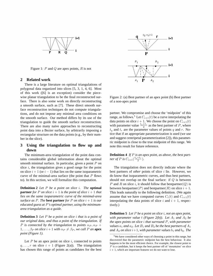
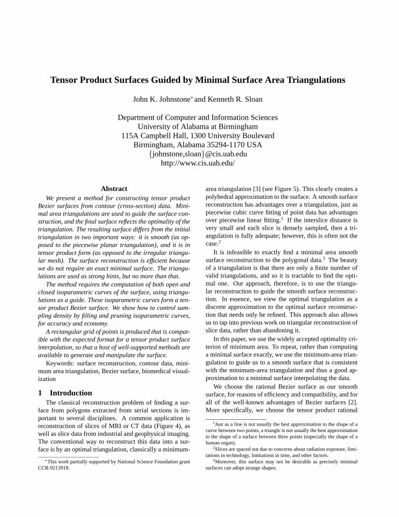
Figure 1:P andQ are apex points,R is not

2 Related workThere is a large literature on optimal triangulations of

polygonal data organized into slices [5, 3, 1, 4, 6]. Mostof this work ([6] is an exception) consider the piece-wise planar triangulation to be the final reconstructed sur-face. There is also some work on directly reconstructinga smooth surface, such as [7]. These direct smooth sur-face reconstruction techniques do not compute triangula-tions, and do not impose any minimal area conditions onthe smooth surface. Our method differs by its use of thetriangulation to guide the smooth surface reconstruction.There are also many naive approaches to reconstructingpoint data into a Bezier surface, by arbitrarily imposing arectangular structure on the data points (e.g., by their num-ber in the slice).

3 Using the triangulation to flow up anddown

The minimum-area triangulation of the point data con-tains considerable global information about the optimalsmooth minimal surface. In particular, given a pointP onslice i, the triangulation gives a good range for the pointon slicei+ 1 (or i− 1) that lies on the same isoparametriccurve of the minimal-area surface (the point thatP flowsto). In this section, we will formalize this computation.

Definition 2 Let P be a point on slicei. The optimalpartner for P on slicei+ 1 is the point of slicei+ 1 thatlies on the same isoparametric curve of the minimal-areasurface asP . Thebest partner for P on slicei+ 1 is oureducated guess atP ’s optimal partner, using the minimum-area triangulation as a guide.

Definition 3 LetP be a point on slicei that is a point ofour original data, and thus a point of the triangulation. IfP is connected by the triangulation to pointsαP , αP +1, . . . , βP on slicei+ 1 withαP 6= βP , we callP anapexpoint (Figure 1).

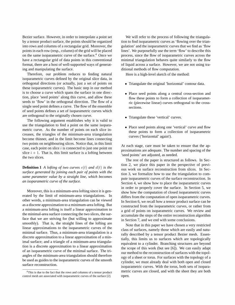
Let P be an apex point on slicei, connected to pointsq, . . . , r on slice i + 1 (Figure 2(a)). The triangulationhas chosen this range of points as candidates for the best

Figure 2: (a) Best partner of an apex point (b) Best partnerof a non-apex point

partner. We compromise and choose the ‘midpoint’ of thisrange, as follows.5 LetCi+1(t) be a curve interpolating thedata points on slicei+ 1. We choose the point onCi+1(t)with parameter valuetq+tr2 as the best partner ofP , wheretq andtr are the parameter values of pointsq andr. No-tice that if an appropriate parameterization is used (we useand suggest centripetal parameterization [2]), this paramet-ric midpoint is close to the true midpoint of this range. Wenote this result for future reference.

Definition 4 If P is an apex point, as above, the best part-ner ofP isCi+1( tq+tr2 ).

The triangulation does not directly indicate where thebest partners ofother points of slicei lie. However, wedo know that isoparametric curves, and thus best partners,should not overlap on the final surface: ifQ is betweenP andR on slicei, it should follow that bestpartner(Q) isbetween bestpartner(P ) and bestpartner(R) on slicei+ 1.This leads naturally to the following definition. (We againassume that we have computed curvesCi(t) andCi+1(t)interpolating the data points of slicei and i + 1, respec-tively.)

Definition 5 LetP be a point on slicei, not an apex point,with parameter valuet (Figure 2(b)). LetA1 andA2 bethe apex points on slicei that surroundP , with parametervaluesa1 anda2. LetB1 andB2 be the best partners ofA1

andA2 on slicei+1, with parameter valuesb1 andb2. The

5We have considered other ways of choosing a point in this range, butdiscovered that the parametric midpoint has the best behaviour. It alsohappens to be the most efficient choice. For example, the closest point toP is a candidate, but it keeps the best partner off of ‘mountains’ on slicei+ 1, which are important features we do not want to lose.

best partner ofP is the point on_

B1B2 in the same ratio

asP on the segment_

A1A2: i.e., the point with parametervalue a2−t

a2−a1∗ b1 + t−a1

a2−a1∗ b2.

This establishes how the triangulation guides the flow ofpoints to neighbouring slices. We have restricted our dis-cussion to upward flow, from slicei to slicei + 1: down-ward flow from slicei to slicei− 1 is entirely analogous.

The reader will have noticed that we have made heavyuse of interpolating curves in the computation of best part-ners. In effect, on each slicei, the original data consistingof ni points has been replaced by a smooth curve6 that in-terpolates this data. This is consistent with our goal of gen-erating a smooth surface: a triangulated surface implicitlyrepresents each slice by the polygon connecting the datapoints; a smoother curve is a better representation for theslice (especially for biomedical objects).

4 Seeding flow lines4.1 Original seeds

We are now ready to create isoparametric curves of oursurface (Figure 7). In the following, isoparametric curveswill be referred to as flow lines. We begin with ‘vertical’isoparametric curves (if slices are horizontal).

We start with a data point (a ‘seed’) and flow it to allother slices. Suppose there aren slices. IfPi is our originalseed on slicei, we computePj for i < j < n wherePj isthe best partner ofPj−1 (flowing up) and then we computePj for 0 ≤ j < i wherePj is the best partner ofPj+1

(flowing down). The set{Pj : 0 ≤ j < n} is a discreterepresentation of an isoparametric curve of the surface.

Initially, we choose seed points on only one of theslices.7 We now explain why this is not enough.

4.2 MountainsConsider Figure 3. It shows a tall feature on one slice.

These tall features are commonly connected to only onepoint on a neighbouring slice by the minimum-area trian-gulation, as shown.

Definition 6 A mountain is a segmentS of a slice suchthat the data points onS are all connected by the trian-gulation to a single pointQ on a neighbouring slice (Fig-ure 3). IfP andR are the data points neighbouringQ, the

segment_

PR is called thepassinto the mountain.

An interesting characteristic of the flow procedure of theprevious section is that it tends to avoid mountains. This isdue to the narrow passes onto mountains. In Figure 3, the

6We use cubic B-splines.7We choose the middle slice in our implementation. Any one of the

slices is a good choice and delivers similar results, except for the first andlast slices which are often degenerate.

Figure 3: A mountain_

AB

only way for a flow line to travel over the mountain_

AB is

for the flow line to enter slicei in the segment_

PR, a nar-row pass that always contains just three data points. How-ever, notice that it is very unfortunate to miss the moun-tains, since the mountains of our data set contain all of theinteresting features: without mountains, each slice is es-sentially flat. So to represent a tensor product surface bya network of curves that remains in the valleys and rarelyventures onto the mountains is a mistake. We thereforeseed the mountains as well.

Rather than identifying mountains by their above defi-nition, we recognize them as features not yet captured bythe flow lines. Consider a slice and the flow lines that crossit, say at pointsF1, . . . , Fm. Consider a data pointP on

this slice that lies on segment_

FjFj+1. If the distance of

P from the line↔

FjFj+1 is greater than some user-definedvalued, then we seed another flow line fromP . The valueof d allows the designer to control the feature size that willbe captured by the surface, and thus the accuracy of thereconstruction. This process of looking for ‘mountains’and seeding them is done repeatedly on each slice untilall mountains are covered by flow lines. Our experienceshows that there are only a few mountains that need to beseeded in any data set (11 in the example of Figure 7).

Notice that the number of original seeds chosen in Sec-tion 4.1 is not critical: we may start with only a few andthen rely upon the seeding of mountains as above. We cer-tainly do not need to place a seed at every data point inSection 4.1.

4.3 Flowing from mountainsThe computation of best partners during the seeding

of mountains is slightly different than during our originalseeding. In the original seeding, the flow line is guidedonly by the triangulation. However, we are now insert-ing a flow line in between two existing flow lines, so thenew flow line must also be guided by these flow lines, toavoid crossing neighbouring flow lines. Consider a newseed pointP on slicei that lies between flow linesF1 andF2, and suppose that we want to compute its best partner on

slicei+ 1. The triangulation suggests that the best partner

lies somewhere in the range_

AB8 while the flow lines en-force that it must lie between flow linesF1 andF2. To findthe best partner, we intersect these two ranges. If they donot overlap (which occurs only rarely), the flow line rangetakes precedence. Within this new range, we choose theexact position of the best partner by straightforward linearinterpolation based on the position of the original pointPwithin the associated interval on slicei.

4.4 Pruning flow linesDuring the construction of flow lines, it is possible for

two flow lines to come undesirably close (based on someuser-defined measure), although they will never cross. Thiscommonly occurs if the triangulation and flow lines con-spire to force two newly introduced flow lines through avery thin pass. It is simple to identify this occurence9 and itcan be corrected as follows. Suppose that flow linesA andB come undesirably close. At present, a flow line is onlydefined byn points, one per slice. Let then points of flowlineA beP1, . . . , Pn with parameter valuess1, . . . , sn ontheir respective slices. Let then points of flow lineB beQ1, . . . , Qn with parameter valuest1, . . . , tn. We createthe average of the two flow lines, defined by then pointswith parameter valuess1+t1

2 , . . . , sn+tn2 on slices1, . . . , n,

respectively. We then remove flow linesA andB and re-place them by the average flow line.

5 Flowing in the orthogonal directionWe do not yet have the desired grid of points to con-

struct a tensor product surface. At present we have a setof isoparametric curves (Figure 7) and we known pointson each of these isoparametric curves (the points wherethese isoparametric curves cross the slices). Suppose thatwe havem isoparametric curves and then points on thejth isoparametric curve arep1,j , p2,j , . . . , pn,j (wherepi,jlies on slicei). Suppose that we create a rectangular grid ofthese points,{pi,j}. The points of the columns of this gridlie on isoparametric curves, as desired, but unfortunatelythe points of the rows do not: the points of rowi are shack-led to slicei, and slicei is not necessarily an isoparametriccurve. We want to allow the points in theith row to strayfrom the slices to achieve a better surface.

Luckily we have almost all of the weaponry to achievethis: we merely interpret the flow lines we have constructedas new slices and repeat the above procedure. That is, weconstruct the minimum-area triangulation of the new slicesand use the triangulation to guide the construction of new

8For example, ifP lies between the two apex pointsA1 andA2, thenthe range for the best partner ofP is between the best partner ofA1 andthe best partner ofA2.

9We have found it rarely necessary to prune flow lines in this way ifseeds are chosen properly.

flow lines. This will create isoparametric curves in the or-thogonal direction.

The second triangulation will be somewhat faster be-cause it is open rather than closed (O(n2) rather thanO(n2 log n)). It is also better-conditioned than the first,but we do not use this to speed up the triangulation (e.g.,by using a band-box triangulation) since we still want theminimum-area triangulation. The whole algorithm can beviewed as improving the quality of the data (for the pur-poses of tensor product surface interpolation) and the finaldata would be yet easier to triangulate.

There is only one problem: the original isoparametriccurves that we created were open, while the new isopara-metric curves we will be creating must be closed (Fig-ure 10). There is no guarantee that if we flow out frompointP on slice 1, using the triangulation to guide us, thatthis flow will return to slice 1 at the same pointP after itwraps around. To enforce the creation of closed flow lines,we use the following variation on finding the best partner.

Definition 7 From any slice, we can flow in two directions,since the slices form a closed loop. We want to flow inboth directions and compromise. Letp be a seed point onisoparametric curve 1. Suppose that pointsqL andqR onisoparametric curvei are found by flowing left and rightfromP , with parameter valuestL andtR. Then we choosethe point with parameter valuetL+tR

2 as the best partnerof P on isoparametric curvei.

6 Construction of the tensor product Beziercontrol mesh

Our goal in producing a rectangular grid of points wasto create an input compatible with the expected format fora tensor product surface interpolation. Once we have apoint set in this conventional format, there are a host ofwell-supported ways of generating and manipulating thesurface.

The construction of a tensor product (Bezier or B-spline) interpolant is classical (see Farin [2]). As part ofthe construction, the points of a row (resp., column) of therectangular grid define an isoparametric curve of the sur-face.

7 The algorithm in reviewWe now review the entire reconstruction algorithm. The

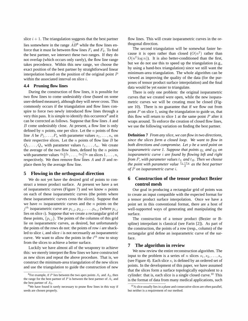
input to the problem is a series ofn slicess1, s2, . . . , sn(see Figure 4). Each slicesi is defined by an ordered set ofpoints. In the development of this paper, we have assumedthat the slices form a surface topologically equivalent to acylinder: that is, each slice is a single closed curve.10 Thisis the format of data from many medical applications, such

10A slice usually lies in a plane and consecutive slices are often parallel,but neither is a requirement of our method.

as the crucial areas of cardiology and neurosurgery. How-ever, the same techniques can be used for surfaces topolog-ically equivalent to a plane or a torus, since we show howto deal with both open and closed isoparametric curves.

1. (Interpolate and resample.)On each slicesi, interpo-late the points of the slice by a smooth rational curveCi (e.g., a cubic Bezier spline). This becomes the newrepresentation for the slice.

We assume that the original point data is well sampledon the slices (as it is in our examples). If it is not,it should be resampled fromCi. Resampling can beused to correct either over- or under-sampling in theoriginal data.

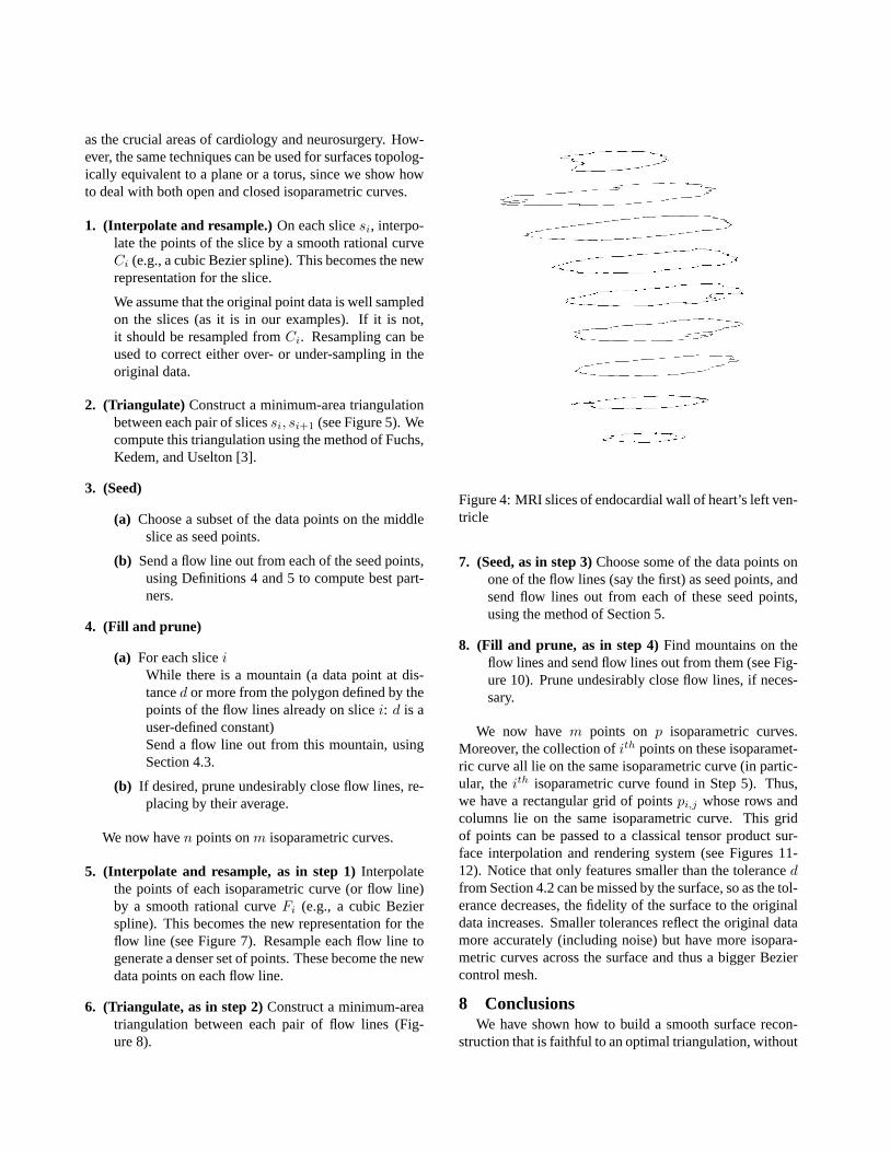
2. (Triangulate) Construct a minimum-area triangulationbetween each pair of slicessi, si+1 (see Figure 5). Wecompute this triangulation using the method of Fuchs,Kedem, and Uselton [3].

3. (Seed)

(a) Choose a subset of the data points on the middleslice as seed points.

(b) Send a flow line out from each of the seed points,using Definitions 4 and 5 to compute best part-ners.

4. (Fill and prune)

(a) For each sliceiWhile there is a mountain (a data point at dis-tanced or more from the polygon defined by thepoints of the flow lines already on slicei: d is auser-defined constant)Send a flow line out from this mountain, usingSection 4.3.

(b) If desired, prune undesirably close flow lines, re-placing by their average.

We now haven points onm isoparametric curves.

5. (Interpolate and resample, as in step 1)Interpolatethe points of each isoparametric curve (or flow line)by a smooth rational curveFi (e.g., a cubic Bezierspline). This becomes the new representation for theflow line (see Figure 7). Resample each flow line togenerate a denser set of points. These become the newdata points on each flow line.

6. (Triangulate, as in step 2)Construct a minimum-areatriangulation between each pair of flow lines (Fig-ure 8).

Figure 4: MRI slices of endocardial wall of heart’s left ven-tricle

7. (Seed, as in step 3)Choose some of the data points onone of the flow lines (say the first) as seed points, andsend flow lines out from each of these seed points,using the method of Section 5.

8. (Fill and prune, as in step 4)Find mountains on theflow lines and send flow lines out from them (see Fig-ure 10). Prune undesirably close flow lines, if neces-sary.

We now havem points on p isoparametric curves.Moreover, the collection ofith points on these isoparamet-ric curve all lie on the same isoparametric curve (in partic-ular, theith isoparametric curve found in Step 5). Thus,we have a rectangular grid of pointspi,j whose rows andcolumns lie on the same isoparametric curve. This gridof points can be passed to a classical tensor product sur-face interpolation and rendering system (see Figures 11-12). Notice that only features smaller than the tolerancedfrom Section 4.2 can be missed by the surface, so as the tol-erance decreases, the fidelity of the surface to the originaldata increases. Smaller tolerances reflect the original datamore accurately (including noise) but have more isopara-metric curves across the surface and thus a bigger Beziercontrol mesh.

8 ConclusionsWe have shown how to build a smooth surface recon-

struction that is faithful to an optimal triangulation, without

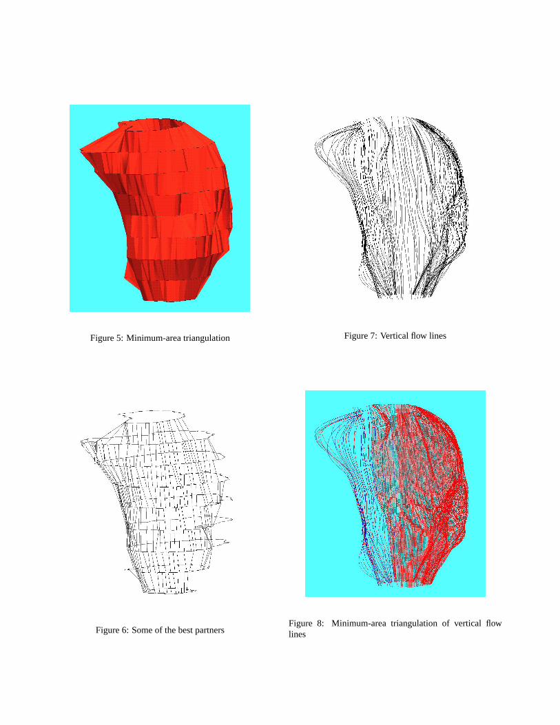
Figure 5: Minimum-area triangulation

Figure 6: Some of the best partners

Figure 7: Vertical flow lines

Figure 8: Minimum-area triangulation of vertical flowlines

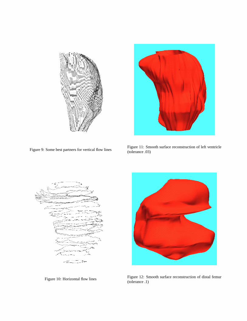
Figure 9: Some best partners for vertical flow lines

Figure 10: Horizontal flow lines

Figure 11: Smooth surface reconstruction of left ventricle(tolerance .03)

Figure 12: Smooth surface reconstruction of distal femur(tolerance .1)

the intolerable expense of computing a truly optimal sur-face. Although we approximate the given data by the sur-face, the accuracy of the surface to the original point datacan be controlled by the designer. A characteristic of ourmethod is that each step discards previous data: we startwith original slices, move to vertical flow lines, and thenhorizontal flow lines, which finally define the input to thetensor product interpolation. Finally, we have addressedthe issue of sampling density by filling and pruning flowlines, for accuracy, economy, and numerical stability.

In this paper, we have used the term ‘minimal area tri-angulation’. It turns out that it is not always sufficient tosimply minimize the area. In certain pathological cases(which are beyond the scope of this paper), it is necessaryto consider not only the area, but also the aspect ratio of in-dividual triangles. Briefly, we achieve this by consideringboth the area and the perimeter of each triangle. The effectis to generate a minimal area surface almost everywhere–the perimeter information simply breaks ties between com-peting triangulations with very similar surface area.

AcknowledgementsWe thank the UAB NMR Lab, Ross Singleton, and Ger-

ald Blackwell for the MRI data of the left ventricle, andAlan Eberhardt and Peter Czuwala for the MRI data of thedistal femur.

References[1] Christiansen, H.H. and T.W. Sederberg (1978) Conver-

sion of complex contour line definitions into polygonalelement mosaics. Computer Graphics, XIII, 2, August.

[2] Farin, G. (1993) Curves and surfaces for computeraided geometric design. Academic Press (New York),third edition.

[3] Fuchs, H., Z. Kedem, and S. Uselton (1977) Optimalsurface reconstruction from planar contours. Commu-nications of the ACM, 20:10, October, 693–702.

[4] Ganapathy, S. and T.G. Dennehy (1982) A new gen-eral triangulation method for planar contours. Com-puter Graphics, Vol. 16, No. 3, July.

[5] Keppel, E. (1975) Approximating complex surfaces bytriangulation of contour lines. IBM J. Res. Develop.19, January.

[6] Meyers, D., S. Skinner, and K. Sloan (1992) Surfacesfrom contours. ACM Transactions on Graphics, Vol.11, No. 3, July, pp. 228-258.

[7] Wu, S.-C., J.F. Abel, and D.P. Greenberg (1977) Aninteractive computer graphics approach to surface rep-resentation. Communications of the ACM, Vol. 20, No.10, October, pp. 703–712.