techniques of integration - wordpress.com · techniques of integration the techniques of this...
TRANSCRIPT

Techniques of Integration
The techniques of this
chapter enable us to find
the height of a rocket a
minute after liftoff and to
compute the escape
velocity of the rocket.

Because of the Fundamental Theorem of Calculus, we can
integrate a function if we know an antiderivative, that is,
an indefinite integral. We summarize here the most impor-
tant integrals that we have learned so far.
In this chapter we develop techniques for using these basic integration formulas
to obtain indefinite integrals of more complicated functions. We learned the most
important method of integration, the Substitution Rule, in Section 5.5. The other gen-
eral technique, integration by parts, is presented in Section 7.1. Then we learn
methods that are special to particular classes of functions such as trigonometric func-
tions and rational functions.
Integration is not as straightforward as differentiation; there are no rules that
absolutely guarantee obtaining an indefinite integral of a function. Therefore, in
Section 7.5 we discuss a strategy for integration.
|||| 7.1 I n t e g r a t i o n b y P a r t s
Every differentiation rule has a corresponding integration rule. For instance, the Substi-tution Rule for integration corresponds to the Chain Rule for differentiation. The rule thatcorresponds to the Product Rule for differentiation is called the rule for integration byparts.
The Product Rule states that if and are differentiable functions, then
d
dx � f �x�t�x�� � f �x�t��x� � t�x�f ��x�
tf
y 1
sa 2 � x 2 dx � sin�1� x
a� � Cy 1
x 2 � a 2 dx �1
a tan�1� x
a� � C
y cot x dx � ln � sin x � � Cy tan x dx � ln � sec x � � C
y cosh x dx � sinh x � Cy sinh x dx � cosh x � C
y csc x cot x dx � �csc x � Cy sec x tan x dx � sec x � C
y csc2x dx � �cot x � Cy sec2x dx � tan x � C
y cos x dx � sin x � Cy sin x dx � �cos x � C
y ax dx �ax
ln a� Cy ex dx � ex � C
y 1
x dx � ln � x � � C�n � �1�y xn dx �
xn�1
n � 1� C

476 ❙ ❙ ❙ ❙ CHAPTER 7 TECHNIQUES OF INTEGRATION
In the notation for indefinite integrals this equation becomes
or
We can rearrange this equation as
Formula 1 is called the formula for integration by parts. It is perhaps easier to remem-ber in the following notation. Let and . Then the differentials are
and , so, by the Substitution Rule, the formula for integrationby parts becomes
EXAMPLE 1 Find .
SOLUTION USING FORMULA 1 Suppose we choose and . Then and . (For we can choose any antiderivative of .) Thus, using Formula1, we have
It’s wise to check the answer by differentiating it. If we do so, we get , asexpected.
SOLUTION USING FORMULA 2 Let
Then
and so
� �x cos x � sin x � C
� �x cos x � y cos x dx
y x sin x dx � y x sin x dx � x ��cos x� � y ��cos x� dx
v � �cos x du � dx
dv � sin x dx u � x
x sin x
� �x cos x � sin x � C
� �x cos x � y cos x dx
� x��cos x� � y ��cos x� dx
y x sin x dx � f �x�t�x� � y t�x�f ��x� dx
t�tt�x� � �cos xf ��x� � 1t��x� � sin xf �x� � x
y x sin x dx
y u dv � uv � y v du2
dv � t��x� dxdu � f ��x� dxv � t�x�u � f �x�
y f �x�t��x� dx � f �x�t�x� � y t�x�f ��x� dx1
y f �x�t��x� dx � y t�x�f ��x� dx � f �x�t�x�
y � f �x�t��x� � t�x�f ��x�� dx � f �x�t�x�
u d√ u √ √ du
|||| It is helpful to use the pattern:
v � � du � �
dv � � u � �

SECTION 7.1 INTEGRATION BY PARTS ❙ ❙ ❙ ❙ 477
NOTE ■■ Our aim in using integration by parts is to obtain a simpler integral than the onewe started with. Thus, in Example 1 we started with and expressed it in termsof the simpler integral . If we had chosen and , then
and , so integration by parts gives
Although this is true, is a more difficult integral than the one we started with.In general, when deciding on a choice for and , we usually try to choose tobe a function that becomes simpler when differentiated (or at least not more complicated)as long as can be readily integrated to give .
EXAMPLE 2 Evaluate .
SOLUTION Here we don’t have much choice for and . Let
Then
Integrating by parts, we get
Integration by parts is effective in this example because the derivative of the functionis simpler than .
EXAMPLE 3 Find .
SOLUTION Notice that becomes simpler when differentiated (whereas is unchangedwhen differentiated or integrated), so we choose
Then
Integration by parts gives
The integral that we obtained, , is simpler than the original integral but is still notobvious. Therefore, we use integration by parts a second time, this time with and u � t
x tet dt
y t 2et dt � t 2et � 2 y tet dt3
du � 2t dt v � et
u � t 2 dv � et dt
ett 2
y t 2et dt
ff �x� � ln x
� x ln x � x � C
� x ln x � y dx
y ln x dx � x ln x � y x dx
x
du �1
x dx v � x
u � ln x dv � dx
dvu
y ln x dx
vdv � t��x� dx
u � f �x�dvux x 2 cos x dx
y x sin x dx � �sin x� x 2
2�
1
2 y x 2 cos x dx
v � x 22du � cos x dxdv � x dxu � sin xx cos x dx
x x sin x dx
|||| It’s customary to write as .x dxx 1 dx
|||| Check the answer by differentiating it.

478 ❙ ❙ ❙ ❙ CHAPTER 7 TECHNIQUES OF INTEGRATION
. Then , , and
Putting this in Equation 3, we get
EXAMPLE 4 Evaluate .
SOLUTION Neither nor becomes simpler when differentiated, but we try choosingand anyway. Then and , so integration by
parts gives
The integral that we have obtained, , is no simpler than the original one, butat least it’s no more difficult. Having had success in the preceding example integratingby parts twice, we persevere and integrate by parts again. This time we use and
. Then , , and
At first glance, it appears as if we have accomplished nothing because we have arrived at, which is where we started. However, if we put Equation 5 into Equation 4
we get
This can be regarded as an equation to be solved for the unknown integral. Addingto both sides, we obtain
Dividing by 2 and adding the constant of integration, we get
If we combine the formula for integration by parts with Part 2 of the FundamentalTheorem of Calculus, we can evaluate definite integrals by parts. Evaluating both sides ofFormula 1 between and , assuming and are continuous, and using the Fundamental t�f �ba
y ex sin x dx � 12 ex�sin x � cos x� � C
2 y ex sin x dx � �ex cos x � ex sin x
x ex sin x dx
y ex sin x dx � �ex cos x � ex sin x � y ex sin x dx
x ex sin x dx
y ex cos x dx � ex sin x � y ex sin x dx5
v � sin xdu � ex dxdv � cos x dxu � ex
x ex cos x dx
y ex sin x dx � �ex cos x � y ex cos x dx4
v � �cos xdu � ex dxdv � sin x dxu � exsin xex
y ex sin x dx
where C1 � �2C � t 2et � 2tet � 2et � C1
� t 2et � 2�tet � et � C �
y t 2et dt � t 2et � 2 y tet dt
� tet � et � C
y tet dt � tet � y et dt
v � etdu � dtdv � et dt
|||| Figure 1 illustrates Example 4 by showing the graphs of and
. As a visual checkon our work, notice that when has a maximum or minimum.
Ff �x� � 0F�x� � 1
2 e x�sin x � cos x�f �x� � e x sin x
|||| An easier method, using complex numbers,is given in Exercise 48 in Appendix G.
_3
_4
12
6
F
f
FIGURE 1

SECTION 7.1 INTEGRATION BY PARTS ❙ ❙ ❙ ❙ 479
Theorem, we obtain
EXAMPLE 5 Calculate .
SOLUTION Let
Then
So Formula 6 gives
To evaluate this integral we use the substitution (since has another meaningin this example). Then , so . When , ; when ,
; so
Therefore
EXAMPLE 6 Prove the reduction formula
where is an integer.
SOLUTION Let
Then
so integration by parts gives
y sinnx dx � �cos x sinn�1x � �n � 1� y sinn�2x cos2x dx
v � �cos x du � �n � 1� sinn�2x cos x dx
dv � sin x dx u � sinn�1x
n � 2
y sinnx dx � �1
ncos x sinn�1x �
n � 1
n y sinn�2x dx7
y1
0 tan�1x dx �
�
4� y
1
0
x
1 � x 2 dx ��
4�
ln 2
2
� 12 �ln 2 � ln 1� � 1
2 ln 2
y1
0
x
1 � x 2 dx � 12 y
2
1 dt
t� 1
2 ln � t �]1
2
t � 2x � 1t � 1x � 0x dx � dt2dt � 2x dx
ut � 1 � x 2
��
4� y
1
0
x
1 � x 2 dx
� 1 � tan�1 1 � 0 � tan�1 0 � y1
0
x
1 � x 2 dx
y1
0 tan�1x dx � x tan�1x]0
1� y
1
0
x
1 � x 2 dx
du �dx
1 � x 2 v � x
u � tan�1x dv � dx
y1
0 tan�1x dx
yb
a f �x�t��x� dx � f �x�t�x�]a
b� y
b
a
t�x�f ��x� dx6
|||| Since for , the integral inExample 5 can be interpreted as the area of theregion shown in Figure 2.
x � 0tan�1x � 0
y
0x1
y=tan–!x
FIGURE 2
|||| Equation 7 is called a reduction formulabecause the exponent has been reduced to
and .n � 2n � 1n

480 ❙ ❙ ❙ ❙ CHAPTER 7 TECHNIQUES OF INTEGRATION
Since , we have
As in Example 4, we solve this equation for the desired integral by taking the last termon the right side to the left side. Thus, we have
or
The reduction formula (7) is useful because by using it repeatedly we could eventuallyexpress in terms of (if is odd) or (if is even).nx �sin x�0 dx � x dxnx sin x dxx sinnx dx
y sinnx dx � �1
n cos x sinn�1x �
n � 1
n y sinn�2x dx
n y sinnx dx � �cos x sinn�1x � �n � 1� y sinn�2x dx
y sinnx dx � �cos x sinn�1x � �n � 1� y sinn�2x dx � �n � 1� y sinnx dx
cos2x � 1 � sin2x
23. 24.
25. 26.
27. 28.
30.
31. 32.
33–36 |||| First make a substitution and then use integration by partsto evaluate the integral.
33. 34.
36.
; 37–40 |||| Evaluate the indefinite integral. Illustrate, and check thatyour answer is reasonable, by graphing both the function and itsantiderivative (take ).
37. 38.
39. 40.
■■ ■■ ■■ ■■ ■■ ■■ ■■ ■■ ■■ ■■ ■■ ■■
y x 3e x2 dxy �2x � 3�e x dx
y x 32 ln x dxy x cos �x dx
C � 0
■■ ■■ ■■ ■■ ■■ ■■ ■■ ■■ ■■ ■■ ■■ ■■
y x 5e x2 dxy
s�
s�2 � 3 cos�� 2 � d�35.
y4
1 esx dxy sin sx dx
■■ ■■ ■■ ■■ ■■ ■■ ■■ ■■ ■■ ■■ ■■ ■■
yt
0 e s sin�t � s� dsy
2
1 x 4�ln x�2 dx
y1
0
r 3
s4 � r 2 dry cos�ln x� dx29.
ys3
1 arctan�1x� dxy cos x ln�sin x� dx
y1
0 x5x dxy
12
0 cos�1x dx
y�2
�4 x csc2x dxy
1
0
y
e2y dy1–2 |||| Evaluate the integral using integration by parts with theindicated choices of and .
1. ; ,
2. ; ,
3–32 |||| Evaluate the integral.
3. 4.
5. 6.
7. 8.
9. 10.
11. 12.
14.
16.
17. 18.
19.
21. 22. y4
1 st ln t dty
2
1 ln x
x 2 dx
y1
0 �x 2 � 1�e�x dx20.y
�
0 t sin 3t dt
y y cosh ay dyy y sinh y dy
y e�� cos 2� d�y e 2� sin 3� d�15.
y t 3e t dty �ln x�2 dx13.
y p5 ln p dpy arctan 4t dt
y sin�1x dxy ln�2x � 1� dx
y x 2 cos mx dxy x 2 sin �x dx
y t sin 2t dty rer2 dr
y xe�x dxy x cos 5x dx
■■ ■■ ■■ ■■ ■■ ■■ ■■ ■■ ■■ ■■ ■■ ■■
dv � sec2� d�u � �y � sec2� d�
dv � x dxu � ln xy x ln x dx
dvu
|||| 7.1 Exercises

SECTION 7.1 INTEGRATION BY PARTS ❙ ❙ ❙ ❙ 481
41. (a) Use the reduction formula in Example 6 to show that
(b) Use part (a) and the reduction formula to evaluate.
42. (a) Prove the reduction formula
(b) Use part (a) to evaluate .(c) Use parts (a) and (b) to evaluate .
43. (a) Use the reduction formula in Example 6 to show that
where is an integer.(b) Use part (a) to evaluate and .(c) Use part (a) to show that, for odd powers of sine,
44. Prove that, for even powers of sine,
45–48 |||| Use integration by parts to prove the reduction formula.
46.
47.
48.
49. Use Exercise 45 to find .
50. Use Exercise 46 to find .
51–52 |||| Find the area of the region bounded by the given curves.
51. , ,
52.
■■ ■■ ■■ ■■ ■■ ■■ ■■ ■■ ■■ ■■ ■■ ■■
y � x ln xy � 5 ln x,
x � 5y � 0y � xe�0.4x
x x 4e x dx
x �ln x�3 dx
■■ ■■ ■■ ■■ ■■ ■■ ■■ ■■ ■■ ■■ ■■ ■■
�n � 1�y secnx dx �tan x secn�2x
n � 1�
n � 2
n � 1 y secn�2x dx
�x �x 2 � a 2 �n
2n � 1�
2na 2
2n � 1 y �x 2 � a 2 �n�1 dx (n � �
12 )
y �x 2 � a 2 �n dx
y x ne x dx � x ne x � n y x n�1e x dx
y �ln x�n dx � x �ln x�n � n y �ln x�n�1 dx45.
y�2
0 sin2nx dx �
1 � 3 � 5 � � � � � �2n � 1�2 � 4 � 6 � � � � � 2n
�
2
y�2
0 sin2n�1x dx �
2 � 4 � 6 � � � � � 2n
3 � 5 � 7 � � � � � �2n � 1�
x�20 sin5x dxx
�20 sin3x dx
n � 2
y�2
0 sinnx dx �
n � 1
n y
�2
0 sinn�2x dx
x cos4x dxx cos2x dx
y cosnx dx �1
n cosn�1x sin x �
n � 1
n y cosn�2x dx
x sin4x dx
y sin2x dx �x
2�
sin 2x
4� C
; 53–54 |||| Use a graph to find approximate -coordinates of thepoints of intersection of the given curves. Then find (approxi-mately) the area of the region bounded by the curves.
53. ,
54. ,
55–58 |||| Use the method of cylindrical shells to find the volumegenerated by rotating the region bounded by the given curves aboutthe specified axis.
, , ; about the -axis
56. , , ; about the -axis
57. , , , ; about
58. , , ; about the -axis
59. Find the average value of on the interval .
60. A rocket accelerates by burning its onboard fuel, so its massdecreases with time. Suppose the initial mass of the rocket atliftoff (including its fuel) is , the fuel is consumed at rate ,and the exhaust gases are ejected with constant velocity (relative to the rocket). A model for the velocity of the rocketat time is given by the equation
where is the acceleration due to gravity and is not too large. If , kg, kgs, and
, find the height of the rocket one minute after liftoff.
A particle that moves along a straight line has velocitymeters per second after seconds. How far will
it travel during the first seconds?
62. If and and are continuous, show that
63. Suppose that , , , , and is continuous. Find the value of .
(a) Use integration by parts to show that
(b) If and are inverse functions and is continuous, provethat
[Hint: Use part (a) and make the substitution .]y � f �x�
yb
a f �x� dx � bf �b� � af �a� � y
f �b�
f �a� t�y� dy
f �tf
y f �x� dx � x f �x� � y x f ��x� dx
64.
x41 x f �x� dxf
f ��4� � 3f ��1� � 5f �4� � 7f �1� � 2
ya
0 f �x�t �x� dx � f �a�t��a� � f ��a�t�a� � y
a
0 f �x�t�x� dx
t f f �0� � t�0� � 0
ttv�t� � t 2e�t
61.
ve � 3000 msr � 160m � 30,000t � 9.8 ms2
tt
v�t� � �tt � ve ln m � rt
m
t
ve
rm
�1, 3�f �x� � x 2 ln x
■■ ■■ ■■ ■■ ■■ ■■ ■■ ■■ ■■ ■■ ■■ ■■
xy � �x � 0y � e x
x � 1x � 0x � �1y � 0y � e�x
yx � 1y � e�xy � e x
y0 x 1y � 0y � cos��x2�55.
■■ ■■ ■■ ■■ ■■ ■■ ■■ ■■ ■■ ■■ ■■ ■■
y � x2y � arctan 3x
y � �x � 2�2y � x sin x
x

482 ❙ ❙ ❙ ❙ CHAPTER 7 TECHNIQUES OF INTEGRATION
(c) Use parts (a) and (b) to show that
and deduce that .(d) Use part (c) and Exercises 43 and 44 to show that
This formula is usually written as an infinite product:
and is called the Wallis product.(e) We construct rectangles as follows. Start with a square of
area 1 and attach rectangles of area 1 alternately beside oron top of the previous rectangle (see the figure). Find thelimit of the ratios of width to height of these rectangles.
�
2�
2
1�
2
3�
4
3�
4
5�
6
5�
6
7� � � �
limn l �
2
1�
2
3�
4
3�
4
5�
6
5�
6
7� � � � �
2n
2n � 1�
2n
2n � 1�
�
2
limn l � I2n�1I2n � 1
2n � 1
2n � 2
I2n�1
I2n 1
(c) In the case where and are positive functions and , draw a diagram to give a geometric interpreta-
tion of part (b).(d) Use part (b) to evaluate .
65. We arrived at Formula 6.3.2, , by usingcylindrical shells, but now we can use integration by parts toprove it using the slicing method of Section 6.2, at least for thecase where is one-to-one and therefore has an inverse func-tion . Use the figure to show that
Make the substitution and then use integration byparts on the resulting integral to prove that .
66. Let .
(a) Show that .(b) Use Exercise 44 to show that
I2n�2
I2n�
2n � 1
2n � 2
I2n�2 I2n�1 I2n
In � x�20 sinnx dx
y
0 xa b
c
d
x=ax=b
y=ƒx=g(y)
V � xba 2�x f �x� dx
y � f �x�
V � �b 2d � �a 2c � yd
c � �t�y��2 dy
t
f
V � xba 2�x f �x� dx
xe1 ln x dx
b � a � 0tf
|||| 7.2 T r i g o n o m e t r i c I n t e g r a l s
In this section we use trigonometric identities to integrate certain combinations of trigo-nometric functions. We start with powers of sine and cosine.
EXAMPLE 1 Evaluate .
SOLUTION Simply substituting isn’t helpful, since then . In orderto integrate powers of cosine, we would need an extra factor. Similarly, a power ofsine would require an extra factor. Thus, here we can separate one cosine factorand convert the remaining factor to an expression involving sine using the identity
:
We can then evaluate the integral by substituting , so and
� sin x �13 sin3x � C
� y �1 � u 2 � du � u �13 u 3 � C
y cos3x dx � y cos2x � cos x dx � y �1 � sin2x� cos x dx
du � cos x dxu � sin x
cos3x � cos2x � cos x � �1 � sin2x� cos x
sin2x � cos2x � 1cos2xcos x
sin xdu � �sin x dxu � cos x
y cos3x dx

SECTION 7.2 TRIGONOMETRIC INTEGRALS ❙ ❙ ❙ ❙ 483
In general, we try to write an integrand involving powers of sine and cosine in a formwhere we have only one sine factor (and the remainder of the expression in terms ofcosine) or only one cosine factor (and the remainder of the expression in terms of sine).The identity enables us to convert back and forth between even powersof sine and cosine.
EXAMPLE 2 Find
SOLUTION We could convert to , but we would be left with an expression interms of with no extra factor. Instead, we separate a single sine factor andrewrite the remaining factor in terms of :
Substituting , we have and so
In the preceding examples, an odd power of sine or cosine enabled us to separate a single factor and convert the remaining even power. If the integrand contains even powersof both sine and cosine, this strategy fails. In this case, we can take advantage of the fol-lowing half-angle identities (see Equations 17b and 17a in Appendix D):
and
EXAMPLE 3 Evaluate .
SOLUTION If we write , the integral is no simpler to evaluate. Using thehalf-angle formula for , however, we have
Notice that we mentally made the substitution when integrating . Anothermethod for evaluating this integral was given in Exercise 41 in Section 7.1.
EXAMPLE 4 Find .
SOLUTION We could evaluate this integral using the reduction formula for (Equation 7.1.7) together with Example 1 (as in Exercise 41 in Section 7.1), but a better
x sinnx dx
y sin4x dx
cos 2xu � 2x
� 12 (� �
12 sin 2�) �
12 (0 �
12 sin 0) � 1
2 �
y�
0 sin2x dx � 1
2 y�
0 �1 � cos 2x� dx � [ 1
2 (x �12 sin 2x)]0
�
sin2xsin2x � 1 � cos2x
y�
0 sin2x dx
cos2x � 12 �1 � cos 2x�sin2x � 1
2 �1 � cos 2x�
� �13 cos3x �
25 cos5x �
17 cos7x � C
� ��u 3
3� 2
u 5
5�
u 7
7 � � C
� y �1 � u 2 �2u 2 ��du� � �y �u 2 � 2u 4 � u 6 � du
� y �1 � cos2x�2 cos2x sin x dx
y sin5x cos2x dx � y �sin2x�2 cos2x sin x dx
du � �sin x dxu � cos x
sin5x cos2x � �sin2x�2 cos2x sin x � �1 � cos2x�2 cos2x sin x
cos xsin4xcos xsin x
1 � sin2xcos2x
y sin5x cos2x dx
sin2x � cos2x � 1
|||| Figure 1 shows the graphs of the integrandin Example 2 and its indefinite inte-
gral (with ). Which is which?C � 0sin5x cos2x
|||| Example 3 shows that the area of the regionshown in Figure 2 is .�2
FIGURE 1
_π
_0.2
0.2
π
FIGURE 2
0
_0.5
1.5
π
y=sin@ x

method is to write and use a half-angle formula:
Since occurs, we must use another half-angle formula
This gives
To summarize, we list guidelines to follow when evaluating integrals of the form, where and are integers.
Strategy for Evaluating
(a) If the power of cosine is odd , save one cosine factor and useto express the remaining factors in terms of sine:
Then substitute .
(b) If the power of sine is odd , save one sine factor and useto express the remaining factors in terms of cosine:
Then substitute . [Note that if the powers of both sine and cosine areodd, either (a) or (b) can be used.]
(c) If the powers of both sine and cosine are even, use the half-angle identities
It is sometimes helpful to use the identity
sin x cos x � 12 sin 2x
cos2x � 12 �1 � cos 2x�sin2x � 1
2 �1 � cos 2x�
u � cos x
� y �1 � cos2x�k cosnx sin x dx
y sin2k�1x cosnx dx � y �sin2x�k cosnx sin x dx
sin2x � 1 � cos2x�m � 2k � 1�
u � sin x
� y sinmx �1 � sin2x�k cos x dx
y sinmx cos2k�1x dx � y sinmx �cos2x�k cos x dx
cos2x � 1 � sin2x�n � 2k � 1�
y sinmx cosnx dx
n � 0m � 0x sinmx cosnx dx
� 14 ( 3
2 x � sin 2x �18 sin 4x) � C
� 14 y ( 3
2 � 2 cos 2x �12 cos 4x) dx
y sin4x dx � 14 y �1 � 2 cos 2x �
12 �1 � cos 4x�� dx
cos2 2x � 12 �1 � cos 4x�
cos2 2x
� 14 y �1 � 2 cos 2x � cos2 2x� dx
� y �1 � cos 2x
2 �2
dx
y sin4x dx � y �sin2x�2 dx
sin4x � �sin2x�2
484 ❙ ❙ ❙ ❙ CHAPTER 7 TECHNIQUES OF INTEGRATION

SECTION 7.2 TRIGONOMETRIC INTEGRALS ❙ ❙ ❙ ❙ 485
We can use a similar strategy to evaluate integrals of the form . Since, we can separate a factor and convert the remaining (even)
power of secant to an expression involving tangent using the identity .Or, since , we can separate a factor and convert theremaining (even) power of tangent to secant.
EXAMPLE 5 Evaluate .
SOLUTION If we separate one factor, we can express the remaining factor interms of tangent using the identity . We can then evaluate the integralby substituting with :
EXAMPLE 6 Find .
SOLUTION If we separate a factor, as in the preceding example, we are left with a factor, which isn’t easily converted to tangent. However, if we separate a
factor, we can convert the remaining power of tangent to an expressioninvolving only secant using the identity . We can then evaluate theintegral by substituting , so :
The preceding examples demonstrate strategies for evaluating integrals of the formfor two cases, which we summarize here.x tanmx secnx dx
� 111 sec11� �
29 sec9� �
17 sec7� � C
�u 11
11� 2
u 9
9�
u 7
7� C
� y �u 2 � 1�2u 6 du � y �u 10 � 2u 8 � u 6 � du
� y �sec2� � 1�2 sec6� sec � tan � d�
y tan5� sec7� d� � y tan4� sec6� sec � tan � d�
du � sec � tan � d�u � sec �tan2� � sec2� � 1
sec � tan �sec5�
sec2�
y tan5� sec7� d�
� 17 tan7x �
19 tan9x � C
�u 7
7�
u 9
9� C
� y u 6�1 � u 2 � du � y �u 6 � u 8 � du
� y tan6x �1 � tan2x� sec2x dx
y tan6x sec4x dx � y tan6x sec2x sec2x dx
du � sec2x dxu � tan xsec2x � 1 � tan2x
sec2xsec2x
y tan6x sec4x dx
sec x tan x�d�dx� sec x � sec x tan xsec2x � 1 � tan2x
sec2x�d�dx� tan x � sec2xx tanmx secnx dx
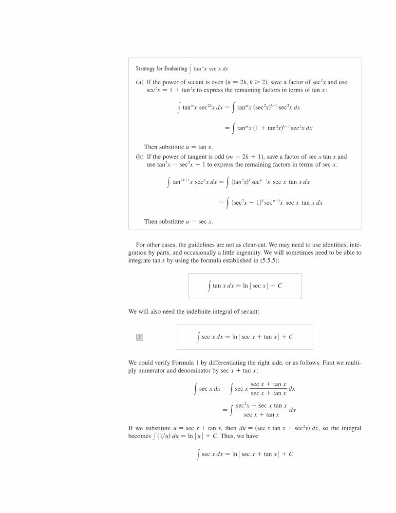
Strategy for Evaluating
(a) If the power of secant is even , save a factor of and useto express the remaining factors in terms of :
Then substitute .
(b) If the power of tangent is odd , save a factor of anduse to express the remaining factors in terms of :
Then substitute .
For other cases, the guidelines are not as clear-cut. We may need to use identities, inte-gration by parts, and occasionally a little ingenuity. We will sometimes need to be able tointegrate by using the formula established in (5.5.5):
We will also need the indefinite integral of secant:
We could verify Formula 1 by differentiating the right side, or as follows. First we multi-ply numerator and denominator by :
If we substitute , then , so the integralbecomes . Thus, we have
y sec x dx � ln sec x � tan x � C
x �1�u� du � ln u � Cdu � �sec x tan x � sec2x� dxu � sec x � tan x
� y sec2x � sec x tan x
sec x � tan x dx
y sec x dx � y sec x sec x � tan x
sec x � tan x dx
sec x � tan x
y sec x dx � ln sec x � tan x � C1
y tan x dx � ln sec x � C
tan x
u � sec x
� y �sec2x � 1�k secn�1x sec x tan x dx
y tan2k�1x secnx dx � y �tan2x�k secn�1x sec x tan x dx
sec xtan2x � sec2x � 1sec x tan x�m � 2k � 1�
u � tan x
� y tanmx �1 � tan2x�k�1 sec2x dx
y tanmx sec2kx dx � y tanmx �sec2x�k�1 sec2x dx
tan xsec2x � 1 � tan2xsec2x�n � 2k, k � 2�
y tanmx secnx dx
486 ❙ ❙ ❙ ❙ CHAPTER 7 TECHNIQUES OF INTEGRATION

EXAMPLE 7 Find .
SOLUTION Here only occurs, so we use to rewrite a factor interms of :
In the first integral we mentally substituted so that .
If an even power of tangent appears with an odd power of secant, it is helpful to expressthe integrand completely in terms of . Powers of may require integration byparts, as shown in the following example.
EXAMPLE 8 Find .
SOLUTION Here we integrate by parts with
Then
Using Formula 1 and solving for the required integral, we get
Integrals such as the one in the preceding example may seem very special but theyoccur frequently in applications of integration, as we will see in Chapter 8. Integrals of the form can be found by similar methods because of the identity
.Finally, we can make use of another set of trigonometric identities:
To evaluate the integrals (a) , (b) , or(c) , use the corresponding identity:
(a)
(b)
(c) cos A cos B � 12 �cos�A � B� � cos�A � B��
sin A sin B � 12 �cos�A � B� � cos�A � B��
sin A cos B � 12 �sin�A � B� � sin�A � B��
x cos mx cos nx dxx sin mx sin nx dxx sin mx cos nx dx2
1 � cot2x � csc2xx cotmx cscnx dx
y sec3x dx � 12 (sec x tan x � ln sec x � tan x ) � C
� sec x tan x � y sec3x dx � y sec x dx
� sec x tan x � y sec x �sec2x � 1� dx
y sec3x dx � sec x tan x � y sec x tan2x dx
du � sec x tan x dx v � tan x
u � sec x dv � sec2x dx
y sec3x dx
sec xsec x
du � sec2x dxu � tan x
�tan2x
2� ln sec x � C
� y tan x sec2x dx � y tan x dx
� y tan x �sec2x � 1� dx
y tan3x dx � y tan x tan2x dx
sec2xtan2xtan2x � sec2x � 1tan x
y tan3x dx
SECTION 7.2 TRIGONOMETRIC INTEGRALS ❙ ❙ ❙ ❙ 487
|||| These product identities are discussed inAppendix D.

31. 32.
33. 34.
35. 36.
37. 38.
39. 40.
42.
43. 44.
45. 46.
47.
48. If , express the value of
in terms of .
; 49–52 |||| Evaluate the indefinite integral. Illustrate, and check thatyour answer is reasonable, by graphing both the integrand and itsantiderivative (taking .
49. 50.
51. 52.
Find the average value of the function onthe interval .���, ��
f �x� � sin2x cos3x53.
■■ ■■ ■■ ■■ ■■ ■■ ■■ ■■ ■■ ■■ ■■ ■■
y sec4 x
2 dxy sin 3x sin 6x dx
y sin4x cos4x dxy sin5x dx
C � 0�
Ix��40 tan8x sec x dx
x��40 tan6x sec x dx � I
■■ ■■ ■■ ■■ ■■ ■■ ■■ ■■ ■■ ■■ ■■ ■■
y t sec2�t 2� tan4�t 2� dt
y dx
cos x � 1y 1 � tan2x
sec2x dx
y cos x � sin x
sin 2x dxy cos 7� cos 5� d�
y sin 3x cos x dxy sin 5x sin 2x dx41.
y��3
��6 csc3x dxy csc x dx
y csc 4x cot 6x dxy cot 3� csc3� d�
y��2
��4 cot3x dxy
��2
��6 cot2x dx
y tan2x sec x dxy tan3�
cos4� d�
y tan6�ay� dyy tan5x dx1–47 |||| Evaluate the integral.
1. 2.
4.
5. 6.
8.
9. 10.
11. 12.
13.
15. 16.
17. 18.
19. 20.
21. 22.
24.
25. 26.
27. 28.
30. y��3
0 tan5x sec6x dxy tan3x sec x dx29.
y tan3�2x� sec5�2x� dxy��3
0 tan5x sec4x dx
y��4
0 sec4� tan4� d�y sec6t dt
y tan4x dxy tan2x dx23.
y��2
0 sec4�t�2� dty sec2x tan x dx
y cos2x sin 2x dxy 1 � sin x
cos x dx
y cot5� sin4� d�y cos2x tan3x dx
y cos � cos5�sin �� d�y sin3x scos x dx
y��2
0 sin2x cos2x dx14.y
��4
0 sin4x cos2x dx
y x cos2x dxy �1 � cos ��2 d�
y�
0 cos6� d�y
�
0 sin4�3t� dt
y��2
0 sin2�2�� d�y
��2
0 cos2� d�7.
y sin3�mx� dxy cos5x sin4x dx
y��2
0 cos5x dxy
3��4
��2 sin5x cos3x dx3.
y sin6x cos3x dxy sin3x cos2x dx
|||| 7.2 Exercises
488 ❙ ❙ ❙ ❙ CHAPTER 7 TECHNIQUES OF INTEGRATION
EXAMPLE 9 Evaluate .
SOLUTION This integral could be evaluated using integration by parts, but it’s easier to usethe identity in Equation 2(a) as follows:
� 12 (cos x �
19 cos 9x� � C
� 12 y ��sin x � sin 9x� dx
y sin 4x cos 5x dx � y 12 �sin��x� � sin 9x� dx
y sin 4x cos 5x dx

SECTION 7.3 TRIGONOMETRIC SUBSTITUTION ❙ ❙ ❙ ❙ 489
64. Household electricity is supplied in the form of alternating current that varies from V to V with a frequency of 60 cycles per second (Hz). The voltage is thus given by the equation
where is the time in seconds. Voltmeters read the RMS (root-mean-square) voltage, which is the square root of the averagevalue of over one cycle.(a) Calculate the RMS voltage of household current.(b) Many electric stoves require an RMS voltage of 220 V.
Find the corresponding amplitude needed for the voltage.
65–67 |||| Prove the formula, where and are positive integers.
65.
66.
67.
68. A finite Fourier series is given by the sum
Show that the th coefficient is given by the formula
am �1
� y
�
�� f �x� sin mx dx
amm
� a1 sin x � a2 sin 2x � � � � � aN sin Nx
f �x� � N
n�1 an sin nx
■■ ■■ ■■ ■■ ■■ ■■ ■■ ■■ ■■ ■■ ■■ ■■
y�
�� cos mx cos nx dx � �0
�
if m � n
if m � n
y�
�� sin mx sin nx dx � �0
�
if m � n
if m � n
y�
�� sin mx cos nx dx � 0
nm
E�t� � A sin�120�t�A
�E�t��2
t
E�t� � 155 sin�120� t�
�15515554. Evaluate by four methods: (a) the substitution
, (b) the substitution , (c) the identity, and (d) integration by parts. Explain the
different appearances of the answers.
55–56 |||| Find the area of the region bounded by the given curves.
55.
56.
; 57–58 |||| Use a graph of the integrand to guess the value of theintegral. Then use the methods of this section to prove that yourguess is correct.
57. 58.
59–62 |||| Find the volume obtained by rotating the region boundedby the given curves about the specified axis.
, , , ; about the -axis
60. , , , ; about the -axis
61. , , , ; about
62. , , , ; about
63. A particle moves on a straight line with velocity function. Find its position function if
f �0� � 0.s � f �t�v�t� � sin t cos2t
■■ ■■ ■■ ■■ ■■ ■■ ■■ ■■ ■■ ■■ ■■ ■■
y � 1x � ��2x � 0y � 0y � cos x
y � �1x � ��2x � 0y � 0y � cos x
xx � ��4x � 0y � 0y � tan2x
xy � 0x � �x � ��2y � sin x59.
■■ ■■ ■■ ■■ ■■ ■■ ■■ ■■ ■■ ■■ ■■ ■■
y2
0 sin 2�x cos 5�x dxy
2�
0 cos3x dx
■■ ■■ ■■ ■■ ■■ ■■ ■■ ■■ ■■ ■■ ■■ ■■
x � ��2x � 0, y � 2 sin2x,y � sin x,
x � ��2x � 0, y � sin3x,y � sin x,
sin 2x � 2 sin x cos xu � sin xu � cos x
x sin x cos x dx
|||| 7.3 T r i g o n o m e t r i c S u b s t i t u t i o n
In finding the area of a circle or an ellipse, an integral of the form arises,where . If it were , the substitution would be effective
but, as it stands, is more difficult. If we change the variable from to bythe substitution , then the identity allows us to get rid of theroot sign because
Notice the difference between the substitution (in which the new variable isa function of the old one) and the substitution (the old variable is a function ofthe new one).
In general we can make a substitution of the form by using the SubstitutionRule in reverse. To make our calculations simpler, we assume that has an inverse func-tion; that is, is one-to-one. In this case, if we replace by and by in the SubstitutionRule (Equation 5.5.4), we obtain
This kind of substitution is called inverse substitution.
y f �x� dx � y f �t�t��t�t� dt
txxut
t
x � t�t�
x � a sin �u � a 2 � x 2
sa 2 � x 2 � sa 2 � a 2 sin2� � sa 2�1 � sin2�� � sa 2 cos2� � a cos �
1 � sin2� � cos2�x � a sin ��xx sa 2 � x 2 dx
u � a 2 � x 2x xsa 2 � x 2 dxa � 0
x sa 2 � x 2 dx

490 ❙ ❙ ❙ ❙ CHAPTER 7 TECHNIQUES OF INTEGRATION
We can make the inverse substitution provided that it defines a one-to-onefunction. This can be accomplished by restricting to lie in the interval .
In the following table we list trigonometric substitutions that are effective for the givenradical expressions because of the specified trigonometric identities. In each case the restric-tion on is imposed to ensure that the function that defines the substitution is one-to-one.(These are the same intervals used in Appendix D in defining the inverse functions.)
Table of Trigonometric Substitutions
EXAMPLE 1 Evaluate .
SOLUTION Let , where . Then and
(Note that because .) Thus, the Inverse Substitution Rulegives
Since this is an indefinite integral, we must return to the original variable . This can bedone either by using trigonometric identities to express in terms of or by drawing a diagram, as in Figure 1, where is interpreted as an angle of a right triangle.Since , we label the opposite side and the hypotenuse as having lengths and .Then the Pythagorean Theorem gives the length of the adjacent side as , so wecan simply read the value of from the figure:
(Although in the diagram, this expression for is valid even when .)Since , we have and so
y s9 � x 2
x 2 dx � �
s9 � x 2
x� sin�1� x
3� � C
� � sin�1�x�3�sin � � x�3� � 0cot �� � 0
cot � �s9 � x 2
x
cot �s9 � x 2
3xsin � � x�3�
sin � � x�3cot �x
� �cot � � � � C
� y �csc2� � 1� d�
� y cos2�
sin2� d� � y cot2� d�
y s9 � x 2
x 2 dx � y 3 cos �
9 sin2� 3 cos � d�
���2 � ��2cos � � 0
s9 � x 2 � s9 � 9 sin2� � s9 cos2� � 3 cos � � 3 cos �
dx � 3 cos � d����2 � ��2x � 3 sin �
y s9 � x 2
x 2 dx
�
����2, ��2��x � a sin �
3
¨
x
œ„„„„„9-≈
FIGURE 1
sin ¨= x3
Expression Substitution Identity
sec2� � 1 � tan2�x � a sec �, 0 � ��
2or � � �
3�
2sx 2 � a 2
1 � tan2� � sec2�x � a tan �, ��
2� � �
�
2sa 2 � x 2
1 � sin2� � cos2�x � a sin �, ��
2 �
�
2sa 2 � x 2

SECTION 7.3 TRIGONOMETRIC SUBSTITUTION ❙ ❙ ❙ ❙ 491
EXAMPLE 2 Find the area enclosed by the ellipse
SOLUTION Solving the equation of the ellipse for , we get
Because the ellipse is symmetric with respect to both axes, the total area is four timesthe area in the first quadrant (see Figure 2). The part of the ellipse in the first quadrant isgiven by the function
and so
To evaluate this integral we substitute . Then . To change thelimits of integration we note that when , , so ; when ,
, so . Also
since . Therefore
We have shown that the area of an ellipse with semiaxes and is . In particular,taking , we have proved the famous formula that the area of a circle withradius is .
NOTE ■■ Since the integral in Example 2 was a definite integral, we changed the limits ofintegration and did not have to convert back to the original variable .
EXAMPLE 3 Find .
SOLUTION Let . Then and
Thus, we have
y dx
x 2sx 2 � 4
� y 2 sec2� d�
4 tan2� � 2 sec ��
1
4 y
sec �
tan2� d�
sx 2 � 4 � s4�tan 2� � 1� � s4 sec2� � 2 sec � � 2 sec �
dx � 2 sec2� d�x � 2 tan �, ���2 � � � ��2
y 1
x 2sx 2 � 4
dx
x
�r 2ra � b � r
�abba
� �ab
� 2ab[� �12 sin 2�]0
��2� 2ab��
2� 0 � 0�
� 4ab y��2
0 cos2� d� � 4ab y
��2
0 12 �1 � cos 2�� d�
A � 4 b
a y
a
0 sa 2 � x 2 dx � 4
b
a y
��2
0 a cos � � a cos � d�
0 � ��2
sa 2 � x 2 � sa 2 � a 2 sin2� � sa 2 cos2� � a cos � � a cos �
� � ��2sin � � 1x � a� � 0sin � � 0x � 0
dx � a cos � d�x � a sin �
14 A � y
a
0 b
a sa 2 � x 2 dx
0 x ay �b
a sa 2 � x 2
A
y � �b
a sa 2 � x 2or
y 2
b 2 � 1 �x 2
a 2 �a 2 � x 2
a 2
y
x 2
a 2 � y 2
b 2 � 1
FIGURE 2
≈a@
¥b@
+ =1
y
0 x
(0, b)
(a, 0)

492 ❙ ❙ ❙ ❙ CHAPTER 7 TECHNIQUES OF INTEGRATION
To evaluate this trigonometric integral we put everything in terms of and :
Therefore, making the substitution , we have
We use Figure 3 to determine that and so
EXAMPLE 4 Find .
SOLUTION It would be possible to use the trigonometric substitution here (as inExample 3). But the direct substitution is simpler, because then and
NOTE ■■ Example 4 illustrates the fact that even when trigonometric substitutions are pos-sible, they may not give the easiest solution. You should look for a simpler method first.
EXAMPLE 5 Evaluate , where .
SOLUTION 1 We let , where or . Thenand
Therefore
The triangle in Figure 4 gives , so we have
� ln x � sx 2 � a 2 � ln a � C
y dx
sx 2 � a 2� ln � x
a�
sx 2 � a 2
a � � C
tan � � sx 2 � a 2�a
� y sec � d� � ln sec � � tan � � C
y dx
sx 2 � a 2� y
a sec � tan �
a tan � d�
sx 2 � a 2 � sa 2�sec2� � 1� � sa 2 tan2� � a tan � � a tan �
dx � a sec � tan � d�� � � � 3��20 � � � ��2x � a sec �
a � 0y dx
sx 2 � a 2
y x
sx 2 � 4 dx �
1
2 y
du
su� su � C � sx 2 � 4 � C
du � 2x dxu � x 2 � 4x � 2 tan �
y x
sx 2 � 4 dx
y dx
x 2sx 2 � 4
� �sx 2 � 4
4x� C
csc � � sx 2 � 4�x
� �csc �
4� C
�1
4 ��
1
u� � C � �1
4 sin �� C
y dx
x 2sx 2 � 4
�1
4 y
cos �
sin2� d� �
1
4 y
du
u 2
u � sin �
sec�
tan2��
1
cos ��
cos2�
sin2��
cos �
sin2�
cos �sin �
œ„„„„„≈+4
2
¨
x
FIGUR E 3
tan ¨= x2
FIGU RE 4
sec ¨= xa
œ„„„„„
a¨
x≈-a@
SECTION 7.3 TRIGONOMETRIC SUBSTITUTION ❙ ❙ ❙ ❙ 493
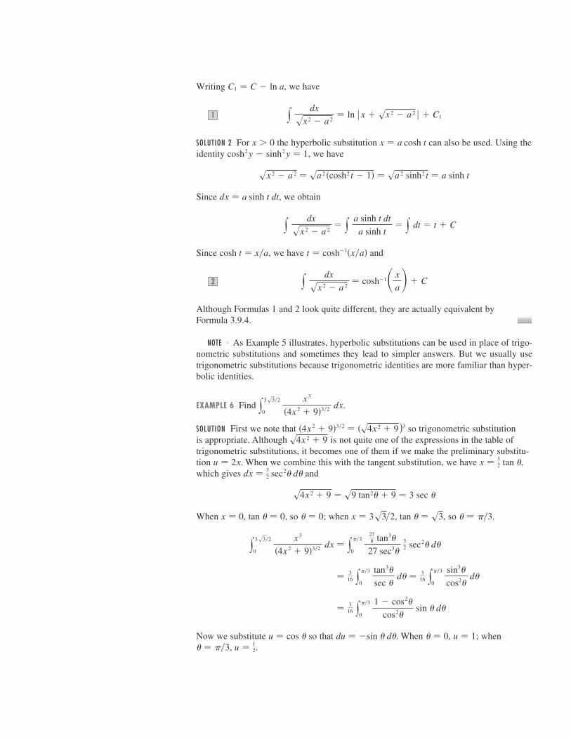
Writing , we have
SOLUTION 2 For the hyperbolic substitution can also be used. Using theidentity , we have
Since , we obtain
Since , we have and
Although Formulas 1 and 2 look quite different, they are actually equivalent byFormula 3.9.4.
NOTE ■■ As Example 5 illustrates, hyperbolic substitutions can be used in place of trigo-nometric substitutions and sometimes they lead to simpler answers. But we usually usetrigonometric substitutions because trigonometric identities are more familiar than hyper-bolic identities.
EXAMPLE 6 Find .
SOLUTION First we note that so trigonometric substitution is appropriate. Although is not quite one of the expressions in the table oftrigonometric substitutions, it becomes one of them if we make the preliminary substitu-tion . When we combine this with the tangent substitution, we have ,which gives and
When , , so ; when , , so .
Now we substitute so that . When , ; when.� � ��3, u � 1
2
u � 1� � 0du � �sin � d�u � cos �
� 316 y
��3
0 1 � cos2�
cos2� sin � d�
� 316 y
��3
0 tan3�
sec � d� � 3
16 y��3
0 sin3�
cos2� d�
y3 s3�2
0
x 3
�4x 2 � 9�3�2 dx � y��3
0
278 tan3�
27 sec3� 32 sec2� d�
� � ��3tan � � s3x � 3s3�2� � 0tan � � 0x � 0
s4x 2 � 9 � s9 tan2� � 9 � 3 sec �
dx � 32 sec2� d�
x � 32 tan �u � 2x
s4x 2 � 9�4x 2 � 9�3�2 � �s4x 2 � 9)3
y3 s3�2
0
x 3
�4x 2 � 9�3�2 dx
y dx
sx 2 � a 2� cosh�1� x
a� � C2
t � cosh�1�x�a�cosh t � x�a
y dx
sx 2 � a 2� y
a sinh t dt
a sinh t� y dt � t � C
dx � a sinh t dt
sx 2 � a 2 � sa 2 �cosh2 t � 1� � sa 2 sinh2 t � a sinh t
cosh2y � sinh2y � 1x � a cosh tx � 0
y dx
sx 2 � a 2� ln x � sx 2 � a 2 � C11
C1 � C � ln a
4–30 |||| Evaluate the integral.
4.
5. 6.
8.
9. 10. y t 5
st 2 � 2 dty
dx
sx 2 � 16
y sx 2 � a 2
x 4 dxy
1
x 2s25 � x 2
dx7.
y2
0 x 3
sx 2 � 4 dxy2
s2
1
t 3st 2 � 1
dt
y2 s3
0
x 3
s16 � x 2 dx
1–3 |||| Evaluate the integral using the indicated trigonometric substitution. Sketch and label the associated right triangle.
1. ;
2. ;
;
■■ ■■ ■■ ■■ ■■ ■■ ■■ ■■ ■■ ■■ ■■ ■■
x � 3 tan �y x 3
sx 2 � 9 dx3.
x � 3 sin �y x 3s9 � x 2 dx
x � 3 sec �y 1
x 2sx 2 � 9
dx
|||| 7.3 Exercises
494 ❙ ❙ ❙ ❙ CHAPTER 7 TECHNIQUES OF INTEGRATION
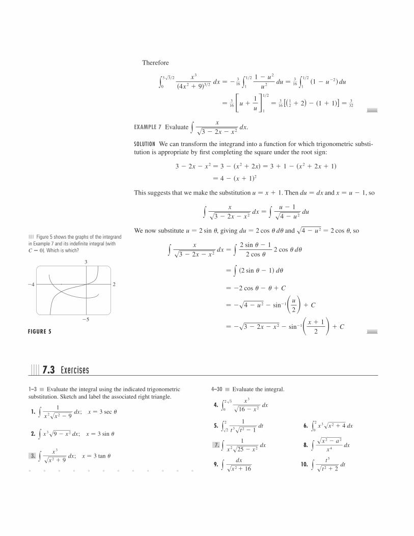
Therefore
EXAMPLE 7 Evaluate .
SOLUTION We can transform the integrand into a function for which trigonometric substi-tution is appropriate by first completing the square under the root sign:
This suggests that we make the substitution . Then and , so
We now substitute , giving and , so
� �s3 � 2x � x 2 � sin�1� x � 1
2 � � C
� �s4 � u 2 � sin�1�u
2� � C
� �2 cos � � � � C
� y �2 sin � � 1� d�
y x
s3 � 2x � x 2 dx � y
2 sin � � 1
2 cos � 2 cos � d�
s4 � u 2 � 2 cos �du � 2 cos � d�u � 2 sin �
y x
s3 � 2x � x 2 dx � y
u � 1
s4 � u 2 du
x � u � 1du � dxu � x � 1
� 4 � �x � 1�2
3 � 2x � x 2 � 3 � �x 2 � 2x� � 3 � 1 � �x 2 � 2x � 1�
y x
s3 � 2x � x 2 dx
� 316 �u �
1
u�1
1�2
� 316 [( 1
2 � 2) � �1 � 1�] � 332
y3 s3�2
0
x 3
�4x 2 � 9�3�2 dx � �316 y
1�2
1 1 � u 2
u 2 du � 316 y
1�2
1 �1 � u�2 � du
|||| Figure 5 shows the graphs of the integrandin Example 7 and its indefinite integral (with
). Which is which?C � 0
_4
_5
3
2
FIGURE 5

SECTION 7.3 TRIGONOMETRIC SUBSTITUTION ❙ ❙ ❙ ❙ 495
equation . Then is the sum of the area of the triangle and the area of the region in the figure.]
; 36. Evaluate the integral
Graph the integrand and its indefinite integral on the samescreen and check that your answer is reasonable.
; 37. Use a graph to approximate the roots of the equation. Then approximate the area bounded by
the curve and the line .
38. A charged rod of length produces an electric field at pointgiven by
where is the charge density per unit length on the rod and is the free space permittivity (see the figure). Evaluate the inte-gral to determine an expression for the electric field .
39. Find the area of the crescent-shaped region (called a lune)bounded by arcs of circles with radii and . (See the figure.)
40. A water storage tank has the shape of a cylinder with diameter10 ft. It is mounted so that the circular cross-sections are verti-cal. If the depth of the water is 7 ft, what percentage of thetotal capacity is being used?
41. A torus is generated by rotating the circle about the -axis. Find the volume enclosed by the torus.x
x 2 � �y � R�2 � r 2
R
r
Rr
0 x
y
L
P (a, b)
E�P�
�0�
E�P� � yL�a
�a
�b
4��0�x 2 � b 2 �3�2 dx
P�a, b�L
y � 2 � xy � x 2s4 � x 2
x 2s4 � x 2 � 2 � x
y dx
x 4sx 2 � 2
O x
y
RQ¨
P
PQRPOQAx 2 � y 2 � r 2
11. 12.
14.
15. 16.
18.
19. 20.
21.
23. 24.
25. 26.
27. 28.
29. 30.
(a) Use trigonometric substitution to show that
(b) Use the hyperbolic substitution to show that
These formulas are connected by Formula 3.9.3.
32. Evaluate
(a) by trigonometric substitution.(b) by the hyperbolic substitution .
33. Find the average value of , .
34. Find the area of the region bounded by the hyperbolaand the line .
35. Prove the formula for the area of a sector of a circlewith radius and central angle . [Hint: Assume and place the center of the circle at the origin so it has the
0 � � � ��2�rA � 1
2 r 2�
x � 39x 2 � 4y 2 � 36
1 x 7f �x� � sx 2 � 1�x
x � a sinh t
y x 2
�x 2 � a 2 �3�2 dx
y dx
sx 2 � a 2� sinh�1� x
a� � C
x � a sinh t
y dx
sx 2 � a 2� ln(x � sx 2 � a 2 ) � C
31.
■■ ■■ ■■ ■■ ■■ ■■ ■■ ■■ ■■ ■■ ■■ ■■
y��2
0
cos t
s1 � sin2t dty xs1 � x 4 dx
y dx
�5 � 4x � x 2 �5�2y dx
�x 2 � 2x � 2�2
y x 2
s4x � x 2 dxy
1
s9x 2 � 6x � 8 dx
y dt
st 2 � 6t � 13y s5 � 4x � x 2 dx
y1
0 sx 2 � 1 dx22.y
2�3
0 x 3
s4 � 9x 2 dx
y t
s25 � t 2 dty
s1 � x 2
x dx
y dx
�ax�2 � b 2 3�2y x
sx 2 � 7 dx17.
y dx
x 2s16x 2 � 9y
x 2
�a 2 � x 2 �3�2 dx
y du
us5 � u 2y sx 2 � 9
x 3 dx13.
y1
0 xsx 2 � 4 dxy s1 � 4x 2 dx

496 ❙ ❙ ❙ ❙ CHAPTER 7 TECHNIQUES OF INTEGRATION
|||| 7.4 I n t e g r a t i o n o f R a t i o n a l F u n c t i o n s b y P a r t i a l F r a c t i o n s
In this section we show how to integrate any rational function (a ratio of polynomials) byexpressing it as a sum of simpler fractions, called partial fractions, that we already knowhow to integrate. To illustrate the method, observe that by taking the fractions and to a common denominator we obtain
If we now reverse the procedure, we see how to integrate the function on the right side ofthis equation:
To see how the method of partial fractions works in general, let’s consider a rationalfunction
where and are polynomials. It’s possible to express as a sum of simpler fractionsprovided that the degree of is less than the degree of . Such a rational function is calledproper. Recall that if
where , then the degree of is and we write .If is improper, that is, , then we must take the preliminary step
of dividing into (by long division) until a remainder is obtained such that. The division statement is
where and are also polynomials.As the following example illustrates, sometimes this preliminary step is all that is
required.
EXAMPLE 1 Find .
SOLUTION Since the degree of the numerator is greater than the degree of the denominator,we first perform the long division. This enables us to write
�x 3
3�
x 2
2� 2x � 2 ln � x � 1 � � C
y x 3 � x
x � 1 dx � y �x 2 � x � 2 �
2
x � 1� dx
y x 3 � x
x � 1 dx
RS
f �x� �P�x�Q�x�
� S�x� �R�x�Q�x�
1
deg�R� � deg�Q�R�x�PQ
deg�P� deg�Q�fdeg�P� � nnPan � 0
P�x� � anxn � an�1xn�1 � � � � � a1x � a0
QPfQP
f �x� �P�x�Q�x�
� 2 ln � x � 1 � � ln � x � 2 � � C
y x � 5
x 2 � x � 2 dx � y � 2
x � 1�
1
x � 2� dx
2
x � 1�
1
x � 2�
2�x � 2� � �x � 1��x � 1��x � 2�
�x � 5
x 2 � x � 2
1��x � 2�2��x � 1�
x-1≈+x +2
˛-≈≈+x≈-x
2x2x-2
2
˛ +x)

SECTION 7.4 INTEGRATION OF RATIONAL FUNCTIONS BY PARTIAL FRACTIONS ❙ ❙ ❙ ❙ 497
The next step is to factor the denominator as far as possible. It can be shown thatany polynomial can be factored as a product of linear factors (of the form ) andirreducible quadratic factors (of the form , where ). For in-stance, if , we could factor it as
The third step is to express the proper rational function (from Equation 1) asa sum of partial fractions of the form
A theorem in algebra guarantees that it is always possible to do this. We explain the detailsfor the four cases that occur.
CASE I ■■ The denominator is a product of distinct linear factors.This means that we can write
where no factor is repeated (and no factor is a constant multiple of another). In this casethe partial fraction theorem states that there exist constants such that
These constants can be determined as in the following example.
EXAMPLE 2 Evaluate .
SOLUTION Since the degree of the numerator is less than the degree of the denominator,we don’t need to divide. We factor the denominator as
Since the denominator has three distinct linear factors, the partial fraction decompositionof the integrand (2) has the form
To determine the values of , , and , we multiply both sides of this equation by theproduct of the denominators, , obtaining
Expanding the right side of Equation 4 and writing it in the standard form for polyno-mials, we get
x 2 � 2x � 1 � �2A � B � 2C �x 2 � �3A � 2B � C �x � 2A5
x 2 � 2x � 1 � A�2x � 1��x � 2� � Bx�x � 2� � Cx�2x � 1�4
x �2x � 1��x � 2�CBA
x 2 � 2x � 1
x�2x � 1��x � 2��
A
x�
B
2x � 1�
C
x � 23
2x 3 � 3x 2 � 2x � x�2x 2 � 3x � 2� � x �2x � 1��x � 2�
y x 2 � 2x � 1
2x 3 � 3x 2 � 2x dx
R�x�Q�x�
�A1
a1x � b1�
A2
a2x � b2� � � � �
Ak
akx � bk2
A1, A2, . . . , Ak
Q�x� � �a1x � b1 ��a2x � b2 � � � � �ak x � bk�
Q�x�
Ax � B
�ax 2 � bx � c� jorA
�ax � b�i
R�x��Q�x�
Q�x� � �x 2 � 4��x 2 � 4� � �x � 2��x � 2��x 2 � 4�
Q�x� � x 4 � 16b 2 � 4ac � 0ax 2 � bx � c
ax � bQQ�x�
|||| Another method for finding , , and is given in the note after this example.
CBA

498 ❙ ❙ ❙ ❙ CHAPTER 7 TECHNIQUES OF INTEGRATION
The polynomials in Equation 5 are identical, so their coefficients must be equal. Thecoefficient of on the right side, , must equal the coefficient of on theleft side—namely, 1. Likewise, the coefficients of are equal and the constant terms areequal. This gives the following system of equations for , , and :
Solving, we get , , and , and so
In integrating the middle term we have made the mental substitution , whichgives and .
NOTE ■■ We can use an alternative method to find the coefficients , , and in Example 2. Equation 4 is an identity; it is true for every value of . Let’s choose values of
that simplify the equation. If we put in Equation 4, then the second and third termson the right side vanish and the equation then becomes , or . Likewise,
gives and gives , so and . (You may objectthat Equation 3 is not valid for , , or , so why should Equation 4 be valid for thosevalues? In fact, Equation 4 is true for all values of , even , , and . See Exercise 67for the reason.)
EXAMPLE 3 Find , where .
SOLUTION The method of partial fractions gives
and therefore
Using the method of the preceding note, we put in this equation and get, so . If we put , we get , so .
Thus
�1
2a (ln � x � a � � ln � x � a �) � C
y dx
x 2 � a 2 �1
2a y � 1
x � a�
1
x � a� dx
B � �1��2a�B��2a� � 1x � �aA � 1��2a�A�2a� � 1x � a
A�x � a� � B�x � a� � 1
1
x 2 � a 2 �1
�x � a��x � a��
A
x � a�
B
x � a
a � 0y dx
x 2 � a 2
�212x � 0x
�212x � 0
C � �1
10B � 1510C � �1x � �25B�4 � 1
4x � 12
A � 12�2A � �1
x � 0xx
CBA
dx � du�2du � 2 dxu � 2x � 1
� 12 ln � x � �
110 ln � 2x � 1 � �
110 ln � x � 2 � � K
y x 2 � 2x � 1
2x 3 � 3x 2 � 2x dx � y �1
2 1
x�
1
5
1
2x � 1�
1
10
1
x � 2� dx
C � �110B � 1
5A � 12
�2A � 2B � 2C � �1
3A � 2B � C � 2
2A � B � 2C � 1
CBAx
x 22A � B � 2Cx 2|||| Figure 1 shows the graphs of the integrandin Example 2 and its indefinite integral (with
). Which is which?K � 0
FIGURE 1
_3
_2
2
3
|||| We could check our work by taking the termsto a common denominator and adding them.
SECTION 7.4 INTEGRATION OF RATIONAL FUNCTIONS BY PARTIAL FRACTIONS ❙ ❙ ❙ ❙ 499
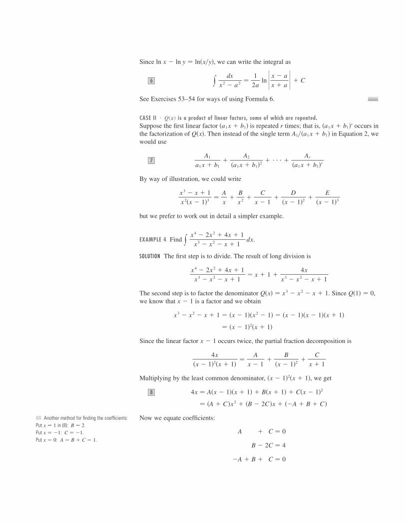
Since , we can write the integral as
See Exercises 53–54 for ways of using Formula 6.
CASE II ■■ is a product of linear factors, some of which are repeated.Suppose the first linear factor is repeated times; that is, occurs inthe factorization of . Then instead of the single term in Equation 2, wewould use
By way of illustration, we could write
but we prefer to work out in detail a simpler example.
EXAMPLE 4 Find .
SOLUTION The first step is to divide. The result of long division is
The second step is to factor the denominator . Since ,we know that is a factor and we obtain
Since the linear factor occurs twice, the partial fraction decomposition is
Multiplying by the least common denominator, , we get
Now we equate coefficients:
�A � B � C � 0
A � B � 2C � 4
A � B � C � 0
� �A � C �x 2 � �B � 2C �x � ��A � B � C �
4x � A�x � 1��x � 1� � B�x � 1� � C�x � 1�28
�x � 1�2�x � 1�
4x
�x � 1�2�x � 1��
A
x � 1�
B
�x � 1�2 �C
x � 1
x � 1
� �x � 1�2�x � 1�
x 3 � x 2 � x � 1 � �x � 1��x 2 � 1� � �x � 1��x � 1��x � 1�
x � 1Q�1� � 0Q�x� � x 3 � x 2 � x � 1
x 4 � 2x 2 � 4x � 1
x 3 � x 2 � x � 1� x � 1 �
4x
x 3 � x 2 � x � 1
y x 4 � 2x 2 � 4x � 1
x 3 � x 2 � x � 1 dx
x 3 � x � 1
x 2�x � 1�3 �A
x�
B
x 2 �C
x � 1�
D
�x � 1�2 �E
�x � 1�3
A1
a1x � b1�
A2
�a1x � b1�2 � � � � �Ar
�a1x � b1�r7
A1��a1 x � b1�Q�x��a1x � b1�rr�a1x � b1�
Q�x�
y dx
x 2 � a 2 �1
2a ln � x � a
x � a � � C6
ln x � ln y � ln�x�y�
|||| Another method for finding the coefficients:Put in (8): .Put : .Put : .A � B � C � 1x � 0
C � �1x � �1B � 2x � 1
500 ❙ ❙ ❙ ❙ CHAPTER 7 TECHNIQUES OF INTEGRATION
Solving, we obtain , , and , so
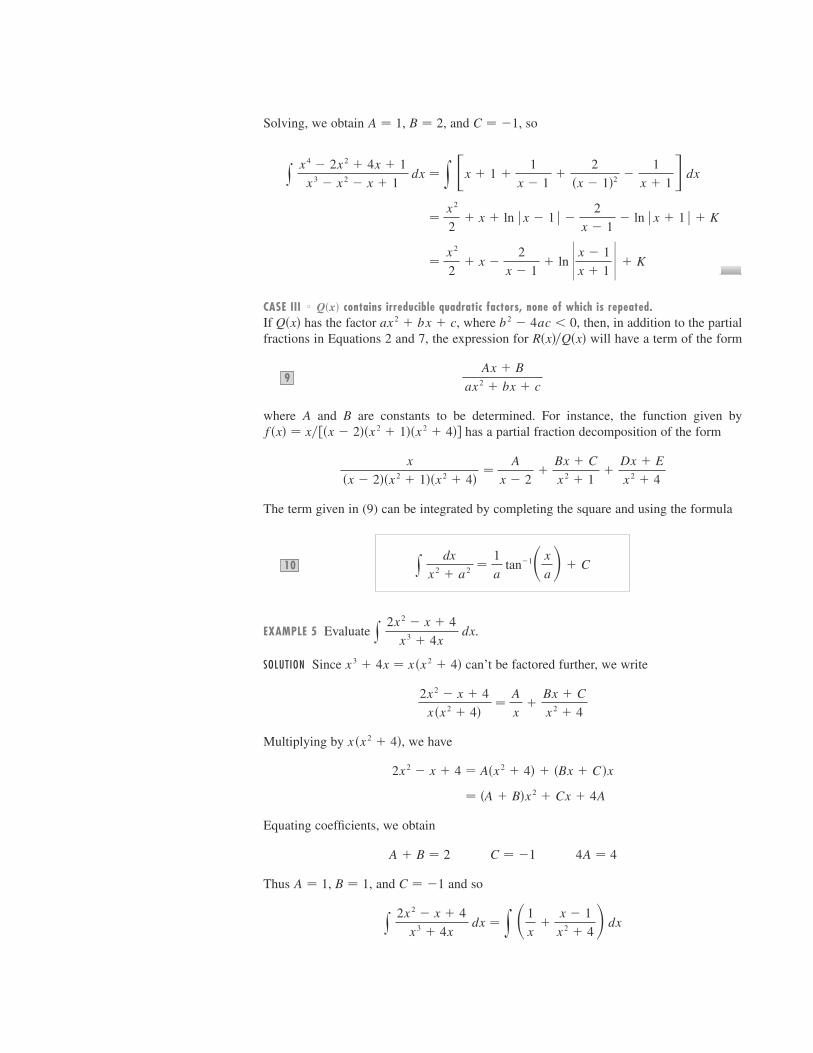
CASE III ■■ contains irreducible quadratic factors, none of which is repeated.If has the factor , where , then, in addition to the partialfractions in Equations 2 and 7, the expression for will have a term of the form
where and are constants to be determined. For instance, the function given byhas a partial fraction decomposition of the form
The term given in (9) can be integrated by completing the square and using the formula
EXAMPLE 5 Evaluate .
SOLUTION Since can’t be factored further, we write
Multiplying by , we have
Equating coefficients, we obtain
Thus , , and and so
y 2x 2 � x � 4
x 3 � 4x dx � y �1
x�
x � 1
x 2 � 4� dx
C � �1B � 1A � 1
4A � 4C � �1A � B � 2
� �A � B�x 2 � Cx � 4A
2x 2 � x � 4 � A�x 2 � 4� � �Bx � C �x
x�x 2 � 4�
2x 2 � x � 4
x �x 2 � 4��
A
x�
Bx � C
x 2 � 4
x 3 � 4x � x�x 2 � 4�
y 2x 2 � x � 4
x 3 � 4x dx
y dx
x 2 � a 2 �1
a tan�1� x
a� � C10
x
�x � 2��x 2 � 1��x 2 � 4��
A
x � 2�
Bx � C
x 2 � 1�
Dx � E
x 2 � 4
f �x� � x��x � 2��x 2 � 1��x 2 � 4�BA
Ax � B
ax 2 � bx � c9
R�x��Q�x�b 2 � 4ac � 0ax 2 � bx � cQ�x�
Q�x�
�x 2
2� x �
2
x � 1� ln � x � 1
x � 1 � � K
�x 2
2� x � ln � x � 1 � �
2
x � 1� ln � x � 1 � � K
y x 4 � 2x 2 � 4x � 1
x 3 � x 2 � x � 1 dx � y �x � 1 �
1
x � 1�
2
�x � 1�2 �1
x � 1� dx
C � �1B � 2A � 1

SECTION 7.4 INTEGRATION OF RATIONAL FUNCTIONS BY PARTIAL FRACTIONS ❙ ❙ ❙ ❙ 501
In order to integrate the second term we split it into two parts:
We make the substitution in the first of these integrals so that .We evaluate the second integral by means of Formula 10 with :
EXAMPLE 6 Evaluate .
SOLUTION Since the degree of the numerator is not less than the degree of the denomina-tor, we first divide and obtain
Notice that the quadratic is irreducible because its discriminant is. This means it can’t be factored, so we don’t need to use the
partial fraction technique.To integrate the given function we complete the square in the denominator:
This suggests that we make the substitution . Then, and, so
NOTE ■■ Example 6 illustrates the general procedure for integrating a partial fraction ofthe form
where b 2 � 4ac � 0Ax � B
ax 2 � bx � c
� x �18 ln�4x 2 � 4x � 3� �
1
4s2 tan�1�2x � 1
s2� � C
� x �18 ln�u 2 � 2� �
1
4�
1
s2 tan�1� u
s2� � C
� x �14 y
u
u 2 � 2 du �
14 y
1
u 2 � 2 du
� x �12 y
12 �u � 1� � 1
u 2 � 2 du � x �
14 y
u � 1
u 2 � 2 du
y 4x 2 � 3x � 2
4x 2 � 4x � 3 dx � y �1 �
x � 1
4x 2 � 4x � 3� dx
x � �u � 1��2du � 2 dxu � 2x � 1
4x 2 � 4x � 3 � �2x � 1�2 � 2
b 2 � 4ac � �32 � 04x 2 � 4x � 3
4x 2 � 3x � 2
4x 2 � 4x � 3� 1 �
x � 1
4x 2 � 4x � 3
y 4x 2 � 3x � 2
4x 2 � 4x � 3 dx
� ln � x � �12 ln�x 2 � 4� �
12 tan�1�x�2� � K
y 2x 2 � x � 4
x�x 2 � 4� dx � y
1
x dx � y
x
x 2 � 4 dx � y
1
x 2 � 4 dx
a � 2du � 2x dxu � x 2 � 4
y x � 1
x 2 � 4 dx � y
x
x 2 � 4 dx � y
1
x 2 � 4 dx

502 ❙ ❙ ❙ ❙ CHAPTER 7 TECHNIQUES OF INTEGRATION
We complete the square in the denominator and then make a substitution that brings theintegral into the form
Then the first integral is a logarithm and the second is expressed in terms of .
CASE IV ■■ contains a repeated irreducible quadratic factor.If has the factor , where , then instead of the singlepartial fraction (9), the sum
occurs in the partial fraction decomposition of . Each of the terms in (11) can beintegrated by first completing the square.
EXAMPLE 7 Write out the form of the partial fraction decomposition of the function
SOLUTION
EXAMPLE 8 Evaluate .
SOLUTION The form of the partial fraction decomposition is
Multiplying by , we have
If we equate coefficients, we get the system
which has the solution , , , , and . ThusE � 0D � 1C � �1B � �1A � 1
A � 1C � E � �12A � B � D � 2C � �1A � B � 0
� �A � B�x 4 � Cx 3 � �2A � B � D�x 2 � �C � E�x � A
� A�x 4 � 2x 2 � 1� � B�x 4 � x 2 � � C�x 3 � x� � Dx 2 � Ex
�x 3 � 2x 2 � x � 1 � A�x 2 � 1�2 � �Bx � C �x�x 2 � 1� � �Dx � E�x
x�x 2 � 1�2
1 � x � 2x 2 � x 3
x�x 2 � 1�2 �A
x�
Bx � C
x 2 � 1�
Dx � E
�x 2 � 1�2
y 1 � x � 2x 2 � x 3
x�x 2 � 1�2 dx
� A
x�
B
x � 1�
Cx � D
x 2 � x � 1�
Ex � F
x 2 � 1�
Gx � H
�x 2 � 1�2 �Ix � J
�x 2 � 1�3
x 3 � x 2 � 1
x�x � 1��x 2 � x � 1��x 2 � 1�3
x 3 � x 2 � 1
x�x � 1��x 2 � x � 1��x 2 � 1�3
R�x��Q�x�
A1x � B1
ax 2 � bx � c�
A2x � B2
�ax 2 � bx � c�2 � � � � �Ar x � Br
�ax 2 � bx � c�r11
b 2 � 4ac � 0�ax 2 � bx � c�rQ�x�Q�x�
tan�1
y Cu � D
u 2 � a 2 du � C y u
u 2 � a 2 du � D y 1
u 2 � a 2 du
|||| It would be extremely tedious to work out byhand the numerical values of the coefficients inExample 7. Most computer algebra systems,however, can find the numerical values veryquickly. For instance, the Maple command
or the Mathematica command
gives the following values:
I � �12 , J � 1
2
E � 158 , F � �
18 , G � H � 3
4 ,
A � �1, B � 18 , C � D � �1,
Apart[f]
convert�f, parfrac, x�
SECTION 7.4 INTEGRATION OF RATIONAL FUNCTIONS BY PARTIAL FRACTIONS ❙ ❙ ❙ ❙ 503
We note that sometimes partial fractions can be avoided when integrating a rational func-tion. For instance, although the integral
could be evaluated by the method of Case III, it’s much easier to observe that if, then and so
R a t i o n a l i z i n g S u b s t i t u t i o n s
Some nonrational functions can be changed into rational functions by means of appropri-ate substitutions. In particular, when an integrand contains an expression of the form
, then the substitution may be effective. Other instances appear in theexercises.
EXAMPLE 9 Evaluate .
SOLUTION Let . Then , so and . Therefore
We can evaluate this integral either by factoring as and usingpartial fractions or by using Formula 6 with :
� 2sx � 4 � 2 ln � sx � 4 � 2
sx � 4 � 2 � � C
� 2u � 8 �1
2 � 2 ln � u � 2
u � 2 � � C
y sx � 4
x dx � 2 y du � 8 y
du
u 2 � 4
a � 2�u � 2��u � 2�u 2 � 4
� 2 y �1 �4
u 2 � 4� du
y sx � 4
x dx � y
u
u 2 � 4 2u du � 2 y
u 2
u 2 � 4 du
dx � 2u dux � u 2 � 4u 2 � x � 4u � sx � 4
y sx � 4
x dx
u � sn
t�x�sn
t�x�
y x 2 � 1
x�x 2 � 3� dx � 1
3 ln � x 3 � 3x � � C
du � �3x 2 � 3� dxu � x�x 2 � 3� � x 3 � 3x
y x 2 � 1
x�x 2 � 3� dx
� ln � x � �12 ln�x 2 � 1� � tan�1x �
1
2�x 2 � 1�� K
� y dx
x� y
x
x 2 � 1 dx � y
dx
x 2 � 1� y
x dx
�x 2 � 1�2
y 1 � x � 2x 2 � x 3
x�x 2 � 1�2 dx � y �1
x�
x � 1
x 2 � 1�
x
�x 2 � 1�2� dx
|||| In the second and fourth terms we made themental substitution .u � x 2 � 1

32.
33. 34.
35. 36.
37. 38.
39–48 |||| Make a substitution to express the integrand as a rationalfunction and then evaluate the integral.
39. 40.
41. 42.
44.
45. [Hint: Substitute .]
46. [Hint: Substitute .]
48.
49–50 |||| Use integration by parts, together with the techniques ofthis section, to evaluate the integral.
49. 50.
; 51. Use a graph of to decide whetheris positive or negative. Use the graph to give a rough
estimate of the value of the integral and then use partialfractions to find the exact value.
; 52. Graph both and an antiderivative on thesame screen.
53–54 |||| Evaluate the integral by completing the square and usingFormula 6.
54.
55. The German mathematician Karl Weierstrass (1815–1897)noticed that the substitution will convert any t � tan�x�2�
■■ ■■ ■■ ■■ ■■ ■■ ■■ ■■ ■■ ■■ ■■ ■■
y 2x � 1
4x 2 � 12x � 7 dxy
dx
x 2 � 2x53.
y � 1��x 3 � 2x 2 �
x20 f �x� dx
f �x� � 1��x 2 � 2x � 3�
■■ ■■ ■■ ■■ ■■ ■■ ■■ ■■ ■■ ■■ ■■ ■■
y x tan�1x dxy ln�x 2 � x � 2� dx
■■ ■■ ■■ ■■ ■■ ■■ ■■ ■■ ■■ ■■ ■■ ■■
y cos x
sin2x � sin x dxy
e 2x
e 2x � 3e x � 2 dx47.
u � 12sxy
1
s3 x � s
4 x dx
u � 6sxy
1
sx � s3 x
dx
y3
1�3
sx
x 2 � x dxy
x 3
s3 x 2 � 1
dx43.
y1
0
1
1 � s3 x
dxy16
9
sx
x � 4 dx
y 1
x � sx � 2 dxy
1
xsx � 1 dx
■■ ■■ ■■ ■■ ■■ ■■ ■■ ■■ ■■ ■■ ■■ ■■
y x 4 � 1
x �x 2 � 1�2 dxy x � 3
�x 2 � 2x � 4�2 dx
y1
0
2x 3 � 5x
x 4 � 5x 2 � 4 dxy
dx
x 4 � x 2
y x 3
x 3 � 1 dxy
5
2
x 2 � 2x
x 3 � 3x 2 � 4 dx
y1
0
x
x 2 � 4x � 13 dxy
1
x 3 � 1 dx31.
1–6 |||| Write out the form of the partial fraction decomposition of the function (as in Example 7). Do not determine the numericalvalues of the coefficients.
1. (a) (b)
2. (a) (b)
3. (a) (b)
4. (a) (b)
(a) (b)
6. (a) (b)
7–38 |||| Evaluate the integral.
7. 8.
9. 10.
12.
13. 14.
15. 16.
18.
19. 20.
21. 22.
24.
26.
27. 28.
30. y x 3 � 2x 2 � x � 1
x 4 � 5x 2 � 4 dxy
x � 4
x 2 � 2x � 5 dx29.
y x 2 � 2x � 1
�x � 1�2�x 2 � 1� dxy
x 3 � x 2 � 2x � 1
�x 2 � 1��x 2 � 2� dx
y x 2 � x � 6
x 3 � 3x dxy
10
�x � 1��x 2 � 9� dx25.
y x 3
�x � 1�3 dxy x 2
�x � 1�3 dx23.
y ds
s 2�s � 1�2y 5x 2 � 3x � 2
x 3 � 2x 2 dx
y x 2
�x � 3��x � 2�2 dxy 1
�x � 5�2�x � 1� dx
y x 2 � 2x � 1
x 3 � x dxy
2
1
4y 2 � 7y � 12
y�y � 2��y � 3� dy17.
y1
0 x 3 � 4x � 10
x 2 � x � 6 dxy
1
0
2x � 3
�x � 1�2 dx
y 1
�x � a��x � b� dxy
ax
x 2 � bx dx
y1
0
x � 1
x 2 � 3x � 2 dxy
3
2
1
x 2 � 1 dx11.
y 1
�t � 4��t � 1� dty
x � 9
�x � 5��x � 2� dx
y r 2
r � 4 dry
x
x � 6 dx
■■ ■■ ■■ ■■ ■■ ■■ ■■ ■■ ■■ ■■ ■■ ■■
1
x 6 � x 3
x 4
�x 3 � x��x 2 � x � 3�
t 4 � t 2 � 1
�t 2 � 1��t 2 � 4�2
x 4
x 4 � 15.
2x � 1
�x � 1�3�x 2 � 4�2
x 3
x 2 � 4x � 3
x 2
�x � 1��x 2 � x � 1�2
x 2 � 3x � 4
x � 1
x 3 � x
x � 1
x 3 � x 2
1
x 3 � 2x 2 � x
2x
�x � 3��3x � 1�
|||| 7.4 Exercises
504 ❙ ❙ ❙ ❙ CHAPTER 7 TECHNIQUES OF INTEGRATION
SECTION 7.5 STRATEGY FOR INTEGRATION ❙ ❙ ❙ ❙ 505
rational function of and into an ordinary rationalfunction of .(a) If , , sketch a right triangle or use
trigonometric identities to show that
(b) Show that
(c) Show that
56–59 |||| Use the substitution in Exercise 55 to transform the inte-grand into a rational function of and then evaluate the integral.
56. 57.
58. 59.
60–61 |||| Find the area of the region under the given curve from to .
60. , ,
61. , ,
62. Find the volume of the resulting solid if the region under thecurve from to is rotatedabout (a) the -axis and (b) the -axis.
63. One method of slowing the growth of an insect populationwithout using pesticides is to introduce into the population anumber of sterile males that mate with fertile females but pro-duce no offspring. If represents the number of female insectsin a population, the number of sterile males introduced eachgeneration, and the population’s natural growth rate, then ther
SP
yxx � 1x � 0y � 1��x 2 � 3x � 2�
■■ ■■ ■■ ■■ ■■ ■■ ■■ ■■ ■■ ■■ ■■ ■■
b � 3a � 2y �x � 1
x � 1
b � 10a � 5y �1
x 2 � 6x � 8
ba
■■ ■■ ■■ ■■ ■■ ■■ ■■ ■■ ■■ ■■ ■■ ■■
y 1
2 sin x � sin 2x dxy
��2
��3
1
1 � sin x � cos x dx
y 1
3 sin x � 4 cos x dxy
dx
3 � 5 sin x
t
dx �2
1 � t 2 dt
cos x �1 � t 2
1 � t 2 and sin x �2t
1 � t 2
cos� x
2� �1
s1 � t 2and sin� x
2� �t
s1 � t 2
�� � x � �t � tan�x�2�t
cos xsin x female population is related to time by
Suppose an insect population with 10,000 females grows at arate of and 900 sterile males are added. Evaluate theintegral to give an equation relating the female population totime. (Note that the resulting equation can’t be solved explic-itly for .)
64. Factor as a difference of squares by first adding andsubtracting the same quantity. Use this factorization to evaluate
.
65. (a) Use a computer algebra system to find the partial fractiondecomposition of the function
(b) Use part (a) to find (by hand) and compare withthe result of using the CAS to integrate directly.Comment on any discrepancy.
66. (a) Find the partial fraction decomposition of the function
(b) Use part (a) to find and graph and its indefiniteintegral on the same screen.
(c) Use the graph of to discover the main features of thegraph of .
67. Suppose that , and are polynomials and
for all except when . Prove that for all . [Hint: Use continuity.]
68. If is a quadratic function such that and
is a rational function, find the value of .f ��0�
y f �x�
x 2�x � 1�3 dx
f �0� � 1f
xF�x� � G�x�Q�x� � 0x
F�x�Q�x�
�G�x�Q�x�
QF, G
x f �x� dxf
fx f �x� dx
f �x� �12x 5 � 7x 3 � 13x 2 � 8
100x 6 � 80x 5 � 116x 4 � 80x 3 � 41x 2 � 20x � 4
CAS
fx f �x� dx
f �x� �4x 3 � 27x 2 � 5x � 32
30x 5 � 13x 4 � 50x 3 � 286x 2 � 299x � 70
CAS
x 1��x 4 � 1� dx
x 4 � 1
P
r � 0.10
t � y P � S
P��r � 1�P � S� dP
t
|||| 7.5 S t r a t e g y f o r I n t e g r a t i o n
As we have seen, integration is more challenging than differentiation. In finding the deriv-ative of a function it is obvious which differentiation formula we should apply. But it maynot be obvious which technique we should use to integrate a given function.
Until now individual techniques have been applied in each section. For instance, weusually used substitution in Exercises 5.5, integration by parts in Exercises 7.1, and partialfractions in Exercises 7.4. But in this section we present a collection of miscellaneous inte-grals in random order and the main challenge is to recognize which technique or formulato use. No hard and fast rules can be given as to which method applies in a given situation,but we give some advice on strategy that you may find useful.
506 ❙ ❙ ❙ ❙ CHAPTER 7 TECHNIQUES OF INTEGRATION
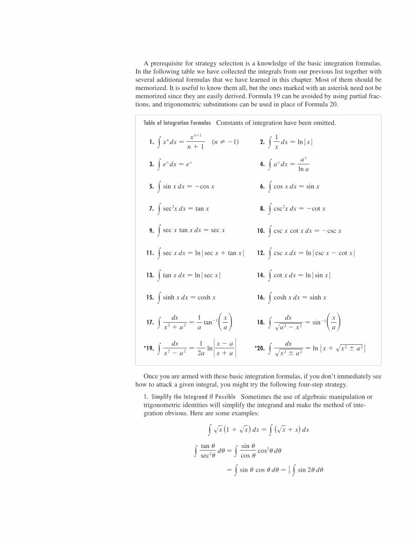
A prerequisite for strategy selection is a knowledge of the basic integration formulas.In the following table we have collected the integrals from our previous list together withseveral additional formulas that we have learned in this chapter. Most of them should bememorized. It is useful to know them all, but the ones marked with an asterisk need not bememorized since they are easily derived. Formula 19 can be avoided by using partial frac-tions, and trigonometric substitutions can be used in place of Formula 20.
Table of Integration Formulas Constants of integration have been omitted.
1. 2.
3. 4.
5. 6.
7. 8.
9. 10.
11. 12.
13. 14.
15. 16.
17. 18.
*19. *20.
Once you are armed with these basic integration formulas, if you don’t immediately seehow to attack a given integral, you might try the following four-step strategy.
1. Simplify the Integrand if Possible Sometimes the use of algebraic manipulation ortrigonometric identities will simplify the integrand and make the method of inte-gration obvious. Here are some examples:
� y sin � cos � d� � 12 y sin 2� d�
y tan �
sec2� d� � y
sin �
cos � cos2� d�
y sx (1 � sx) dx � y (sx � x) dx
y dx
sx 2 � a 2� ln x � sx 2 � a 2 y
dx
x 2 � a 2 �1
2a ln x � a
x � a y
dx
sa 2 � x 2� sin�1� x
a�y dx
x 2 � a 2 �1
a tan�1� x
a�y cosh x dx � sinh xy sinh x dx � cosh x
y cot x dx � ln sin x y tan x dx � ln sec x
y csc x dx � ln csc x � cot x y sec x dx � ln sec x � tan x
y csc x cot x dx � �csc xy sec x tan x dx � sec x
y csc2x dx � �cot xy sec2x dx � tan x
y cos x dx � sin xy sin x dx � �cos x
y ax dx �ax
ln ay ex dx � ex
y 1
x dx � ln x �n � �1�y xn dx �
xn�1
n � 1
2. Look for an Obvious Substitution Try to find some function in the inte-grand whose differential also occurs, apart from a constant factor.For instance, in the integral
we notice that if , then . Therefore, we use the substitu-tion instead of the method of partial fractions.
3. Classify the Integrand According to Its Form If Steps 1 and 2 have not led to thesolution, then we take a look at the form of the integrand .(a) Trigonometric functions. If is a product of powers of and ,
of and , or of and , then we use the substitutions recom-mended in Section 7.2.
(b) Rational functions. If is a rational function, we use the procedure of Sec-tion 7.4 involving partial fractions.
(c) Integration by parts. If is a product of a power of (or a polynomial)and a transcendental function (such as a trigonometric, exponential, or loga-rithmic function), then we try integration by parts, choosing and accord-ing to the advice given in Section 7.1. If you look at the functions in Exer-cises 7.1, you will see that most of them are the type just described.
(d) Radicals. Particular kinds of substitutions are recommended when certainradicals appear.(i) If occurs, we use a trigonometric substitution according to the
table in Section 7.3.(ii) If occurs, we use the rationalizing substitution .
More generally, this sometimes works for .
4. Try Again If the first three steps have not produced the answer, remember thatthere are basically only two methods of integration: substitution and parts.(a) Try substitution. Even if no substitution is obvious (Step 2), some inspiration
or ingenuity (or even desperation) may suggest an appropriate substitution.(b) Try parts. Although integration by parts is used most of the time on products
of the form described in Step 3(c), it is sometimes effective on single func-tions. Looking at Section 7.1, we see that it works on , , and ,and these are all inverse functions.
(c) Manipulate the integrand. Algebraic manipulations (perhaps rationalizing thedenominator or using trigonometric identities) may be useful in transformingthe integral into an easier form. These manipulations may be more substantialthan in Step 1 and may involve some ingenuity. Here is an example:
� y 1 � cos x
sin2x dx � y �csc2x �
cos x
sin2x� dx
y dx
1 � cos x� y
1
1 � cos x�
1 � cos x
1 � cos x dx � y
1 � cos x
1 � cos2x dx
ln xsin�1xtan�1x
sn
t�x�u � s
n ax � bsn ax � b
s�x 2 � a 2
dvu
xf �x�
f
csc xcot xsec xtan xcos xsin xf �x�
f �x�
u � x 2 � 1du � 2x dxu � x 2 � 1
y x
x 2 � 1 dx
du � t��x� dxu � t�x�
� y �1 � 2 sin x cos x� dx
y �sin x � cos x�2 dx � y �sin2x � 2 sin x cos x � cos2x� dx
SECTION 7.5 STRATEGY FOR INTEGRATION ❙ ❙ ❙ ❙ 507

508 ❙ ❙ ❙ ❙ CHAPTER 7 TECHNIQUES OF INTEGRATION
(d) Relate the problem to previous problems. When you have built up some expe-rience in integration, you may be able to use a method on a given integral thatis similar to a method you have already used on a previous integral. Or youmay even be able to express the given integral in terms of a previous one. Forinstance, is a challenging integral, but if we make use of theidentity , we can write
and if has previously been evaluated (see Example 8 in Section 7.2),then that calculation can be used in the present problem.
(e) Use several methods. Sometimes two or three methods are required to evalu-ate an integral. The evaluation could involve several successive substitutions of different types, or it might combine integration by parts with one or moresubstitutions.
In the following examples we indicate a method of attack but do not fully work out theintegral.
EXAMPLE 1
In Step 1 we rewrite the integral:
The integral is now of the form with odd, so we can use the advice inSection 7.2.
Alternatively, if in Step 1 we had written
then we could have continued as follows with the substitution :
EXAMPLE 2
According to Step 3(d)(ii) we substitute . Then , so and
The integrand is now a product of and the transcendental function so it can be inte-grated by parts.
euu
y esx dx � 2 y ueu du
dx � 2u dux � u 2u � sx
y esx dx
� y u 2 � 1
u 6 du � y �u�4 � u�6 � du
y sin3x
cos6x dx � y
1 � cos2x
cos6x sin x dx � y
1 � u 2
u 6 ��du�
u � cos x
y tan3x
cos3x dx � y
sin3x
cos3x
1
cos3x dx � y
sin3x
cos6x dx
mx tanmx secnx dx
y tan3x
cos3x dx � y tan3x sec3x dx
y tan3x
cos3x dx
x sec3x dx
y tan2x sec x dx � y sec3x dx � y sec x dx
tan2x � sec2x � 1x tan2x sec x dx

EXAMPLE 3
No algebraic simplification or substitution is obvious, so Steps 1 and 2 don’t apply here.The integrand is a rational function so we apply the procedure of Section 7.4, remember-ing that the first step is to divide.
EXAMPLE 4
Here Step 2 is all that is needed. We substitute because its differential is, which occurs in the integral.
EXAMPLE 5
Although the rationalizing substitution
works here [Step 3(d)(ii)], it leads to a very complicated rational function. An easiermethod is to do some algebraic manipulation [either as Step 1 or as Step 4(c)]. Multiply-ing numerator and denominator by , we have
C a n W e I n t e g r a t e A l l C o n t i n u o u s F u n c t i o n s ?
The question arises: Will our strategy for integration enable us to find the integral of everycontinuous function? For example, can we use it to evaluate ? The answer is no, atleast not in terms of the functions that we are familiar with.
The functions that we have been dealing with in this book are called elementary func-tions. These are the polynomials, rational functions, power functions , exponentialfunctions , logarithmic functions, trigonometric and inverse trigonometric functions,hyperbolic and inverse hyperbolic functions, and all functions that can be obtained fromthese by the five operations of addition, subtraction, multiplication, division, and compo-sition. For instance, the function
is an elementary function.If is an elementary function, then is an elementary function but need not
be an elementary function. Consider . Since is continuous, its integral exists,and if we define the function by
F�x� � yx
0 e t 2
dt
Fff �x� � ex2
x f �x� dxf �f
f �x� � � x 2 � 1
x 3 � 2x � 1� ln�cosh x� � xe sin 2x
�ax ��xa �
x ex2 dx
� sin�1x � s1 � x 2 � C
� y1
s1 � x 2 dx � y
x
s1 � x 2 dx
y�1 � x
1 � x dx � y
1 � x
s1 � x 2 dx
s1 � x
u � � 1 � x
1 � x
y �1 � x
1 � x dx
du � dx�xu � ln x
y dx
xsln x
y x 5 � 1
x 3 � 3x 2 � 10x dx
SECTION 7.5 STRATEGY FOR INTEGRATION ❙ ❙ ❙ ❙ 509

510 ❙ ❙ ❙ ❙ CHAPTER 7 TECHNIQUES OF INTEGRATION
then we know from Part 1 of the Fundamental Theorem of Calculus that
Thus, has an antiderivative , but it has been proved that is not an elemen-tary function. This means that no matter how hard we try, we will never succeed in evalu-ating in terms of the functions we know. (In Chapter 11, however, we will see howto express as an infinite series.) The same can be said of the following integrals:
In fact, the majority of elementary functions don’t have elementary antiderivatives. Youmay be assured, though, that the integrals in the following exercises are all elementaryfunctions.
y sx 3 � 1 dx y 1
ln x dx y
sin x
x dx
y ex
x dx y sin�x 2 � dx y cos�ex� dx
x ex2 dx
x ex2 dx
FFf �x� � ex2
F��x� � ex2
25. 26.
27. 28.
29. 30.
32.
33. 34.
35. 36.
37. 38.
39. 40.
42.
43. 44.
46.
47. 48. y x
x 4 � a 4 dxy x � a
x 2 � a 2 dx
y 1 � e x
1 � e x dxy x 5e �x 3dx45.
y s1 � e x dxy e xs1 � e x dx
y x 2 tan�1x dxy � tan2� d�41.
y 1
s4y 2 � 4y � 3 dyy
x
1 � x 2 � s1 � x 2 dx
y��4
0 tan5� sec3� d� y
��4
0 cos2� tan2� d�
y sin 4x cos 3x dxy1
�1 x 8 sin x dx
y��2
��4 1 � 4 cot x
4 � cot x dxy s3 � 2x � x 2 dx
y s2x � 1
2x � 3 dxy �1 � x
1 � x dx31.
y2
�2 x 2 � 4x dxy
5
0 3w � 1
w � 2 dw
y sin sat dty cot x ln�sin x� dx
y 3x 2 � 2
x 3 � 2x � 8 dxy
3x 2 � 2
x 2 � 2x � 8 dx
1–80 |||| Evaluate the integral.
1. 2.
3. 4.
6.
7. 8.
9. 10.
11. 12.
13. 14.
15. 16.
18.
19. 20.
21. 22.
24. y ln�x 2 � 1� dxy1
0 (1 � sx )8 dx23.
y x sin�1x dxy t 3e�2 t dt
y e3sx dxy e x�e x
dx
y e2 t
1 � e4 t dty x sin2x dx17.
ys2�2
0
x 2
s1 � x 2 dxy
1�2
0
x
s1 � x 2 dx
y s1 � ln x
x ln x dxy
dx
�1 � x 2�3�2
y sin x cos�cos x� dxy sin3� cos5� d�
y x
x 4 � x 2 � 1 dxy
x � 1
x 2 � 4x � 5 dx
y4
0
x � 1
x 2 � 4x � 5 dxy
3
1 r 4 ln r dr
y x csc x cot x dxy1
�1
e arctan y
1 � y 2 dy5.
y x
s3 � x 4 dxy
2
0
2t
�t � 3�2 dt
y tan3� d�y sin x � sec x
tan x dx
|||| 7.5 Exercises

SECTION 7.6 INTEGRATION USING TABLES AND COMPUTER ALGEBRA SYSTEMS ❙ ❙ ❙ ❙ 511
50.
51. 52.
53. 54.
55. 56.
58.
59. 60.
61. 62.
64.
65. 66. y3
2
u 3 � 1
u 3 � u 2 duy 1
sx � 1 � sx dx
y��3
��4
ln�tan x�sin x cos x
dxy sxesx dx63.
y x 3
�x � 1�10 dxy x 4
x 10 � 16 dx
y 1
x � s3 x
dxy 1
e 3x � e x dx
y x 2 ln�1 � x� dxy xs3 x � c dx57.
y x ln x
sx 2 � 1 dxy
1
x � 4 � 4sx � 1 dx
y �x � sin x�2 dxy x 2 sinh mx dx
y dx
x �x 4 � 1�y 1
xs4x 2 � 1 dx
y 1
x 2s4x � 1
dxy 1
xs4x � 1 dx49. 67. 68.
70.
71. 72.
73. 74.
75. 76.
77. 78.
79. 80.
81. The functions and don’t have elementaryantiderivatives, but does. Evaluate
.x �2x 2 � 1�e x 2 dx
y � �2x 2 � 1�e x 2y � x 2e x 2
y � e x 2
■■ ■■ ■■ ■■ ■■ ■■ ■■ ■■ ■■ ■■ ■■ ■■
y sin x cos x
sin4 x � cos4 x dxy x sin2 x cos x dx
y sec x cos 2x
sin x � sec x dxy
sx
1 � x 3 dx
y �x 2 � bx� sin 2x dxy sin x sin 2x sin 3x dx
y dx
e x � e �xy 1
�x � 2��x 2 � 4� dx
y st
1 � s3 t
dty x
x 4 � 4x 2 � 3 dx
y ln�x � 1�
x 2 dxy e 2x
1 � e x dx69.
y 1
1 � 2e x � e�x dxy3
1 arctanst
st dt
|||| 7.6 I n t e g r a t i o n U s i n g T a b l e s a n d C o m p u t e r A l g e b r a S y s t e m s
In this section we describe how to use tables and computer algebra systems to integratefunctions that have elementary antiderivatives. You should bear in mind, though, that eventhe most powerful computer algebra systems can’t find explicit formulas for the antideriv-atives of functions like or the other functions described at the end of Section 7.5.
T a b l e s o f I n t e g r a l s
Tables of indefinite integrals are very useful when we are confronted by an integral that isdifficult to evaluate by hand and we don’t have access to a computer algebra system. A rel-atively brief table of 120 integrals, categorized by form, is provided on the Reference Pagesat the back of the book. More extensive tables are available in CRC Standard Mathe-matical Tables and Formulae, 30th ed. by Daniel Zwillinger (Boca Raton, FL: CRC Press, 1995) (581 entries) or in Gradshteyn and Ryzhik’s Table of Integrals, Series,and Products, 6e (New York: Academic Press, 2000), which contains hundreds of pages ofintegrals. It should be remembered, however, that integrals do not often occur in exactlythe form listed in a table. Usually we need to use substitution or algebraic manipulation totransform a given integral into one of the forms in the table.
EXAMPLE 1 The region bounded by the curves , and is rotatedabout the -axis. Find the volume of the resulting solid.
SOLUTION Using the method of cylindrical shells, we see that the volume is
V � y1
0 2�x arctan x dx
yx � 1y � arctan x, y � 0
ex 2

512 ❙ ❙ ❙ ❙ CHAPTER 7 TECHNIQUES OF INTEGRATION
In the section of the Table of Integrals entitled Inverse Trigonometric Forms we locateFormula 92:
Thus, the volume is
EXAMPLE 2 Use the Table of Integrals to find .
SOLUTION If we look at the section of the table entitled Forms involving , we seethat the closest entry is number 34:
This is not exactly what we have, but we will be able to use it if we first make the substi-tution :
Then we use Formula 34 with (so ):
EXAMPLE 3 Use the Table of Integrals to find .
SOLUTION If we look in the section called Trigonometric Forms, we see that none of the entries explicitly includes a factor. However, we can use the reduction formula in entry 84 with :
We now need to evaluate . We can use the reduction formula in entry 85with , followed by entry 82:
� x 2 sin x � 2�sin x � x cos x� � K
y x 2 cos x dx � x 2 sin x � 2 y x sin x dx
n � 2x x 2 cos x dx
y x 3 sin x dx � �x 3 cos x � 3 y x 2 cos x dx
n � 3u 3
y x 3 sin x dx
� �x
8 s5 � 4x 2 �
5
16 sin�1� 2x
s5� � C
y x 2
s5 � 4x 2 dx �
1
8 y
u 2
s5 � u 2 du �
1
8 ��
u
2 s5 � u 2 �
5
2 sin�1
u
s5� � C
a � s5a 2 � 5
y x 2
s5 � 4x 2 dx � y
�u�2�2
s5 � u 2 du
2�
1
8 y
u 2
s5 � u 2 du
u � 2x
y u 2
sa 2 � u 2 du � �
u
2 sa 2 � u 2 �
a 2
2 sin�1�u
a� � C
sa 2 � u 2
y x 2
s5 � 4x 2 dx
� � �2���4� � 1� � 12 � 2 � �
� � ��x 2 � 1� tan�1x � x�01 � � �2 tan�1 1 � 1�
V � 2� y1
0 x tan�1x dx � 2�� x 2 � 1
2tan�1x �
x
2 0
1
y u tan�1u du �u 2 � 1
2 tan�1u �
u
2� C
|||| The Table of Integrals appears on the Reference Pages at the back of the book.
85.
� u n sin u � n y u n�1 sin u du
y u n cos u du

Combining these calculations, we get
where .
EXAMPLE 4 Use the Table of Integrals to find .
SOLUTION Since the table gives forms involving , , and , butnot , we first complete the square:
If we make the substitution (so ), the integrand will involve thepattern :
The first integral is evaluated using the substitution :
For the second integral we use Formula 21 with :
Thus
C o m p u t e r A l g e b r a S y s t e m s
We have seen that the use of tables involves matching the form of the given integrand withthe forms of the integrands in the tables. Computers are particularly good at matching pat-terns. And just as we used substitutions in conjunction with tables, a CAS can perform sub-stitutions that transform a given integral into one that occurs in its stored formulas. So itisn’t surprising that computer algebra systems excel at integration. That doesn’t mean thatintegration by hand is an obsolete skill. We will see that a hand computation sometimesproduces an indefinite integral in a form that is more convenient than a machine answer.
To begin, let’s see what happens when we ask a machine to integrate the relatively simple function . Using the substitution , an easy calculationby hand gives
y 1
3x � 2 dx � 1
3 ln 3x � 2 � C
u � 3x � 2y � 1��3x � 2�
� 13�x 2 � 2x � 4�3�2 �
x � 1
2 sx 2 � 2x � 4 �
32 ln(x � 1 � sx 2 � 2x � 4 ) � C
y xsx 2 � 2x � 4 dx
y su 2 � 3 du �u
2 su 2 � 3 �
32 ln(u � su 2 � 3)
a � s3
y usu 2 � 3 du � 12 y st dt � 1
2 � 23 t 3�2 � 1
3 �u 2 � 3�3�2
t � u 2 � 3
� y usu 2 � 3 du � y su 2 � 3 du
y xsx 2 � 2x � 4 dx � y �u � 1� su 2 � 3 du
sa 2 � u 2
x � u � 1u � x � 1
x 2 � 2x � 4 � �x � 1�2 � 3
sax 2 � bx � csx 2 � a 2
sa 2 � x 2sa 2 � x 2
y xsx 2 � 2x � 4 dx
C � 3K
y x 3 sin x dx � �x 3 cos x � 3x 2 sin x � 6x cos x � 6 sin x � C
SECTION 7.6 INTEGRATION USING TABLES AND COMPUTER ALGEBRA SYSTEMS ❙ ❙ ❙ ❙ 513
21.
�a 2
2 ln(u � sa 2 � u 2 ) � C
y sa 2 � u 2 du �u
2 sa 2 � u 2
514 ❙ ❙ ❙ ❙ CHAPTER 7 TECHNIQUES OF INTEGRATION
whereas Derive, Mathematica, and Maple all return the answer
The first thing to notice is that computer algebra systems omit the constant of integra-tion. In other words, they produce a particular antiderivative, not the most general one.Therefore, when making use of a machine integration, we might have to add a constant.Second, the absolute value signs are omitted in the machine answer. That is fine if ourproblem is concerned only with values of greater than . But if we are interested in othervalues of , then we need to insert the absolute value symbol.
In the next example we reconsider the integral of Example 4, but this time we ask amachine for the answer.
EXAMPLE 5 Use a computer algebra system to find .
SOLUTION Maple responds with the answer
This looks different from the answer we found in Example 4, but it is equivalent becausethe third term can be rewritten using the identity
Thus
The resulting extra term can be absorbed into the constant of integration.Mathematica gives the answer
Mathematica combined the first two terms of Example 4 (and the Maple result) into asingle term by factoring.
Derive gives the answer
The first term is like the first term in the Mathematica answer, and the second term isidentical to the last term in Example 4.
EXAMPLE 6 Use a CAS to evaluate .
SOLUTION Maple and Mathematica give the same answer:
118 x
18 �52 x
16 � 50x 14 �1750
3 x 12 � 4375x 10 � 21875x 8 �218750
3 x 6 � 156250x 4 �390625
2 x 2
y x�x 2 � 5�8 dx
16 sx 2 � 2x � 4 �2x 2 � x � 5� �
32 ln(sx 2 � 2x � 4 � x � 1)
�5
6�
x
6�
x 2
3 � sx 2 � 2x � 4 �3
2 arcsinh�1 � x
s3 ��
32 ln(1�s3)
� ln 1
s3� ln(x � 1 � sx 2 � 2x � 4)
� ln 1
s3 [1 � x � s�1 � x�2 � 3]
arcsinh s3
3 �1 � x� � ln�s3
3 �1 � x� � s|
13 �1 � x�2 � 1�
arcsinh x � ln(x � sx 2 � 1)
13 �x 2 � 2x � 4�3�2 �
14 �2x � 2�sx 2 � 2x � 4 �
3
2 arcsinh
s3
3 �1 � x�
y xsx 2 � 2x � 4 dx
x
23x
13 ln�3x � 2�
|||| This is Equation 3.9.3.

SECTION 7.6 INTEGRATION USING TABLES AND COMPUTER ALGEBRA SYSTEMS ❙ ❙ ❙ ❙ 515
It’s clear that both systems must have expanded by the Binomial Theorem andthen integrated each term.
If we integrate by hand instead, using the substitution , we get
For most purposes, this is a more convenient form of the answer.
EXAMPLE 7 Use a CAS to find .
SOLUTION In Example 2 in Section 7.2 we found that
Derive and Maple report the answer
whereas Mathematica produces
We suspect that there are trigonometric identities which show these three answers areequivalent. Indeed, if we ask Derive, Maple, and Mathematica to simplify their expres-sions using trigonometric identities, they ultimately produce the same form of the answeras in Equation 1.
EXAMPLE 8 If , find the antiderivative F of f such that Graph for . Where does have extreme values and inflection points?
SOLUTION The antiderivative of produced by Maple is
and we note that . This expression could probably be simplified, but there’s noneed to do so because a computer algebra system can graph this version of as easily asany other version. A graph of is shown in Figure 1. To locate the extreme values of ,we graph its derivative in Figure 2 and observe that F has a local maximumwhen and a local minimum when . The graph of in Figure 2shows that F has inflection points when , 1.3, 1.8, 2.4, 3.3, and 3.9.x 0.7
F � � f �x 2.5x 2.3F� � f
FFF
F�0� � 0
F�x� � 12 x
2 �203 sin3x cos6x �
207 sin x cos6x �
47 cos4x sin x �
1621 cos2x sin x �
3221 sin x
f
F0 � x � 5FF�0� � 0.f �x� � x � 60 sin4x cos5x
�564 cos x �
1192 cos 3x �
3320 cos 5x �
1448 cos 7x
�17 sin4x cos3x �
435 sin2x cos3x �
8105 cos3x
y sin5x cos2x dx � �13 cos3x �
25 cos5x �
17 cos7x � C1
y sin5x cos2x dx
y x�x 2 � 5�8 dx � 118 �x 2 � 5�9 � C
u � x 2 � 5
�x 2 � 5�8
|||| Derive and the TI-89/92 also give this answer.
50
10
F
FIGURE 1
_7
0 5
10
F ffª
FIGURE 2
3. ; entry 71
4. ; entry 98
■■ ■■ ■■ ■■ ■■ ■■ ■■ ■■ ■■ ■■ ■■ ■■
y e 2� sin 3� d�
y sec3��x� dx1–4 |||| Use the indicated entry in the Table of Integrals on the Reference Pages to evaluate the integral.
1. ; entry 33 2. ; entry 55y 3x
s3 � 2x dxy
s7 � 2x 2
x 2 dx
|||| 7.6 Exercises

35–42 |||| Use a computer algebra system to evaluate the integral.Compare the answer with the result of using tables. If the answersare not the same, show that they are equivalent.
35. 36.
37. 38.
39. 40.
41. 42.
43. Computer algebra systems sometimes need a helping handfrom human beings. Ask your CAS to evaluate
If it doesn’t return an answer, ask it to try
instead. Why do you think it was successful with this form ofthe integrand?
44. Try to evaluate
with a computer algebra system. If it doesn’t return an answer,make a substitution that changes the integral into one that theCAS can evaluate.
45–48 |||| Use a CAS to find an antiderivative of such that . Graph and and locate approximately the -coordinates of the extreme points and inflection points of .
45.
46.
47. ,
48.
■■ ■■ ■■ ■■ ■■ ■■ ■■ ■■ ■■ ■■ ■■ ■■
f �x� �x 3 � x
x 6 � 1
0 � x � �f �x� � sin4x cos6x
f �x� � xe�x sin x, �5 � x � 5
f �x� �x 2 � 1
x 4 � x 2 � 1
FxFfF�0� � 0
fFCAS
y �1 � ln x� s1 � �x ln x�2 dx
CAS
y 2xs2 2x � 1 dx
y 2x s4 x � 1 dx
CAS
■■ ■■ ■■ ■■ ■■ ■■ ■■ ■■ ■■ ■■ ■■ ■■
y x 5sx 2 � 1 dxy tan5x dx
y sin4x dxy xs1 � 2x dx
y tan2x sec4x dxy sin3x cos2x dx
y x 2�1 � x 3 �4 dxy x 2s5 � x 2 dx
CAS
516 ❙ ❙ ❙ ❙ CHAPTER 7 TECHNIQUES OF INTEGRATION
5–30 |||| Use the Table of Integrals on the Reference Pages to evaluate the integral.
5. 6.
7. 8.
9.
11. 12.
13. 14.
15. 16.
18.
20.
21. 22.
23. 24.
25.
28.
30.
31. Find the volume of the solid obtained when the region underthe curve , , is rotated about the -axis.
32. The region under the curve from 0 to is rotatedabout the -axis. Find the volume of the resulting solid.
Verify Formula 53 in the Table of Integrals (a) by differentiationand (b) by using the substitution .
34. Verify Formula 31 (a) by differentiation and (b) by substituting.u � a sin �
t � a � bu33.
x��4y � tan2x
y0 � x � 2y � xs4 � x 2
■■ ■■ ■■ ■■ ■■ ■■ ■■ ■■ ■■ ■■ ■■ ■■
y sec2� tan2�
s9 � tan2� d�y
x 4 dx
sx 10 � 229.
y e t sin�t � 3� dty se 2x � 1 dx27.
y1
0 x 4e�x dx26.y
s4 � �ln x�2
x dx
y sin6 2x dxy sec5x dx
y2
0 x 3
s4x 2 � x 4 dxy e x
3 � e2x dx
y dx
e x�1 � 2e x �y sin2x cos x ln�sin x� dx19.
y x 5
x 2 � s2 dxy ys6 � 4y � 4y2 dy17.
y x sin�x 2� cos�3x 2� dxy e x sech�e x � dx
y sin�1sx dxy
tan3�1�z�z 2 dz
y�
0 x 2 cos 3x dxy
0
�1 t 2e�t dt
y s2y 2 � 3
y 2 dy10.y dx
x 2s4x 2 � 9
y csc3�x�2� dxy e�3x cos 4x dx
y3
2
1
x 2s4x 2 � 7
dxy1
0 2x cos�1x dx

DISCOVERY PROJECT PATTERNS IN INTEGRALS ❙ ❙ ❙ ❙ 517
Patterns in Integrals
In this project a computer algebra system is used to investigate indefinite integrals of families offunctions. By observing the patterns that occur in the integrals of several members of the family,you will first guess, and then prove, a general formula for the integral of any member of thefamily.
1. (a) Use a computer algebra system to evaluate the following integrals.
(i) (ii)
(iii) (iv)
(b) Based on the pattern of your responses in part (a), guess the value of the integral
if . What if ?(c) Check your guess by asking your CAS to evaluate the integral in part (b). Then prove it
using partial fractions.
2. (a) Use a computer algebra system to evaluate the following integrals.
(i) (ii) (iii)
(b) Based on the pattern of your responses in part (a), guess the value of the integral
(c) Check your guess with a CAS. Then prove it using the techniques of Section 7.2. Forwhat values of and is it valid?
3. (a) Use a computer algebra system to evaluate the following integrals.
(i) (ii) (iii)
(iv) (v)
(b) Based on the pattern of your responses in part (a), guess the value of
(c) Use integration by parts to prove the conjecture that you made in part (b). For whatvalues of is it valid?
4. (a) Use a computer algebra system to evaluate the following integrals.
(i) (ii) (iii)
(iv) (v)
(b) Based on the pattern of your responses in part (a), guess the value of . Then useyour CAS to check your guess.
(c) Based on the patterns in parts (a) and (b), make a conjecture as to the value of the integral
when is a positive integer.(d) Use mathematical induction to prove the conjecture you made in part (c).
n
y x ne x dx
x x 6e x dx
y x 5e x dxy x 4e x dx
y x 3e x dxy x 2e x dxy xe x dx
n
y x n ln x dx
y x7 ln x dxy x 3 ln x dx
y x 2 ln x dxy x ln x dxy ln x dx
ba
y sin ax cos bx dx
y sin 8x cos 3x dxy sin 3x cos 7x dxy sin x cos 2x dx
a � ba � b
y 1
�x � a��x � b� dx
y 1
�x � 2�2 dxy 1
�x � 2��x � 5� dx
y 1
�x � 1��x � 5� dxy
1
�x � 2��x � 3� dx
CAS
DISCOVERY PROJECT

518 ❙ ❙ ❙ ❙ CHAPTER 7 TECHNIQUES OF INTEGRATION
|||| 7.7 A p p r o x i m a t e I n t e g r a t i o n
There are two situations in which it is impossible to find the exact value of a definite integral.
The first situation arises from the fact that in order to evaluate using theFundamental Theorem of Calculus we need to know an antiderivative of . Sometimes,however, it is difficult, or even impossible, to find an antiderivative (see Section 7.5). Forexample, it is impossible to evaluate the following integrals exactly:
The second situation arises when the function is determined from a scientific experi-ment through instrument readings or collected data. There may be no formula for the func-tion (see Example 5).
In both cases we need to find approximate values of definite integrals. We already knowone such method. Recall that the definite integral is defined as a limit of Riemann sums,so any Riemann sum could be used as an approximation to the integral: If we divide into subintervals of equal length , then we have
where is any point in the th subinterval . If is chosen to be the left endpointof the interval, then and we have
If , then the integral represents an area and (1) represents an approximation of thisarea by the rectangles shown in Figure 1(a). If we choose to be the right endpoint, then
and we have
[See Figure 1(b).] The approximations and defined by Equations 1 and 2 are calledthe left endpoint approximation and right endpoint approximation, respectively.
In Section 5.2 we also considered the case where is chosen to be the midpoint ofthe subinterval . Figure 1(c) shows the midpoint approximation , which appearsto be better than either or .
Midpoint Rule
and xi � 12 �xi�1 � xi � � midpoint of xi�1, xi�
x �b � a
nwhere
yb
a f �x� dx Mn � x f �x1� � f �x2 � � � � � � f �xn ��
RnLn
Mnxi�1, xi�xix i*
RnLn
yb
a f �x� dx Rn � �
n
i�1 f �xi � x2
x i* � xi
x i*f �x� � 0
yb
a f �x� dx Ln � �
n
i�1 f �xi�1� x1
x i* � xi�1
x i*xi�1, xi�ix i*
yb
a f �x� dx �
n
i�1 f �xi*� x
x � �b � a��nna, b�
y1
�1 s1 � x 3 dxy
1
0 ex2
dx
fx
ba f �x� dx
– – –x™ x£ x¢–x¡
(a) Left endpoint approximation
y
x¸ ⁄ x™ x£ x¢ x0
(b) Right endpoint approximation
y
x¸ ⁄ x™ x£ x¢ x0
x
(c) Midpoint approximation
y
0
FIGURE 1

SECTION 7.7 APPROXIMATE INTEGRATION ❙ ❙ ❙ ❙ 519
Another approximation, called the Trapezoidal Rule, results from averaging the approx-imations in Equations 1 and 2:
Trapezoidal Rule
where and .
The reason for the name Trapezoidal Rule can be seen from Figure 2, which illustratesthe case . The area of the trapezoid that lies above the th subinterval is
and if we add the areas of all these trapezoids, we get the right side of the TrapezoidalRule.
EXAMPLE 1 Use (a) the Trapezoidal Rule and (b) the Midpoint Rule with toapproximate the integral .
SOLUTION(a) With , and , we have , and so the Trape-zoidal Rule gives
This approximation is illustrated in Figure 3.
(b) The midpoints of the five subintervals are , , , , and , so the MidpointRule gives
This approximation is illustrated in Figure 4.
0.691908
�1
5 � 1
1.1�
1
1.3�
1
1.5�
1
1.7�
1
1.9� y
2
1 1
x dx x f �1.1� � f �1.3� � f �1.5� � f �1.7� � f �1.9��
1.91.71.51.31.1
0.695635
� 0.1�1
1�
2
1.2�
2
1.4�
2
1.6�
2
1.8�
1
2� y
2
1 1
x dx T5 �
0.2
2 f �1� � 2 f �1.2� � 2 f �1.4� � 2 f �1.6� � 2 f �1.8� � f �2��
x � �2 � 1��5 � 0.2b � 2n � 5, a � 1
x21 �1�x� dx
n � 5
x � f �xi�1� � f �xi�2 � �
x
2 f �xi�1� � f �xi��
if �x� � 0
xi � a � i xx � �b � a��n
yb
a f �x� dx Tn �
x
2 f �x0 � � 2 f �x1� � 2 f �x2 � � � � � � 2 f �xn�1� � f �xn ��
�x
2 f �x0 � � 2 f �x1� � 2 f �x2 � � � � � � 2 f �xn�1� � f �xn ��
�x
2 � f �x0 � � f �x1�� � � f �x1� � f �x2 �� � � � � � � f �xn�1� � f �xn ���
yb
a f �x� dx
1
2 ��n
i�1 f �xi�1 � x � �
n
i�1 f �xi� x� �
x
2 ��
n
i�1 � f �xi�1 � � f �xi���
FIGURE 3
0
y
xx¸ ⁄ x™ x¢x£
FIGURE 2Trapezoidal approximation
FIGURE 4
1xy=
1 2
1xy=
1 2

520 ❙ ❙ ❙ ❙ CHAPTER 7 TECHNIQUES OF INTEGRATION
In Example 1 we deliberately chose an integral whose value can be computed explic-itly so that we can see how accurate the Trapezoidal and Midpoint Rules are. By theFundamental Theorem of Calculus,
The error in using an approximation is defined to be the amount that needs to be added tothe approximation to make it exact. From the values in Example 1 we see that the errorsin the Trapezoidal and Midpoint Rule approximations for are
In general, we have
The following tables show the results of calculations similar to those in Example 1, butfor , and and for the left and right endpoint approximations as well as theTrapezoidal and Midpoint Rules.
We can make several observations from these tables:
1. In all of the methods we get more accurate approximations when we increase thevalue of . (But very large values of result in so many arithmetic operations thatwe have to beware of accumulated round-off error.)
2. The errors in the left and right endpoint approximations are opposite in sign andappear to decrease by a factor of about 2 when we double the value of .
3. The Trapezoidal and Midpoint Rules are much more accurate than the endpointapproximations.
4. The errors in the Trapezoidal and Midpoint Rules are opposite in sign and appearto decrease by a factor of about 4 when we double the value of .
5. The size of the error in the Midpoint Rule is about half the size of the error in theTrapezoidal Rule.
Figure 5 shows why we can usually expect the Midpoint Rule to be more accurate thanthe Trapezoidal Rule. The area of a typical rectangle in the Midpoint Rule is the same asthe trapezoid whose upper side is tangent to the graph at . The area of this trape-zoid is closer to the area under the graph than is the area of the trapezoid used inAQRD
PABCD
n
n
nn
20n � 5, 10
EM � yb
a f �x� dx � MnandET � y
b
a f �x� dx � Tn
EM 0.001239andET �0.002488
n � 5
y2
1 1
x dx � ln x]1
2� ln 2 � 0.693147 . . .
n
5 0.745635 0.645635 0.695635 0.69190810 0.718771 0.668771 0.693771 0.69283520 0.705803 0.680803 0.693303 0.693069
MnTnRnLn
n
5 �0.052488 0.047512 �0.002488 0.00123910 �0.025624 0.024376 �0.000624 0.00031220 �0.012656 0.012344 �0.000156 0.000078
EMETEREL
yb
a f �x� dx � approximation � error
Approximations to y2
1 1
x dx
Corresponding errors
|||| It turns out that these observations are truein most cases.
Module 5.1/5.2/7.7 allows you to com-pare approximation methods.

the Trapezoidal Rule. [The midpoint error (shaded red) is smaller than the trapezoidal error(shaded blue).]
These observations are corroborated in the following error estimates, which are provedin books on numerical analysis. Notice that Observation 4 corresponds to the in eachdenominator because . The fact that the estimates depend on the size of thesecond derivative is not surprising if you look at Figure 5, because measures howmuch the graph is curved. [Recall that measures how fast the slope of changes.]
Error Bounds Suppose for . If and are the errorsin the Trapezoidal and Midpoint Rules, then
Let’s apply this error estimate to the Trapezoidal Rule approximation in Example 1. If, then and . Since , we have , so
Therefore, taking , and in the error estimate (3), we see that
Comparing this error estimate of with the actual error of about , we seethat it can happen that the actual error is substantially less than the upper bound for theerror given by (3).
EXAMPLE 2 How large should we take in order to guarantee that the Trapezoidal andMidpoint Rule approximations for are accurate to within ?
SOLUTION We saw in the preceding calculation that for , so we cantake , , and in (3). Accuracy to within means that the size ofthe error should be less than . Therefore, we choose so that
Solving the inequality for , we get
or
Thus, will ensure the desired accuracy.n � 41
n 1
s0.0006 40.8
n 2 2
12�0.0001�
n
2�1�3
12n 2 � 0.0001
n0.00010.0001b � 2a � 1K � 2
1 � x � 2 f ��x� � 2
0.0001x21 �1�x� dx
n
0.0024880.006667
ET �2�2 � 1�3
12�5�2 �1
150 0.006667
n � 5K � 2, a � 1, b � 2
f ��x� � � 2
x 3 � �2
13 � 2
1�x � 11 � x � 2f ��x� � 2�x 3f ��x� � �1�x 2f �x� � 1�x
EM �K�b � a�3
24n 2and ET �K�b � a�3
12n 2
EMETa � x � b f ��x� � K3
y � f �x�f ��x�f ��x�
�2n�2 � 4n 2n 2
SECTION 7.7 APPROXIMATE INTEGRATION ❙ ❙ ❙ ❙ 521
FIGURE 5
C
xi
P
DA
B
x–ixi-1
C
P
DA
B
R
Q
|||| It’s quite possible that a lower value for would suffice, but is the smallest value forwhich the error bound formula can guarantee usaccuracy to within .0.0001
41n
|||| can be any number larger than all the values of , but smaller values of give better error bounds.
K f ��x� K

522 ❙ ❙ ❙ ❙ CHAPTER 7 TECHNIQUES OF INTEGRATION
For the same accuracy with the Midpoint Rule we choose so that
which gives
EXAMPLE 3(a) Use the Midpoint Rule with to approximate the integral .(b) Give an upper bound for the error involved in this approximation.
SOLUTION(a) Since , and , the Midpoint Rule gives
Figure 6 illustrates this approximation.
(b) Since , we have and . Also, since, we have and so
Taking , , , and in the error estimate (3), we see that an upperbound for the error is
S i m p s o n ’s R u l e
Another rule for approximate integration results from using parabolas instead of straightline segments to approximate a curve. As before, we divide into subintervals ofequal length , but this time we assume that is an even number. Thenon each consecutive pair of intervals we approximate the curve by a parabolaas shown in Figure 7. If , then is the point on the curve lying above .A typical parabola passes through three consecutive points , and .
0
y
xa=x¸ ⁄ x™ x¢x£ xß=bx∞
P¸ P¡
P™P¢
P£
PßP∞
FIGURE 7
0
y
xh_h
P¸(_h, y¸) P¡(0, ›)
P™(h, fi)
FIGURE 8
Pi�2Pi, Pi�1
xiPi�xi, yi�yi � f �xi�y � f �x� � 0
nh � x � �b � a��nna, b�
6e�1�3
24�10�2 �e
400 0.007
n � 10b � 1a � 0K � 6e
0 � f ��x� � �2 � 4x 2 �ex2� 6e
x 2 � 10 � x � 1f ��x� � �2 � 4x 2 �ex 2
f ��x� � 2xex 2f �x� � ex2
1.460393
� e 0.4225 � e 0.5625 � e 0.7225 � e 0.9025�
� 0.1e 0.0025 � e 0.0225 � e 0.0625 � e 0.1225 � e 0.2025 � e 0.3025
y1
0 ex 2
dx x f �0.05� � f �0.15� � � � � � f �0.85� � f �0.95��
n � 10a � 0, b � 1
x10 ex 2
dxn � 10
n 1
s0.0012 29
2�1�3
24n 2 � 0.0001
n
0
y
x
y=ex2
1
FIGURE 6
|||| Error estimates are upper bounds for the error. They give theoretical, worst-case scenarios. The actual error in this case turns out to be about .0.0023

To simplify our calculations, we first consider the case where , and. (See Figure 8.) We know that the equation of the parabola through , and
is of the form and so the area under the parabola from tois
But, since the parabola passes through , , and , we have
and therefore
Thus, we can rewrite the area under the parabola as
Now, by shifting this parabola horizontally we do not change the area under it. This meansthat the area under the parabola through , and from to in Figure 7is still
Similarly, the area under the parabola through from to is
If we compute the areas under all the parabolas in this manner and add the results, we get
Although we have derived this approximation for the case in which , it is a rea-sonable approximation for any continuous function and is called Simpson’s Rule afterthe English mathematician Thomas Simpson (1710–1761). Note the pattern of coeffi-cients: .1, 4, 2, 4, 2, 4, 2, . . . , 4, 2, 4, 1
ff �x� � 0
�h
3 �y0 � 4y1 � 2y2 � 4y3 � 2y4 � � � � � 2yn�2 � 4yn�1 � yn �
� � � � �h
3 �yn�2 � 4yn�1 � yn �y
b
a f �x� dx
h
3 �y0 � 4y1 � y2 � �
h
3 �y2 � 4y3 � y4 �
h
3 �y2 � 4y3 � y4 �
x � x4x � x2P2, P3, and P4
h
3 �y0 � 4y1 � y2 �
x � x2x � x0P2P0, P1
h
3 �y0 � 4y1 � y2 �
y0 � 4y1 � y2 � 2Ah 2 � 6C
y2 � Ah 2 � Bh � C
y1 � C
y0 � A��h�2 � B��h� � C � Ah 2 � Bh � C
P2�h, y2 �P1�0, y1�P0��h, y0 �
� 2�A h 3
3� Ch� �
h
3 �2Ah 2 � 6C �
� 2�A x 3
3� Cx�
0
h
yh
�h �Ax 2 � Bx � C� dx � 2 y
h
0 �Ax 2 � C � dx
x � hx � �hy � Ax 2 � Bx � C
P2P0, P1x2 � hx0 � �h, x1 � 0
SECTION 7.7 APPROXIMATE INTEGRATION ❙ ❙ ❙ ❙ 523
|||| Here we have used Theorem 5.5.7. Noticethat is even and is odd.BxAx 2 � C

524 ❙ ❙ ❙ ❙ CHAPTER 7 TECHNIQUES OF INTEGRATION
Simpson’s Rule
where is even and .
EXAMPLE 4 Use Simpson’s Rule with to approximate .
SOLUTION Putting , and in Simpson’s Rule, we obtain
Notice that, in Example 4, Simpson’s Rule gives us a much better approximationto the true value of the integral than does the
Trapezoidal Rule or the Midpoint Rule . It turns out(see Exercise 48) that the approximations in Simpson’s Rule are weighted averages ofthose in the Trapezoidal and Midpoint Rules:
(Recall that and usually have opposite signs and is about half the size of .)In many applications of calculus we need to evaluate an integral even if no explicit for-
mula is known for y as a function of x. A function may be given graphically or as a tableof values of collected data. If there is evidence that the values are not changing rapidly,then the Trapezoidal Rule or Simpson’s Rule can still be used to find an approximate valuefor , the integral of y with respect to x.
EXAMPLE 5 Figure 9 shows data traffic on the link from the United States to SWITCH,the Swiss academic and research network, on February 10, 1998. is the datathroughput, measured in megabits per second . Use Simpson’s Rule to estimatethe total amount of data transmitted on the link up to noon on that day.
FIGURE 9 0
2
4
6
D
8
3 6 9 12 15 18 21 24 t (hours)
�Mb�s�D�t�
xba y dx
� ET �� EM �EMET
S2n � 13 Tn �
23 Mn
�M10 � 0.692835��T10 � 0.693771��ln 2 � 0.693147. . .��S10 � 0.693150�
� 0.693150
�0.1
3 �1
1�
4
1.1�
2
1.2�
4
1.3�
2
1.4�
4
1.5�
2
1.6�
4
1.7�
2
1.8�
4
1.9�
1
2� �
�x
3 f �1� � 4 f �1.1� � 2 f �1.2� � 4 f �1.3� � � � � � 2 f �1.8� � 4 f �1.9� � f �2�
y2
1 1
x dx � S10
�x � 0.1f �x� � 1�x, n � 10
x21 �1�x� dxn � 10
�x � �b � a��nn
� 2 f �xn�2 � � 4 f �xn�1� � f �xn �
yb
a f �x� dx � Sn �
�x
3 f �x0 � � 4 f �x1� � 2 f �x2 � � 4 f �x3 � � � � �
|||| Thomas Simpson was a weaver who taughthimself mathematics and went on to become oneof the best English mathematicians of the 18thcentury. What we call Simpson’s Rule was actually known to Cavalieri and Gregory in the17th century, but Simpson popularized it in hisbest-selling calculus textbook, entitled A NewTreatise of Fluxions.

SECTION 7.7 APPROXIMATE INTEGRATION ❙ ❙ ❙ ❙ 525
SOLUTION Because we want the units to be consistent and is measured in megabits per second, we convert the units for from hours to seconds. If we let be the amount of data (in megabits) transmitted by time , where is measured in seconds, then
. So, by the Net Change Theorem (see Section 5.4), the total amount of datatransmitted by noon (when ) is
We estimate the values of at hourly intervals from the graph and compile them inthe table.
Then we use Simpson’s Rule with and to estimate the integral:
Thus, the total amount of data transmitted up to noon is about 144,000 megabits, or 144 gigabits.
In Exercises 27 and 28 you are asked to demonstrate, in particular cases, that the errorin Simpson’s Rule decreases by a factor of about 16 when is doubled. That is consistentwith the appearance of in the denominator of the following error estimate for Simpson’sRule. It is similar to the estimates given in (3) for the Trapezoidal and Midpoint Rules, butit uses the fourth derivative of .
Error Bound for Simpson’s Rule Suppose that for . If is the error involved in using Simpson’s Rule, then
� ES � �K�b � a�5
180n 4
ES
a � x � b� f �4��x� � � K4
f
n 4n
� 143,880
� 2�1.1� � 4�1.3� � 2�2.8� � 4�5.7� � 2�7.1� � 4�7.7� � 7.9
�3600
3 3.2 � 4�2.7� � 2�1.9� � 4�1.7� � 2�1.3� � 4�1.0�
y43,200
0 A�t� dt �
�t
3 D�0� � 4D�3600� � 2D�7200� � � � � � 4D�39,600� � D�43,200�
�t � 3600n � 12
D�t�
A�43,200� � y43,200
0 D�t� dt
t � 12 � 602 � 43,200A��t� � D�t�
ttA�t�t
D�t�
0 0 3.2 7 25,200 1.31 3,600 2.7 8 28,800 2.82 7,200 1.9 9 32,400 5.73 10,800 1.7 10 36,000 7.14 14,400 1.3 11 39,600 7.75 18,000 1.0 12 43,200 7.96 21,600 1.1
D�t�t �seconds�t �hours�D�t�t �seconds�t �hours�

526 ❙ ❙ ❙ ❙ CHAPTER 7 TECHNIQUES OF INTEGRATION
EXAMPLE 6 How large should we take in order to guarantee that the Simpson’s Ruleapproximation for is accurate to within ?
SOLUTION If , then . Since , we have and so
Therefore, we can take in (4). Thus, for an error less than we shouldchoose so that
This gives
or
Therefore, ( must be even) gives the desired accuracy. (Compare this withExample 2, where we obtained for the Trapezoidal Rule and for theMidpoint Rule.)
EXAMPLE 7(a) Use Simpson’s Rule with to approximate the integral .(b) Estimate the error involved in this approximation.
SOLUTION(a) If , then and Simpson’s Rule gives
(b) The fourth derivative of is
and so, since , we have
Therefore, putting , and in (4), we see that the error is atmost
(Compare this with Example 3.) Thus, correct to three decimal places, we have
y1
0 ex 2
dx � 1.463
76e�1�5
180�10�4 � 0.000115
n � 10K � 76e, a � 0, b � 1
0 � f �4��x� � �12 � 48 � 16�e 1 � 76e
0 � x � 1
f �4��x� � �12 � 48x 2 � 16x 4 �ex2
f �x� � ex2
� 1.462681
� 4e 0.49 � 2e 0.64 � 4e 0.81 � e 1
�0.1
3 e 0 � 4e 0.01 � 2e 0.04 � 4e 0.09 � 2e 0.16 � 4e 0.25 � 2e 0.36
y1
0 ex2
dx ��x
3 f �0� � 4 f �0.1� � 2 f �0.2� � � � � � 2 f �0.8� � 4 f �0.9� � f �1�
�x � 0.1n � 10
x10 ex2 dxn � 10
n � 29n � 41nn � 8
n 1
s4 0.00075
� 6.04
n 4 24
180�0.0001�
24�1�5
180n 4 0.0001
n0.0001K � 24
� f �4��x� � � � 24
x 5 � � 24
1�x � 1x � 1f �4��x� � 24�x 5f �x� � 1�x
0.0001x21 �1�x� dx
n
|||| Many calculators and computer algebra sys-tems have a built-in algorithm that computes anapproximation of a definite integral. Some ofthese machines use Simpson’s Rule; others usemore sophisticated techniques such as adaptivenumerical integration. This means that if a func-tion fluctuates much more on a certain part ofthe interval than it does elsewhere, then thatpart gets divided into more subintervals. Thisstrategy reduces the number of calculationsrequired to achieve a prescribed accuracy.
|||| Figure 10 illustrates the calculation inExample 7. Notice that the parabolic arcs are so close to the graph of that they arepractically indistinguishable from it.
y � e x2
0
y
x1
y=e≈
FIGURE 10

SECTION 7.7 APPROXIMATE INTEGRATION ❙ ❙ ❙ ❙ 527
(Round your answers to six decimal places.) Compare your resultsto the actual value to determine the error in each approximation.
5. , 6. ,
7–18 |||| Use (a) the Trapezoidal Rule, (b) the Midpoint Rule, and(c) Simpson’s Rule to approximate the given integral with the specified value of . (Round your answers to six decimal places.)
7. , 8. ,
9. , 10. ,
11. , 12. ,
13. , 14. ,
15. , 16. ,
17. , 18. ,
19. (a) Find the approximations and for the integral.
(b) Estimate the errors in the approximations of part (a).(c) How large do we have to choose so that the approxima-
tions and to the integral in part (a) are accurate towithin ?
20. (a) Find the approximations for .(b) Estimate the errors involved in the approximations of
part (a).(c) How large do we have to choose so that the approxima-
tions and to the integral in part (a) are accurate towithin 0.00001?
21. (a) Find the approximations and for and the corresponding errors and .
(b) Compare the actual errors in part (a) with the error esti-mates given by (3) and (4).
(c) How large do we have to choose so that the approxima-tions , , and to the integral in part (a) are accurate towithin ?
22. How large should be to guarantee that the Simpson’s Ruleapproximation to is accurate to within ?
23. The trouble with the error estimates is that it is often very diffi-cult to compute four derivatives and obtain a good upper bound
for by hand. But computer algebra systems have no� f �4��x� �K
CAS
0.00001x10 ex 2
dxn
0.00001SnMnTn
n
ESET
x10 e x dxS10T10
MnTn
n
x10 cos�x 2 � dxT8 and M8
0.00001MnTn
n
x2
0 e�x 2 dxM10T10
■■ ■■ ■■ ■■ ■■ ■■ ■■ ■■ ■■ ■■ ■■ ■■
n � 10y4
2 e x
x dxn � 6y
3
0
1
1 � y 5 dy
n � 10y6
4 ln�x 3 � 2� dxn � 8y
5
1 cos x
x dx
n � 8y4
0 sx sin x dxn � 4y
2
1 e 1�x dx
n � 8y4
0 s1 � sx dxn � 8y
1�2
0 sin�e t�2 � dt
n � 6y3
0
dt
1 � t 2 � t 4n � 10y2
1
ln x
1 � x dx
n � 4y1�2
0 sin�x 2 � dxn � 8y
2
0 s4 1 � x 2 dx
n
■■ ■■ ■■ ■■ ■■ ■■ ■■ ■■ ■■ ■■ ■■ ■■
n � 6y1
0 e�sx dxn � 8y
�
0 x 2 sin x dx
Let , where is the function whose graph isshown.(a) Use the graph to find .(b) Are these underestimates or overestimates of ?(c) Use the graph to find . How does it compare with ?(d) For any value of , list the numbers and in
increasing order.
2. The left, right, Trapezoidal, and Midpoint Rule approximationswere used to estimate , where is the function whosegraph is shown. The estimates were 0.7811, 0.8675, 0.8632,and 0.9540, and the same number of subintervals were used ineach case.(a) Which rule produced which estimate?(b) Between which two approximations does the true value of
lie?
; Estimate using (a) the Trapezoidal Rule and(b) the Midpoint Rule, each with . From a graph of theintegrand, decide whether your answers are underestimates oroverestimates. What can you conclude about the true value ofthe integral?
; Draw the graph of in the viewing rectangleby and let .
(a) Use the graph to decide whether , and under-estimate or overestimate .
(b) For any value of , list the numbers and inincreasing order.
(c) Compute . From the graph, which do youthink gives the best estimate of ?
5–6 |||| Use (a) the Midpoint Rule and (b) Simpson’s Rule toapproximate the given integral with the specified value of .n
IL5, R5, M5, and T5
ILn, Rn, Mn, Tn,nI
T2L2, R2, M2
I � x10 f �x� dx0, 0.50, 1
f �x� � sin�x 2�2�4.
n � 4x
10 cos�x 2 � dx3.
y
x0
1
2
y=ƒ
x2
0 f �x� dx
fx2
0 f �x� dx
f
x
1
y
2
3
10 2 3 4
ILn, Rn, Mn, Tn,nIT2
IL2, R2, and M2
fI � x40 f �x� dx1.
|||| 7.7 Exercises

528 ❙ ❙ ❙ ❙ CHAPTER 7 TECHNIQUES OF INTEGRATION
problem computing and graphing it, so we can easily find a value for from a machine graph. This exercise deals with approximations to the integral , where
.(a) Use a graph to get a good upper bound for .(b) Use to approximate .(c) Use part (a) to estimate the error in part (b).(d) Use the built-in numerical integration capability of your
CAS to approximate .(e) How does the actual error compare with the error estimate
in part (c)?(f) Use a graph to get a good upper bound for .(g) Use to approximate .(h) Use part (f) to estimate the error in part (g).(i) How does the actual error compare with the error estimate
in part (h)?(j) How large should be to guarantee that the size of the
error in using is less than ?
24. Repeat Exercise 23 for the integral .
25–26 |||| Find the approximations , and for ,and . Then compute the corresponding errors , and .(Round your answers to six decimal places. You may wish to usethe sum command on a computer algebra system.) What observa-tions can you make? In particular, what happens to the errors when
is doubled?
25. 26.
27–28 |||| Find the approximations , , and for and .Then compute the corresponding errors , and . (Roundyour answers to six decimal places. You may wish to use the sumcommand on a computer algebra system.) What observations canyou make? In particular, what happens to the errors when is doubled?
27. 28.
29. Estimate the area under the graph in the figure by using (a) theTrapezoidal Rule, (b) the Midpoint Rule, and (c) Simpson’sRule, each with .
30. The widths (in meters) of a kidney-shaped swimming poolwere measured at 2-meter intervals as indicated in the figure.
0
y
1
x1 2 3 4
n � 4
■■ ■■ ■■ ■■ ■■ ■■ ■■ ■■ ■■ ■■ ■■ ■■
y2
�1 xe x dxy
4
1 sx dx
n
ESET, EM
12n � 6SnMnTn
■■ ■■ ■■ ■■ ■■ ■■ ■■ ■■ ■■ ■■ ■■ ■■
y2
0 e x dxy
1
0 x 3 dx
n
EMEL, ER, ET16n � 4, 8MnLn, Rn, Tn
y1
�1 s4 � x 3 dxCAS
0.0001Sn
n
IS10
� f �4��x� �
I
IM10
� f �x� �f �x� � e cos x
I � x2�
0 f �x� dxK
f �4� Use Simpson’s Rule to estimate the area of the pool.
31. (a) Use the Midpoint Rule and the given data to estimate thevalue of the integral .
(b) If it is known that for all , estimate theerror involved in the approximation in part (a).
32. A radar gun was used to record the speed of a runner duringthe first 5 seconds of a race (see the table). Use Simpson’s Rule to estimate the distance the runner covered during those5 seconds.
The graph of the acceleration of a car measured in isshown. Use Simpson’s Rule to estimate the increase in thevelocity of the car during the 6-second time interval.
34. Water leaked from a tank at a rate of liters per hour, wherethe graph of is as shown. Use Simpson’s Rule to estimate thetotal amount of water that leaked out during the first six hours.
r
t0 642
2
4
rr�t�
a
t0 642
4
8
12
ft�s2a�t�33.
x�4 � f �x� � 1
x3.2
0 f �x� dx
6.2
5.0
7.26.8
5.6 4.84.8
x x
0.0 6.8 2.0 7.60.4 6.5 2.4 8.40.8 6.3 2.8 8.81.2 6.4 3.2 9.01.6 6.9
f �x�f �x�
t (s) (m�s) t (s) (m�s)
0 0 3.0 10.510.5 4.67 3.5 10.671.0 7.34 4.0 10.761.5 8.86 4.5 10.812.0 9.73 5.0 10.812.5 10.22
vv

SECTION 7.7 APPROXIMATE INTEGRATION ❙ ❙ ❙ ❙ 529
39. The region bounded by the curves , , ,and is rotated about the -axis. Use Simpson’s Rule with
to estimate the volume of the resulting solid.
40. The figure shows a pendulum with length that makes a maxi-mum angle with the vertical. Using Newton’s Second Law it can be shown that the period (the time for one completeswing) is given by
where and is the acceleration due to gravity. If m and , use Simpson’s Rule with tofind the period.
41. The intensity of light with wavelength traveling through a diffraction grating with slits at an angle is given by
, where and is the distance between adjacent slits. A helium-neon laser withwavelength is emitting a narrow band oflight, given by , through a grating with10,000 slits spaced apart. Use the Midpoint Rule with
to estimate the total light intensity emerg-ing from the grating.
42. Use the Trapezoidal Rule with to approximate. Compare your result to the actual value. Can
you explain the discrepancy?
43. Sketch the graph of a continuous function on for whichthe Trapezoidal Rule with is more accurate than theMidpoint Rule.
44. Sketch the graph of a continuous function on for whichthe right endpoint approximation with is more accuratethan Simpson’s Rule.
If is a positive function and for , showthat
46. Show that if is a polynomial of degree 3 or lower, then Simpson’s Rule gives the exact value of .
47. Show that .
48. Show that .13 Tn �
23 Mn � S2n
12 �Tn � Mn � � T2n
xba f �x� dx
f
Tn yb
a f �x� dx Mn
a � x � bf �x� 0f45.
n � 20, 2
n � 20, 2
x20
0 cos��x� dxn � 10
x10�6
�10�6 I��� d�n � 1010�4 m
�10�6 � 10�6� � 632.8 � 10�9 m
dk � ��Nd sin ����I��� � N 2 sin2k�k 2�N
�
¨¸
n � 10�0 � 42�L � 1tk � sin( 1
2 �0 )
T � 4�L
t y
��2
0
dx
s1 � k 2 sin2x
T�0
LCAS
n � 10xx � 2
x � 0y � 0y � s3 1 � x 3The table (supplied by San Diego Gas and Electric) gives the
power consumption in megawatts in San Diego County frommidnight to 6:00 A.M. on December 8, 1999. Use Simpson’sRule to estimate the energy used during that time period. (Usethe fact that power is the derivative of energy.)
36. Shown is the graph of traffic on an Internet service provider’sT1 data line from midnight to 8:00 A.M. is the data through-put, measured in megabits per second. Use Simpson’s Rule toestimate the total amount of data transmitted during that timeperiod.
37. If the region shown in the figure is rotated about the -axis toform a solid, use Simpson’s Rule with to estimate thevolume of the solid.
38. The table shows values of a force function where ismeasured in meters and in newtons. Use Simpson’s Ruleto estimate the work done by the force in moving an object adistance of 18 m.
f �x�xf �x�
0 4
4
102 86
2
y
x
n � 8y
0
0.4
4 6
0.8
2 8
D
t (hours)
D
35.
t P t P
0:00 1814 3:30 16110:30 1735 4:00 16211:00 1686 4:30 16661:30 1646 5:00 17452:00 1637 5:30 18862:30 1609 6:00 20523:00 1604
x 0 3 6 9 12 15 18
9.8 9.1 8.5 8.0 7.7 7.5 7.4f �x�

530 ❙ ❙ ❙ ❙ CHAPTER 7 TECHNIQUES OF INTEGRATION
|||| 7.8 I m p r o p e r I n t e g r a l s
In defining a definite integral we dealt with a function defined on a finite inter-val and we assumed that does not have an infinite discontinuity (see Section 5.2).In this section we extend the concept of a definite integral to the case where the interval isinfinite and also to the case where has an infinite discontinuity in . In either casethe integral is called an improper integral. One of the most important applications of thisidea, probability distributions, will be studied in Section 8.5.
T y p e I : I n f i n i t e I n t e r v a l s
Consider the infinite region that lies under the curve , above the -axis, and tothe right of the line . You might think that, since is infinite in extent, its area mustbe infinite, but let’s take a closer look. The area of the part of that lies to the left of theline (shaded in Figure 1) is
Notice that no matter how large is chosen.
We also observe that
The area of the shaded region approaches as (see Figure 2), so we say that the areaof the infinite region is equal to and we write
Using this example as a guide, we define the integral of (not necessarily a positivefunction) over an infinite interval as the limit of integrals over finite intervals.
f
0
y
x1 2
area= 12
0
y
x1 3
area= 23
0
y
x1
area=1
0
y
x1 5
45area=
FIGURE 2
y�
1
1
x 2 dx � limt l �
yt
1
1
x 2 dx � 1
1St l �1
limt l �
A�t� � limt l �
�1 �1
t � � 1
0
y
x1 t
y= 1≈
x=1area=1 - 1
t
FIGURE 1
tA�t� 1
A�t� � yt
1
1
x 2 dx � �1
x 1
t
� 1 �1
t
x � tS
Sx � 1xy � 1�x 2S
a, bf
fa, bfx
ba f �x� dx
Try painting a fence that never ends.Resources / Module 6
/ How To Calculate / Start of Improper Integrals
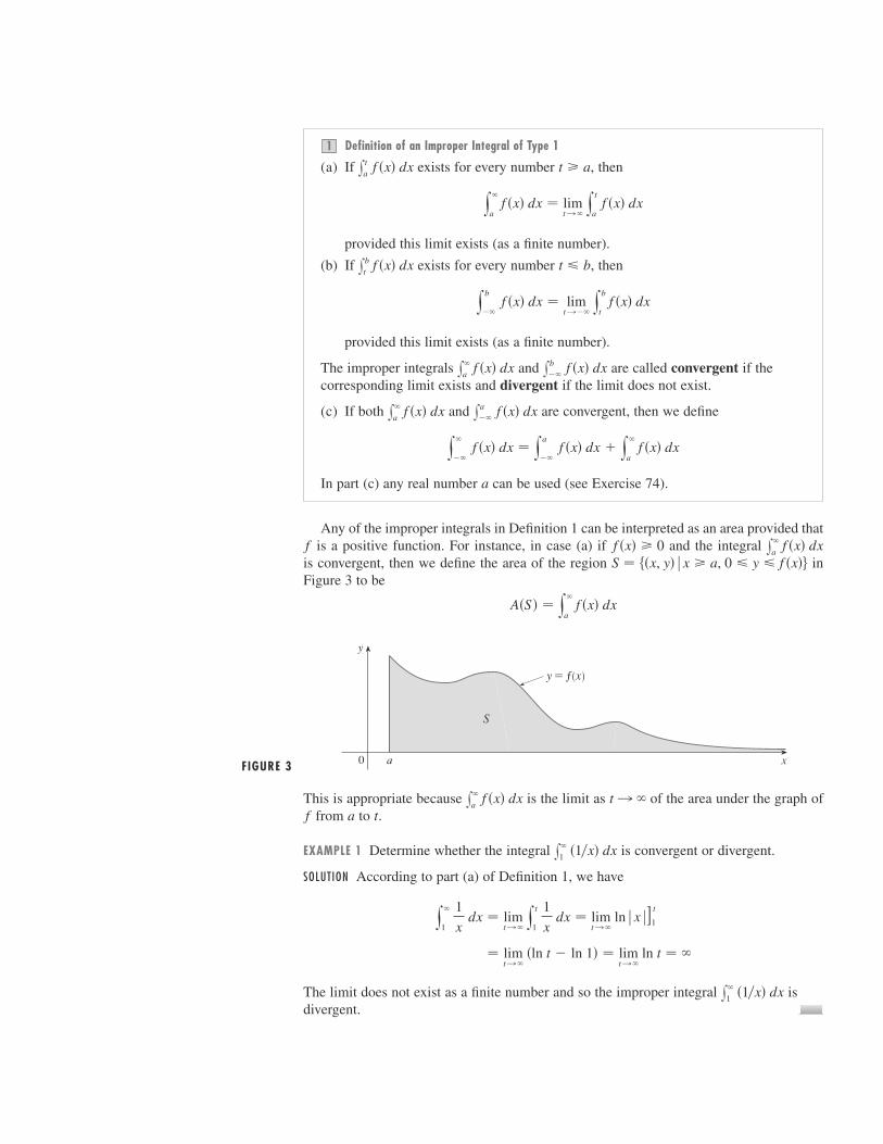
Definition of an Improper Integral of Type 1
(a) If exists for every number , then
provided this limit exists (as a finite number).
(b) If exists for every number , then
provided this limit exists (as a finite number).
The improper integrals and are called convergent if thecorresponding limit exists and divergent if the limit does not exist.
(c) If both and are convergent, then we define
In part (c) any real number can be used (see Exercise 74).
Any of the improper integrals in Definition 1 can be interpreted as an area provided thatis a positive function. For instance, in case (a) if and the integral
is convergent, then we define the area of the region inFigure 3 to be
This is appropriate because is the limit as of the area under the graph offrom to .
EXAMPLE 1 Determine whether the integral is convergent or divergent.
SOLUTION According to part (a) of Definition 1, we have
The limit does not exist as a finite number and so the improper integral isdivergent.
x�
1 �1�x� dx
� limt l �
�ln t � ln 1� � limt l �
ln t � �
y�
1 1
x dx � lim
t l � y
t
1 1
x dx � lim
t l � ln � x �]1
t
x�
1 �1�x� dx
taft l �x
�
a f �x� dx
FIGURE 3 0
y
xa
S
y=ƒ
A�S � � y�
a f �x� dx
S � ��x, y� � x � a, 0 � y � f �x��x
�
a f �x� dxf �x� � 0f
a
y�
�� f �x� dx � y
a
�� f �x� dx � y
�
a f �x� dx
xa��
f �x� dxx�
a f �x� dx
xb��
f �x� dxx�
a f �x� dx
yb
�� f �x� dx � lim
t l�� y
b
t f �x� dx
t � bxbt f �x� dx
y�
a f �x� dx � lim
t l � y
t
a f �x� dx
t � axta f �x� dx
1
SECTION 7.8 IMPROPER INTEGRALS ❙ ❙ ❙ ❙ 531

532 ❙ ❙ ❙ ❙ CHAPTER 7 TECHNIQUES OF INTEGRATION
Let’s compare the result of Example 1 with the example given at the beginning of this section:
Geometrically, this says that although the curves and look very similarfor , the region under to the right of (the shaded region in Figure 4)has finite area whereas the corresponding region under (in Figure 5) has infinitearea. Note that both and approach as but approaches faster than
. The values of 1�x don’t decrease fast enough for its integral to have a finite value.
EXAMPLE 2 Evaluate .
SOLUTION Using part (b) of Definition 1, we have
We integrate by parts with , so that , :
We know that as , and by l’Hospital’s Rule we have
Therefore
EXAMPLE 3 Evaluate .
SOLUTION It’s convenient to choose in Definition 1(c):
We must now evaluate the integrals on the right side separately:
� limt l �
�tan�1t � tan�1 0� � limt l �
tan�1t ��
2
y�
0
1
1 � x 2 dx � limt l �
yt
0
dx
1 � x 2 � limt l �
tan�1x]0
t
y�
��
1
1 � x 2 dx � y0
��
1
1 � x 2 dx � y�
0
1
1 � x 2 dx
a � 0
y�
��
1
1 � x 2 dx
� �0 � 1 � 0 � �1
y0
�� xex dx � lim
t l�� ��te t � 1 � e t�
� lim t l��
��e t� � 0
limt l��
te t � limt l��
t
e�t � limt l��
1
�e�t
t l ��e t l 0
� �te t � 1 � e t
y0
t xex dx � xex]t
0� y
0
t ex dx
v � exdu � dxdv � ex dxu � x
y0
�� xex dx � lim
t l�� y
0
t xex dx
y0
�� xex dx
1�x01�x 2x l �01�x1�x 2
y � 1�xx � 1y � 1�x 2x 0
y � 1�xy � 1�x 2
y�
1 1
x dx divergesy
�
1
1
x 2 dx converges
FIGURE 4
FIGURE 5
infinite area
0
y
x1
y= 1x
0
y
x1
finite area
y= 1≈

Since both of these integrals are convergent, the given integral is convergent and
Since , the given improper integral can be interpreted as the area of the infinite region that lies under the curve and above the -axis (seeFigure 6).
EXAMPLE 4 For what values of is the integral
convergent?
SOLUTION We know from Example 1 that if , then the integral is divergent, so let’sassume that . Then
If , then , so as , and . Therefore
and so the integral converges. But if , then and so
and the integral diverges.
We summarize the result of Example 4 for future reference:
T y p e 2 : D i s c o n t i n u o u s I n t e g r a n d s
Suppose that is a positive continuous function defined on a finite interval but hasa vertical asymptote at . Let be the unbounded region under the graph of and above the -axis between and . (For Type 1 integrals, the regions extended indefinitely in a bax
fSba, b�f
y�
1
1
x p dx is convergent if p 1 and divergent if p � 1.2
as t l �1
t p�1 � t 1�p l �
p � 1 0p 1
if p 1y�
1
1
x p dx �1
p � 1
1�t p�1 l 0t p�1 l �t l �p � 1 0p 1
� limt l �
1
1 � p� 1
t p�1 � 1 � lim
t l �
x�p�1
�p � 1 x�1
x�t
y�
1
1
x p dx � limt l �
yt
1 x�p dx
p � 1p � 1
y�
1
1
x p dx
p
xy � 1��1 � x 2 �1��1 � x 2 � 0
y�
��
1
1 � x 2 dx ��
2�
�
2� �
� 0 � ���
2 � ��
2
� limt l��
�tan�1 0 � tan�1t�
y0
��
1
1 � x 2 dx � limt l��
y0
t
dx
1 � x 2 � limt l��
tan�1x] t
0
SECTION 7.8 IMPROPER INTEGRALS ❙ ❙ ❙ ❙ 533
0
y
x
y= 11+≈
area=π
FIGURE 6
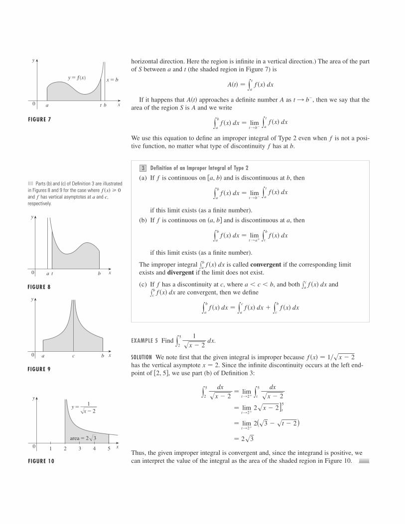
534 ❙ ❙ ❙ ❙ CHAPTER 7 TECHNIQUES OF INTEGRATION
FIGURE 7
0
y
xbta
x=by=ƒ
|||| Parts (b) and (c) of Definition 3 are illustratedin Figures 8 and 9 for the case where and has vertical asymptotes at and ,respectively.
caff �x� � 0
0
y
xa t b
FIGURE 8
0
y
xa c b
FIGURE 9
horizontal direction. Here the region is infinite in a vertical direction.) The area of the partof between and (the shaded region in Figure 7) is
If it happens that approaches a definite number as , then we say that thearea of the region is and we write
We use this equation to define an improper integral of Type 2 even when is not a posi-tive function, no matter what type of discontinuity has at .
Definition of an Improper Integral of Type 2
(a) If is continuous on and is discontinuous at , then
if this limit exists (as a finite number).
(b) If is continuous on and is discontinuous at , then
if this limit exists (as a finite number).
The improper integral is called convergent if the corresponding limitexists and divergent if the limit does not exist.
(c) If has a discontinuity at , where , and both andare convergent, then we define
EXAMPLE 5 Find .
SOLUTION We note first that the given integral is improper because has the vertical asymptote . Since the infinite discontinuity occurs at the left end-point of , we use part (b) of Definition 3:
Thus, the given improper integral is convergent and, since the integrand is positive, wecan interpret the value of the integral as the area of the shaded region in Figure 10.
� 2s3
� limt l2�
2(s3 � st � 2)
� limt l2�
2sx � 2]t
5
y5
2
dx
sx � 2� lim
t l2� y
5
t
dx
sx � 2
�2, 5�x � 2
f �x� � 1�sx � 2
y5
2
1
sx � 2 dx
yb
a f �x� dx � y
c
a f �x� dx � y
b
c f �x� dx
xbc f �x� dx
xca f �x� dxa � c � bcf
xba f �x� dx
yb
a f �x� dx � lim
t l a� y
b
t f �x� dx
a�a, b�f
yb
a f �x� dx � lim
t l b� y
t
a f �x� dx
b�a, b�f
3
bff
yb
a f �x� dx � lim
t l b� y
t
a f �x� dx
ASt l b�AA�t�
A�t� � yt
a f �x� dx
taS
0
y
x1 2 4 53
y= 1œ„„„„x-2
area=2œ„3
FIGURE 10

SECTION 7.8 IMPROPER INTEGRALS ❙ ❙ ❙ ❙ 535
EXAMPLE 6 Determine whether converges or diverges.
SOLUTION Note that the given integral is improper because . Usingpart (a) of Definition 3 and Formula 14 from the Table of Integrals, we have
because and as . Thus, the given improper integral isdivergent.
EXAMPLE 7 Evaluate if possible.
SOLUTION Observe that the line is a vertical asymptote of the integrand. Since itoccurs in the middle of the interval , we must use part (c) of Definition 3 with
:
where
because as . Thus, is divergent. This implies thatis divergent. [We do not need to evaluate .]
| WARNING ■■ If we had not noticed the asymptote in Example 7 and had instead confused the integral with an ordinary integral, then we might have made the followingerroneous calculation:
This is wrong because the integral is improper and must be calculated in terms of limits.From now on, whenever you meet the symbol you must decide, by looking
at the function on , whether it is an ordinary definite integral or an improper integral.
EXAMPLE 8 Evaluate .
SOLUTION We know that the function has a vertical asymptote at 0 since. Thus, the given integral is improper and we have
y1
0 ln x dx � lim
t l 0� y
1
t ln x dx
lim x l 0� ln x � ��f �x� � ln x
y1
0 ln x dx
�a, b�fx
ba f �x� dx
y3
0
dx
x � 1� ln � x � 1 �]3
0 � ln 2 � ln 1 � ln 2
x � 1
x31 dx��x � 1�x
30 dx��x � 1�
x10 dx��x � 1�t l 1�1 � t l 0�
� limt l1�
ln�1 � t� � ��
� limt l1�
(ln � t � 1 � � ln � �1 �) y
1
0
dx
x � 1� lim
t l1� y
t
0
dx
x � 1� lim
t l1� ln � x � 1 �]0
t
y3
0
dx
x � 1� y
1
0
dx
x � 1� y
3
1
dx
x � 1
c � 1�0, 3�
x � 1
y3
0
dx
x � 1
t l ���2��tan t l �sec t l �
� �
� limt l �� /2��
�ln�sec t � tan t� � ln 1�
� limt l �� /2��
ln � sec x � tan x �]0
t
y� /2
0 sec x dx � lim
t l �� /2�� y
t
0 sec x dx
lim x l�� /2�� sec x � �
y� /2
0 sec x dx

536 ❙ ❙ ❙ ❙ CHAPTER 7 TECHNIQUES OF INTEGRATION
Now we integrate by parts with , , , and :
To find the limit of the first term we use l’Hospital’s Rule:
Therefore
Figure 11 shows the geometric interpretation of this result. The area of the shaded regionabove and below the -axis is .
A C o m p a r i s o n T e s t f o r I m p r o p e r I n t e g r a l s
Sometimes it is impossible to find the exact value of an improper integral and yet it is important to know whether it is convergent or divergent. In such cases the following the-orem is useful. Although we state it for Type 1 integrals, a similar theorem is true forType 2 integrals.
Comparison Theorem Suppose that and are continuous functions withfor .
(a) If is convergent, then is convergent.
(b) If is divergent, then is divergent.
We omit the proof of the Comparison Theorem, but Figure 12 makes it seem plausible.If the area under the top curve is finite, then so is the area under the bottom curve
. And if the area under is infinite, then so is the area under .[Note that the reverse is not necessarily true: If is convergent, may or may not be convergent, and if is divergent, may or may not bedivergent.]
EXAMPLE 9 Show that is convergent.
SOLUTION We can’t evaluate the integral directly because the antiderivative of is notan elementary function (as explained in Section 7.5). We write
y�
0 e�x2
dx � y1
0 e�x2 dx � y
�
1 e�x2 dx
e�x2
y�
0 e�x2 dx
x�
a t�x� dxx�
a f �x� dxx
�
a f �x� dxx�
a t�x� dxy � f �x�y � t�x�y � t�x�
y � f �x�
x�
a f �x� dxx�
a t�x� dx
x�
a t�x� dxx�
a f �x� dx
x � af �x� � t�x� � 0tf
1xy � ln x
� �0 � 1 � 0 � �1
y1
0 ln x dx � lim
t l 0� ��t ln t � 1 � t�
� limt l 0�
��t� � 0
� limt l 0�
1�t
�1�t 2
limt l 0�
t ln t � limt l 0�
ln t
1�t
� �t ln t � 1 � t
� 1 ln 1 � t ln t � �1 � t�
y1
t ln x dx � x ln x]t
1� y
1
t dx
v � xdu � dx�xdv � dxu � ln x
FIGURE 11
0
y
x1
area=1
y=ln x
0
y
xa
g
f
FIGURE 12
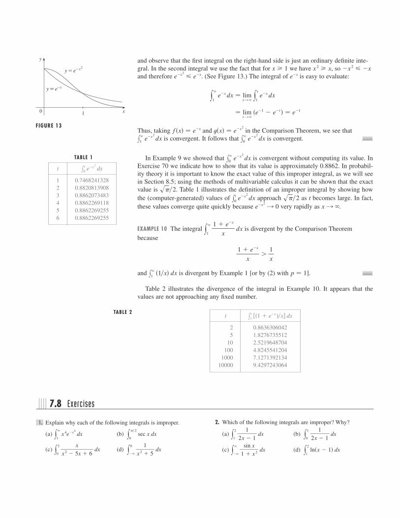
SECTION 7.8 IMPROPER INTEGRALS ❙ ❙ ❙ ❙ 537
and observe that the first integral on the right-hand side is just an ordinary definite inte-gral. In the second integral we use the fact that for we have , so and therefore . (See Figure 13.) The integral of is easy to evaluate:
Thus, taking and in the Comparison Theorem, we see thatis convergent. It follows that is convergent.
In Example 9 we showed that is convergent without computing its value. InExercise 70 we indicate how to show that its value is approximately 0.8862. In probabil-ity theory it is important to know the exact value of this improper integral, as we will seein Section 8.5; using the methods of multivariable calculus it can be shown that the exactvalue is . Table 1 illustrates the definition of an improper integral by showing howthe (computer-generated) values of approach as t becomes large. In fact,these values converge quite quickly because very rapidly as .
EXAMPLE 10 The integral is divergent by the Comparison Theorem
because
and is divergent by Example 1 [or by (2) with ].
Table 2 illustrates the divergence of the integral in Example 10. It appears that the values are not approaching any fixed number.
p � 1x�
1 �1�x� dx
1 � e�x
x�
1
x
y�
1 1 � e�x
x dx
x l �e�x2l 0
s��2xt0 e
�x2 dxs��2
x�
0 e�x2 dx
x�
0 e�x2 dxx�
1 e�x2 dxt�x� � e�x2
f �x� � e�x
� limt l �
�e�1 � e�t � � e�1
y�
1 e�x dx � lim
t l � y
t
1 e�x dx
e�xe�x2 e�x
�x 2 �xx 2 � xx � 1
0
y
x1
y=e_x2
y=e_x
FIGURE 13
TABLE 2t
2 0.86363060425 1.8276735512
10 2.5219648704100 4.8245541204
1000 7.127139213410000 9.4297243064
xt1 ��1 � e�x ��x� dx
TABLE 1
t
1 0.74682413282 0.88208139083 0.88620734834 0.88622691185 0.88622692556 0.8862269255
xt0 e
�x2 dx
2. Which of the following integrals are improper? Why?
(a) (b)
(c) (d) y2
1 ln�x � 1� dxy
�
��
sin x
1 � x 2 dx
y1
0
1
2x � 1 dxy
2
1
1
2x � 1 dx
Explain why each of the following integrals is improper.
(a) (b)
(c) (d) y0
��
1
x 2 � 5 dxy
2
0
x
x 2 � 5x � 6 dx
y��2
0 sec x dxy
�
1 x 4e�x4
dx
1.
|||| 7.8 Exercises

39. 40.
41–46 |||| Sketch the region and find its area (if the area is finite).
41.
42.
;
; 44.
; 45.
; 46.
; 47. (a) If , use your calculator or computer tomake a table of approximate values of for ,5, 10, 100, 1000, and 10,000. Does it appear that is convergent?
(b) Use the Comparison Theorem with to showthat is convergent.
(c) Illustrate part (b) by graphing and on the same screenfor . Use your graph to explain intuitively why
is convergent.
; 48. (a) If , use your calculator or computer tomake a table of approximate values of for ,10, 100, 1000, and 10,000. Does it appear that isconvergent or divergent?
(b) Use the Comparison Theorem with to showthat is divergent.
(c) Illustrate part (b) by graphing and on the same screenfor . Use your graph to explain intuitively why
is divergent.
49–54 |||| Use the Comparison Theorem to determine whether theintegral is convergent or divergent.
49. 50.
52.
53. 54.
55. The integral
is improper for two reasons: The interval is infinite andthe integrand has an infinite discontinuity at 0. Evaluate it byexpressing it as a sum of improper integrals of Type 2 andType 1 as follows:
� y1
0
1
sx �1 � x� dx � y
�
1
1
sx �1 � x� dxy
�
0
1
sx �1 � x� dx
�0, ��
y�
0
1
sx �1 � x� dx
■■ ■■ ■■ ■■ ■■ ■■ ■■ ■■ ■■ ■■ ■■ ■■
y1
0 e�x
sx dxy
� /2
0
dx
x sin x
y�
1
x
s1 � x 6 dxy
�
1
dx
x � e 2x51.
y�
1 2 � e�x
x dxy
�
1
cos2x
1 � x 2 dx
x�
2 t�x� dx2 x 20
tfx
�
2 t�x� dxf �x� � 1�sx
x�
2 t�x� dxt � 5x
t2 t�x� dx
t�x� � 1�(sx � 1)x
�
1 t�x� dx1 x 10
tfx
�
1 t�x� dxf �x� � 1�x 2
x�
1 t�x� dxt � 2x
t1 t�x� dx
t�x� � �sin2x��x 2
■■ ■■ ■■ ■■ ■■ ■■ ■■ ■■ ■■ ■■ ■■ ■■
S � {�x, y� � �2 � x 0, 0 y 1�sx � 2}S � ��x, y� � 0 x � ��2, 0 y sec2x
S � ��x, y� � x � 0, 0 y x��x 2 � 9�
S � ��x, y� � 0 y 2��x 2 � 9�43.
S � ��x, y� � x � �2, 0 y e�x /2
S � ��x, y� � x 1, 0 y e x
■■ ■■ ■■ ■■ ■■ ■■ ■■ ■■ ■■ ■■ ■■ ■■
y1
0 ln x
sx dxy
2
0 z 2 ln z dz
3. Find the area under the curve from to and evaluate it for , , and . Then find the totalarea under this curve for .
; 4. (a) Graph the functions and in theviewing rectangles by and by .
(b) Find the areas under the graphs of and from toand evaluate for , , , , , and .
(c) Find the total area under each curve for , if it exists.
5–40 |||| Determine whether each integral is convergent ordivergent. Evaluate those that are convergent.
5. 6.
8.
9. 10.
11. 12.
14.
15. 16.
17. 18.
19. 20.
22.
23. 24.
25. 26.
28.
29. 30.
32.
33. 34.
35. 36.
37. 38. y2
0
x � 3
2x � 3 dxy
1
�1
e x
e x � 1 dx
y4
0
1
x 2 � x � 6 dxy
�
0 sec x dx
y1
0
1
4y � 1 dyy
33
0 �x � 1��1�5 dx
y1
0
dx
s1 � x 2y3
�2
1
x 4 dx31.
y9
1
1
s3 x � 9
dxy0
�1
1
x 2 dx
y3
0
1
xsx dxy
3
0
1
sx dx27.
y�
0 x arctan x
�1 � x 2�2 dxy�
1 ln x
x 2 dx
y�
1 ln x
x 3 dxy�
��
x 2
9 � x 6 dx
y�
�� e�� x � dxy
�
1 ln x
x dx21.
y6
�� re r�3 dry
�
0 se�5s ds
y�
0
dz
z 2 � 3z � 2y�
1
x � 1
x 2 � 2x dx
y�
0 cos2 dy
�
2� sin � d�
y�
�� x 2e�x3 dxy
�
�� xe�x2 dx13.
y�
�� �2 � v 4� dvy
�
��
x
1 � x 2 dx
y�1
�� e�2 t dty
�
4 e�y�2 dy
y�
0
x
�x 2 � 2�2 dxy�1
��
1
s2 � w dw7.
y0
��
1
2x � 5 dxy
�
1
1
�3x � 1�2 dx
x � 110201010106104100t � 10x � t
x � 1tf�0, 1��0, 100��0, 1��0, 10�
t�x� � 1�x 0.9f �x� � 1�x 1.1
x � 11000100t � 10
x � tx � 1y � 1�x 3
538 ❙ ❙ ❙ ❙ CHAPTER 7 TECHNIQUES OF INTEGRATION

SECTION 7.8 IMPROPER INTEGRALS ❙ ❙ ❙ ❙ 539
56. Evaluate
by the same method as in Exercise 55.
57–59 |||| Find the values of for which the integral converges andevaluate the integral for those values of .
58.
59.
60. (a) Evaluate the integral for , , , and .(b) Guess the value of when is an arbitrary posi-
tive integer.(c) Prove your guess using mathematical induction.
(a) Show that is divergent.(b) Show that
This shows that we can’t define
62. The average speed of molecules in an ideal gas is
where is the molecular weight of the gas, is the gas constant, is the gas temperature, and is the molecularspeed. Show that
63. We know from Example 1 that the regionhas infinite area. Show
that by rotating about the -axis we obtain a solid with finite volume.
64. Use the information and data in Exercises 29 and 30 of Sec-tion 6.4 to find the work required to propel a 1000-kg satelliteout of Earth’s gravitational field.
65. Find the escape velocity that is needed to propel a rocket of mass out of the gravitational field of a planet with mass
and radius . Use Newton’s Law of Gravitation (see Exer-cise 29 in Section 6.4) and the fact that the initial kineticenergy of supplies the needed work.
66. Astronomers use a technique called stellar stereography todetermine the density of stars in a star cluster from theobserved (two-dimensional) density that can be analyzed from
12 mv 2
0
RMm
v0
x�� � ��x, y� � x � 1, 0 y 1�x
v � 8RT
�M
vTRM
v �4
s� � M
2RT�3�2
y�
0 v 3e�Mv2��2RT � dv
y�
�� f �x� dx � lim
t l � y
t
�t f �x� dx
limt l �
yt
�t x dx � 0
x�
�� x dx61.
nx�
0 x ne�x dx321n � 0x
�
0 x ne�x dx
■■ ■■ ■■ ■■ ■■ ■■ ■■ ■■ ■■ ■■ ■■ ■■
y1
0 x p ln x dx
y�
e
1
x �ln x� p dxy1
0
1
x p dx57.
pp
y�
2
1
xsx 2 � 4 dx
a photograph. Suppose that in a spherical cluster of radius the density of stars depends only on the distance from thecenter of the cluster. If the perceived star density is given by
, where is the observed planar distance from the center ofthe cluster, and is the actual density, it can be shown that
If the actual density of stars in a cluster is ,find the perceived density .
67. A manufacturer of lightbulbs wants to produce bulbs that lastabout 700 hours but, of course, some bulbs burn out faster thanothers. Let be the fraction of the company’s bulbs that burnout before hours, so always lies between 0 and 1.(a) Make a rough sketch of what you think the graph of
might look like.(b) What is the meaning of the derivative ?(c) What is the value of ? Why?
68. As we will see in Section 9.4, a radioactive substance decaysexponentially: The mass at time is , where
is the initial mass and is a negative constant. The meanlife of an atom in the substance is
For the radioactive carbon isotope, , used in radiocarbondating, the value of is . Find the mean life of a
atom.
Determine how large the number has to be so that
70. Estimate the numerical value of by writing it asthe sum of and . Approximate the first inte-gral by using Simpson’s Rule with and show that thesecond integral is smaller than , which is less than0.0000001.
71. If is continuous for , the Laplace transform of isthe function defined by
and the domain of is the set consisting of all numbers forwhich the integral converges. Find the Laplace transforms ofthe following functions.(a) (b) (c)
72. Show that if for , where and areconstants, then the Laplace transform exists for .
73. Suppose that and for ,where is continuous. If the Laplace transform of is F�s�f �t�f �
t � 00 f ��t� Ke at0 f �t� Me at
s � aF�s�aMt � 00 f �t� Me at
f �t� � tf �t� � e tf �t� � 1
sF
F�s� � y�
0 f �t�e�st dt
Fft � 0f �t�
x�
4 e�4x dxn � 8
x�
4 e�x2 dxx40 e�x2 dx
x�
0 e�x2 dx
y�
a
1
x 2 � 1 dx � 0.001
a69.
14C�0.000121k
14C
M � �k y�
0 te kt dt
Mkm�0�
m�t� � m�0�e ktt
x�
0 r�t� dtr�t� � F��t�
FF�t�t
F�t�
y�s�x �r� � 1
2 �R � r�2
y�s� � yR
s
2r
sr 2 � s 2 x �r� dr
x �r�sy�s�
rR

540 ❙ ❙ ❙ ❙ CHAPTER 7 TECHNIQUES OF INTEGRATION
5. State the rules for approximating the definite integral with the Midpoint Rule, the Trapezoidal Rule, and Simpson’sRule. Which would you expect to give the best estimate? Howdo you approximate the error for each rule?
6. Define the following improper integrals.
(a) (b) (c)
7. Define the improper integral for each of the follow-ing cases.(a) has an infinite discontinuity at .(b) has an infinite discontinuity at .(c) has an infinite discontinuity at , where .
8. State the Comparison Theorem for improper integrals.
a � c � bcfbfaf
xba f �x� dx
y�
�� f �x� dxy
b
�� f �x� dxy
�
a f �x� dx
xba f �x� dx1. State the rule for integration by parts. In practice, how do you
use it?
2. How do you evaluate if is odd? What if isodd? What if and are both even?
3. If the expression occurs in an integral, what sub-stitution might you try? What if occurs? What if
occurs?
4. What is the form of the partial fraction expansion of a rationalfunction if the degree of is less than the degree of
and has only distinct linear factors? What if a linearfactor is repeated? What if has an irreducible quadraticfactor (not repeated)? What if the quadratic factor is repeated?
Q�x�Q�x�Q
PP�x��Q�x�
sx 2 � a 2
sa 2 � x 2
sa 2 � x 2
nmnmx sinmx cosnx dx
Determine whether the statement is true or false. If it is true, explain why.If it is false, explain why or give an example that disproves the statement.
1. can be put in the form .
2. can be put in the form .
3. can be put in the form .
4. can be put in the form .
5.
6. is convergent.
7. If is continuous, then .x�
�� f �x� dx � lim t l � x t
�t f �x� dxf
y�
1
1
xs2 dx
y4
0
x
x 2 � 1 dx � 1
2 ln 15
A
x�
B
x 2 � 4
x 2 � 4
x �x 2 � 4�
A
x 2 �B
x � 4
x 2 � 4
x 2�x � 4�
A
x�
B
x � 2�
C
x � 2
x 2 � 4
x �x 2 � 4�
A
x � 2�
B
x � 2
x �x 2 � 4�x 2 � 4
8. The Midpoint Rule is always more accurate than theTrapezoidal Rule.
9. (a) Every elementary function has an elementary derivative.(b) Every elementary function has an elementary antiderivative.
10. If is continuous on and is convergent, thenis convergent.
11. If is a continuous, decreasing function on and, then is convergent.
12. If and are both convergent, thenis convergent.
13. If and are both divergent, thenis divergent.
14. If and diverges, then alsodiverges.
x�
0 f �x� dxx�
0 t�x� dxf �x� t�x�
x�
a � f �x� � t�x�� dx
x�
a t�x� dxx�
a f �x� dx
x�
a � f �x� � t�x�� dx
x�
a t�x� dxx�a f �x� dx
x�
1 f �x� dxlimx l � f �x� � 0�1, ��f
x�
0 f �x� dxx
�
1 f �x� dx�0, ��f
77. Find the value of the constant for which the integral
converges. Evaluate the integral for this value of .
78. Find the value of the constant for which the integral
converges. Evaluate the integral for this value of .C
y�
0 � x
x 2 � 1�
C
3x � 1� dx
C
C
y�
0 � 1
sx 2 � 4�
C
x � 2� dx
Cand the Laplace transform of is , show that
74. If is convergent and and are real numbers,show that
75. Show that .
76. Show that by interpreting theintegrals as areas.
x�
0 e�x 2
dx � x10 s�ln y dy
x�
0 x 2e�x 2 dx � 12 x
�
0 e�x 2 dx
ya
�� f �x� dx � y
�
a f �x� dx � y
b
�� f �x� dx � y
�
b f �x� dx
bax�
�� f �x� dx
s � aG�s� � sF�s� � f �0�
G�s�f ��t�
|||| 7 Review■■ C O N C E P T C H E C K ■■
■■ T R U E - F A L S E Q U I Z ■■

39. 40.
41–50 |||| Evaluate the integral or show that it is divergent.
41. 42.
43. 44.
45. 46.
47. 48.
49. 50.
; 51–52 |||| Evaluate the indefinite integral. Illustrate and check thatyour answer is reasonable by graphing both the function and itsantiderivative (take ).
51. 52.
; 53. Graph the function and use the graph toguess the value of the integral . Then evaluate theintegral to confirm your guess.
54. (a) How would you evaluate by hand? (Don’t actually carry out the integration.)
(b) How would you evaluate using tables? (Don’t actually do it.)
(c) Use a CAS to evaluate .(d) Graph the integrand and the indefinite integral on the same
screen.
55–58 |||| Use the Table of Integrals on the Reference Pages to evaluate the integral.
55. 56.
57. 58.
59. Verify Formula 33 in the Table of Integrals (a) by differentia-tion and (b) by using a trigonometric substitution.
60. Verify Formula 62 in the Table of Integrals.
61. Is it possible to find a number such that isconvergent?
x�
0 x n dxn
■■ ■■ ■■ ■■ ■■ ■■ ■■ ■■ ■■ ■■ ■■ ■■
y cot x
s1 � 2 sin x dxy sx 2 � x � 1 dx
y csc5t dty e xs1 � e 2x dx
■■ ■■ ■■ ■■ ■■ ■■ ■■ ■■ ■■ ■■ ■■ ■■
x x 5e�2x dx
x x 5e�2x dx
x x 5e�2x dxCAS
x2�
0 f �x� dxf �x� � cos2x sin3x
■■ ■■ ■■ ■■ ■■ ■■ ■■ ■■ ■■ ■■ ■■ ■■
y x 3
sx 2 � 1 dxy ln�x 2 � 2x � 2� dx
C � 0
■■ ■■ ■■ ■■ ■■ ■■ ■■ ■■ ■■ ■■ ■■ ■■
y�
1 tan�1x
x 2 dxy�
��
dx
4x 2 � 4x � 5
y1
�1 x � 1
s3 x 4
dxy3
0
dx
x 2 � x � 2
y1
0
1
2 � 3x dxy
4
0 ln x
sx dx
y6
2
y
sy � 2 dyy
�
2
dx
x ln x
y1
0 t 2 � 1
t 2 � 1 dty
�
1
1
�2x � 1�3 dx
■■ ■■ ■■ ■■ ■■ ■■ ■■ ■■ ■■ ■■ ■■ ■■
y��3
��4 stan �
sin 2� d�y
1�2
0
xe 2x
�1 � 2x�2 dxNote: Additional practice in techniques of integration is provided inExercises 7.5.
1–40 |||| Evaluate the integral.
1. 2.
3. 4.
5. 6.
7. 8.
9. 10.
11. 12.
13. 14.
15. 16.
17. 18.
19. 20.
21. 22.
23. 24.
25. 26.
27. 28.
29. 30.
31. 32.
33. 34.
35. 36.
37. 38. y x �tan�1x�2 dxy �cos x � sin x�2 cos 2x dx
y 1 � tan �
1 � tan � d�y
1
sx � x 3�2 dx
y �arcsin x�2 dxy x 2
�4 � x 2 �3�2 dx
y��4
0 x sin x
cos3x dxy
ln 10
0 e x
se x � 1
e x � 8 dx
y dx
e xs1 � e�2xy
1
�1 x 5 sec x dx
y s3 x � 1
s3 x � 1
dxy��2
0 cos3x sin 2x dx
y dx
1 � e xy 3x 3 � x 2 � 6x � 4
�x 2 � 1��x 2 � 2� dx
y e x cos x dxy csc4 4x dx
y x 3
�x � 1�10 dxy dx
sx 2 � 4x
y dt
sin2t � cos 2ty x � 1
9x 2 � 6x � 5 dx
y x 2 � 8x � 3
x 3 � 3x 2 dxy x sec x tan x dx
y sec6�
tan2� d�y sin2� cos5� d�
y x 2 � 2
x � 2 dxy
dx
x 3 � x
y1
�1
sin x
1 � x 2 dxy2
1 sx 2 � 1
x dx
y1
0 sarctan x
1 � x 2 dxy4
1 x 3�2 ln x dx
y dx
x 2s1 � x 2y
sin�ln t�t
dt
y 1
y 2 � 4y � 12 dyy tan7x sec3x dx
y4
1
dt
�2t � 1�3y��2
0
cos �
1 � sin � d�
y5
0 ye�0.6y dyy
5
0
x
x � 10 dx
CHAPTER 7 REVIEW ❙ ❙ ❙ ❙ 541
■■ E X E R C I S E S ■■

point to be 53 cm. The circumference 7 cm from each end is45 cm. Use Simpson’s Rule to make your estimate.
71. Use the Comparison Theorem to determine whether the integral
is convergent or divergent.
72. Find the area of the region bounded by the hyperbolaand the line .
73. Find the area bounded by the curves and between and .
74. Find the area of the region bounded by the curves, , and .
75. The region under the curve , is rotatedabout the -axis. Find the volume of the resulting solid.
76. The region in Exercise 75 is rotated about the -axis. Find thevolume of the resulting solid.
77. If is continuous on and , show that
78. We can extend our definition of average value of a continuousfunction to an infinite interval by defining the average value of
on the interval to be
(a) Find the average value of on the interval .(b) If and is divergent, show that the aver-
age value of on the interval is , if thislimit exists.
(c) If is convergent, what is the average value of on the interval ?
(d) Find the average value of on the interval .
79. Use the substitution to show that
80. The magnitude of the repulsive force between two point chargeswith the same sign, one of size 1 and the other of size , is
where is the distance between the charges and is aconstant. The potential at a point due to the charge isdefined to be the work expended in bringing a unit charge to from infinity along the straight line that joins and . Find aformula for .V
PqP
qPV 0r
F �q
4� 0r 2
q
y�
0
ln x
1 � x 2 dx � 0
u � 1�x
�0, ��y � sin x�a, ��
fx�
a f �x� dx
lim x l � f �x��a, ��fx
�
a f �x� dxf �x� � 0�0, ��y � tan�1x
lim t l �
1
t � a y
t
a f �x� dx
�a, ��f
y�
0 f ��x� dx � �f �0�
lim x l � f �x� � 0�0, ��f �
y
xy � cos2x, 0 x ��2
x � 1y � 1�(2 � sx )y � 1�(2 � sx )
x � �x � 0y � cos2xy � cos x
y � 3y 2 � x 2 � 1
y�
1
x 3
x 5 � 2 dx
28 cm
62. For what values of is convergent? Evaluate theintegral for those values of .
63–64 |||| Use (a) the Trapezoidal Rule, (b) the Midpoint Rule, and(c) Simpson’s Rule with to approximate the given integral.Round your answers to six decimal places.
63. 64.
65. Estimate the errors involved in Exercise 63, parts (a) and (b).How large should be in each case to guarantee an error ofless than 0.00001?
66. Use Simpson’s Rule with to estimate the area under thecurve from to .
67. The speedometer reading ( ) on a car was observed at 1-minute intervals and recorded in the chart. Use Simpson’sRule to estimate the distance traveled by the car.
68. A population of honeybees increased at a rate of bees perweek, where the graph of is as shown. Use Simpson’s Rulewith six subintervals to estimate the increase in the bee popula-tion during the first 24 weeks.
69. (a) If , use a graph to find an upper bound for .
(b) Use Simpson’s Rule with to approximate and use part (a) to estimate the error.
(c) How large should be to guarantee that the size of theerror in using is less than ?
70. Suppose you are asked to estimate the volume of a football.You measure and find that a football is 28 cm long. You use apiece of string and measure the circumference at its widest
0.00001Sn
nx
�
0 f �x� dxn � 10
� f �4��x��f �x� � sin�sin x�CAS
r
0 2420161284(weeks)
t
4000
8000
12000
rr�t�
v
x � 4x � 1y � e x�xn � 6
n
■■ ■■ ■■ ■■ ■■ ■■ ■■ ■■ ■■ ■■ ■■ ■■
y��2
0 ssin x dxy
1
0 s1 � x 4 dx
n � 10
ax
�
0 e ax cos x dxa
542 ❙ ❙ ❙ ❙ CHAPTER 7 TECHNIQUES OF INTEGRATION
t (min) (mi�h) t (min) (mi�h)
0 40 6 561 42 7 572 45 8 573 49 9 554 52 10 565 54
vv

Cover up the solution to the example and try it yourself first.
EXAMPLE(a) Prove that if is a continuous function, then
(b) Use part (a) to show that
for all positive numbers .
SOLUTION(a) At first sight, the given equation may appear somewhat baffling. How is it possibleto connect the left side to the right side? Connections can often be made through one ofthe principles of problem solving: introduce something extra. Here the extra ingredient isa new variable. We often think of introducing a new variable when we use the Substitu-tion Rule to integrate a specific function. But that technique is still useful in the presentcircumstance in which we have a general function .
Once we think of making a substitution, the form of the right side suggests that itshould be . Then . When , ; when , . So
But this integral on the right side is just another way of writing . So the givenequation is proved.
(b) If we let the given integral be and apply part (a) with , we get
A well-known trigonometric identity tells us that and, so we get
Notice that the two expressions for are very similar. In fact, the integrands have thesame denominator. This suggests that we should add the two expressions. If we do so,we get
Therefore, .I � ��4
2I � y��2
0 sinnx � cosnx
sinnx � cosnx dx � y
��2
0 1 dx �
�
2
I
I � y��2
0
cosnx
cosnx � sinnx dx
cos���2 � x� � sin xsin���2 � x� � cos x
I � y��2
0
sinnx
sinnx � cosnx dx � y
��2
0
sinn���2 � x�sinn���2 � x� � cosn���2 � x�
dx
a � ��2I
xa0 f �x� dx
ya
0 f �a � x� dx � �y
0
a f �u� du � y
a
0 f �u� du
u � 0x � au � ax � 0du � �dxu � a � x
f
n
y��2
0
sinnx
sinnx � cosnx dx �
�
4
ya
0 f �x� dx � y
a
0 f �a � x� dx
f
PROBLEMS PLUS
|||| The principles of problem solving arediscussed on page 80.
|||| The computer graphs in Figure 1 make itseem plausible that all of the integrals in theexample have the same value. The graph of eachintegrand is labeled with the correspondingvalue of .n
1
0
1243
π2
FIGURE 1

; 1. Three mathematics students have ordered a 14-inch pizza. Instead of slicing it in the tradi-tional way, they decide to slice it by parallel cuts, as shown in the figure. Being mathematicsmajors, they are able to determine where to slice so that each gets the same amount of pizza.Where are the cuts made?
2. Evaluate .
The straightforward approach would be to start with partial fractions, but that would be brutal.Try a substitution.
3. Evaluate .
4. A man initially standing at the point walks along a pier pulling a rowboat by a rope oflength . The man keeps the rope straight and taut. The path followed by the boat is a curvecalled a tractrix and it has the property that the rope is always tangent to the curve (see thefigure). (a) Show that if the path followed by the boat is the graph of the function , then
(b) Determine the function .
5. A function is defined by
Find the minimum value of .
6. If is a positive integer, prove that
7. Show that
Hint: Start by showing that if denotes the integral, then
; 8. Suppose that is a positive function such that is continuous. (a) How is the graph of related to the graph of ? What happens
as ?(b) Make a guess as to the value of the limit
based on graphs of the integrand.(c) Using integration by parts, confirm the guess that you made in part (b). [Use the fact that,
since is continuous, there is a constant such that for .]
9. If , find .limt l 0
�y1
0 �bx � a�1 � x�� t dx�1�t
0 � a � b
0 � x � 1 f ��x� � MMf �
lim n l �
y1
0 f �x� sin nx dx
n l �y � f �x�y � f �x� sin nx
f �f
Ik�1 �2k � 2
2k � 3 Ik
In
y1
0 �1 � x 2 �n dx �
22n�n!�2
�2n � 1�!
y1
0 �ln x�n dx � ��1�n n!
n
f
0 � x � 2�f �x� � y�
0 cos t cos�x � t� dt
f
y � f �x�
f ��x� �dy
dx�
�sL 2 � x 2
x
y � f �x�
LO
y1
0 (s3 1 � x7 � s
7 1 � x 3) dx
y 1
x 7 � x dx
PROBLEMS
y
xO
(L, 0)
(x, y)Lpier
FIGURE FOR PROBLEM 4
FIGURE FOR PROBLEM 1
14 in

; 10. Graph and use the graph to estimate the value of such that is amaximum. Then find the exact value of that maximizes this integral.
11. The circle with radius 1 shown in the figure touches the curve twice. Find the areaof the region that lies between the two curves.
12. A rocket is fired straight up, burning fuel at the constant rate of kilograms per second. Letbe the velocity of the rocket at time and suppose that the velocity of the exhaust
gas is constant. Let be the mass of the rocket at time and note that decreasesas the fuel burns. If we neglect air resistance, it follows from Newton’s Second Law that
where the force . Thus
Let be the mass of the rocket without fuel, the initial mass of the fuel, and. Then, until the fuel runs out at time , the mass is .
(a) Substitute into Equation 1 and solve the resulting equation for . Use theinitial condition to evaluate the constant.
(b) Determine the velocity of the rocket at time . This is called the burnout velocity.(c) Determine the height of the rocket at the burnout time.(d) Find the height of the rocket at any time .
13. Use integration by parts to show that, for all ,
; 14. The Chebyshev polynomials are defined by
, , , , . . .
(a) What are the domain and range of these functions?(b) We know that and . Express explicitly as a quadratic polynomial
and as a cubic polynomial.(c) Show that, for ,
(d) Use part (c) to show that is a polynomial of degree .(e) Use parts (b) and (c) to express and explicitly as polynomials.(f) What are the zeros of ? At what numbers does have local maximum and minimum
values?(g) Graph , , , and on a common screen.(h) Graph , , and on a common screen.(i) Based on your observations from parts (g) and (h), how are the zeros of related to the
zeros of ? What about the -coordinates of the maximum and minimum values?(j) Based on your graphs in parts (g) and (h), what can you say about when is
odd and when is even?(k) Use the substitution to evaluate the integral in part ( j).(l) The family of functions are defined even when is not an integer
(but then is not a polynomial). Describe how the graph of changes as increases.cffcf �x� � cos�c arccos x�
u � arccos xn
nx1�1 Tn�x� dx
xTn�1
Tn
T7T6T5
T5T4T3T2
TnTn
T7T5, T6,T4,nTn
Tn�1�x� � 2xTn�x� � Tn�1�x�
n 1T3
T2T1�x� � xT0�x� � 1
321n � 0Tn�x� � cos�n arccos x�
Tn
0 � y�
0
sin t
ln�1 � x � t� dt �
2
ln�1 � x�
x 0
ty � y�t�
t � M2�bv�0� � 0
vM � M0 � btM � M0 � btt � M2bM0 � M1 � M2
M2M1
M dv
dt� ub � �Mt1
F � �Mt
F � M dv
dt� ub
MtM � M�t�utv � v�t�
b
y � 2x t
xt�1t f �x� dxtf �x� � sin�e x �
FIGURE FOR PROBLEM 11
y=| 2x |
y
0 x