TECHNICAL REPORT

MODAL ANALYSIS USING THE SINGULAR VALUE DECOMPOSITION AND RATIONAL FRACTION POLYNOMIALS

By

J. B. Fahnline, R. L. Campbell, S. A. Hambric, and M. R. Shepherd

DISTRIBUTION STATEMENT A: Approved for public release. Distribution is unlimited.

The Pennsylvania State University The Applied Research Laboratory

P. O. Box 30 State College, PA 16804

Modal Analysis Using the Singular Value Decomposition and Rational Fraction Polynomials

By

J. B. Fahnline, R. L. Campbell, S. A. Hambric, and M. R. Shepherd

Technical Report TR 17-005 6 April 2017

Supported by: Paul E. Sullivan, Director Applied Research Laboratory

DISTRIBUTION STATEMENT A: Approved for public release. Distribution is unlimited.

Standard Form 298 (Rev. 8/98)

REPORT DOCUMENTATION PAGE

Prescribed by ANSI Std. Z39.18

Form Approved OMB No. 0704-0188

The public reporting burden for this collection of information is estimated to average 1 hour per response, including the time for reviewing instructions, searching existing data sources, gathering and maintaining the data needed, and completing and reviewing the collection of information. Send comments regarding this burden estimate or any other aspect of this collection of information, including suggestions for reducing the burden, to Department of Defense, Washington Headquarters Services, Directorate for Information Operations and Reports (0704-0188), 1215 Jefferson Davis Highway, Suite 1204, Arlington, VA 22202-4302. Respondents should be aware that notwithstanding any other provision of law, no person shall be subject to any penalty for failing to comply with a collection of information if it does not display a currently valid OMB control number. PLEASE DO NOT RETURN YOUR FORM TO THE ABOVE ADDRESS. 1. REPORT DATE (DD-MM-YYYY) 2. REPORT TYPE 3. DATES COVERED (From - To)

4. TITLE AND SUBTITLE 5a. CONTRACT NUMBER

5b. GRANT NUMBER

5c. PROGRAM ELEMENT NUMBER

5d. PROJECT NUMBER

5e. TASK NUMBER

5f. WORK UNIT NUMBER

6. AUTHOR(S)

7. PERFORMING ORGANIZATION NAME(S) AND ADDRESS(ES) 8. PERFORMING ORGANIZATION REPORT NUMBER

9. SPONSORING/MONITORING AGENCY NAME(S) AND ADDRESS(ES) 10. SPONSOR/MONITOR'S ACRONYM(S)

11. SPONSOR/MONITOR'S REPORT NUMBER(S)

12. DISTRIBUTION/AVAILABILITY STATEMENT

13. SUPPLEMENTARY NOTES

14. ABSTRACT

15. SUBJECT TERMS

16. SECURITY CLASSIFICATION OF: a. REPORT b. ABSTRACT c. THIS PAGE

17. LIMITATION OF ABSTRACT

18. NUMBER OF PAGES

19a. NAME OF RESPONSIBLE PERSON

19b. TELEPHONE NUMBER (Include area code)

08-04-2017 Technical Report October 2004 - April 2017

Modal Analysis Using the Singular Value Decomposition and RationalFraction Polynomials

J. B. Fahnline, R. L. Campbell, S. A. Hambric, and M. R. Shepherd

Applied Research LaboratoryPO Box 30State College, PA 16804

TR 17-005

Applied Research LaboratoryPO Box 30State College, PA 16804

ARL Penn State

TR 17-005

Distribution Statement A: Approved for public release. Distribution is unlimited.

This report documents the computer codes developed at the Penn State Applied Research Laboratory to extract modal informationfrom experimental vibration measurements. It includes discussions of the numerical techniques used in the analysis, formats for theinput files, output from the computer codes, and interpretation of the results. The programs are designed for experimental datasetswith multiple drive and response points and have proven effective even for systems with numerous closely-spaced resonancefrequencies and relatively high noise levels. For the final stage of the analysis, a graphical interface has been developed to simplifythe process of eliminating misidentified modes and refining the predictions for the resonance frequencies, loss factors, and modeshapes. An example problem of a pipe with a bend is used to illustrate the required input and the expected results. Measurements ofmultiple input-multiple output data for experimental modal analysis can also be useful for computing quantities relevant to statisticalenergy analysis, and thus calculations for power injection and radiation loss factors are also documented.

Singular value decomposition, rational fraction polynomial, SVD, RFP, modal analysis, loss factor

U U U UU 53

Robert L. Campbell

814-865-1741

1

Abstract This report documents the computer codes developed at the Penn State Applied Research Laboratory to extract modal information from experimental vibration measurements. It includes discussions of the numerical techniques used in the analysis, formats for the input files, output from the computer codes, and interpretation of the results. The programs are designed for experimental datasets with multiple drive and response points and have proven effective even for systems with numerous closely-spaced resonance frequencies and relatively high noise levels. For the final stage of the analysis, a graphical interface has been developed to simplify the process of eliminating misidentified modes and refining the predictions for the resonance frequencies, loss factors, and mode shapes. An example problem of a pipe with a bend is used to illustrate the required input and the expected results. Measurements of multiple input-multiple output data for experimental modal analysis can also be useful for computing quantities relevant to statistical energy analysis, and thus calculations for power injection and radiation loss factors are also documented.

2

Table of Contents Abstract ............................................................................................................................................... 1 

List of Figures ..................................................................................................................................... 3 

INTRODUCTION .............................................................................................................................. 4 

A. The Basic Analysis Steps .............................................................................................................. 5 

B. Discrete Fourier Series Decomposition ......................................................................................... 8 

C. Application of the Singular Value Decomposition ..................................................................... 12 

D. Finding the Resonances .............................................................................................................. 14 

E. Modal Parameter Identification ................................................................................................... 20 

F. Mass Normalization within MODAL_ANALYSIS_USING_SVD ............................................... 21 

G. Eliminating Misidentified Resonance Peaks and Refining the Predictions ................................ 23 

H. Computing Mode Shapes using the Output from the RFP Analysis ........................................... 29 

I. Energy, Conductance, and Loss Factors for Statistical Energy Analysis ..................................... 37 

J. Summary and Future Work ........................................................................................................... 39 

REFERENCES ................................................................................................................................. 40 

APPENDIX A: Input File Formats ................................................................................................... 42 

APPENDIX B: Step-By-Step Instructions for Modal Analysis ....................................................... 44 

APPENDIX C: Description of Output Files from the Computer Codes .......................................... 46 

APPENDIX D: One-third-octave Power Estimation ........................................................................ 52 

3

List of Figures

Figure 1. Picture of a pipe with a bend instrumented for a modal test and the accompanying surface mesh. ................................................................................................................................ 9 

Figure 2. Discrete Fourier series decomposition of the vibrations of one ring of elements around the pipe. ............................................................................................................................... 11 

Figure 3. Mode shapes for resonances clustered near the cut-on frequency for N = 3 modes. ....... 12 

Figure 4. Singular values for the pipe with a bend as a function of frequency. .............................. 13 

Figure 5. Modal transfer functions (solid lines) overlaid on the singular values for the pipe with a bend. ............................................................................................................................... 14 

Figure 6. “Snapshot” of the graphical interface for the MATLAB program siftSVD with a unit fit order. .............................................................................................................................. 15 

Figure 7. Input to, and output from, the Savitz-Golay smoothing filter. ......................................... 17 

Figure 8. Original circle fit and circle fit after rotating it and making it pass through the origin. .. 19 

Figure 9. Measured and synthesized drive point acceleration-to-force transfer functions from MODAL_ANALYSIS_USING_SVD. ............................................................................. 23 

Figure 10. “Snapshot” of the graphical interface for the MATLAB program siftSVD with a fit order of 1. ................................................................................................................................ 24 

Figure 11. Singular values as a function of frequency showing “scalloping”. ................................ 26 

Figure 12. Singular values as a function of frequency showing “scalloping”. ................................ 26 

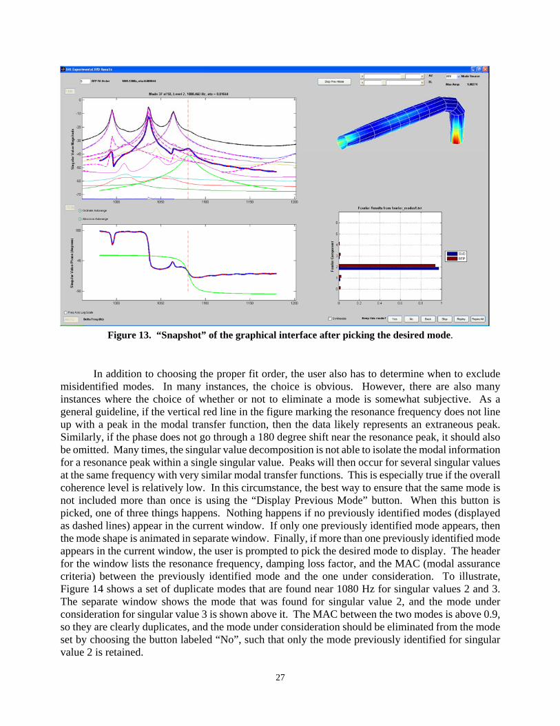
Figure 13. “Snapshot” of the graphical interface after picking the desired mode. .......................... 27 

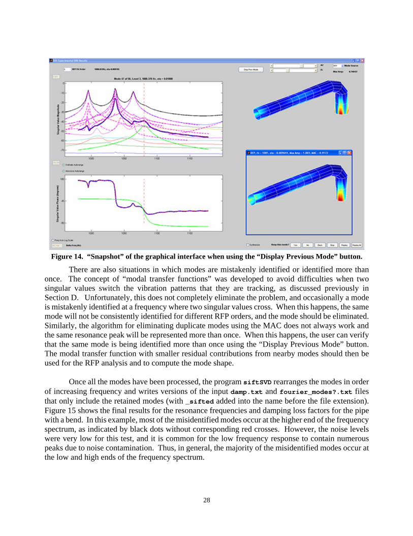
Figure 14. “Snapshot” of the graphical interface when using the “Display Previous Mode” button. ....................................................................................................................................... 28 

Figure 15. Predicted loss factors for the pipe with a bend. .............................................................. 29 

Figure 16. Transfer function amplitude as a function of frequency for various nodal locations. .... 34 

Figure 17. Mode shapes derived from the SVD (left) and the least squares procedure using the RFP modal parameter information (right). ............................................................................ 35 

Figure 18. Mode shapes derived from the SVD (left) and the least squares procedure using the RFP modal parameter information (right). ............................................................................ 36 

Figure 19. Measured and synthesized drive point transfer functions from siftSVD for SVD mode shapes. ............................................................................................................................ 36 

Figure 20. Measured and synthesized drive point transfer functions from siftSVD for RFP mode shapes. ............................................................................................................................ 37 

4

INTRODUCTION This report documents the computer codes developed at Penn State University’s Applied Research Laboratory to extract modal information from experimental vibration measurements. The programs were developed to improve upon, and replace, existing commercial modal analysis software packages that had been used in the past to process modal analysis data. The codes were developed from a user’s viewpoint, such that much of the effort has been devoted to refining the predictions or simplifying the process of performing an experimental modal analysis. The numerical techniques used to analyze the data were chosen primarily because they worked well for practical problems of interest and could be easily incorporated into the computer codes. Thus, little effort has been devoted to developing new numerical techniques unless an existing technique was in some way inadequate. Overall, the computer codes lack some of the refinements of commercial software packages, but can be easily adapted or refined to address future problems of interest. This report is also written from a user’s viewpoint, with the main emphasis on providing enough detailed information to understand the numerical techniques implemented in the computer programs. Not much effort is devoted to comparing and contrasting competing methods or to providing background material available elsewhere. For the novice user, thorough overviews of experimental modal analysis can be found in the books by Ewins [1], Maia, et al. [2] and the review papers by Allemang and Brown [3] and Formenti and Richardson [4]. The proceedings of the Experimental Modal Analysis Conference provide a good survey of the current state-of-the-art, which is rapidly evolving due to a proliferation of research in both the commercial and academic sectors. This is especially true of techniques for processing multiple-input, multiple-output (MIMO) datasets, which are the main focus of the computer programs documented here. The complex mode indicator function (CMIF) technique developed at the University of Cincinnati forms the basis of the ARL modal analysis program. It relies heavily on the singular value decomposition (SVD) to help separate the modes before the modal identification process begins [5-8]. In a typical calculation, the modal analysis data for a single frequency is arranged in matrix form with each column representing the response to a different drive point and each row representing a different response point. The matrix is input to the singular value decomposition algorithm and left- and right-singular vectors and a diagonal singular value matrix are computed. The calculation is repeated at each analysis frequency and the resulting data is used to identify the modal parameters. In the optimal situation, the singular value decomposition will completely separate the modes from each other, so that a single transfer function is produced for each mode with no residual effects. In practice, the modal transfer functions are never completely free from residual effects of nearby modes, and a secondary analysis is required to properly identify the modal parameters. Fortunately, MATLAB includes a number of fairly sophisticated nonlinear least square fitting routines that can be used to perform a standard rational fraction polynomial fit to the data and remove residual effects. The implementation within ARL’s modal analysis software follows the same basic steps as the original CMIF technique, but many of the details are different. Significant effort has been devoted to (1) automatically identifying modes, especially in the presence of high noise levels, (2) developing a graphical user interface to help simplify the process of eliminating misidentified modes, and (3) developing additional techniques to help further describe the modal content, such as a discrete Fourier series decomposition. In general, the process is very successful and relatively efficient as long as the

5

input data is of high quality and has adequate spatial resolution to discriminate between the modes. Also, the results are better if the drive point locations are chosen to ensure that, as much as possible, they are not at nodal lines for the modes. If the data does not meet these requirements, it is unlikely that any modal analysis algorithm will be successful. Much of the onus is thus placed on the user to define and measure the surface vibrations with adequate resolution.

A. The Basic Analysis Steps Before going into details, a brief description of the general analysis flow will be given. The optional steps are performed if mode shapes are to be computed as well as resonance frequencies and loss factors. The analysis begins with measurements of the vibrational response of a structure either due to a known input force. For example, accelerometers can be used to measure the vibrational response of a structure due to an impact with a force hammer. Until recently, experimental modal analysis was typically performed by measuring acceleration-to-force transfer functions with a single accelerometer and multiple hit locations. It is now more common to employ multiple accelerometers and hit point locations, yielding MIMO data. A guide to proper techniques for this type of measurement can be found in the class notes by Allemang [9]. Typically, both the drive and response points are “numbered” during the data acquisition process and these locations are translated into a surface element mesh. It is important for the drive and response points to be numbered consistently so that the programs can identify locations with coincident drive and response points. In the present implementation, measurements in different directions at the same location are given different numbers so that the mode shapes can be animated properly. The second step is to convert the vibration or transfer function data to universal file format (UFF) for Universal Dataset Number 58. This format is preferred because it is relatively compact and can easily be read and edited using a text editor. The basic specifications for the UFF can be found on the web at http://www.sdrl.uc.edu/uff2/uff2.html and an excerpt from a sample UFF file is given in Appendix A. An internal, binary data format is also recognized. Each transfer function contains information for the drive and response point numbers and directions, the number of frequencies, the frequency increment, and, of course, the actual complex-valued transfer function or acceleration data. Because the file format is only designed for input directions along the x-, y-, or z-axis, the directions listed in the UFF files are ignored by the software, and the surface element mesh is used to compute the direction normal to the surface. For Data Physics files, the MATLAB program dp2uff (Y:\Common\Noise Control and Acoustic Division\Structural Acoustics

Department\Matlab\FE_BETools) can be used to create a UFF text file. Files from LabVIEW can be converted by running the program importFreqData (formerly LVimpact2UFF, see Y:\Common\Noise Control and Acoustic Division\Structural Acoustics

Department\LabVIEW). The resulting file should be named exp_data.txt or exp_data.bin. The next step, which is optional, is to generate coherence data as a function of frequency between each of the input and output channels. This is not necessary when the overall coherence is high, but difficulties can occur in the modal parameter identification routines if transfer functions with low coherence are included, especially if the resulting data has much higher amplitude than the actual transfer function data. This is typically a problem for underwater measurements, where some of the accelerometers will work intermittently, depending on the length of time they are submerged.

6

The coherence data is written by the program LVimpact2UFF in the same format as the transfer function data in the file exp_data.txt with the name exp_data_coh.txt. A secondary program named FIND_BAD_DATA is used to average the coherence data over the whole frequency range and write a file named xfer_function_coh_ave.txt containing the average coherence for each transfer function. If this file is present in the working directory, any transfer function data with average coherence less than 0.7 is set to zero before the singular value decomposition is computed. The fourth step, which is also an optional step but necessary for outputting mode shapes, is to generate a geometry file representing the surface locations for the transfer function or vibration data. It should be in the standard format for input files to the boundary element program POWER and should be named geom.txt. An excerpt from a sample geom.txt file is given in Appendix A. Typically, the mesh is created using a finite element preprocessing program, such as FEMAP, or it can be generated manually. The text editor VI is useful for editing the FEMAP output files to make them conform to the specified file format. The node ordering for elements of the mesh should be consistent, so that the normal directions are also consistent. In the subsequent analysis, the normal direction at each node is computed using the cross product of the connected element edges, and then the normal directions are averaged over all the elements connected to the node. It is sometimes useful to have multiple nodes at the same location so that the normal directions are computed appropriately for the individual nodes. If the mode shapes are intended primarily to help in identifying the modes, the nodal locations do not have to be input precisely. However, if experimental vibration data is to be input to the program FORCE to compute radiated noise, the nodal locations should be input with care to enable accurate calculations of surface normal velocities. It is also possible to spatially decompose the vibration data using a discrete Fourier transform for subsets of the surface element mesh. If this is desired, the geometry files for the element subsets should be generated and given the name(s) geom_fourier1.txt, geom_fourier2.txt, etc. A thorough discussion of the Fourier decomposition technique is given in the next section.

The fifth step, which is optional but recommended, is to generate an in.txt file containing

input values for the parameters. An excerpt from a sample in.txt file is given in Appendix A. For experimental modal analyses, the main inputs are:

(1) CV – the factor to convert the nodal locations to meters, (2) NP – the number of singular values to search for peaks, (3) PP – the output format for the data (should be set to 3 to output the mode shapes), (4) NG – determines whether or not modes with negative damping are included in the

output ( 0 = No, 1 = Yes ), (5) SW – determines whether or not the number of drive points is greater than the number

of response points ( 0 = No, 1 = Yes ), and (6) NF – the number of frequencies to output for the RFP analysis in siftSVD (default =

128). More detailed discussions of the parameters are given subsequently when they are relevant to the analysis. Although it is good practice to apply the sensitivities during the data acquisition and conversion process, it is sometimes necessary to apply a gain subsequently using the input parameter GN. The in.txt file can also be used to choose the level of rotational symmetry for the discrete Fourier transform calculations using the parameter GF, requiring a separate line for each geometry file. If an in.txt file is not present in the directory where the exp_data file resides, the program

7

assumes the geom.txt file is in meters, the gain is unity, and all but the smallest singular value is searched for resonance peaks.

Once all the input files have been generated, the program MODAL_ANALYSIS_USING_SVD is

run to extract the modal parameters. The source code is written in FORTRAN 90, and the executable file is created using the MICROSOFT VISUAL STUDIO environment for WINDOWS. It should be possible to recompile the program for other environments and platforms. To reduce the text file sizes, the program converts the experimental data to binary and stores it in a file named exp_data.bin. This step is ignored if the file is already in binary format. The accompanying NODE_list_drive.txt, NODE_list_response.txt, and FREQ_list.txt files supply the rest of the information contained in the original exp_data.txt file. As discussed subsequently, the program MODAL_ANALYSIS_USING_SVD is designed to automatically identify the resonance peaks from the output of the singular value decomposition. In an effort to prevent modes from being excluded, the tolerances in the mode detection algorithm have been set fairly loosely, such that a number of extraneous modes are inevitably identified. If the data are “noisy”, it is possible for the number of peaks identified to exceed the number of analysis frequencies, causing an array to become “out-of-bounds” . To correct the problem and allow the program to run to completion, the parameter NP in the in.txt file can be reduced such that fewer singular values are searched for resonance peaks during the process of automatically identifying the modes. After running MODAL_ANALYSIS_USING_SVD, the MATLAB program siftSVD is run to eliminate misidentified peaks and to refine the predictions for the resonance frequencies and damping loss factors. To help simplify the process, each modal transfer function is plotted, one at a time, overlaid on a plot of the singular values. Also, a secondary plot shows the phase for the modal transfer function. The user is then prompted to choose, yes or no, if the mode should be retained. Admittedly, this process can be tedious for structures with numerous modes or high noise levels and the choice of whether or not to keep a specific mode can be somewhat subjective. However, it is preferable to the industry practice of selecting a frequency band of interest and inputting the number of modes within the band. As part of the calculation, the resonance frequencies and damping loss factor predictions are refined using rational fraction polynomials. Typically, the rational fraction polynomial does a better job of isolating the data for a single mode, and yields slightly lower loss factors. The differences become appreciable only if the spatial resolution of the surface mesh is inadequate or if the mode is not excited to a high level of vibration, which is a function of the drive point locations. After performing an analysis with the full dataset, it is sometimes useful to remove transfer function data for some of the drive or response points, and/or reduce the frequency range or the frequency spacing. For example, if an accelerometer did not work at all during the measurements, it is best to remove it completely from the analysis. This can be accomplished using the program REMOVE_DRIVE_POINTS_RESPONSE_POINTS_AND_OR_FREQUENCIES. To use the program, the user creates files named NODE_list_drive_reduced.txt, and NODE_list_response_reduced.txt, with 0’s replacing the node numbers for the channels that are to be eliminated. If only the number of analysis frequencies is to be reduced, the original files can simply be copied directly to the new file name. The program will write out drive and response point lists without the zeros named NODE_list_drive_reduced_wo_zeros.txt, and NODE_list_response_reduced_wo_zeros.txt, respectively. When the program is run, it will ask the user to input the lower and upper frequencies

8

for the reduced dataset and the number of frequencies to skip after each one that is kept. A file named FREQ_list_reduced.txt is written containing the analysis frequencies for the reduced dataset. Reducing the analysis frequency range or spacing can be useful in a number of circumstances. For example, the frequency resolution is chosen to resolve low frequency modes with low damping, but for simplicity, a single measurement is used to capture the full range of interest. At the upper end of the frequency range, the damping tends to be much higher and the modal overlap is higher, such that the peaks become overly resolved. This makes it difficult to identify peaks because the transfer function data does not change significantly over the frequency range used to identify the modes. Reducing the frequency spacing then makes it much easier to identify resonances and also reduces the analysis times. (However, it is unrealistic to expect reducing the frequency spacing to allow numerous new modes to be identified when the modal overlap is high because there are typically too few accelerometers to discriminate between the modes.)

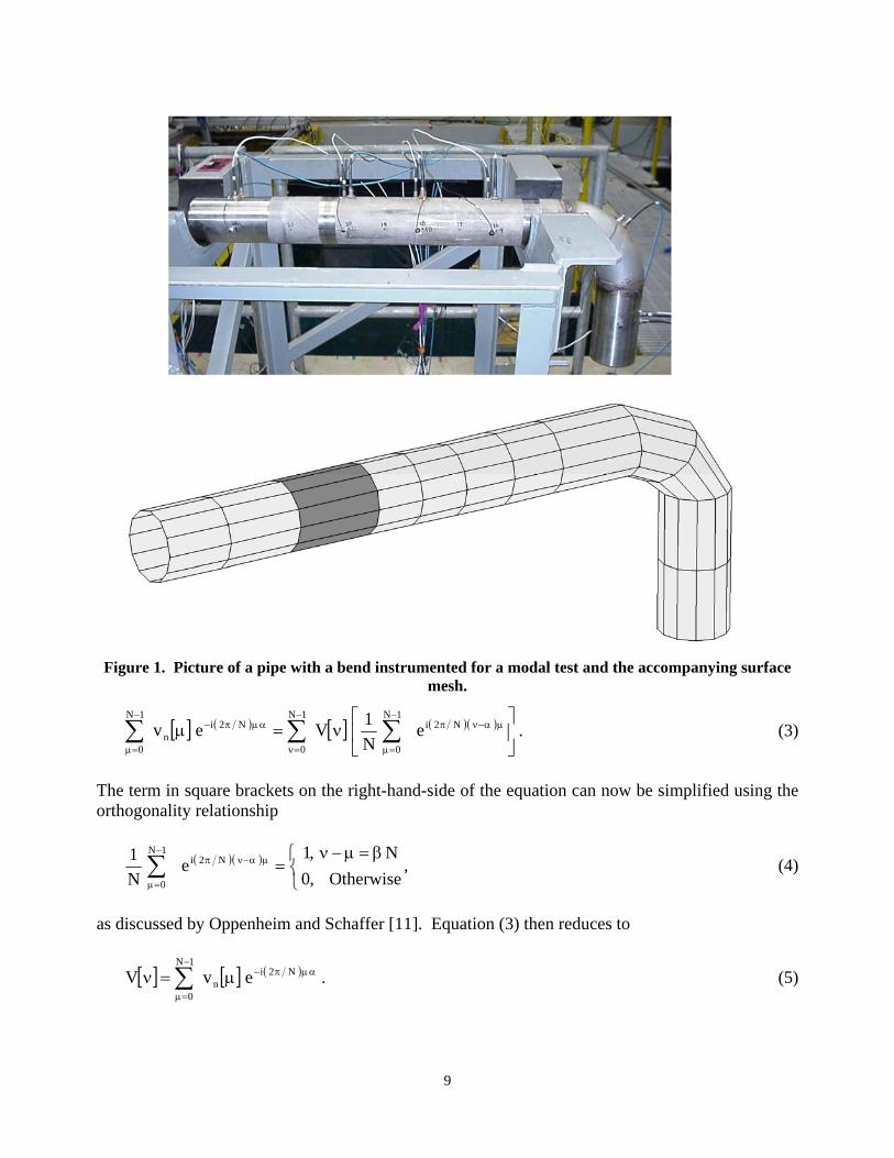
B. Discrete Fourier Series Decomposition During the execution of the computer program MODAL_ANALYSIS_USING_SVD, surface vibration profiles are computed for the various drive points prior to the modal identification process. It is often possible to gain considerable insight into the vibration of a structure with rotational symmetry by applying a discrete Fourier series spatial decomposition. For a structure with N angular sections, the normal velocity can be expanded as [10]

1N

0

N2in eV

N

1v , (1)

where the square brackets indicate discrete variables, and the V[] represent the Fourier coefficients for the expansion. In the present implementation, the calculations are performed using elementally averaged values, and thus a separate expansion is taken for every element in the first angular section. As discussed in the previous section, the calculations are performed for subsets of the element mesh, as input by the user in the files geom_fourier1.txt, geom_fourier2.txt, etc. It is assumed that the element mesh is numbered with all the data for the first angular section first, and the same element numbering scheme is used for the rest of the sections. To illustrate, Figure 1 shows a picture of a pipe with a bend that has been instrumented for a modal test. This same dataset will be used throughout this document to illustrate the various calculations. In the accompanying picture of the element mesh, the vibrations for the shaded elements, which are rotationally-symmetric about the centerline of the pipe, are used to compute the discrete Fourier transform. To solve for the Fourier

coefficients, both sides of Equation (1) are multiplied by exp i 2 N and summed from

= 0 to N-1 to yield

1N

0

1N

0

N2i1N

0

N2in eV

N

1ev . (2)

Switching the order of the summations on the right-hand-side gives

9

Figure 1. Picture of a pipe with a bend instrumented for a modal test and the accompanying surface mesh.

1N

0

1N

0

N2i1N

0

N2in e

N

1Vev . (3)

The term in square brackets on the right-hand-side of the equation can now be simplified using the orthogonality relationship

Otherwise,0

N,1e

N

1 1N

0

N2i , (4)

as discussed by Oppenheim and Schaffer [11]. Equation (3) then reduces to

1N

0

N2in evV . (5)

10

In the general case, the FFT algorithm is not used to speed up the calculations because N is not necessarily a multiple of 2. However, computational speed is rarely an issue, even for large sets of experimental data. In acoustic calculations, it is often useful to be able to calculate surface integrals of the squared normal velocity. It is possible to calculate a discrete Fourier series decomposition of the integrated squared normal velocity as well. To begin, the squared normal velocity can be written as

1N

0

N2i*1N

0

N2i2

n eVN

1eV

N

1v . (6)

Summing over and rearranging the right-hand-side gives

1N

0

N2i1N

0

*1N

02

1N

0

2

n eVVN

1v . (7)

From the orthogonality relationship in Equation (4), the inner-most summation yields N when = and zero otherwise. Thus, the triple summation reduces to a single summation as

1N

0

21N

0

2

n VN

1v . (8)

This result holds for each rotationally-symmetric element. To compute the full surface integration, the result in Equation (8) is multiplied by the appropriate element area and summed over all the elements in the first angular section, yielding

1N

0

2NES

1S

2

n VSN

1xSdxv , (9)

where NES is the number of elements in the first angular section. The Fourier transform can only resolve coefficients up to N / 2, and the coefficients are repeated about N / 2. To ensure that the coefficients will sum to yield the same overall total, the repeated coefficients are summed as 1NV0V0V , 2NV1V1V , etc. If N is an even number, the 2NV term is not

“mirrored” about N / 2 like the rest of the coefficients. The Fourier transform data is written in the files named either fourier?_dr_pt_?.txt (for the surface-averaged accelerance) or fourier_modes1.txt (for the mode shapes). To illustrate the calculations, modal data for a 3-inch diameter schedule 10 pipe with a bend, as shown in Figure 1, will be processed using the discrete Fourier series decomposition. In generating the data, acceleration-to-force transfer functions were measured at eight accelerometer locations for each impact location on the surface element mesh. Thus, the number of drive points (hammer impact locations) is much larger than the number of response points (accelerometer measurement locations). However, it is typically more useful to have a complete set of surface acceleration data for a relatively small number of drive points. Thus, for tests using a modal hammer and accelerometer, reciprocity

11

is often invoked, and the accelerometer locations are interpreted as the drive points and hammer impact locations are interpreted as the response points. By default, the computer program will “switch” the drive and response points so that there are always more response points. (As noted previously, the input parameter SW in the in.txt file can be used to switch the format so that the drive points outnumber the response points.)

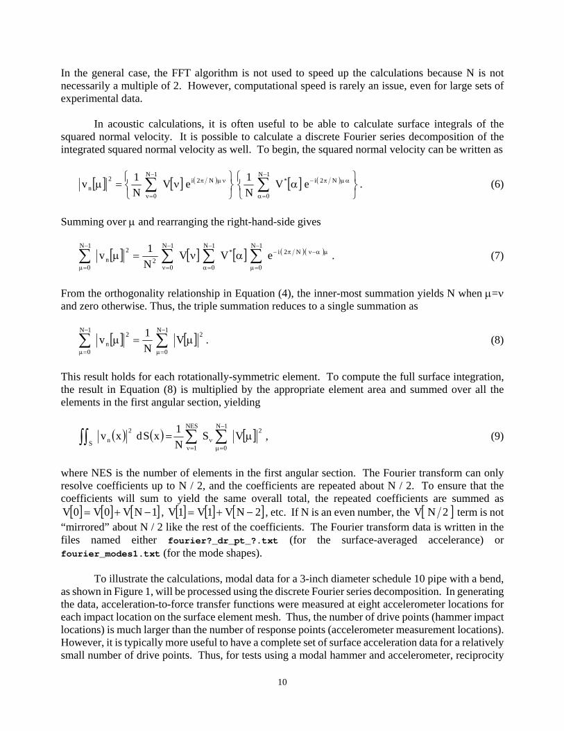
In processing the data for the shaded region of the pipe bend, there are 12 elements around the circumference of the pipe, and thus the transform yields coefficients for harmonics 0 through 5. Figure 2 shows the result for the Fourier series decomposition for drive point 47. For the pipe bend, the elements used for the decomposition are rotationally-symmetric about the centerline of the pipe, but the complete structure is not rotationally-symmetric. Thus, there is no reason to expect the various Fourier harmonics to be uncoupled. Still, it is possible to clearly discern the “cut-on” frequency for the N = 2 and N = 3 modes at approximately 1000 and 2700 Hz, respectively. Figure 3 shows a few mode shapes that occur just above the cut-on frequency for N = 3 modes. Because the pipe is rotationally symmetric about the centerline, circumferential harmonics higher than order 6

appear in the spectrum and will be aliased. For example, harmonic of order 7 will appear as peaks in the N = 1 spectrum. Aliasing is not an issue for the present analysis because the higher order harmonics occur above the frequency range of interest.

Figure 2. Discrete Fourier series decomposition of the vibrations of one ring of elements around the

pipe.

0 1000 2000 3000 4000 5000

Frequency, Hz

0

20

40

60

80

100

Inte

gra

ted

Sq

ua

red

No

rma

l Ve

loci

ty, d

B r

e 1

x 1

0-1

2 W

Total N = 0N = 1N = 2N = 3

12

Figure 3. Mode shapes for resonances clustered near the cut-on frequency for N = 3 modes.

If the measurement mesh is circumferentially-symmetric, it is also possible to use the circumferential Fourier series to filter the transfer function data before running program MODAL_ANALYSIS_USING_SVD to extract the modal parameters. This is mainly useful for helping to extract underlying modes when the modal density is high. The program used to filter the transfer function data is named FOURIER_FILTER, and it writes out a new file named exp_data_n?.bin , where ? is the retained Fourier harmonic. The parameter IO in the in.txt file chooses the harmonic to be retained after filtering. The program MODAL_ANALYSIS_USING_SVD is then run as usual with the filtered transfer function data. The Fourier transform computations should then reflect the fact that the data has been filtered, and this can be used to check that only one circumferential harmonic is present.

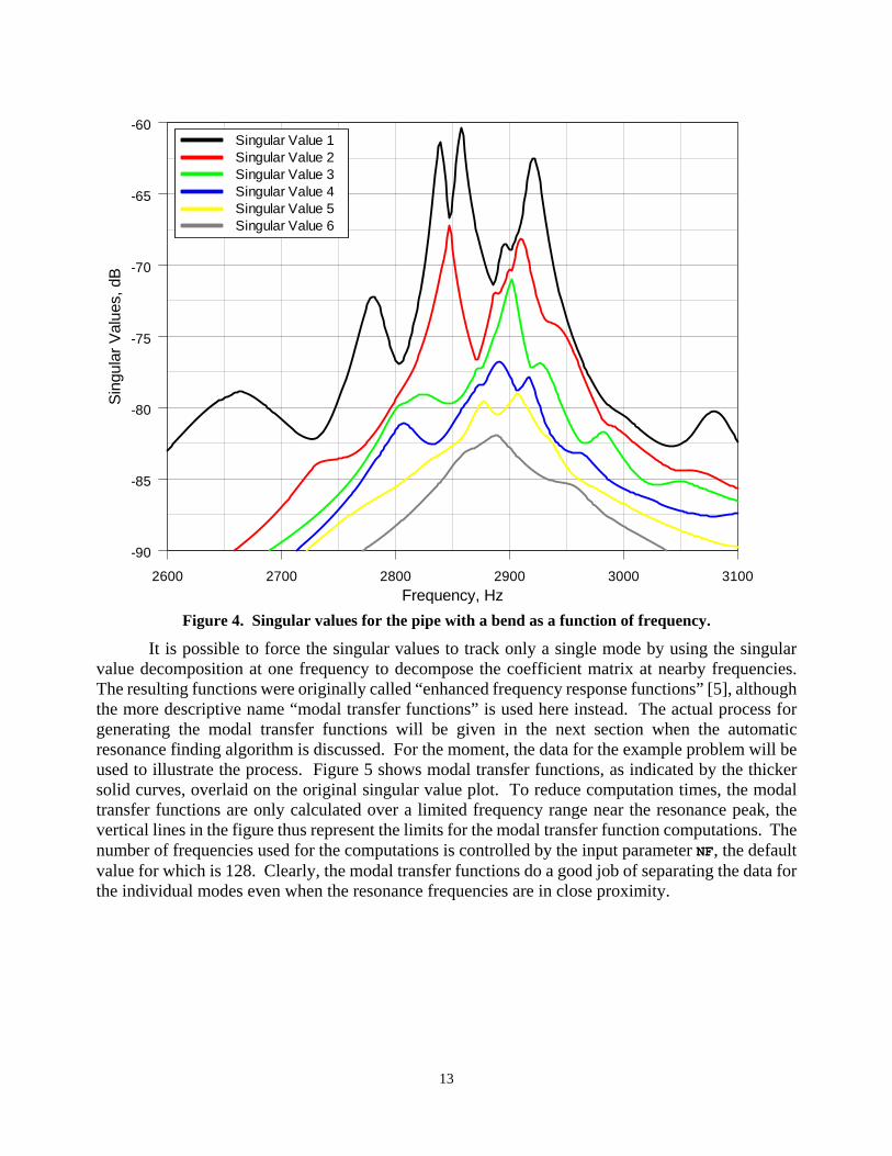
C. Application of the Singular Value Decomposition The key step in the modal analysis process is the application of the singular value decomposition to the transfer function or vibration data. In this section, the pipe bend data discussed in the previous section will be used to illustrate how the singular value decomposition is able to separate the modes from each other and how the data can be used to generate “modal transfer functions”. As mentioned in the introduction, the transfer function data is processed using the singular value decomposition one frequency at a time. The data is arranged in matrix form with each column representing the response to a different drive point and each row representing a different response point. The resulting matrix is input to the singular value decomposition algorithm and left- and right-singular vectors and a diagonal singular value matrix are computed. Figure 4 shows a plot of the singular values as a function of frequency for the pipe with a bend. Because they are computed and output in order of descending magnitude, a single curve on the plot does not track a single mode. For example, just below 2850 Hz, the top two curves switch the modes that they’re tracking. It is clear from this plot that the singular values contain modal information, but it is also clear that some processing is required before it can be extracted.

13

Figure 4. Singular values for the pipe with a bend as a function of frequency.

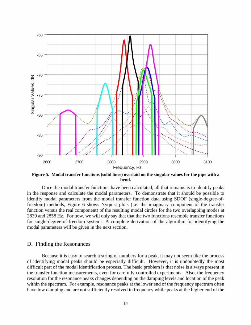
It is possible to force the singular values to track only a single mode by using the singular value decomposition at one frequency to decompose the coefficient matrix at nearby frequencies. The resulting functions were originally called “enhanced frequency response functions” [5], although the more descriptive name “modal transfer functions” is used here instead. The actual process for generating the modal transfer functions will be given in the next section when the automatic resonance finding algorithm is discussed. For the moment, the data for the example problem will be used to illustrate the process. Figure 5 shows modal transfer functions, as indicated by the thicker solid curves, overlaid on the original singular value plot. To reduce computation times, the modal transfer functions are only calculated over a limited frequency range near the resonance peak, the vertical lines in the figure thus represent the limits for the modal transfer function computations. The number of frequencies used for the computations is controlled by the input parameter NF, the default value for which is 128. Clearly, the modal transfer functions do a good job of separating the data for the individual modes even when the resonance frequencies are in close proximity.

2600 2700 2800 2900 3000 3100

Frequency, Hz

-90

-85

-80

-75

-70

-65

-60S

ingu

lar

Val

ues,

dB

Singular Value 1 Singular Value 2 Singular Value 3 Singular Value 4 Singular Value 5 Singular Value 6

14

Figure 5. Modal transfer functions (solid lines) overlaid on the singular values for the pipe with a bend.

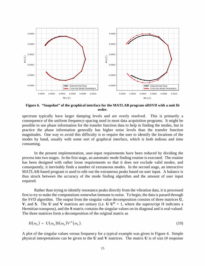
Once the modal transfer functions have been calculated, all that remains is to identify peaks in the response and calculate the modal parameters. To demonstrate that it should be possible to identify modal parameters from the modal transfer function data using SDOF (single-degree-of-freedom) methods, Figure 6 shows Nyquist plots (i.e. the imaginary component of the transfer function versus the real component) of the resulting modal circles for the two overlapping modes at 2839 and 2858 Hz. For now, we will only say that that the two functions resemble transfer functions for single-degree-of-freedom systems. A complete derivation of the algorithm for identifying the modal parameters will be given in the next section.

D. Finding the Resonances Because it is easy to search a string of numbers for a peak, it may not seem like the process of identifying modal peaks should be especially difficult. However, it is undoubtedly the most difficult part of the modal identification process. The basic problem is that noise is always present in the transfer function measurements, even for carefully controlled experiments. Also, the frequency resolution for the resonance peaks changes depending on the damping levels and location of the peak within the spectrum. For example, resonance peaks at the lower end of the frequency spectrum often have low damping and are not sufficiently resolved in frequency while peaks at the higher end of the

2600 2700 2800 2900 3000 3100

Frequency, Hz

-90

-85

-80

-75

-70

-65

-60S

ing

ula

r V

alu

es,

dB

15

spectrum typically have larger damping levels and are overly resolved. This is primarily a consequence of the uniform frequency-spacing used in most data acquisition programs. It might be possible to use phase information for the transfer function data to help in finding the modes, but in practice the phase information generally has higher noise levels than the transfer function magnitudes. One way to avoid this difficulty is to require the user to identify the locations of the modes by hand, usually with some sort of graphical interface, which is both tedious and time consuming.

In the present implementation, user-input requirements have been reduced by dividing the

process into two stages. In the first stage, an automatic mode finding routine is executed. The routine has been designed with rather loose requirements so that it does not exclude valid modes, and consequently, it inevitably finds a number of extraneous modes. In the second stage, an interactive MATLAB-based program is used to edit out the extraneous peaks based on user input. A balance is thus struck between the accuracy of the mode finding algorithm and the amount of user input required.

Rather than trying to identify resonance peaks directly from the vibration data, it is processed first to try to make the computations somewhat immune to noise. To begin, the data is passed through the SVD algorithm. The output from the singular value decomposition consists of three matrices U, V, and S. The U and V matrices are unitary (i.e. U UH = 1, where the superscript H indicates a Hermitian transpose), and the S matrix contains the singular values on its diagonal and is real-valued. The three matrices form a decomposition of the original matrix as 0000 VSUH H . (10)

A plot of the singular values versus frequency for a typical example was given in Figure 4. Simple physical interpretations can be given to the U and V matrices. The matrix U is of size (# response

Figure 6. “Snapshot” of the graphical interface for the MATLAB program siftSVD with a unit fit

order.

0.0000 0.0002 0.0004 0.0006 0.0008 0.0010

Re { Z }

-0.0005

-0.0003

-0.0001

0.0001

0.0003

0.0005

Im {

Z }

Experimental Data From the Modal Parameters

0.0000 0.0002 0.0004 0.0006 0.0008 0.0010

Re { Z }

-0.0005

-0.0003

-0.0001

0.0001

0.0003

0.0005

Im {

Z }

Experimental Data From the Modal Parameters

16

points) by (# drive points), and its columns (termed left-singular vectors) represent the vibration patterns associated with each of the singular values, and thus are interpreted as “unscaled mode shapes”. When we refer subsequently to “SVD mode shapes”, we really are referring to the left-singular vector associated with the singular value under consideration. The matrix V is of size (# drive points) by (# drive points), and its columns (termed right singular vectors) represent the required input forces at the drive points to excite the left-singular vectors. In general, the U and V matrices do not change significantly from one frequency to the next, and thus most of the frequency dependence in the transfer function data is contained in the singular values.

The SVD algorithm relegates noise to the lowest singular values, thus reducing the noise levels in the top few curves that typically contain most of the modal information. Unfortunately, the singular values are output from the decomposition in order of magnitude, so that they switch the modes they are tracking whenever two singular values cross. This problem is avoided by computing modal transfer functions, which force the singular values to track a single mode. These functions are computed by using the singular value decomposition at an initial frequency to decompose the transfer function matrix at nearby frequencies as 00

H VHUS . (11)

The overbar on the matrix S indicates that it is no longer real-valued or diagonal. At the initial frequency 0 , the modal transfer function yields 0S because pre-multiplying by 0

H U and

post-multiplying by 0V yields

0000

H000

H000

H SISIVVSUUVHU . (12)

A plot of the modal transfer functions versus frequency for the pipe bend example was given in Figure 5. Even after passing the data through the SVD algorithm, it is not uncommon for the noise levels in the modal transfer function data to be too high for a simple peak finding algorithm to work reliably.

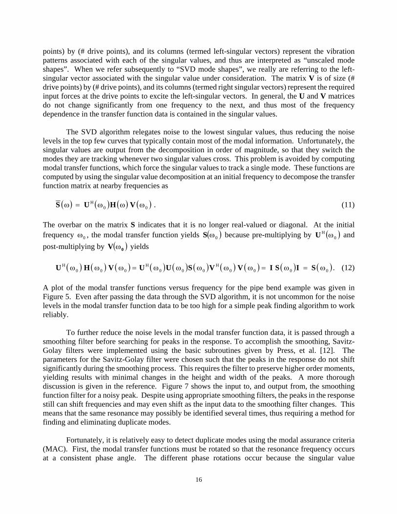
To further reduce the noise levels in the modal transfer function data, it is passed through a smoothing filter before searching for peaks in the response. To accomplish the smoothing, Savitz-Golay filters were implemented using the basic subroutines given by Press, et al. [12]. The parameters for the Savitz-Golay filter were chosen such that the peaks in the response do not shift significantly during the smoothing process. This requires the filter to preserve higher order moments, yielding results with minimal changes in the height and width of the peaks. A more thorough discussion is given in the reference. Figure 7 shows the input to, and output from, the smoothing function filter for a noisy peak. Despite using appropriate smoothing filters, the peaks in the response still can shift frequencies and may even shift as the input data to the smoothing filter changes. This means that the same resonance may possibly be identified several times, thus requiring a method for finding and eliminating duplicate modes.

Fortunately, it is relatively easy to detect duplicate modes using the modal assurance criteria

(MAC). First, the modal transfer functions must be rotated so that the resonance frequency occurs at a consistent phase angle. The different phase rotations occur because the singular value

17

decomposition yields real singular values, such that zero phase is always referenced to the frequency used to generate the modal transfer functions. To accomplish the rotation without any user input, a circle-fit algorithm is used to determine the best fit for the center of the modal circle and its diameter. This information can then be used to adjust the phase at the resonance peak.

To begin the analysis, the modal circle is assumed to have radius R0 and centerpoint (x0, y0).

Using one of the raw “unsmoothed” modal transfer function curves for N frequencies as input, the formula for the error in the circle fit is given as [13]

N

1

220

20

20 yyxxRE , SImy,SRex . (13)

This can be rewritten as

N

1

222 yybxaxcE , 20

20

20 yxRc (14)

Minimizing with respect to a, b, and c yields

Figure 7. Input to, and output from, the Savitz-Golay smoothing filter.

3030 3040 3050 3060 3070 3080 3090

Frequency, Hz

-35

-34

-33

-32

-31

-301

/ Sin

gula

r V

alue

s, d

B

Input Output

18

N

1

22

N

1

23

N

1

23

N

1

N

1

N

1

N

1

2N

1

N

1

N

1

N

1

2

yx

xyy

yxx

c

b

a

Nyx

yyyx

xyxx

. (15)

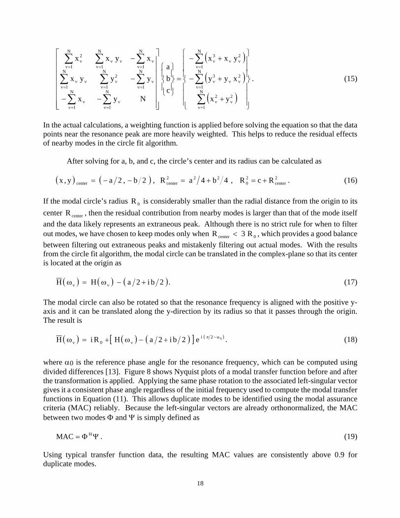
In the actual calculations, a weighting function is applied before solving the equation so that the data points near the resonance peak are more heavily weighted. This helps to reduce the residual effects of nearby modes in the circle fit algorithm.

After solving for a, b, and c, the circle’s center and its radius can be calculated as 2

center20

222centercenter RcR,4b4aR,2b,2ay,x . (16)

If the modal circle’s radius 0R is considerably smaller than the radial distance from the origin to its

center centerR , then the residual contribution from nearby modes is larger than that of the mode itself

and the data likely represents an extraneous peak. Although there is no strict rule for when to filter out modes, we have chosen to keep modes only when 0center R3R , which provides a good balance

between filtering out extraneous peaks and mistakenly filtering out actual modes. With the results from the circle fit algorithm, the modal circle can be translated in the complex-plane so that its center is located at the origin as 2bi2aHH . (17)

The modal circle can also be rotated so that the resonance frequency is aligned with the positive y-axis and it can be translated along the y-direction by its radius so that it passes through the origin. The result is 02i

0 e2bi2aHRiH . (18)

where 0 is the reference phase angle for the resonance frequency, which can be computed using divided differences [13]. Figure 8 shows Nyquist plots of a modal transfer function before and after the transformation is applied. Applying the same phase rotation to the associated left-singular vector gives it a consistent phase angle regardless of the initial frequency used to compute the modal transfer functions in Equation (11). This allows duplicate modes to be identified using the modal assurance criteria (MAC) reliably. Because the left-singular vectors are already orthonormalized, the MAC between two modes and is simply defined as HMAC . (19) Using typical transfer function data, the resulting MAC values are consistently above 0.9 for duplicate modes.

19

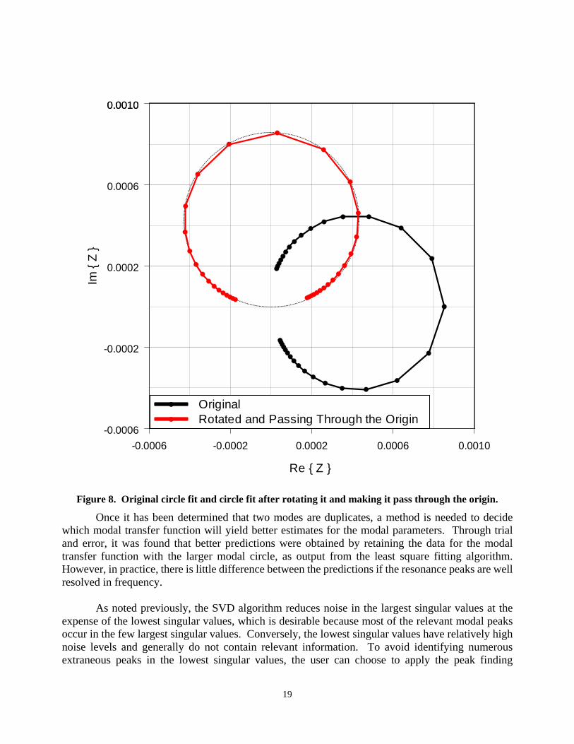
Figure 8. Original circle fit and circle fit after rotating it and making it pass through the origin.

Once it has been determined that two modes are duplicates, a method is needed to decide which modal transfer function will yield better estimates for the modal parameters. Through trial and error, it was found that better predictions were obtained by retaining the data for the modal transfer function with the larger modal circle, as output from the least square fitting algorithm. However, in practice, there is little difference between the predictions if the resonance peaks are well resolved in frequency. As noted previously, the SVD algorithm reduces noise in the largest singular values at the expense of the lowest singular values, which is desirable because most of the relevant modal peaks occur in the few largest singular values. Conversely, the lowest singular values have relatively high noise levels and generally do not contain relevant information. To avoid identifying numerous extraneous peaks in the lowest singular values, the user can choose to apply the peak finding

-0.0006 -0.0002 0.0002 0.0006 0.0010

Re { Z }

-0.0006

-0.0002

0.0002

0.0006

0.0010Im

{ Z

}

Original Rotated and Passing Through the Origin

0.0010

20

algorithm to only a few of the largest singular values. The parameter NP in the text input file in.txt, an example of which is listed in Appendix A, is used to specify the number of singular values to search for peaks. As a general rule, the lowest singular value should always be excluded from the search. If the code stops because the array VSQ_MODE is out of bounds, the number of singular values to search for response peaks should be reduced.

E. Modal Parameter Identification The last step in the process is to actually determine the resonance frequencies and loss factors from the modal data. There are many methods for computing the modal parameters once the data for a single mode has been isolated. In the present implementation, a simple least squares method for determining the parameters is used. The basic idea is to assume the modal transfer function for mode can be represented in the form (assuming a i te sign convention)

22 2 2 2

A AH , B 1 i

i B

. (20)

where A and B are complex-valued constants. The reciprocal of the modal transfer function can then be written as

221

2 ccBA

1

H

1

. (21)

In this form, the constant can be determined using linear least squares, making the solution much more reliable and efficient than an iterative nonlinear least squares solution. The error in the least square fit is calculated as

2

N

1

221 cc

H

1E

. (22)

Taking the derivative with respect to the constants gives

2

N

1

221

2

N

1

221

1

ccH

12

c

E

ccH

12

c

E

. (23)

Setting the derivatives equal to zero and rewriting the equations to solve for the constants gives the normal equations as

21

N

1

2

N

1

2

1N

1

4N

1

2

N

1

2

H

H1

c

cN. (24)

Solving for the constants yields the resonance frequency and loss factor as:

22 1 1 2A 1 c , B A c c c , Re B , Im B . (25)

As for the circle fit algorithm, a weighting function is applied before solving the equation system so that the data points near the resonance peak are more heavily weighted. Once the resonance frequency and damping loss factor have been determined, the modal transfer function can be synthesized and compared to the input data to assess the accuracy of the fit. To try to make the predictions more reliable and immune to noise, these calculations are performed for different numbers of input frequencies surrounding the resonance frequency, and the fit with the lowest average error is used for the predictions. If the modal transfer functions are relatively free of noise, the fit is typically better using only a few points near the peak, otherwise, better results are obtained using more data. The program MODAL_ANALYSIS_USING_SVD writes several files giving the results of the modal analysis. Most of the files are used primarily as input for the subsequent analysis in MATLAB using the program siftSVD, which is discussed in Sections G and H. The resonance frequencies and loss factors are written to a file named damp.txt along with some other diagnostic information, including the SVD order for each of the modes. At this stage, the resonance frequencies and loss factors are generally good estimates, but their accuracy is improved subsequently. Similarly, files are also written for the mode shapes (if the in.txt input parameter PP is set to 3), but again, they are primarily used as input to the subsequent calculations. Finally, the singular values of the transfer function matrix for each analysis frequency are written to a file named svd.txt. It is often useful to plot the data in the file as the program is running to check the quality of the experimental measurements. For example, it is usually immediately evident if one or more of the accelerometers did not function properly during the measurements because some or all of the singular values will appear “noisy”. In this situation, it is best to use coherence data to eliminate the bad data before performing the singular value decomposition, as discussed previously in Section A.

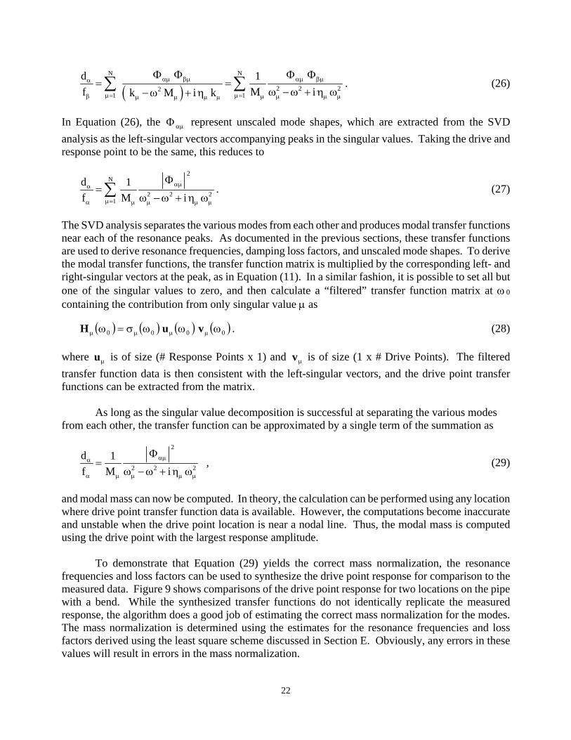
F. Mass Normalization within MODAL_ANALYSIS_USING_SVD While the scaling of the identified mode shapes is arbitrary, a mass-normalized set enables the measured data to be synthesized without knowledge of the system mass or stiffness characteristics. Therfore, in this section, the mass normalization within the program MODAL_ANALYSIS_USING_SVD is documented. To start, the transfer function between the displacement at node due to an input force at node can be written in the form (Ewins [1], pg. 55)

22

N N

2 2 221 1

d 1

f M ik M i k

. (26)

In Equation (26), the represent unscaled mode shapes, which are extracted from the SVD

analysis as the left-singular vectors accompanying peaks in the singular values. Taking the drive and response point to be the same, this reduces to

2N

2 2 21

d 1

f M i

. (27)

The SVD analysis separates the various modes from each other and produces modal transfer functions near each of the resonance peaks. As documented in the previous sections, these transfer functions are used to derive resonance frequencies, damping loss factors, and unscaled mode shapes. To derive the modal transfer functions, the transfer function matrix is multiplied by the corresponding left- and right-singular vectors at the peak, as in Equation (11). In a similar fashion, it is possible to set all but one of the singular values to zero, and then calculate a “filtered” transfer function matrix at 0 containing the contribution from only singular value as

0000 vuH . (28)

where u is of size (# Response Points x 1) and v is of size (1 x # Drive Points). The filtered

transfer function data is then consistent with the left-singular vectors, and the drive point transfer functions can be extracted from the matrix.

As long as the singular value decomposition is successful at separating the various modes

from each other, the transfer function can be approximated by a single term of the summation as

2

2 2 2

d 1

f M i

, (29)

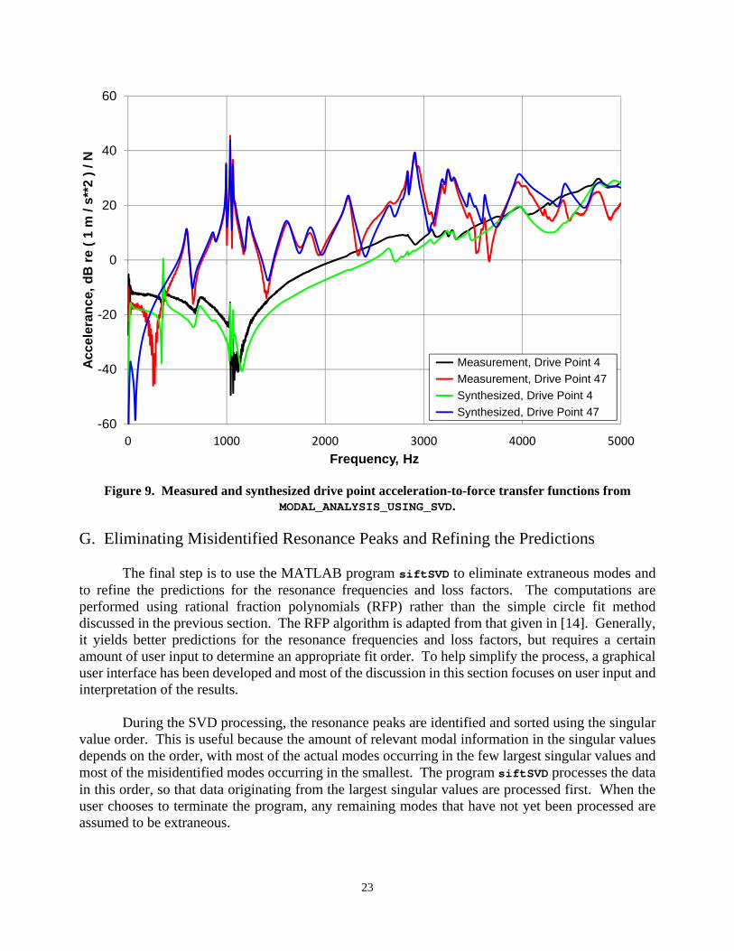
and modal mass can now be computed. In theory, the calculation can be performed using any location where drive point transfer function data is available. However, the computations become inaccurate and unstable when the drive point location is near a nodal line. Thus, the modal mass is computed using the drive point with the largest response amplitude. To demonstrate that Equation (29) yields the correct mass normalization, the resonance frequencies and loss factors can be used to synthesize the drive point response for comparison to the measured data. Figure 9 shows comparisons of the drive point response for two locations on the pipe with a bend. While the synthesized transfer functions do not identically replicate the measured response, the algorithm does a good job of estimating the correct mass normalization for the modes. The mass normalization is determined using the estimates for the resonance frequencies and loss factors derived using the least square scheme discussed in Section E. Obviously, any errors in these values will result in errors in the mass normalization.

23

Figure 9. Measured and synthesized drive point acceleration-to-force transfer functions from MODAL_ANALYSIS_USING_SVD.

G. Eliminating Misidentified Resonance Peaks and Refining the Predictions

The final step is to use the MATLAB program siftSVD to eliminate extraneous modes and to refine the predictions for the resonance frequencies and loss factors. The computations are performed using rational fraction polynomials (RFP) rather than the simple circle fit method discussed in the previous section. The RFP algorithm is adapted from that given in [14]. Generally, it yields better predictions for the resonance frequencies and loss factors, but requires a certain amount of user input to determine an appropriate fit order. To help simplify the process, a graphical user interface has been developed and most of the discussion in this section focuses on user input and interpretation of the results.

During the SVD processing, the resonance peaks are identified and sorted using the singular

value order. This is useful because the amount of relevant modal information in the singular values depends on the order, with most of the actual modes occurring in the few largest singular values and most of the misidentified modes occurring in the smallest. The program siftSVD processes the data in this order, so that data originating from the largest singular values are processed first. When the user chooses to terminate the program, any remaining modes that have not yet been processed are assumed to be extraneous.

-60

-40

-20

0

20

40

60

0 1000 2000 3000 4000 5000

Acc

eler

ance

, d

B r

e (

1 m

/ s

**2

) / N

Frequency, Hz

Measurement, Drive Point 4

Measurement, Drive Point 47

Synthesized, Drive Point 4

Synthesized, Drive Point 47

24

To start the program, the user changes the Matlab working directory (with the command cd) to the folder where the experimental data resides and then executes the command siftSVD (the path in MATLAB may have to be modified to include the folder Y:\Common\Noise Control and

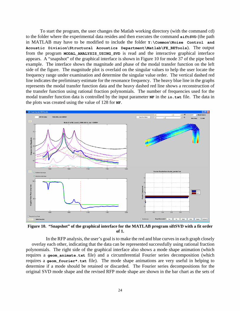
Acoustic Division\Structural Acoustics Department\Matlab\FE_BETools). The output from the program MODAL_ANALYSIS_USING_SVD is read and the interactive graphical interface appears. A “snapshot” of the graphical interface is shown in Figure 10 for mode 37 of the pipe bend example. The interface shows the magnitude and phase of the modal transfer function on the left side of the figure. The magnitude plot is overlaid on the singular values to help the user locate the frequency range under examination and determine the singular value order. The vertical dashed red line indicates the preliminary estimate for the resonance frequency. The heavy blue line in the graphs represents the modal transfer function data and the heavy dashed red line shows a reconstruction of the transfer function using rational fraction polynomials. The number of frequencies used for the modal transfer function data is controlled by the input parameter NF in the in.txt file. The data in the plots was created using the value of 128 for NF.

Figure 10. “Snapshot” of the graphical interface for the MATLAB program siftSVD with a fit order of 1.

In the RFP analysis, the user’s goal is to make the red and blue curves in each graph closely overlay each other, indicating that the data can be represented successfully using rational fraction

polynomials. The right side of the graphical interface also shows a mode shape animation (which requires a geom_animate.txt file) and a circumferential Fourier series decomposition (which requires a geom_fourier*.txt file). The mode shape animations are very useful in helping to determine if a mode should be retained or discarded. The Fourier series decompositions for the original SVD mode shape and the revised RFP mode shape are shown in the bar chart as the sets of

25

blue and red lines, respectively. The “mode source” edit box in the top right-hand corner of the figure allows the user to choose whether the original SVD or revised RFP mode shape is animated.

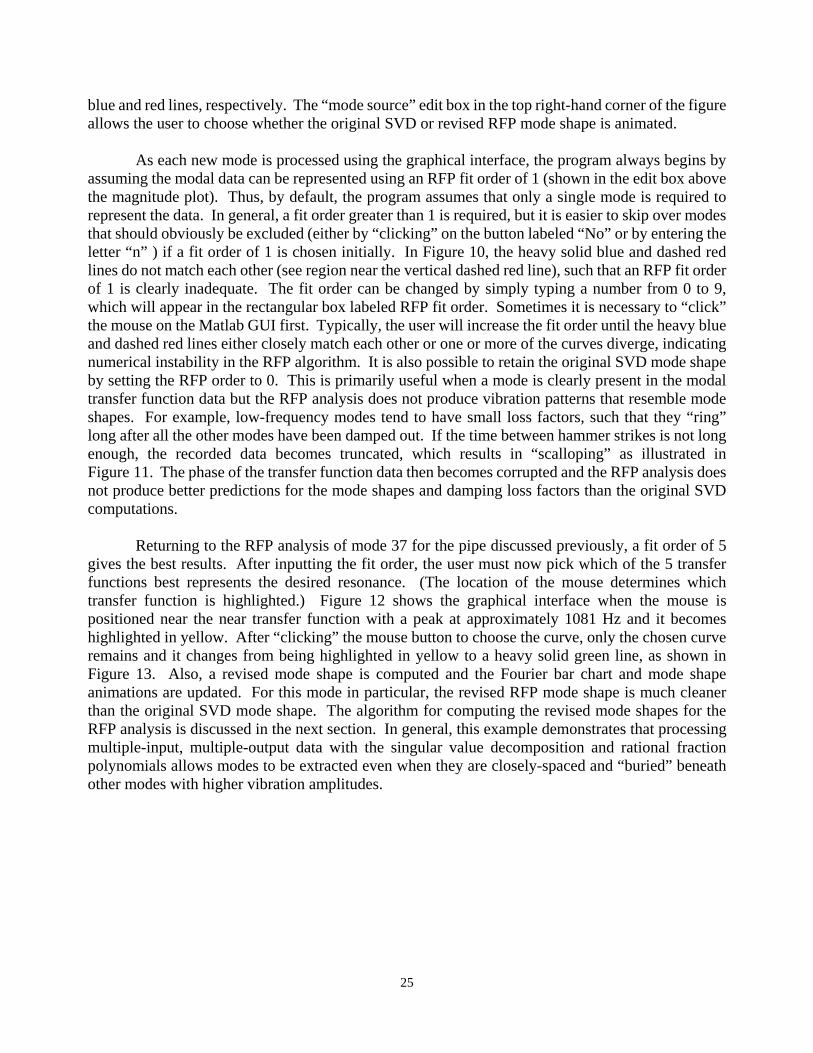
As each new mode is processed using the graphical interface, the program always begins by assuming the modal data can be represented using an RFP fit order of 1 (shown in the edit box above the magnitude plot). Thus, by default, the program assumes that only a single mode is required to represent the data. In general, a fit order greater than 1 is required, but it is easier to skip over modes that should obviously be excluded (either by “clicking” on the button labeled “No” or by entering the letter “n” ) if a fit order of 1 is chosen initially. In Figure 10, the heavy solid blue and dashed red lines do not match each other (see region near the vertical dashed red line), such that an RFP fit order of 1 is clearly inadequate. The fit order can be changed by simply typing a number from 0 to 9, which will appear in the rectangular box labeled RFP fit order. Sometimes it is necessary to “click” the mouse on the Matlab GUI first. Typically, the user will increase the fit order until the heavy blue and dashed red lines either closely match each other or one or more of the curves diverge, indicating numerical instability in the RFP algorithm. It is also possible to retain the original SVD mode shape by setting the RFP order to 0. This is primarily useful when a mode is clearly present in the modal transfer function data but the RFP analysis does not produce vibration patterns that resemble mode shapes. For example, low-frequency modes tend to have small loss factors, such that they “ring” long after all the other modes have been damped out. If the time between hammer strikes is not long enough, the recorded data becomes truncated, which results in “scalloping” as illustrated in Figure 11. The phase of the transfer function data then becomes corrupted and the RFP analysis does not produce better predictions for the mode shapes and damping loss factors than the original SVD computations.

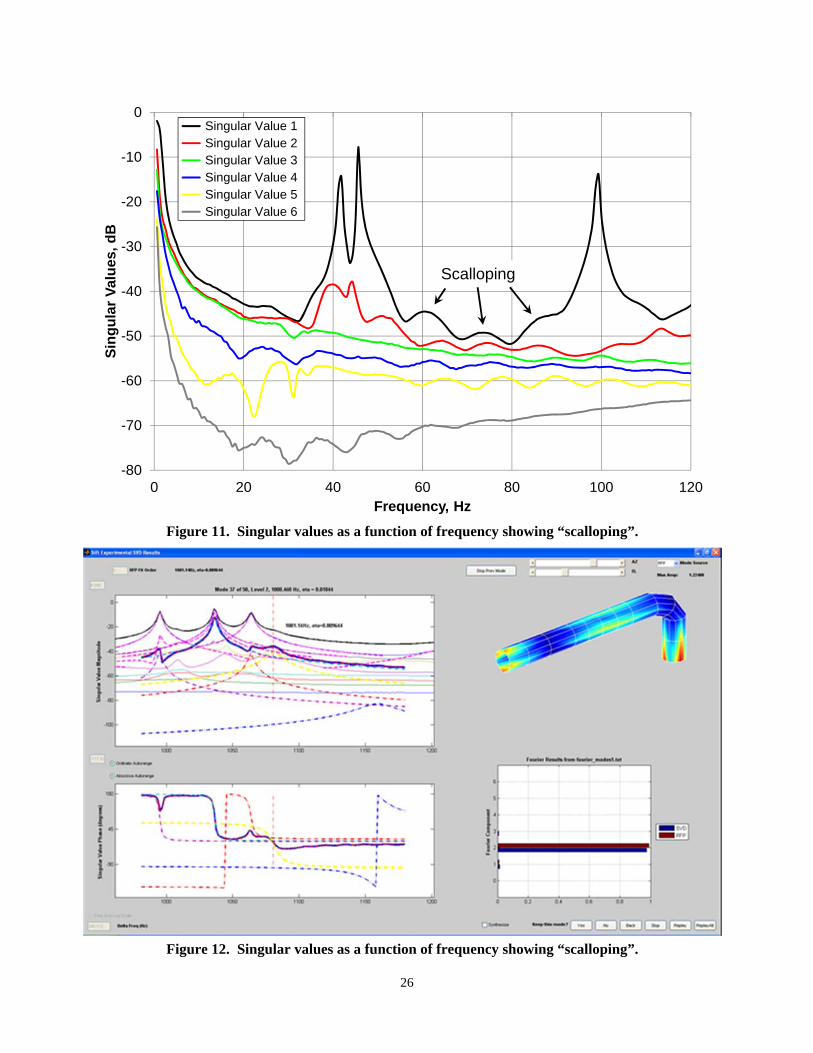
Returning to the RFP analysis of mode 37 for the pipe discussed previously, a fit order of 5

gives the best results. After inputting the fit order, the user must now pick which of the 5 transfer functions best represents the desired resonance. (The location of the mouse determines which transfer function is highlighted.) Figure 12 shows the graphical interface when the mouse is positioned near the near transfer function with a peak at approximately 1081 Hz and it becomes highlighted in yellow. After “clicking” the mouse button to choose the curve, only the chosen curve remains and it changes from being highlighted in yellow to a heavy solid green line, as shown in Figure 13. Also, a revised mode shape is computed and the Fourier bar chart and mode shape animations are updated. For this mode in particular, the revised RFP mode shape is much cleaner than the original SVD mode shape. The algorithm for computing the revised mode shapes for the RFP analysis is discussed in the next section. In general, this example demonstrates that processing multiple-input, multiple-output data with the singular value decomposition and rational fraction polynomials allows modes to be extracted even when they are closely-spaced and “buried” beneath other modes with higher vibration amplitudes.

26

Figure 11. Singular values as a function of frequency showing “scalloping”.

Figure 12. Singular values as a function of frequency showing “scalloping”.

-80

-70

-60

-50

-40

-30

-20

-10

0

0 20 40 60 80 100 120

Sin

gu

lar

Val

ues

, d

B

Frequency, Hz

Singular Value 1 Singular Value 2 Singular Value 3 Singular Value 4 Singular Value 5 Singular Value 6

Scalloping

27

In addition to choosing the proper fit order, the user also has to determine when to exclude misidentified modes. In many instances, the choice is obvious. However, there are also many instances where the choice of whether or not to eliminate a mode is somewhat subjective. As a general guideline, if the vertical red line in the figure marking the resonance frequency does not line up with a peak in the modal transfer function, then the data likely represents an extraneous peak. Similarly, if the phase does not go through a 180 degree shift near the resonance peak, it should also be omitted. Many times, the singular value decomposition is not able to isolate the modal information for a resonance peak within a single singular value. Peaks will then occur for several singular values at the same frequency with very similar modal transfer functions. This is especially true if the overall coherence level is relatively low. In this circumstance, the best way to ensure that the same mode is not included more than once is using the “Display Previous Mode” button. When this button is picked, one of three things happens. Nothing happens if no previously identified modes (displayed as dashed lines) appear in the current window. If only one previously identified mode appears, then the mode shape is animated in separate window. Finally, if more than one previously identified mode appears in the current window, the user is prompted to pick the desired mode to display. The header for the window lists the resonance frequency, damping loss factor, and the MAC (modal assurance criteria) between the previously identified mode and the one under consideration. To illustrate, Figure 14 shows a set of duplicate modes that are found near 1080 Hz for singular values 2 and 3. The separate window shows the mode that was found for singular value 2, and the mode under consideration for singular value 3 is shown above it. The MAC between the two modes is above 0.9, so they are clearly duplicates, and the mode under consideration should be eliminated from the mode set by choosing the button labeled “No”, such that only the mode previously identified for singular value 2 is retained.

Figure 13. “Snapshot” of the graphical interface after picking the desired mode.

28

There are also situations in which modes are mistakenly identified or identified more than once. The concept of “modal transfer functions” was developed to avoid difficulties when two singular values switch the vibration patterns that they are tracking, as discussed previously in Section D. Unfortunately, this does not completely eliminate the problem, and occasionally a mode is mistakenly identified at a frequency where two singular values cross. When this happens, the same mode will not be consistently identified for different RFP orders, and the mode should be eliminated. Similarly, the algorithm for eliminating duplicate modes using the MAC does not always work and the same resonance peak will be represented more than once. When this happens, the user can verify that the same mode is being identified more than once using the “Display Previous Mode” button. The modal transfer function with smaller residual contributions from nearby modes should then be used for the RFP analysis and to compute the mode shape.

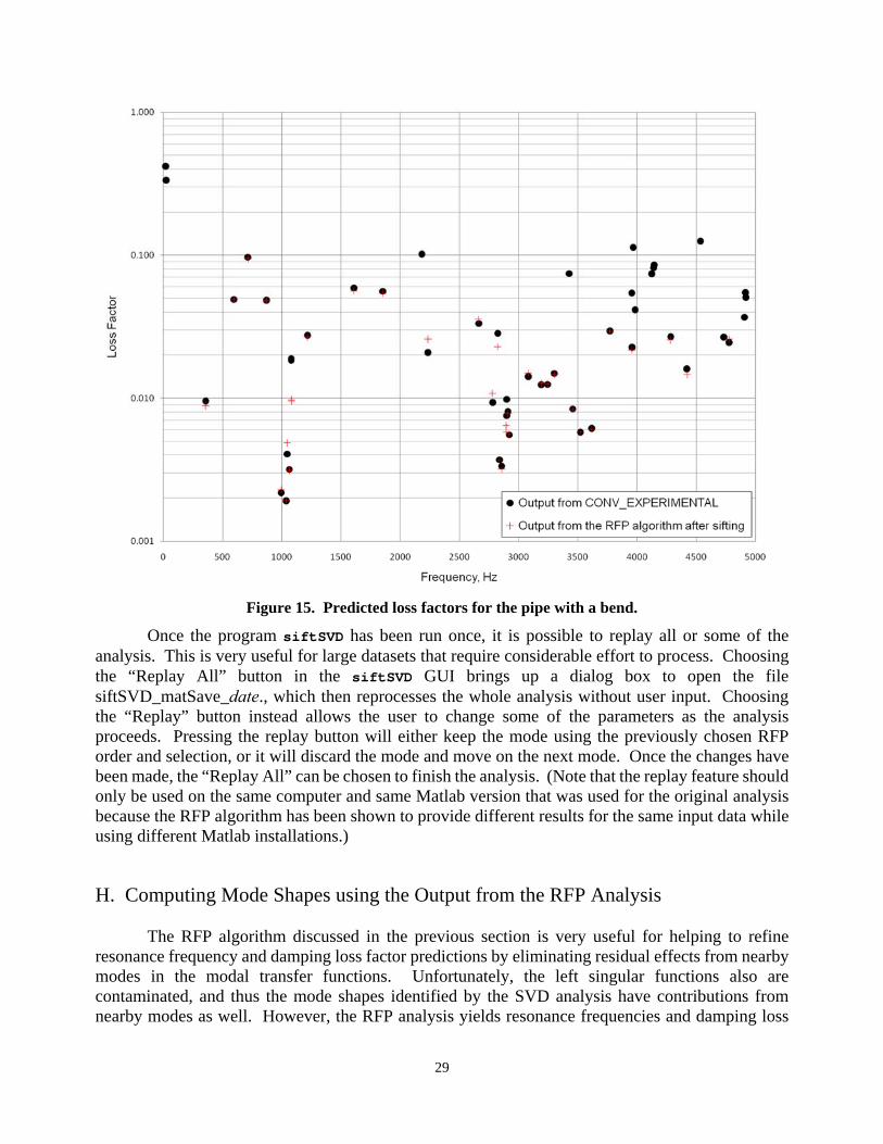
Once all the modes have been processed, the program siftSVD rearranges the modes in order of increasing frequency and writes versions of the input damp.txt and fourier_modes?.txt files that only include the retained modes (with _sifted added into the name before the file extension). Figure 15 shows the final results for the resonance frequencies and damping loss factors for the pipe with a bend. In this example, most of the misidentified modes occur at the higher end of the frequency spectrum, as indicated by black dots without corresponding red crosses. However, the noise levels were very low for this test, and it is common for the low frequency response to contain numerous peaks due to noise contamination. Thus, in general, the majority of the misidentified modes occur at the low and high ends of the frequency spectrum.

Figure 14. “Snapshot” of the graphical interface when using the “Display Previous Mode” button.

29

Figure 15. Predicted loss factors for the pipe with a bend.

Once the program siftSVD has been run once, it is possible to replay all or some of the analysis. This is very useful for large datasets that require considerable effort to process. Choosing the “Replay All” button in the siftSVD GUI brings up a dialog box to open the file siftSVD_matSave_date., which then reprocesses the whole analysis without user input. Choosing the “Replay” button instead allows the user to change some of the parameters as the analysis proceeds. Pressing the replay button will either keep the mode using the previously chosen RFP order and selection, or it will discard the mode and move on the next mode. Once the changes have been made, the “Replay All” can be chosen to finish the analysis. (Note that the replay feature should only be used on the same computer and same Matlab version that was used for the original analysis because the RFP algorithm has been shown to provide different results for the same input data while using different Matlab installations.)

H. Computing Mode Shapes using the Output from the RFP Analysis

The RFP algorithm discussed in the previous section is very useful for helping to refine resonance frequency and damping loss factor predictions by eliminating residual effects from nearby modes in the modal transfer functions. Unfortunately, the left singular functions also are contaminated, and thus the mode shapes identified by the SVD analysis have contributions from nearby modes as well. However, the RFP analysis yields resonance frequencies and damping loss

30

factors for the desired resonance as well as the residual modes, and this information can be used to extract more accurate mode shapes.

To extract mode shape information using rational fraction polynomials, filtered transfer

functions are required over the frequency range of interest for each node. At the analysis frequency

0 , the singular value decomposition can be used to filter the transfer function matrix for one of the

singular values as given previously in Equation (28). Each column of the transfer function matrix represents the response vector for one of the drive points. When the structure is driven at the point that produces the maximum response, the operating deflections for singular value are given by *

0 0 max, 0 0s v h u . (30)

where h is column of H, *

max,v is the maximum value in column of V, and u is column of U.

This simple formula is only valid at the analysis frequency. However, operating deflection shapes can be computed over a frequency range near the resonance using the singular value decomposition at 0 in the same way that modal transfer functions were computed previously. This is done by

premultiplying Equation (11) by 0U to yield

0 0 U S H V . (31)

In physical terms, this equation can be thought of in either of two ways. The left side of the equation represents the static mode shapes multiplied by the complex singular value matrix, which contains most of the frequency information. Thus, one column will resemble a mode shape multiplied by its associated modal transfer function and is similar to an operating deflection shape. However, because

S is not diagonal, the operating deflection shapes change for each response node. The right side

of the equation gives another interpretation. The columns of 0V represent the optimum input

forces to excite each of the left singular vectors. Extracting column on each side of Equation (31) yields 0 0 U s H v . (32)

At 0 , the left side of Equation (32) reduces to 0 0s u , so that the generalized version of

Equation (30) is given as * *

max, 0 0 max, 0 0v v h U s H v . (33)

Since 0 H v is already computed as part of the modal transfer function calculation, all that

is required is to extract the data for singular value when a mode is identified and multiply it by

*max, 0v to yield h . The end result is a complex-valued transfer function for each response

point over the frequency range near the resonance. An examination of the data shows that the

31

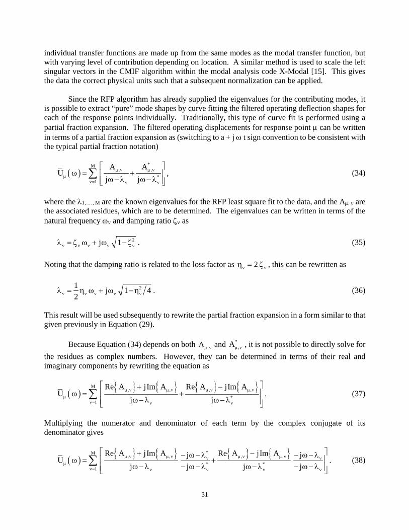
individual transfer functions are made up from the same modes as the modal transfer function, but with varying level of contribution depending on location. A similar method is used to scale the left singular vectors in the CMIF algorithm within the modal analysis code X-Modal [15]. This gives the data the correct physical units such that a subsequent normalization can be applied.

Since the RFP algorithm has already supplied the eigenvalues for the contributing modes, it is possible to extract “pure” mode shapes by curve fitting the filtered operating deflection shapes for each of the response points individually. Traditionally, this type of curve fit is performed using a partial fraction expansion. The filtered operating displacements for response point can be written in terms of a partial fraction expansion as (switching to a + j t sign convention to be consistent with the typical partial fraction notation)

*M

, ,

*1

A AU

j j

, (34)

wherethe 1, …, M are the known eigenvalues for the RFP least square fit to the data, and the A, are the associated residues, which are to be determined. The eigenvalues can be written in terms of the natural frequency and damping ratio as

2j 1 . (35)

Noting that the damping ratio is related to the loss factor as 2 , this can be rewritten as

21j 1 4

2 . (36)

This result will be used subsequently to rewrite the partial fraction expansion in a form similar to that given previously in Equation (29).

Because Equation (34) depends on both ,A and *,A , it is not possible to directly solve for

the residues as complex numbers. However, they can be determined in terms of their real and imaginary components by rewriting the equation as

M, , , ,

*1

Re A jIm A Re A jIm AU

j j

. (37)

Multiplying the numerator and denominator of each term by the complex conjugate of its denominator gives

*M, , , ,

* *1

Re A jIm A Re A jIm Aj jU

j j j j

. (38)

32

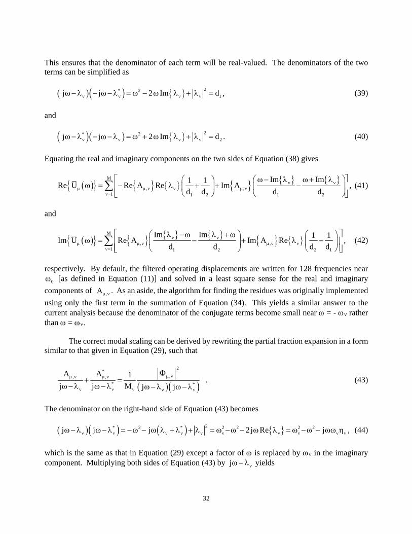
This ensures that the denominator of each term will be real-valued. The denominators of the two terms can be simplified as

2* 21j j 2 Im d , (39)

and

2* 22j j 2 Im d . (40)

Equating the real and imaginary components on the two sides of Equation (38) gives

M

, ,1 1 2 1 2

Im Im1 1Re U Re A Re Im A

d d d d

, (41)

and

M

, ,1 1 2 2 1

Im Im 1 1Im U Re A Im A Re

d d d d

, (42)

respectively. By default, the filtered operating displacements are written for 128 frequencies near

0 [as defined in Equation (11)] and solved in a least square sense for the real and imaginary

components of ,A . As an aside, the algorithm for finding the residues was originally implemented

using only the first term in the summation of Equation (34). This yields a similar answer to the current analysis because the denominator of the conjugate terms become small near = - rather than = . The correct modal scaling can be derived by rewriting the partial fraction expansion in a form similar to that given in Equation (29), such that

2*

,, ,

* *

A A 1

j j M j j

. (43)

The denominator on the right-hand side of Equation (43) becomes

2* 2 * 2 2 2 2j j j 2 j Re j , (44)

which is the same as that in Equation (29) except a factor of is replaced by in the imaginary component. Multiplying both sides of Equation (43) by j yields

33

2

,*, , * *

j 1A A

j M j

. (45)

Setting j then yields

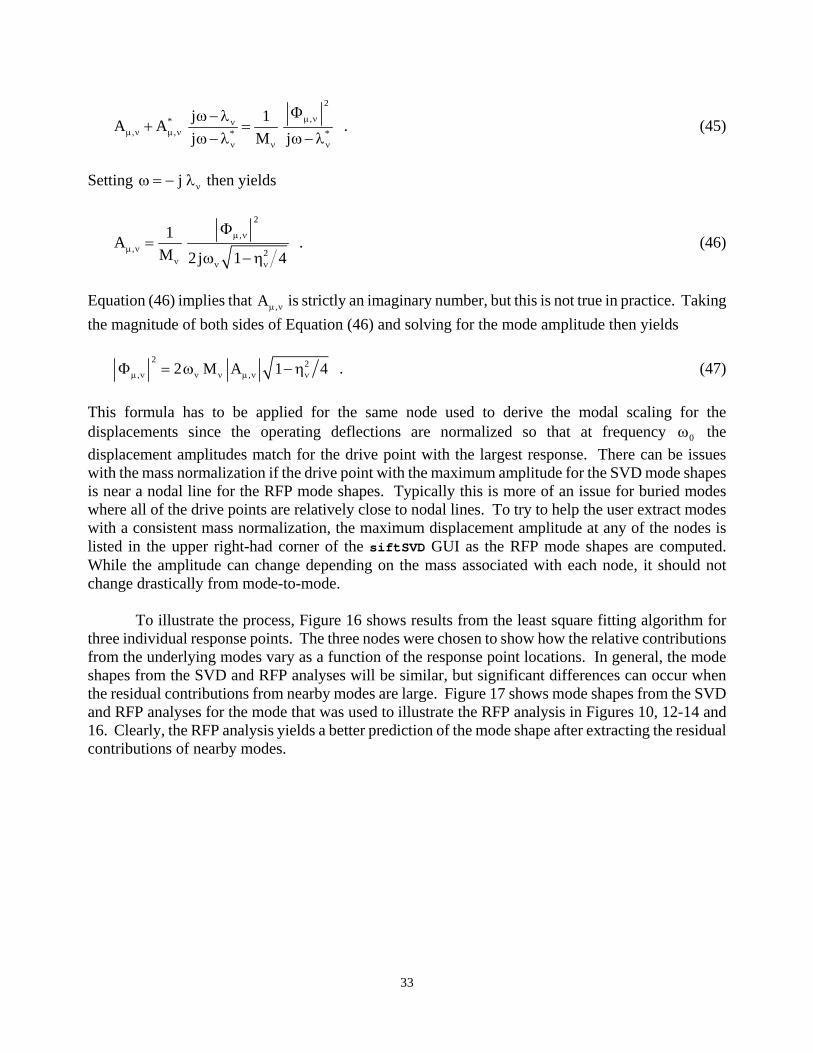
2

,

, 2

1A

M 2j 1 4

. (46)

Equation (46) implies that ,A is strictly an imaginary number, but this is not true in practice. Taking

the magnitude of both sides of Equation (46) and solving for the mode amplitude then yields

2 2

, ,2 M A 1 4 . (47)

This formula has to be applied for the same node used to derive the modal scaling for the displacements since the operating deflections are normalized so that at frequency 0 the

displacement amplitudes match for the drive point with the largest response. There can be issues with the mass normalization if the drive point with the maximum amplitude for the SVD mode shapes is near a nodal line for the RFP mode shapes. Typically this is more of an issue for buried modes where all of the drive points are relatively close to nodal lines. To try to help the user extract modes with a consistent mass normalization, the maximum displacement amplitude at any of the nodes is listed in the upper right-had corner of the siftSVD GUI as the RFP mode shapes are computed. While the amplitude can change depending on the mass associated with each node, it should not change drastically from mode-to-mode.

To illustrate the process, Figure 16 shows results from the least square fitting algorithm for three individual response points. The three nodes were chosen to show how the relative contributions from the underlying modes vary as a function of the response point locations. In general, the mode shapes from the SVD and RFP analyses will be similar, but significant differences can occur when the residual contributions from nearby modes are large. Figure 17 shows mode shapes from the SVD and RFP analyses for the mode that was used to illustrate the RFP analysis in Figures 10, 12-14 and 16. Clearly, the RFP analysis yields a better prediction of the mode shape after extracting the residual contributions of nearby modes.

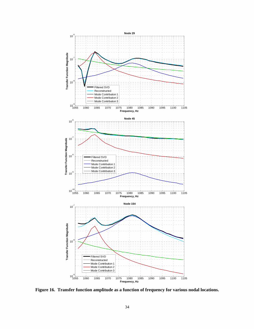
34

Figure 16. Transfer function amplitude as a function of frequency for various nodal locations.

1055 1060 1065 1070 1075 1080 1085 1090 1095 1100 110510

-9

10-8

10-7

10-6 Node 29

Frequency, Hz

Tra

ns

fer

Fu

nc

tio

n M

ag

nit

ud

e

Filtered SVDReconstructedMode Contribution 1Mode Contribution 2Mode Contribution 3

1055 1060 1065 1070 1075 1080 1085 1090 1095 1100 110510

-10

10-9

10-8

10-7

10-6 Node 45

Frequency, Hz

Tra

ns

fer

Fu

nc

tio

n M

ag

nit

ud

e

Filtered SVDReconstructedMode Contribution 1Mode Contribution 2Mode Contribution 3

1055 1060 1065 1070 1075 1080 1085 1090 1095 1100 110510

-9

10-8

10-7

Node 154

Frequency, Hz

Tra

ns

fer

Fu

nct

ion

Ma

gn

itu

de

Filtered SVDReconstructedMode Contribution 1Mode Contribution 2Mode Contribution 3

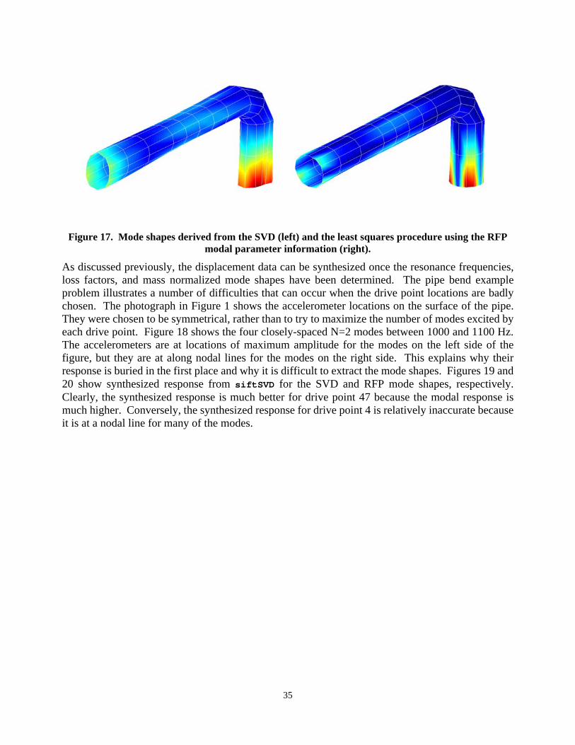
35

As discussed previously, the displacement data can be synthesized once the resonance frequencies, loss factors, and mass normalized mode shapes have been determined. The pipe bend example problem illustrates a number of difficulties that can occur when the drive point locations are badly chosen. The photograph in Figure 1 shows the accelerometer locations on the surface of the pipe. They were chosen to be symmetrical, rather than to try to maximize the number of modes excited by each drive point. Figure 18 shows the four closely-spaced N=2 modes between 1000 and 1100 Hz. The accelerometers are at locations of maximum amplitude for the modes on the left side of the figure, but they are at along nodal lines for the modes on the right side. This explains why their response is buried in the first place and why it is difficult to extract the mode shapes. Figures 19 and 20 show synthesized response from siftSVD for the SVD and RFP mode shapes, respectively. Clearly, the synthesized response is much better for drive point 47 because the modal response is much higher. Conversely, the synthesized response for drive point 4 is relatively inaccurate because it is at a nodal line for many of the modes.

Figure 17. Mode shapes derived from the SVD (left) and the least squares procedure using the RFP

modal parameter information (right).

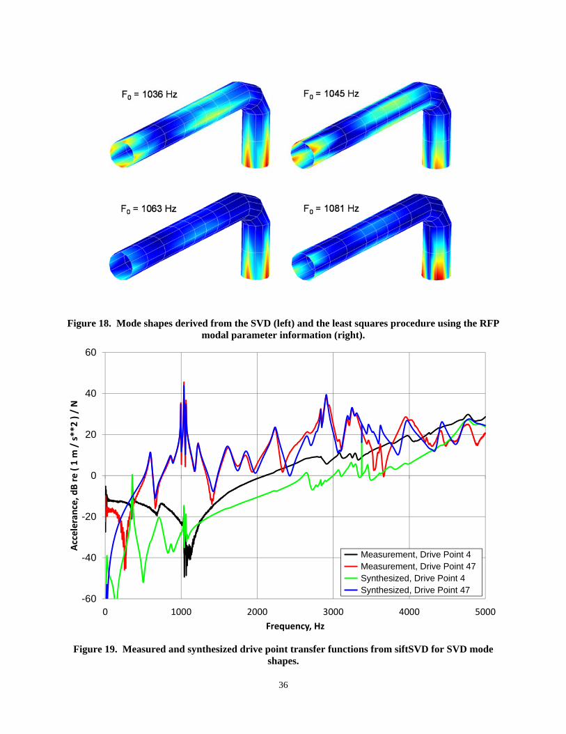
36

Figure 18. Mode shapes derived from the SVD (left) and the least squares procedure using the RFP

modal parameter information (right).

Figure 19. Measured and synthesized drive point transfer functions from siftSVD for SVD mode

shapes.

-60

-40

-20

0

20

40

60

0 1000 2000 3000 4000 5000

Acceleran

ce, d

B re ( 1 m

 / s**2 ) / N

Frequency, Hz

Measurement, Drive Point 4 Measurement, Drive Point 47 Synthesized, Drive Point 4 Synthesized, Drive Point 47

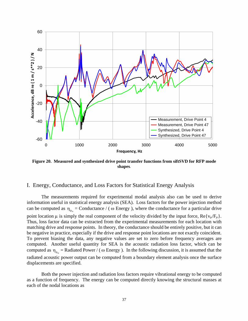
37

I. Energy, Conductance, and Loss Factors for Statistical Energy Analysis

The measurements required for experimental modal analysis also can be used to derive information useful in statistical energy analysis (SEA). Loss factors for the power injection method can be computed as

inp = Conductance / ( Energy ), where the conductance for a particular drive

point location is simply the real component of the velocity divided by the input force, Re{v/F}. Thus, loss factor data can be extracted from the experimental measurements for each location with matching drive and response points. In theory, the conductance should be entirely positive, but it can be negative in practice, especially if the drive and response point locations are not exactly coincident. To prevent biasing the data, any negative values are set to zero before frequency averages are computed. Another useful quantity for SEA is the acoustic radiation loss factor, which can be computed as

inp = Radiated Power / ( Energy ). In the following discussion, it is assumed that the

radiated acoustic power output can be computed from a boundary element analysis once the surface displacements are specified.

Both the power injection and radiation loss factors require vibrational energy to be computed

as a function of frequency. The energy can be computed directly knowing the structural masses at each of the nodal locations as

Figure 20. Measured and synthesized drive point transfer functions from siftSVD for RFP mode

shapes.

-60

-40

-20

0

20

40

60

0 1000 2000 3000 4000 5000

Accelerance, d

B re ( 1 m

 / s**2 ) / N

Frequency, Hz

Measurement, Drive Point 4 Measurement, Drive Point 47 Synthesized, Drive Point 4 Synthesized, Drive Point 47

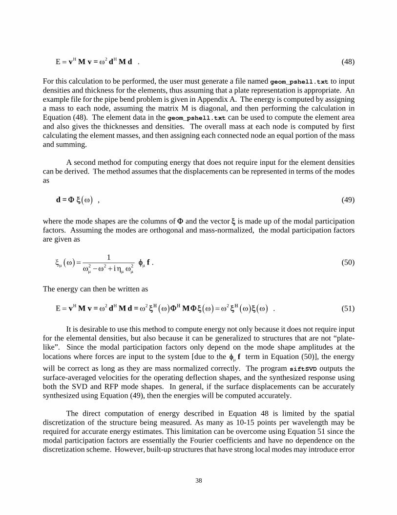
38

H 2 HE v M v = d M d . (48) For this calculation to be performed, the user must generate a file named geom_pshell.txt to input densities and thickness for the elements, thus assuming that a plate representation is appropriate. An example file for the pipe bend problem is given in Appendix A. The energy is computed by assigning a mass to each node, assuming the matrix M is diagonal, and then performing the calculation in Equation (48). The element data in the geom_pshell.txt can be used to compute the element area and also gives the thicknesses and densities. The overall mass at each node is computed by first calculating the element masses, and then assigning each connected node an equal portion of the mass and summing. A second method for computing energy that does not require input for the element densities can be derived. The method assumes that the displacements can be represented in terms of the modes as d = , (49)

where the mode shapes are the columns of and the vector is made up of the modal participation factors. Assuming the modes are orthogonal and mass-normalized, the modal participation factors are given as

2 2 2

1

if

. (50)

The energy can then be written as H 2 H 2 2E v M v = d M d = M . (51)

It is desirable to use this method to compute energy not only because it does not require input

for the elemental densities, but also because it can be generalized to structures that are not “plate-like”. Since the modal participation factors only depend on the mode shape amplitudes at the locations where forces are input to the system [due to the f term in Equation (50)], the energy

will be correct as long as they are mass normalized correctly. The program siftSVD outputs the surface-averaged velocities for the operating deflection shapes, and the synthesized response using both the SVD and RFP mode shapes. In general, if the surface displacements can be accurately synthesized using Equation (49), then the energies will be computed accurately.

The direct computation of energy described in Equation 48 is limited by the spatial discretization of the structure being measured. As many as 10-15 points per wavelength may be required for accurate energy estimates. This limitation can be overcome using Equation 51 since the modal participation factors are essentially the Fourier coefficients and have no dependence on the discretization scheme. However, built-up structures that have strong local modes may introduce error

39

into the estimates of the modal participation factor using Equation 51 and subsequently bias the energy estimates.

The boundary element program FORCE can be used to compute radiated acoustic sound power once the surface vibration profile over the boundary surface, i.e. the surface in contact with the fluid medium, is specified. The computations are typically performed for each measurement frequency and each drive point. Additionally, the data can be generated from the operating deflection shapes or synthesized data once the modes have been identified. The data for the analysis is written to a file named bc.txt by the programs MODAL_ANALYSIS_USING_SVD (for the operating deflection shapes) and siftSVD (for the synthesized response data). Thus, both programs should be run before performing the boundary element analysis. The boundary condition is written in the form of an elemental volume velocity distribution over the boundary surface in units of m3/s. The geom.txt file should be in the format listed in Appendix A.

In general, the source type (data field 8 for the element records) is not required when modal

analysis data is processed. However, it must be input correctly for the boundary element computations. In the NASTRAN format, data field 8 is a real number and this convention is followed for the geom.txt file to maintain compatibility with pre- and post-processors such as FEMAP. Briefly, the data field should be set to “0.” for plate elements in the plane of a baffle, “1.” for elements that are part of closed boundaries, and “2.” for surfaces represented by dipole sources (where both sides are in contact with the acoustic medium). More information for the acoustic boundary element analysis can be found in the book by Fahnline [16]. In addition to correctly formatting the geom.txt file, several parameters in the in.txt file must be set properly including CF which converts the nodal locations to meters, and IB indicating if the structure is baffled. The output from the analysis is written to a file named pow.txt for all the computations.

To try to simplify the analysis for the user, all of the boundary element computations are performed by executing the program FORCE once, and a second program named POST_PROCESS_EXPERIMENTAL_DATA is run after the computations are complete to rearrange the data, compute third octave averages, and write the output files. The results for the 1/3rd-octave averages are written to the files with “_OTO” included in the file name. The averages are computed by integrating over the frequency range of interest and then dividing the results by the bandwidth. The order of operations for these computations, as well as the OTO center, upper and lower frequencies, are listed in Appendix D. The post-processor relies on all of the data being in proper order in the pow.txt file and it also reads many of the other files generated by MODAL_ANALYSIS_USING_SVD and siftSVD. A run time error will thus be generated if the programs are not executed in the proper order or if any of the files are missing. A set of step-by-step instructions for performing a modal analysis and processing the data to produce information used in SEA is given in Appendix B and descriptions of all the output files are given in Appendix C.

J. Summary and Future Work This report documents ARL’s procedure for performing experimental modal analysis. The basic numerical techniques follow those developed at the University of Cincinnati for Complex Mode

40

Indicator Functions, although many of the implementation details are different. The analysis is designed primarily for experimental datasets with multiple drive and response points and has proven effective even for systems with numerous closely spaced resonance frequencies and relatively high noise levels. The report also documents the use of the graphical interface for eliminating misidentified modes and refining the resonance frequency and loss factor predictions. An example problem of a pipe with a bend is given to demonstrate the accuracy of the calculations and the expected results.

REFERENCES 1 D. J. Ewins, Modal Testing: Theory, Practice, and Applications, 2nd Ed., (Research Studies Press,

Hertfordshire, England, 2001). 2 S. Maia, J. M. M. Silva, J. He, N. A. Lieven, R. M. Lin, G. W. Skingle, W. M. To, and A. P. V.

Urgueira, Theoretical and Experimental Modal Analysis, (Research Studies Press, Hertfordshire, England, 1997).

3 R. J. Allemang and D. L .Brown, “Experimental Modal Analysis,” Handbook on Experimental

Mechanics, 2nd Revised Ed., pp. 635-750, 1993. 4 D. Formenti and M. Richardson, "Parameter estimation from frequency response measurements

using rational fraction polynomials (twenty years of progress)," in Proceedings of the Twentieth International Modal Analysis Conference, pp. 373-382, 2002.

5 C. Y. Shih, Y. G. Tsuei, R. J. Allemang, and D. L. Brown, "Complex mode indication function and

its applications to spacial domain parameter estimation," in Proceedings of the Seventh International Modal Analysis Conference, pp. 533-540, 1989.

6 A. W. Phillips, R. J. Allemang, and W. A. Fladung, "The complex mode indication function (CMIF)

as a parameter estimation method," in Proceedings of the Sixteenth International Modal Analysis Conference, pp. 705-710, 1998.

7 S. Li, W. A. Fladung, W. A. Phillips, and D. L. Brown, "Automotive applications of the enhanced

mode indicator function parameter estimation method," in Proceedings of the Sixteenth International Modal Analysis Conference, pp. 36-44, 1998.

8 F. Necati Catbas, D. L. Brown, A. Emin Aktan, “Parameter estimation for multiple-input multiple-

output modal analysis of large structures”, J. Eng. Mech., 130 (8), 921-930, 2004. 9 R. J. Allemang, Vibrations: Experimental Modal Analysis, UC-SDRL-CN-20-263-663/664,

(University of Cincinnati, Cincinnati, OH, 2007). 10 J. P. Caffrey and J. M. Lee, MSC/NASTRAN User’s Guide: Linear Static Analysis, (Macneal-

Schwendler Corp., Los Angeles, CA, 1994), pp 489-493.

41

11 A. V. Oppenheim and R. W. Schaffer, Discrete-Time Signal Processing, (Prentice-Hall, Englewood Cliffs, NJ, 1989), pp. 514-517.

12 W. H. Press, S. A. Teukolsky, W. T. Vetterling, and B. P. Flannery, Numerical Recipes in

FORTRAN, (Cambridge University Press, Cambridge, 1992), pp. 644-649. 13 J. M. Montalvao, E Silva and N. M. M. Maia, "Single mode identification techniques for use with

small microcomputers," in J. Sound. Vib., pp. 13-26, 1988. 14 A. M. Iglesias, Investigating Various Modal Analysis Techniques to Estimate Damping Ratio,

Master’s Thesis, (Virginia Polytechnic Institute and State University, Blacksburg, VA, 2000). 15 Experimental Modal Analysis, UC-SDRL Experimental Techniques Seminar Series, Lecture

Notes – Part 1, (University of Cincinnati, Cincinnati, OH, 2009), pg 8-13. 16 J. B. Fahnline, Numerically Computing the Acoustic Power Output of a Vibrating Structure Using

a Lumped Parameter Model, (Unpublished), pp. 24-27.

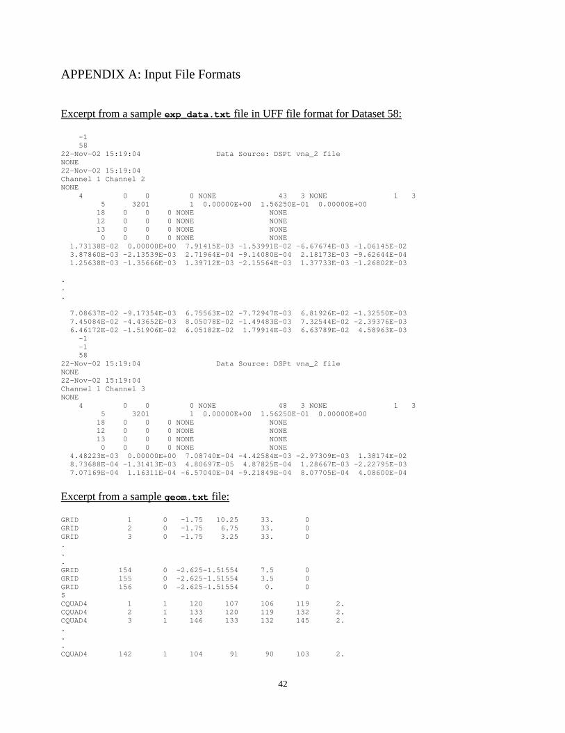
42

APPENDIX A: Input File Formats Excerpt from a sample exp_data.txt file in UFF file format for Dataset 58: -1 58 22-Nov-02 15:19:04 Data Source: DSPt vna_2 file NONE 22-Nov-02 15:19:04 Channel 1 Channel 2 NONE 4 0 0 0 NONE 43 3 NONE 1 3 5 3201 1 0.00000E+00 1.56250E-01 0.00000E+00 18 0 0 0 NONE NONE 12 0 0 0 NONE NONE 13 0 0 0 NONE NONE 0 0 0 0 NONE NONE 1.73138E-02 0.00000E+00 7.91415E-03 -1.53991E-02 -6.67674E-03 -1.06145E-02 3.87860E-03 -2.13539E-03 2.71964E-04 -9.14080E-04 2.18173E-03 -9.62644E-04 1.25638E-03 -1.35666E-03 1.39712E-03 -2.15564E-03 1.37733E-03 -1.26802E-03 . . . 7.08637E-02 -9.17354E-03 6.75563E-02 -7.72947E-03 6.81926E-02 -1.32550E-03 7.45084E-02 -4.43652E-03 8.05078E-02 -1.49483E-03 7.32544E-02 -2.39376E-03 6.46172E-02 -1.51906E-02 6.05182E-02 1.79914E-03 6.63789E-02 4.58963E-03 -1 -1 58 22-Nov-02 15:19:04 Data Source: DSPt vna_2 file NONE 22-Nov-02 15:19:04 Channel 1 Channel 3 NONE 4 0 0 0 NONE 48 3 NONE 1 3 5 3201 1 0.00000E+00 1.56250E-01 0.00000E+00 18 0 0 0 NONE NONE 12 0 0 0 NONE NONE 13 0 0 0 NONE NONE 0 0 0 0 NONE NONE 4.48223E-03 0.00000E+00 7.08740E-04 -4.42584E-03 -2.97309E-03 1.38174E-02 8.73688E-04 -1.31413E-03 4.80697E-05 4.87825E-04 1.28667E-03 -2.22795E-03 7.07169E-04 1.16311E-04 -6.57040E-04 -9.21849E-04 8.07705E-04 4.08600E-04

Excerpt from a sample geom.txt file: GRID 1 0 -1.75 10.25 33. 0 GRID 2 0 -1.75 6.75 33. 0 GRID 3 0 -1.75 3.25 33. 0 . . . GRID 154 0 -2.625-1.51554 7.5 0 GRID 155 0 -2.625-1.51554 3.5 0 GRID 156 0 -2.625-1.51554 0. 0 $ CQUAD4 1 1 120 107 106 119 2. CQUAD4 2 1 133 120 119 132 2. CQUAD4 3 1 146 133 132 145 2. . . . CQUAD4 142 1 104 91 90 103 2.

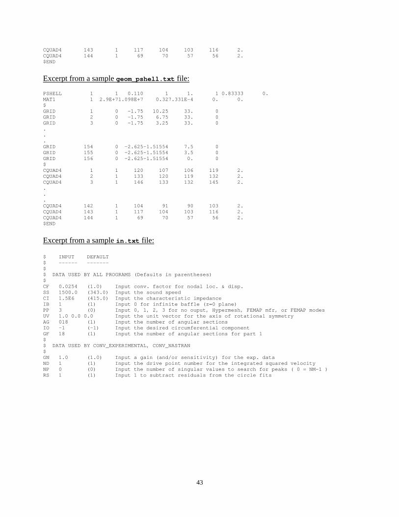
43

CQUAD4 143 1 117 104 103 116 2. CQUAD4 144 1 69 70 57 56 2. $END Excerpt from a sample geom_pshell.txt file: PSHELL 1 1 0.110 1 1. 1 0.83333 0. MAT1 1 2.9E+71.098E+7 0.327.331E-4 0. 0. $ GRID 1 0 -1.75 10.25 33. 0 GRID 2 0 -1.75 6.75 33. 0 GRID 3 0 -1.75 3.25 33. 0 . . . GRID 154 0 -2.625-1.51554 7.5 0 GRID 155 0 -2.625-1.51554 3.5 0 GRID 156 0 -2.625-1.51554 0. 0 $ CQUAD4 1 1 120 107 106 119 2. CQUAD4 2 1 133 120 119 132 2. CQUAD4 3 1 146 133 132 145 2. . . . CQUAD4 142 1 104 91 90 103 2. CQUAD4 143 1 117 104 103 116 2. CQUAD4 144 1 69 70 57 56 2. $END

Excerpt from a sample in.txt file: $ INPUT DEFAULT $ ------ ------- $ $ DATA USED BY ALL PROGRAMS (Defaults in parentheses) $ CF 0.0254 (1.0) Input conv. factor for nodal loc. & disp. SS 1500.0 (343.0) Input the sound speed CI 1.5E6 (415.0) Input the characteristic impedance IB 1 (1) Input 0 for infinite baffle (z=0 plane) PP 3 (0) Input 0, 1, 2, 3 for no ouput, Hypermesh, FEMAP mfr, or FEMAP modes UV 1.0 0.0 0.0 Input the unit vector for the axis of rotational symmetry AG 018 (1) Input the number of angular sections IO -1 (-1) Input the desired circumferential component GF 18 (1) Input the number of angular sections for part 1 $ $ DATA USED BY CONV_EXPERIMENTAL, CONV_NASTRAN $ GN 1.0 (1.0) Input a gain (and/or sensitivity) for the exp. data ND 1 (1) Input the drive point number for the integrated squared velocity NP 0 (0) Input the number of singular values to search for peaks ( 0 = NM-1 ) RS 1 (1) Input 1 to subtract residuals from the circle fits

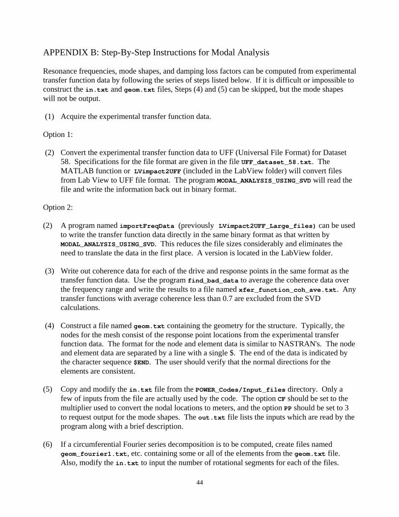
44

APPENDIX B: Step-By-Step Instructions for Modal Analysis Resonance frequencies, mode shapes, and damping loss factors can be computed from experimental transfer function data by following the series of steps listed below. If it is difficult or impossible to construct the in.txt and geom.txt files, Steps (4) and (5) can be skipped, but the mode shapes will not be output. (1) Acquire the experimental transfer function data. Option 1: (2) Convert the experimental transfer function data to UFF (Universal File Format) for Dataset

58. Specifications for the file format are given in the file UFF_dataset_58.txt. The MATLAB function or LVimpact2UFF (included in the LabView folder) will convert files from Lab View to UFF file format. The program MODAL_ANALYSIS_USING_SVD will read the file and write the information back out in binary format.

Option 2: (2) A program named importFreqData (previously LVimpact2UFF_Large_files) can be used

to write the transfer function data directly in the same binary format as that written by MODAL_ANALYSIS_USING_SVD. This reduces the file sizes considerably and eliminates the need to translate the data in the first place. A version is located in the LabView folder.

(3) Write out coherence data for each of the drive and response points in the same format as the

transfer function data. Use the program find_bad_data to average the coherence data over the frequency range and write the results to a file named xfer_function_coh_ave.txt. Any transfer functions with average coherence less than 0.7 are excluded from the SVD calculations.

(4) Construct a file named geom.txt containing the geometry for the structure. Typically, the

nodes for the mesh consist of the response point locations from the experimental transfer function data. The format for the node and element data is similar to NASTRAN's. The node and element data are separated by a line with a single $. The end of the data is indicated by the character sequence $END. The user should verify that the normal directions for the elements are consistent.

(5) Copy and modify the in.txt file from the POWER_Codes/Input_files directory. Only a

few of inputs from the file are actually used by the code. The option CF should be set to the multiplier used to convert the nodal locations to meters, and the option PP should be set to 3 to request output for the mode shapes. The out.txt file lists the inputs which are read by the program along with a brief description.

(6) If a circumferential Fourier series decomposition is to be computed, create files named

geom_fourier1.txt, etc. containing some or all of the elements from the geom.txt file. Also, modify the in.txt to input the number of rotational segments for each of the files.

45

(7) If energies are to be computed, create a file named geom_pshell.txt with the correct

materials and properties for the element mesh. (8) Place the MODAL_ANALYSIS_USING_SVD.exe in the same folder with the other files and

execute the program. This can be done by “double-clicking” on the executable or typing ./MODAL_ANALYSIS_USING_SVD.exe from within Cygwin after navigating to the working directory. If an error occurs, an explanation of the problem is typically written to the file out.txt. Run time errors are often easier to diagnose in Cygwin because the execution window closes too fast to read the error messages otherwise.

(9) After the program is finished, start MATLAB, change to the working directory, and execute

the program siftSVD (Y:\Common\Noise Control and Acoustic Division\Structural Acoustics Department\Matlab\FE_BETools). The listed folder must be in your path or else the command will not execute. Choose to keep or reject modes by picking the yes or no buttons with the mouse by typing "y" or "n", respectively. Also, if you make a mistake you can go back by picking the “back” button with the mouse or typing "b". If you pick the “stop” button with the mouse or type "s", the program skips over the rest of the modes and rearranges the data for the modes already chosen. By default, the RFP order is set to 1. A different order can be chosen by typing a number and picking the desired transfer function from among the dashed curves. To view mode shape animations while analyzing the data, create a geom_animate.txt file, which is the same as geom.txt unless there are multiple response data at a single point (due to different directions). A more detailed description of the process of using the RFP interface can be found in the User’s Guide.

(10) If a boundary element analysis is to be performed, copy the file FORCE.exe to the working

directory. The geom.txt file needs to include source type information and the parameter CF used to convert the nodal locations to meters must be set properly in the in.txt file.

(11) Finally, the program POST_PROCESS_EXPERIMENTAL_DATA.exe can be used to compute

power injection quantities, radiation loss factors, and to rearrange the power output data in the pow.txt file. One-third octave band averages are also computed and output. Descriptions of the results can be found in the readme.txt file.

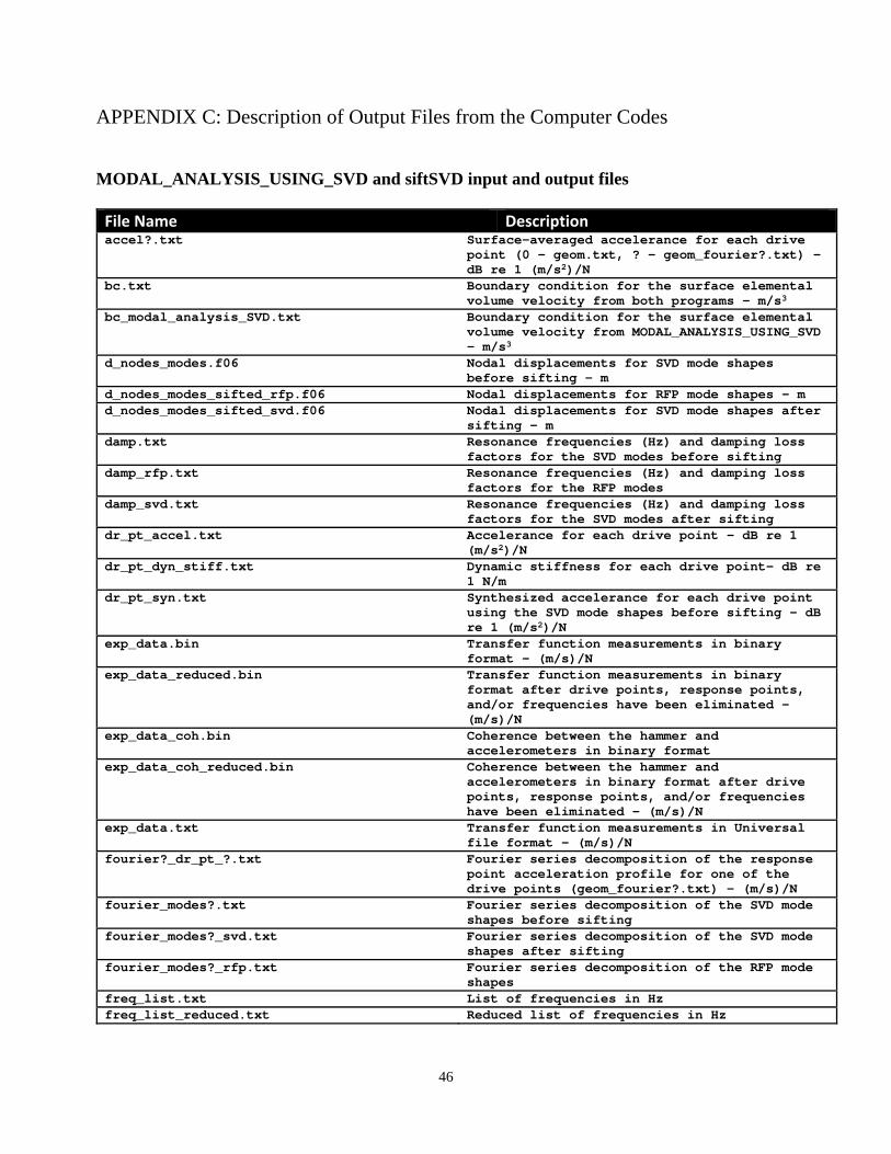
46

APPENDIX C: Description of Output Files from the Computer Codes MODAL_ANALYSIS_USING_SVD and siftSVD input and output files File Name  Description accel?.txt Surface-averaged accelerance for each drive

point (0 – geom.txt, ? - geom_fourier?.txt) – dB re 1 (m/s2)/N

bc.txt Boundary condition for the surface elemental volume velocity from both programs – m/s3

bc_modal_analysis_SVD.txt Boundary condition for the surface elemental volume velocity from MODAL_ANALYSIS_USING_SVD – m/s3

d_nodes_modes.f06 Nodal displacements for SVD mode shapes before sifting - m

d_nodes_modes_sifted_rfp.f06 Nodal displacements for RFP mode shapes - md_nodes_modes_sifted_svd.f06 Nodal displacements for SVD mode shapes after

sifting - m damp.txt Resonance frequencies (Hz) and damping loss

factors for the SVD modes before sifting damp_rfp.txt Resonance frequencies (Hz) and damping loss

factors for the RFP modes damp_svd.txt Resonance frequencies (Hz) and damping loss

factors for the SVD modes after sifting dr_pt_accel.txt Accelerance for each drive point – dB re 1

(m/s2)/N dr_pt_dyn_stiff.txt Dynamic stiffness for each drive point– dB re

1 N/m dr_pt_syn.txt Synthesized accelerance for each drive point

using the SVD mode shapes before sifting – dB re 1 (m/s2)/N

exp_data.bin Transfer function measurements in binary format – (m/s)/N

exp_data_reduced.bin Transfer function measurements in binary format after drive points, response points, and/or frequencies have been eliminated – (m/s)/N

exp_data_coh.bin Coherence between the hammer and accelerometers in binary format

exp_data_coh_reduced.bin Coherence between the hammer and accelerometers in binary format after drive points, response points, and/or frequencies have been eliminated – (m/s)/N

exp_data.txt Transfer function measurements in Universal file format – (m/s)/N

fourier?_dr_pt_?.txt Fourier series decomposition of the response point acceleration profile for one of the drive points (geom_fourier?.txt) – (m/s)/N

fourier_modes?.txt Fourier series decomposition of the SVD mode shapes before sifting

fourier_modes?_svd.txt Fourier series decomposition of the SVD mode shapes after sifting

fourier_modes?_rfp.txt Fourier series decomposition of the RFP mode shapes

freq_list.txt List of frequencies in Hz freq_list_reduced.txt Reduced list of frequencies in Hz

47

geom.txt The surface element mesh made up of 3-noded triangular and 4-noded quadrilateral elements in NASTRAN format

geom_animate.txt The element mesh in NASTRAN format for the animation, which can include other element types such as beam and bar elements

geom_fourier?.txt A surface element mesh for the Fourier series decomposition composed of elements from geom.txt file with the same element numbers

geom_pshell.txt The same surface element mesh in the geom.txt file with the element properties and materials used input to compute nodal masses

in.txt A file containing the input parameters for the computer codes written in FORTRAN by John Fahnline

node_list_drive.txt The list of drive points in the experimental transfer function data

node_list_drive_reduced.txt A user-created list of drive points with 0’s replacing the points to be eliminated

node_list_drive_reduced_wo_zeros.txt A reduced list of drive points node_list_resp.txt The list of response points in the

experimental transfer function data node_list_resp_reduced.txt A user-created list of response points with

0’s replacing the points to be eliminated node_list_resp_reduced_wo_zeros.txt A reduced list of response points ods_damp_pin.txt Power injection damping loss factors for the

operating deflection shapes ods_damp_pin_OTO.txt Power injection damping loss factors for the

operating deflection shapes in 1/3-octave bands

ods_damp_prad.txt Acoustic radiation damping loss factors for the operating deflection shapes

ods_damp_prad_OTO.txt Acoustic radiation damping loss factors for the operating deflection shapes in 1/3-octave bands

ods_dr_pt_conductance.txt Drive point conductance (real part of mobility) for the operating deflection shapes – (m/s)/N

ods_dr_pt_conductance_OTO.txt Drive point conductance (real part of mobility) for the operating deflection shapes in 1/3-octave bands – (m/s)/N

ods_energy.txt Energy for the operating deflection shapes as output from MODAL_ANALYSIS_USING_SVD by assuming the mass is concentrated at the nodes

ods_energy_point_average_pshell.txt Energy for the operating deflection shapes as output from siftSVD by assuming the mass is concentrated at the nodes

ods_energy_point_average_pshell_OTO.txt Energy for the operating deflection shapes as output from siftSVD by assuming the mass is concentrated at the nodes in 1/3-octave bands

ods_high.txt Squared normal velocity integrated over the surface mesh from the geom.txt file for the operating deflection shapes – dB re 1x10-12 Watts

ods_power.txt Acoustic power output for the operating deflection shapes – dB re 1x10-12 Watts

ods_power_OTO.txt Acoustic power output for the operating deflection shapes in 1/3-octave bands – dB re 1x10-12 Watts

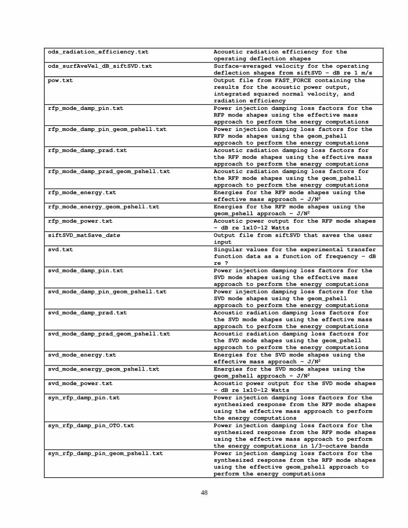
48

ods_radiation_efficiency.txt Acoustic radiation efficiency for the operating deflection shapes

ods_surfAveVel_dB_siftSVD.txt Surface-averaged velocity for the operating deflection shapes from siftSVD – dB re 1 m/s

pow.txt Output file from FAST_FORCE containing the results for the acoustic power output, integrated squared normal velocity, and radiation efficiency

rfp_mode_damp_pin.txt Power injection damping loss factors for the RFP mode shapes using the effective mass approach to perform the energy computations

rfp_mode_damp_pin_geom_pshell.txt Power injection damping loss factors for the RFP mode shapes using the geom_pshell approach to perform the energy computations

rfp_mode_damp_prad.txt Acoustic radiation damping loss factors for the RFP mode shapes using the effective mass approach to perform the energy computations

rfp_mode_damp_prad_geom_pshell.txt Acoustic radiation damping loss factors for the RFP mode shapes using the geom_pshell approach to perform the energy computations

rfp_mode_energy.txt Energies for the RFP mode shapes using the effective mass approach – J/N2

rfp_mode_energy_geom_pshell.txt Energies for the RFP mode shapes using the geom_pshell approach – J/N2

rfp_mode_power.txt Acoustic power output for the RFP mode shapes - dB re 1x10-12 Watts

siftSVD_matSave_date Output file from siftSVD that saves the user input

svd.txt Singular values for the experimental transfer function data as a function of frequency – dB re ?

svd_mode_damp_pin.txt Power injection damping loss factors for the SVD mode shapes using the effective mass approach to perform the energy computations

svd_mode_damp_pin_geom_pshell.txt Power injection damping loss factors for the SVD mode shapes using the geom_pshell approach to perform the energy computations

svd_mode_damp_prad.txt Acoustic radiation damping loss factors for the SVD mode shapes using the effective mass approach to perform the energy computations

svd_mode_damp_prad_geom_pshell.txt Acoustic radiation damping loss factors for the SVD mode shapes using the geom_pshell approach to perform the energy computations

svd_mode_energy.txt Energies for the SVD mode shapes using the effective mass approach – J/N2

svd_mode_energy_geom_pshell.txt Energies for the SVD mode shapes using the geom_pshell approach – J/N2

svd_mode_power.txt Acoustic power output for the SVD mode shapes - dB re 1x10-12 Watts

syn_rfp_damp_pin.txt Power injection damping loss factors for the synthesized response from the RFP mode shapes using the effective mass approach to perform the energy computations

syn_rfp_damp_pin_OTO.txt Power injection damping loss factors for the synthesized response from the RFP mode shapes using the effective mass approach to perform the energy computations in 1/3-octave bands

syn_rfp_damp_pin_geom_pshell.txt Power injection damping loss factors for the synthesized response from the RFP mode shapes using the effective geom_pshell approach to perform the energy computations

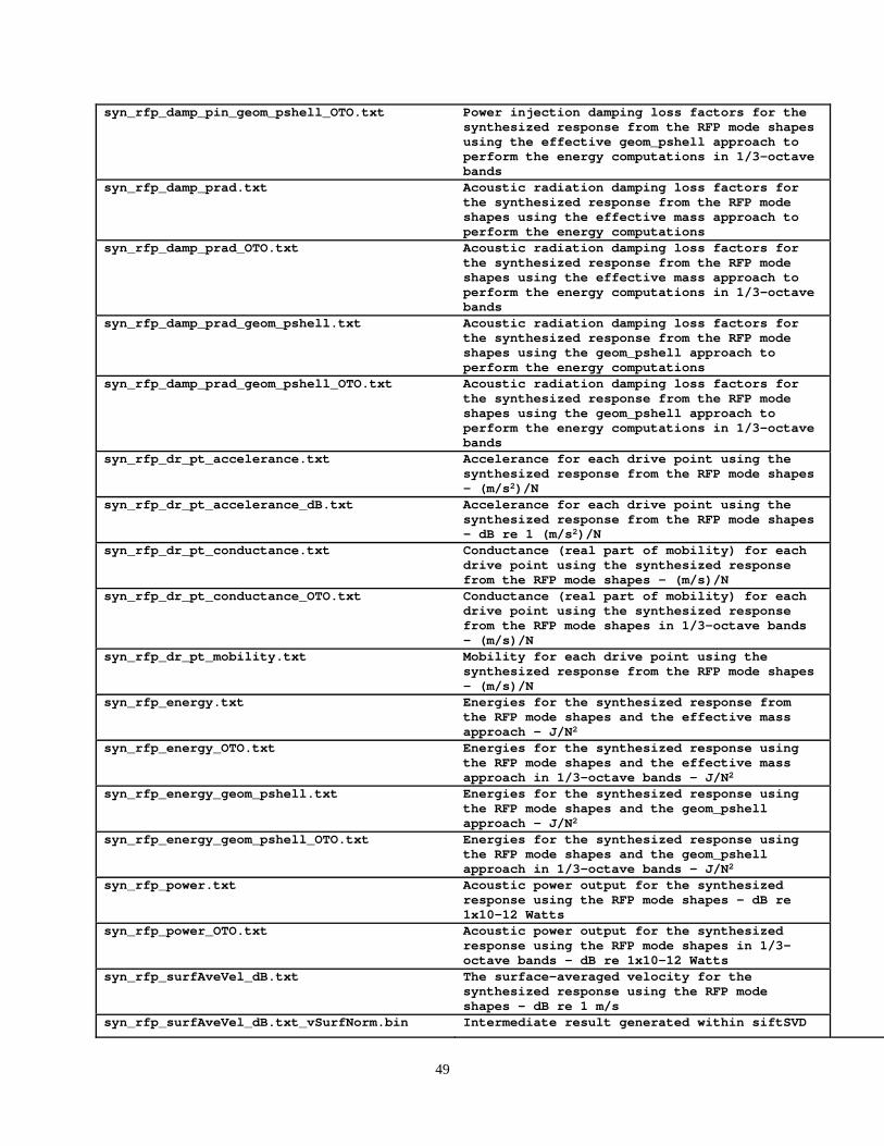
49

syn_rfp_damp_pin_geom_pshell_OTO.txt Power injection damping loss factors for the synthesized response from the RFP mode shapes using the effective geom_pshell approach to perform the energy computations in 1/3-octave bands

syn_rfp_damp_prad.txt Acoustic radiation damping loss factors for the synthesized response from the RFP mode shapes using the effective mass approach to perform the energy computations

syn_rfp_damp_prad_OTO.txt Acoustic radiation damping loss factors for the synthesized response from the RFP mode shapes using the effective mass approach to perform the energy computations in 1/3-octave bands

syn_rfp_damp_prad_geom_pshell.txt Acoustic radiation damping loss factors for the synthesized response from the RFP mode shapes using the geom_pshell approach to perform the energy computations

syn_rfp_damp_prad_geom_pshell_OTO.txt Acoustic radiation damping loss factors for the synthesized response from the RFP mode shapes using the geom_pshell approach to perform the energy computations in 1/3-octave bands

syn_rfp_dr_pt_accelerance.txt Accelerance for each drive point using the synthesized response from the RFP mode shapes – (m/s2)/N

syn_rfp_dr_pt_accelerance_dB.txt Accelerance for each drive point using the synthesized response from the RFP mode shapes – dB re 1 (m/s2)/N

syn_rfp_dr_pt_conductance.txt Conductance (real part of mobility) for each drive point using the synthesized response from the RFP mode shapes – (m/s)/N

syn_rfp_dr_pt_conductance_OTO.txt Conductance (real part of mobility) for each drive point using the synthesized response from the RFP mode shapes in 1/3-octave bands – (m/s)/N

syn_rfp_dr_pt_mobility.txt Mobility for each drive point using the synthesized response from the RFP mode shapes – (m/s)/N

syn_rfp_energy.txt Energies for the synthesized response from the RFP mode shapes and the effective mass approach – J/N2

syn_rfp_energy_OTO.txt Energies for the synthesized response using the RFP mode shapes and the effective mass approach in 1/3-octave bands – J/N2

syn_rfp_energy_geom_pshell.txt Energies for the synthesized response using the RFP mode shapes and the geom_pshell approach – J/N2

syn_rfp_energy_geom_pshell_OTO.txt Energies for the synthesized response using the RFP mode shapes and the geom_pshell approach in 1/3-octave bands – J/N2

syn_rfp_power.txt Acoustic power output for the synthesized response using the RFP mode shapes - dB re 1x10-12 Watts

 

syn_rfp_power_OTO.txt Acoustic power output for the synthesized response using the RFP mode shapes in 1/3-octave bands - dB re 1x10-12 Watts

 

syn_rfp_surfAveVel_dB.txt The surface-averaged velocity for the synthesized response using the RFP mode shapes – dB re 1 m/s

 

syn_rfp_surfAveVel_dB.txt_vSurfNorm.bin Intermediate result generated within siftSVD  

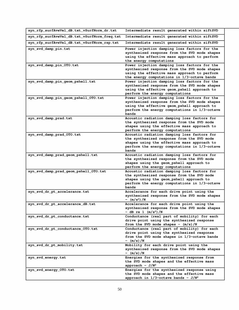
50

syn_rfp_surfAveVel_dB.txt_vSurfNorm_dr.txt Intermediate result generated within siftSVD  syn_rfp_surfAveVel_dB.txt_vSurfNorm_freq.txt Intermediate result generated within siftSVD  syn_rfp_surfAveVel_dB.txt_vSurfNorm_rsp.txt Intermediate result generated within siftSVD  syn_svd_damp_pin.txt Power injection damping loss factors for the

synthesized response from the SVD mode shapes using the effective mass approach to perform the energy computations

syn_svd_damp_pin_OTO.txt Power injection damping loss factors for the synthesized response from the SVD mode shapes using the effective mass approach to perform the energy computations in 1/3-octave bands

syn_svd_damp_pin_geom_pshell.txt Power injection damping loss factors for the synthesized response from the SVD mode shapes using the effective geom_pshell approach to perform the energy computations

syn_svd_damp_pin_geom_pshell_OTO.txt Power injection damping loss factors for the synthesized response from the SVD mode shapes using the effective geom_pshell approach to perform the energy computations in 1/3-octave bands

syn_svd_damp_prad.txt Acoustic radiation damping loss factors for the synthesized response from the SVD mode shapes using the effective mass approach to perform the energy computations

syn_svd_damp_prad_OTO.txt Acoustic radiation damping loss factors for the synthesized response from the SVD mode shapes using the effective mass approach to perform the energy computations in 1/3-octave bands

syn_svd_damp_prad_geom_pshell.txt Acoustic radiation damping loss factors for the synthesized response from the SVD mode shapes using the geom_pshell approach to perform the energy computations

syn_svd_damp_prad_geom_pshell_OTO.txt Acoustic radiation damping loss factors for the synthesized response from the SVD mode shapes using the geom_pshell approach to perform the energy computations in 1/3-octave bands

syn_svd_dr_pt_accelerance.txt Accelerance for each drive point using the synthesized response from the SVD mode shapes – (m/s2)/N

syn_svd_dr_pt_accelerance_dB.txt Accelerance for each drive point using the synthesized response from the SVD mode shapes – dB re 1 (m/s2)/N

syn_svd_dr_pt_conductance.txt Conductance (real part of mobility) for each drive point using the synthesized response from the SVD mode shapes – (m/s)/N

syn_svd_dr_pt_conductance_OTO.txt Conductance (real part of mobility) for each drive point using the synthesized response from the SVD mode shapes in 1/3-octave bands – (m/s)/N

syn_svd_dr_pt_mobility.txt Mobility for each drive point using the synthesized response from the SVD mode shapes – (m/s)/N

syn_svd_energy.txt Energies for the synthesized response from the SVD mode shapes and the effective mass approach – J/N2

syn_svd_energy_OTO.txt Energies for the synthesized response using the SVD mode shapes and the effective mass approach in 1/3-octave bands – J/N2

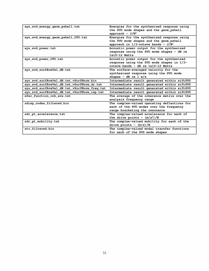
51

syn_svd_energy_geom_pshell.txt Energies for the synthesized response using the SVD mode shapes and the geom_pshell approach – J/N2

syn_svd_energy_geom_pshell_OTO.txt Energies for the synthesized response using the SVD mode shapes and the geom_pshell approach in 1/3-octave bands – J/N2

syn_svd_power.txt Acoustic power output for the synthesized response using the SVD mode shapes - dB re 1x10-12 Watts

syn_svd_power_OTO.txt Acoustic power output for the synthesized response using the SVD mode shapes in 1/3-octave bands - dB re 1x10-12 Watts

syn_svd_surfAveVel_dB.txt The surface-averaged velocity for the synthesized response using the SVD mode shapes – dB re 1 m/s

syn_svd_surfAveVel_dB.txt_vSurfNorm.bin Intermediate result generated within siftSVD syn_svd_surfAveVel_dB.txt_vSurfNorm_dr.txt Intermediate result generated within siftSVDsyn_svd_surfAveVel_dB.txt_vSurfNorm_freq.txt Intermediate result generated within siftSVDsyn_svd_surfAveVel_dB.txt_vSurfNorm_rsp.txt Intermediate result generated within siftSVDxfer_function_coh_ave.txt The average of the coherence matrix over the

analysis frequency range zdisp_nodes_filtered.bin The complex-valued operating deflections for

each of the SVD modes over the frequency range bracketing the resonance

zdr_pt_accelerance.txt The complex-valued accelerance for each of the drive points - (m/s2)/N

zdr_pt_mobility.txt The complex-valued mobility for each of the drive points - (m/s)/N

ztr_filtered.bin The complex-valued modal transfer functions for each of the SVD mode shapes

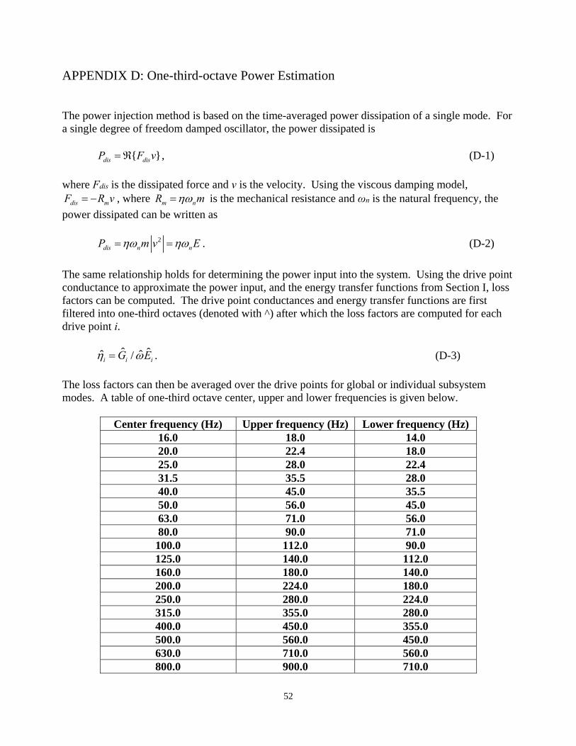
52

APPENDIX D: One-third-octave Power Estimation The power injection method is based on the time-averaged power dissipation of a single mode. For a single degree of freedom damped oscillator, the power dissipated is

{ }dis disP F v , (D-1)

where Fdis is the dissipated force and v is the velocity. Using the viscous damping model,

dis mF R v , where m nR m is the mechanical resistance and ωn is the natural frequency, the

power dissipated can be written as

2dis n nP m v E . (D-2)

The same relationship holds for determining the power input into the system. Using the drive point conductance to approximate the power input, and the energy transfer functions from Section I, loss factors can be computed. The drive point conductances and energy transfer functions are first filtered into one-third octaves (denoted with ^) after which the loss factors are computed for each drive point i.

ˆ ˆˆ ˆ/i i iG E . (D-3)

The loss factors can then be averaged over the drive points for global or individual subsystem modes. A table of one-third octave center, upper and lower frequencies is given below.

Center frequency (Hz) Upper frequency (Hz) Lower frequency (Hz)

16.0 18.0 14.0 20.0 22.4 18.0 25.0 28.0 22.4 31.5 35.5 28.0 40.0 45.0 35.5 50.0 56.0 45.0 63.0 71.0 56.0 80.0 90.0 71.0 100.0 112.0 90.0 125.0 140.0 112.0 160.0 180.0 140.0 200.0 224.0 180.0 250.0 280.0 224.0 315.0 355.0 280.0 400.0 450.0 355.0 500.0 560.0 450.0 630.0 710.0 560.0 800.0 900.0 710.0

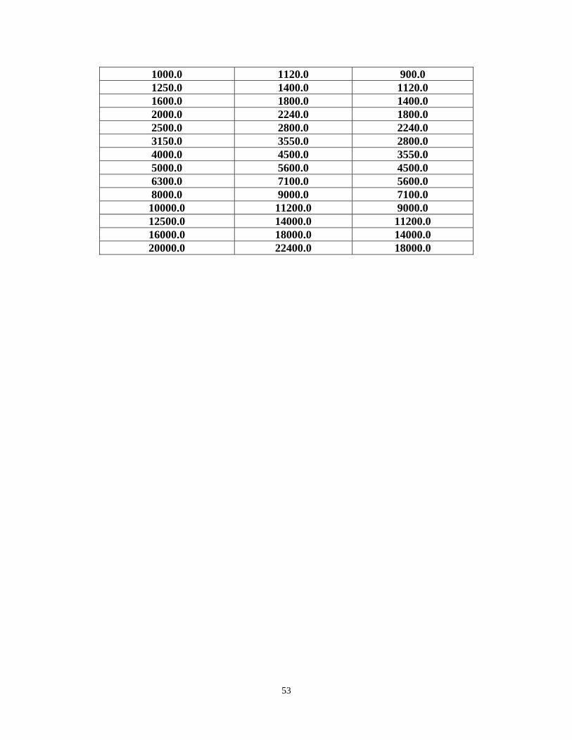
53

1000.0 1120.0 900.0 1250.0 1400.0 1120.0 1600.0 1800.0 1400.0 2000.0 2240.0 1800.0 2500.0 2800.0 2240.0 3150.0 3550.0 2800.0 4000.0 4500.0 3550.0 5000.0 5600.0 4500.0 6300.0 7100.0 5600.0 8000.0 9000.0 7100.0 10000.0 11200.0 9000.0 12500.0 14000.0 11200.0 16000.0 18000.0 14000.0 20000.0 22400.0 18000.0