Technical Report No. 3

BY 1. S. Lee

A ~ g ~ ~ t 1969

Reproduction in whole or in part is permitted by the U. I Government. Distribution of this document is unlimitez:l

TI0

https://ntrs.nasa.gov/search.jsp?R=19700016331 2018-06-29T20:14:35+00:00Z

NONLINEAR FILTERING TECHNIQUES WITH APPLICATIONS

TO THE STRAPDOWN ATTITUDE COMPUTATION 2

BY

J . S. Lee

Technical Report No. 3

Reproduction in whole or in par t is permitted by the U. S. Government. Distribution of this document is unlimited.

August 1969

P repa red under Grant NGR 22-007-068 Division of Engineering and Applied Physics

Harvard University - Cambridge, Massachusetts

for

NATIONAL AERONAUTICS AND SPACE ADMINISTRATION

i

NONLINEAR FILTERING TECHNIQUES WITH APPLICATIONS

TO THE STRAPDOWN ATTITUDE COMPUTATION

BY J. S. Lee

Division of Engineering and Applied Physics

Harvard University Cambridge Mas s achus etts

ABSTRACT

This reportt is devoted t o the solution of a special c lass of non-

l inear filtering problems and t o its applications to the attitude computa-

tional problem in a strapdown inertial navigation system.

A special c lass of nonlinear filtering problems is formulated in

chapter one to study the attitude computational algorithms in a strapdown

inertial navigation system,

particular mathematical model allows a direct iterative relation be obtained

between the successive estimates of the states. A ser ies of filters a r e

defined and algorithms a r e derived according to the computational load

allowed in a real t ime application.

It is shown that the characterist ics of this

Chapter two introduce the practical problem of the strapdown iner-

tial navigation system.

giving comparisons between the use of the derived algorithms and a commonly

used algorithm (the Taylor series second order algorithma”).

Monte Carlo simulation resul ts are presented

*

This report is a pa r t of a thesis submitted by the author July 1969 to Harvard University in par t ia l fulfilment of the requirements for the degree of Doctor of Philosophy.

This second order algorithm is a currently used attitude updating algorithm (see section 2, 4). It is obtained in a deterministic manner without taking the statist ics of the random environment into consideration. To avoid confusion with the second order nonlinear f i l ter to be derived in chapter one, we shall refer to this second order algorithm a s Algorithm A.

ii

Chapter three considers the attitude computation algorithms from a

m o r e restr ic ted and practical point of view, The approach is t6 impose a

complexity constraint which, in essence, res t r ic t s the filtering algorithm

to a particular f o r m with a set of parameters which a re , then, chosen

optimally to minimize an e r r o r cr i ter ion (the mean square e r ro r ) .

equations a r e given for the single axis rotation case.

for the single axis case show that substantial improvement in performance

can be obtained over the Taylor s e r i e s second order algorithm (refer to

the footnote of las t page), especially in the case where the statist ical

angular process is biased.

1

Explicit

The numerical resul ts

iii

TABLE OF CONTENTS

Page

ABSTRACT i

LIST O F SYMBOLS iv NOTATION vi

Chapter One A CLASS OF NONLINEAR FILTERING PROBLEMS

1.1 Introduction 1. 2 Formulation of the Problem 1. 3 Filter Structure 1. 4 Extention to a More General Model 1.5 Summary

Chapter Two APPLICATIONS O F NONLINEAR FILTERING ALGORITHMS TO STRAPDOWN ATTITUDE COMPUTATION

1 3 4 14 17

2.1 Introduction to the Strapdown Iner t ia l Navigation Sys tem 19 2, 2 Formulation 22 2, 3 The Optimal Filter for Single Axis Rotation Case 25 2 , 4 Numerical Results 28 2. 5 Discussion 41

Chapter Three FILTERS WITH COMPUTATIONAL CONSTRAINTS

3.1 Introduction 45 3. 2 Formulation of the Problem 46 3. 3 Single-axis Rotation with Statistically Uncorrelated

47 3. 4 Numerical Results 47 3. 5 Discussion 50

A ngula r Inc r erne nt s

REFERENCES 53

Appendix A DERIVATION OF AN UPDATING EQUATION 55 x.a. FOR P

1 1

Appendix B SOME CHARACTERISTICS O F DIRECTION

Appendix C EXPLANATION O F THE CONTRADICTIVE

Appendix D DERIVATION OF THE CONSTRAINED FILTER

COSINE MATRIX 59

RESULTS IN SIMULATION 3 O F CHAPTER T W O 63

FOR SINGLE-AXIS ROTATION CASE 67

ACKNOWLEDGEMENTS 75

iv

LIST OF SYMBOLS

Symbol

X i

i a

9

W i

i

i

- W

Q

Z i

H

E: i

i R

i Z A X. 1

A a. 1

pa i

‘i/iti

Ki/iti

Pi/iti

R ’ i

HI i

px a

Ki

i i

n-state vector to be estimated

rn-vector, random forcing function

m x m transition matrix

m-Gaussian vector (white noise)

E h i )

c ov(wi)

k-measurement vector

k x m matrix associated with the measurement z

k-vector , representing Gaussian and white noise

i

c ov( E: i)

s e t of measurements (zp, z L 2 - - - - - Y Zi)

conditionai mean of x. given Z

conditional mean of a. given Z

1 i

1 i A A T

E( ( ai - ai)(ai - ai) /Zi)

it1 . smoothed estimate of a . given Z 1

smoothed gain mat r ix

n Y n matrix

( 3HQ.H tR.) T 1 1

( =HI)

n x m matrix

(as defined by Eq. (1-32))

Page (defined)

4

8

9

9

9

9

10

11

c x V

Symbol Page (defined)

i A

X P

i

“1

“b

Y i

J

M

Q

( = 5 - Ki+lH@)

n x n matrix, E( (x - xi)(xi - xi) A A T /zi) i

3 x 3 direction cosine matrix

3 x 3 skew-symmetrical matrix

sca la r , body angular r a t e about j th axis

a vector in inertial coordinates

a vector in body coordinates

angular increment around jth axis in ith sampling interval

(defined by Eq. ( 2 - 9 ) )

(defined by Eq. (2-19))

sca la r , mean square e r r o r of estimating T i

weighting coefficient to be chosen optimally- sca la r

cumulative mean square error of (T (sca la r ) i

A - Ti)

scalar , E( Bi( 3) )

sca la r , cov(ei(3))

11

13

21

21

21

21

21

24

24

26

30

30

45

46

47

47

vi

NOTATION

Matrices will be denoted by upper case Roman letters. The vectors

will be denoted by lower case Roman or Greek letters.

considered to be the column vectors.

the superscr ipt T which stands €or transposition. Scalars will be explicitly

mentioned. The element

of a matrix A is denoted by a(i, j ) and the column vector associated with the

A l l vectors a r e

The row vectors a r e indicated by

For example; the performance index J is scalar .

matrix A is denoted by A(k) .

y / k ) .

Kronecker Delta, whereas, 6 ( t - T) will denote Dirac Delta,

The elemeni of a vector y will be denoted by

The s ta te x at t ime t. will be denoted by xi' 6.. will represent the 1 1J

The following symbols will be used to represent probability density

function and statistical evaluation of a random function;

p(x) = probability density function of x

p(x/ Z) = conditional probability density function of

x given the information Z

E( ) = expectation operator

Cov( = covariance operator

E(x /Z) = cdnditional mean of x given Z

CHAPTER ONE

A CLASS OF NONLINEAR FILTERING PROBLEMS

1.1 Introduction

R ecurs ive computation techniques for linear filters as derived by

Kalman [I] and others are well-known.

fully applied to many problems; for example, those related to orbit deter-

mination, attitude control and process control fields.

very little work has been done in applying some of the theoretical work

i n nonlinear filtering techniques that have been developed during the past

few years.

The techniques have been success-

In contrast to this

There a r e basically two approachs in attempting to solve problems

in nonlinear filtering. One approach is the use of a linearized model

about a n estimated state and the successive use of the linear filtering

techniques [2, Section 12.61.

conditional probability density function [3][4].

that for the continuous signal and measurement case, the conditional

probability density function satisfies a partial differential equation [5].

Similar equations have been derived for the case of continuous dynamics

with discrete measurements [6].

difficult to obtain. In general, approximations must be made. Examples

of the approximation techniques include the use of a Taylor series expansion

[6], moment generating sequences [7], and the use of approximate Gaussian

distribution functions [4].

of these algorithms to a reasonable problem of practical interest .

in terest to note that the results of a Monte Carlo simulations of eight different

nonlinear filtering algorithms [8] indicate that no one particular approxima-

tion scheme is uniformly better than any other.

The other approach requires the use of the

It has been shown by many

In all cases , analytic solutions are

There has been very little work on the application

It is of

-2 -

Most of the nonlinear recursive algorithms were intended for use

with very general nonlinear dynamic and measurement models, a s such,

the algorithms were extremely complex. Moreover, a lmost all der iva-

tions approached the problems in two steps: (1) the propagation and

prediction procedure based on all previous measurements , and (2) the

procedure of incorporating a n additional piece of data, the present

measurement. In general , approximation mus t be used in both steps.

This chapter considers a special class of nonlinear filtering problems

where the dynamics are of a special f o r m and where the measurements a r e

linear.

motivated f r o m the consideration of a pract ical problem involving the

attitude computation of a strapdown iner t ia l navigation system*'. [9].

This particular model has many pract ical applications and was

.I.

In view of the special character is t ics of the mathematical model,

it was found that a direct i terative relation between the successive

estimates of the state can be developed.

necessary to consider the two s t ep approximation as described in the

previous paragraph.

mation at every step.

In other words, it is no longer

The net resu l t is a m o r e efficient use of the infox-

The problem is formulated mathematically in Section 1. 2. The

derivation of the optimal f i l ter is given in Section 1. 3#.

m o r e general f i l tering problems is considered in Section 1.4.

Extention to

The details concerning the applications to the strapdown navigation sys t em a r e given in Chapter two.

- 3 -

1. 2 Formulation of the problem

The special c lass of nonlinear filtering problems to be considered

in this Chapter can be formulated as follows:

Given:

a) The nonlinear dynamics

x = f(CLi,Xi) i t 1

where

x. = n-vector representing the state

a. = m-vector forcing function 1

1

- E(xo) = x

0

COV(Xo) = Px 0

b) The dynamic equation governing the forcing function

a. = w1 t wi I t1

where

q = a known m x m transition matrix

w = m-Gaussian vector with i

'1 - - E((wi - wi)(wj - w.) ) = Q.6..

J 1 1J

c) Measurements

(1-3)

(1-4)

e =Ha. t E: i 1 i (1-5)

-4-

where

z = a k-vector representing physical data

K = k x m transformation matr ix i

6 = k-Gaussian vector with i

E(€.) 1 = 0

The Problem A

To find the best estimate of x A

denoted by xi, given measurements i’ z . ( j = I, 2, ~ L , , i) in the sense that x. is the conditional mean of x . given a l l

the data up to i.

the conditional mean has been proved 110, pp. 2171 to be the optimal

J 1 1

The reason €or taking the conditional mean of x. is that 1

estimator in the sense of minimizing the mean square e r ro r . Fig. 1.1

shows a block d iagram describing the above mathematical formulation.,

1. 3 Fil ter Structure

) represent the s e t of measurements ’ =it1 Let ZiS1 = (zl, zz9 z 3 , - - - - - - up to i-f-1.

that is

The problem is then tq evaluate the conditional mean of xiS1,

A x i f l = axi+l/zitll (1-7)

W e proceed by deriving an expression for the conditional probability density

function p(x i t 1 9 aitl/ZiSl). Using the fact that

p (a /b , c ) p(c/b) dc

- 5-

FIG. 1.1 BLOCK DIAGRAM OF THE FILTERING PROBLEM

- 6 -

where the integraiion is over the m-vector CL. and the n-vector x..

by applying Bayes formula, we have

Now, 1 1

where

Fur thermore , in (1-8)

Phi' ai/Zi+$ = Pki/ai9 Zi+$ P(ai/zitl) (1-10)

The first t e r m of the right hand s ide of (1-10) can further be decomposed as

= p(xi/ai, Zi) (1-ii) 1

since the density function p(ziS1/xi9 ai’ Zi) is the same as p(z itlPi’ Zi).

Combining (1-11) and (1-10) and substituting the remaining and (1-9) into

(1-8) give

-7 -

It follows that

and by definition, we have

(1-14)

To obtain an explicit expression for the nonlinear filter for a n

a rk i t r a ry f(a x.), approximations must be made. The approximation

technique is based on expanding f(a

where

i’ 1 A A

xi) in Taylor s e r i e s around a. and x i’ 1 i’

A a. = E(ai/Zi) (1-15) 1

A Direct observation of Eq. (1-3) and (1-5) shows that aitl satisfies the

solution of the well known Kalman filter. In other words

A - A (1-16) A T -1

0 2 = I p a. t Pa H R i (ziti - HI ai) tci ; a = a

0 i $1 is1 1

where P

known discrete matrix R iccati Equation.

is the standard m x m covariance matrix satisfying the well a i

A Consider now the problem of finding x F r o m (1-13) and (1-14), itl’

we have

(1-17)

Only in very rare cases can an exact solution of Eq. (1-17) be obtained. In

general, approximation must be used. One approximation scheme is the

Taylor s e r i e s expansion,

-8-

h A Expanding f(a x.) into Taylor s e r i e s around a. and x.':, yields i' 1 1 1

A A A {x - x.) t (higher order terms) (1-18) ai,xi i 1

A hierarchy of filters can be defined depending on the o rde r of the

expansion.

only the first te rm.

For example, the zeroth o rde r filter is defined by retaining

In which case, we find after substituting f(ai, xi) in A A

place of f(ai,xi) in (1-17) that

A A A x = f (a i 'Xi) i 4-1 (1-19)

Consider now the first order filter.

terms of (1-18)* The first t e r m is, obviously, f(a.,x.). The second t e r m is

It consists of using the first th ree A A 1 1

Let

(1-20)

(1-21)

4,

Eased on numerical resul ts in Section 2. 3 , the approximation of f(ai, xi) by its Taylor s e r i e s expansion as given by (1-18) proves to be agood one, at least in some problems.

-9 -

A is the smoothed est imate of a Then ailitl namely, the est imate based i'

It follows that 9 "it-1' on data z - - - - - 1'

a f A A (The 2nd term) = q & (ai/it1 - ai) i' 1

(1-22)

A The smoothed estimate ailitl is known [ll] to sat isfy the following equation.

(1-23) 'T '-1

Ki/itl - - pi/itl Hi R i

W i t h

- P ~i~ (HI pa. HI^ t ~ 1 1 - l ~ ~ pa i a. 1 1 1 i 1 1

pi/itl =

R ' = H Q . H T t R i i 1

I Hi = H

Substituting (1-23) into (1-22) yielc .s

(The 2nd t e r m ) = - Ki,itl (ziti - H (1-24)

It turns out that this additional correction term of (1-24) can be easi ly

incorporated to (1-19).

fore is applicable for r e a l time application,

2. 3 s e e m to indicate that significant improvement can be obtained by the

addition of this term.

KiIit1 can be precomputed and s tored and there-

Numerical resul ts of Section

Let us now consider the contribution of the third term in the expansion

of (1-18). Using (1-171, we s e e that

-10-

A 8

(The 3rd term) = - (xi - xi) p(xilai, Zi) p(dilZitl) dxi dai

(1-25)

T o evaluate the inner integral on the right hand side of (1-25), it is necessary

to make cer ta in assumptions concerning p(xi/ai, Zi).

appears to be that the random vectors x i’ 1 1

distributed with mean x 01. and conditional covariances P

A reasonable assumption

a. given Z . are jointly Gaussian A A >k

’Pa and PX., x: i i it 1

L L

Based on this assumption, it follows that

A -1 A (Xi .c x.) P(Xi/Qi9 Zi) dXi = PX& Pa (ai - ai)

1 1 1 i

where

A T = E((x - xi)(ai - ai) /Z i ) px a i i i

substituting (1-24) into (1-25) and using (1-23) shows that

- H l a i ) A (The 3rd term) =

(1-26)

(1-27)

(1-28)

Combining (1-28), (1-24) and (1-19)? it is seen that the first orde r filter can

be writ ten a s

A A A x = ffCLi,Xi) i $1

-1

i ’ i r i i 2 $i Px.a pa Ki/iti (ziti

* See Cosnrnents at the end of this section,

-11-

The only unknown in (1-29) is P

P

procedure as that leading to (1-29).

. i i

An iterative relation for updating x.a can be derived. The derivation follows essentially the same

X .a i i Although the derivation is tedious,

it is nevertheless straightforward (refer to Appendix A).

expression is

The final

(1-30) a f -1 T P 2 1. pi/i+l + k 2. Px.a pa pi/i+l) Ai Xitlaitl i’ i i ’ i i i i

where T Ai = @ - K H i 4-1

and

= (Q;’ + H ~ R ~ & H ) -1 H T R~ -1 Ki+l

(1-31)

(1-32)

C ornrne nts :

1. In evaluating Eq. (1-25), we assume that p(xi,ai/Zi) is Gaussian

distributed. This assumption is not s o dras t ic as it sounds.

close look of (1-26), we find that it is only the conditional mean of x. is of

interest .

Taking a

1

The conditional mean of xi is evaluated by

?$

We have approximated p(x a . /Z . ) by a Gaussian density function p (xi ,ai/Zi)

with mean and variance of p (x

p(xi, ai /Zi) .

density function, since p(ai/Zi) is Gaussian distributed,

i’ i 1 ag

a . / Z . ) equivalent t o the mean and variance of i’ 1 1 * This Gaussian approximation makes p (x./ai, Zi) a Gaussian

1

It is shown in Fig. 1. 2

-12-

PWOBABI LlTY DE NSlTY

FIG. 1.2 GAUSSIAN APPROXIMATION OF A DENSiTY FUNCTION

-13-

that p(xi/ai, Z.) may not be close to its Gaussian approximation, but a s

f a r as the value of the integral is concerned, the integration tends to 1

smooth out the i r regular i ty of p(x./a

conditional mean of x. close to the t rue conditional mean of x..

Z . ) and makes the approximated 1 i' 1

1 1

2, Recursive relations for the zeroth o rde r filter and the first

o rde r filter are given by Eqs. (1-19) and (1-29) respectively.

putation of Eq. (1-19) require the knowledge of a. which is given by (1-15)

and (1-16).

The com- A 1

A The computation of Eq. (1-29) requires a. as well as

1

which can be obtained f r o m (1-23) and (1-30). p i / i t l p P x.a. and Ki/itl

1 1

3 . Px which is the covariance of the e r r o r in the estimate is not i

needed in any of these recurs ive algorithms.

4. Higher o rde r f i l ters can be derived using the same approximation.

The second o rde r f i l ter

x.).

Eq. (1-33) shows the f o r m of a second o rde r filter.

is defined by using up to the second o rde r terms in the expansion of f(a

The derivation is straightforward but tedious hence it is omitted. i' i

x = ( ze ro o rde r term) t (first order term) it1

(1-33)

J

-14-

where

5, The first order filter as characterized by Eqs. (1-29) and (1-30)

turns out to be equivalent to the approach of using a linearized model along

an estimated s ta te and the successive use of the l inear filtering techniques

[2, Section 12. 61.

1. 4 Extention to a More General Model

The method which was used to der ive the recursive f i l ters in section 1. 3.

can also be used to obtain solutiofis related to a more general filtering

problem. Consider the following models:

a} The dynamics

x = f(Xi) f wi i ti

where x. and w. are the same as specified by (1-2) and 1-41, 1 1

b) The measurements

z =Hx . 4- E . i 1 1

(1-34)

(1-35)

where the statist ics of 8 . is given by (1-6). 1

The problem is to estimate the conditional mean of x, given measure- 1

ments up to i.

To obtain the best estimate of xi' we follow the techniques used in

section 1, 3 by deriving the conditional probability density and expanding

the nonlinear term into Taylor series.

Using the fact "chat

p(a/b) = s pCa/b,c) p(c/b) dc we have

-15-

and F

(1-36)

The integral xitl p(xit1/xi9 Z ) dxitl can be analytically car r ied out

) is Gaussian distributed, that is because of the fact that p(xitl/xi, Zit1

i 4-1 I

wkere

Substituting (1-37) into (1-36), yields

(1- 38)

T o obtain a n explicit expression of the nonlinear filter for a n

a rb i t ra ry f(xi), the nonlinear term f(x.) is expanded into Taylor s e r i e s

a r o u n d x o r

1 A i'

A (xi - x.) t (2nd order and higher order terms) A

1 ffx;) = f(Xi) -!-

(1-40)

A s before, a hierarchy of f i l ters can be defined:

1) The zero order filter

Substituting only the first term of (1-40) into (1-39), we have the

zero order fi l ter as

A (1-41) A x = f(xi) A t Ki (ziti - Hf(Xi))

i +1

-16-

A where Ki is given by (1-38).

the optimal es t imate of x

2) The first o rde r fi l ter

It is noted f r o m (1-41) that if f(xi) = f(xi)’ then A

is simply x i t1 i $1 given by (1-41).

The first o rde r fi l ter is obtained by substituting the first and the

second t e r m s of (1-40) into (1-39). The first t e r m is obviously given by

(1-41), and

A (The 2nd term) = (I - KiH) - axi ( x i [(xi - xi) p(xi7Zitl) hi (I -42)

The integral xi p(xi/Zitl) dxi is a smoothed est imate of xi’ Assuming

) andip(x. /Z.) a r e Gaussian, the second term can be approximated as P(Xi / Zi+l 1 1

A (The 2nd t e r m ) = (I - KiH) - - Hf(x . ) ) (1-43) 1. 1 Ki/itl (‘it1 1.

where

with

- P.H‘T (HI Pi Hi IT t HI Pi Pi/i+l = pi 1 1 1

R ’ = H Q i H T S R i i

and

A A T (Xi - Xi)(Xi - Xi) P(Xi/Zi) dxi Pi

Combining (1-43) and (1-41), we obtain the first order filter

(1-44)

-17

The recursive expression for updating P. is not available in analytic fo rm,

hence, for numerical realization, the approximated version is obtained by

expanding f(x.) into Taylor s e r i e s up to first order , and we have

1

1

T T -1 'it1 = Mi+l - MitlH (HMitlH + Ri) €3 Mitl

(1-45)

Comments:

1. (1-41) provides a simple zeroth order fi l ter which explicitly takes

the present measurement into consideration and which has the advantage

that Ki can be precalculated and stored. In fact, K. is constant i f Q. and R

a r e independent of i (see Eqs. (1-38) and (1-39)).

i 1 1

2. Higher order filters can be derived in the same way as the 1st

The first o rde r fi l ter given by (1-44) turns out to be equivalent to order.

the usual approach of using the linearized dynamic model applying the

recursive filtering techniques derived by Kalman [2, Section 12. 61.

3. The filtering algorithms derived in this section do not include

the filtering algorithms derived in previous section.

the general formulation of this section tends to neglect the special

character is t ics of the class of filtering problems discussed in last section,

The reason is that

1.5 Summary

A class of nonlinear filtering problems has been formulated in this

chapter intended to study the attitude computational algorithms in a s t rap-

down inertial navigation system. Recursive filtering algorithms which takes

advantage of the special character is t ics of this mathematical model have been

derived. Extention of the solution to more general dynamic and measurement

models has a lso been considered.

-19-

CHAPTER TWO

APPLICATIONS OF NONLINEAR FILTERING ALGORITHMS

TO

STRAPDOWN ATTITUDE COMPUTATION

2. 1 Introduction to the Strapdown Inertial Navigation System

The function of an inertial navigator is to indicate the attitude,

velocity and position of a vehicle with respect to a selected reference

frame using measurement obtained f rom onboard inertial instruments,

Broadly speaking, iner t ia l navigation systems can be divided into two

clas 5 es:

1.

2. The strapdown navigation system.

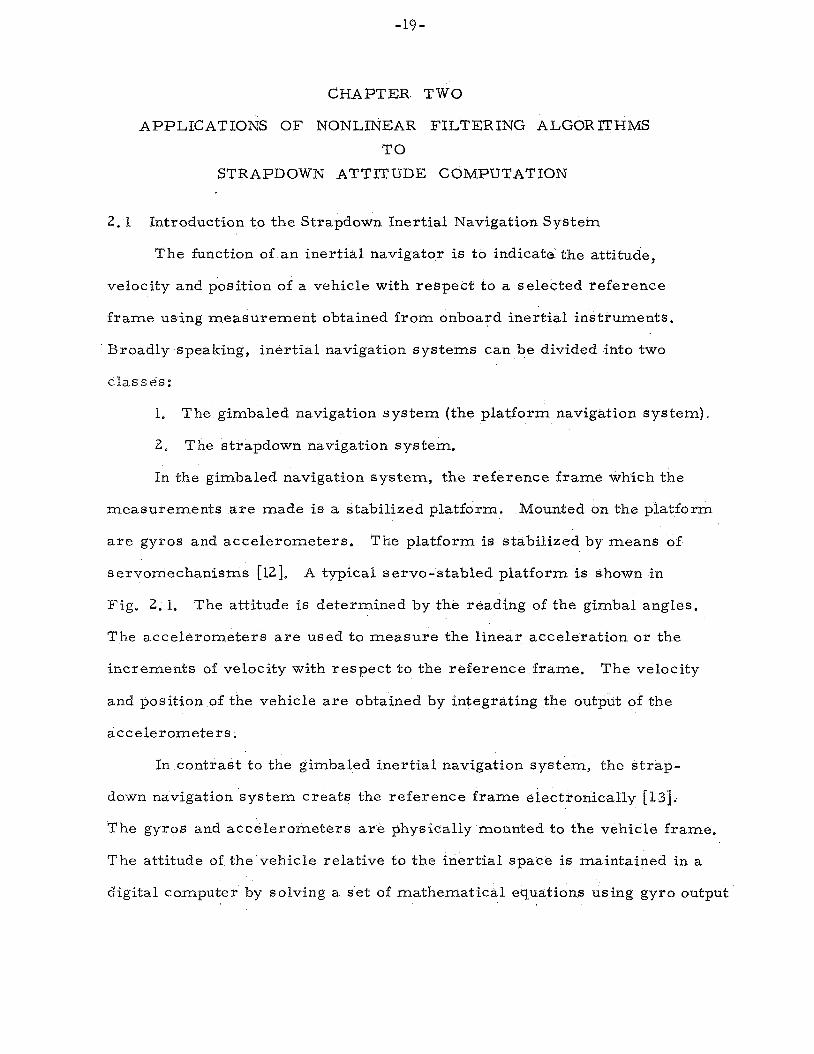
In the gimbaled navigation system, the reference frame which the

The gimbaled navigation sys tem (the platform navigation system).

measurements are made is a stabilized platform.

a r e gyros and accelerometers ,

servomechanisms [12].

Fig. 2 , l .

Mounted on the platform

The platform is stabilized by means of

A typical servo-stabled platform is shown in

The attitude is determined by the reading of the gimbal angles.

The accelerometers a r e used to measure the l inear acceleration o r the

increments of velocity with respect to the reference frame.

and position of the vehicle a r e obtained by integrating the output of the

accelerometers

The velocity

In contrast t o the gi-mbaled inertial navigation system, the s t rap-

down navigation sys tem creats the reference frame electronically [13].

The gyros and accelerometers itre physically mounted to the vehicle frame.

The attitude of the vehicle relative to the inertial space is maintained in a

digital computer by solving a se t of mathematical equations using gyro output

-20-

. r I

ROLL SERVO MOT(

i

STABILIZED PLATFORM

SERVO MOTOR

FIG. 2.1 GIMBALED INERTIAL iUAV1GATOR

-21-

as physical measurements.

the vehicle frame to the reference frame and many studies have been

Many parameters [9] can be used to re la te

conducted examining the use of these parameters and the various integra-

tion algorithms to update them [9][13][14],

hsed, for example, in the LEM Abort Guidance System, is the so called

direction cosine matrix. This is an orthonormal matrix of nine elements

giving the nine projections of a unit vector along the body coordinates to

the inertial coordinates (the reference frame).

A common set that has been a\

Let the 3x3 direction cosine matrix be represented by T(t). Then

it is well kQown that T(t) satisfies the matrix differential equation [13].

(2-1) d -T(t) = R ( t ) T( t ) at

where T ( t ) = I, an identity matrix, and R( t ) is a 3x3 matrix whose

elements represent the body angular rates' with respect to the vehicle

f rame ( o r body frame).

0

r o

i w ( z ) i n(t) = I - W ( 3 ) i

Let a. be the outputs of the accelerometers mounted on the body. b

Then, the acceleration with respect t o the inertial f rame is given by

4, -,- "LEM" stands for "Lunar Excursion Module".

-22-

T and aI provide the same information a s the gimballed angle and

The position and the the accelerometer output of the gimbaled system.

velocity of a vehicle can be conventionally obtained by double integration.

A block diagram comparing these two iner t ia l navigation system is shown

in Figure 2 .2 ,

An important problem associated with the strapdown navigation

sys t em is to find the computational algorithms for updating the trans-

formation ma t r ix T,

chapter.

This I s the problem that will be addressed in this

The advantages and disadvantages of the strapdown sys tem compared .I.

with a gimbaled sys t em are listed in the following*:

1. Advantages

i) Minimum mechanical complexity

ii) Small s ize , weight and power

iii) Packaging flexibility

iv) R eliability and maintainability

2. Disadvantages

i) Requires faSter onboarcl guidance computer

ii) High angular velocity exaggerats performance e r r o r s

2. 2 Formulation

A s described in section I. I, the class of filtering problems discussed

in Chapter One was motivated f r o m considering the pract ical problems

related to strapdown attitude updating.

the strapdown attitude updating problem is formulated into the c lass of

filtering problems of Chapter One.

In this section, we will show how

.Ir T

For detailed discussion please r e fe r to [I3],

- 2 3 -

information

GiMBALED SYSTEM

-24-

A s shown in (2-1), T(t) is updated by a s e t of differential equations

using the body angular ra tes W ( l ) , W ( 2 ) and W(3).

ments on the body angular ra tes are given in t e rms of incremental angle

f r o m which a(t) must be inferred (for instance, measurements from the

In practice, the measu re -

pulse-torque-rebalanced strapdown gyro [ 9 ] )

The measurements may be approximated by the equation

z = i t

where 6. is an additive noise term. 1

;g The solution of (2-1) at sampiing times can be approximated by

Y i = e i

(2-4)

(2-5)

<C

(2-5) i s the exact solution of (2-13, if Q(ti+l) commuts with yi [15] o r m o r e restrictively, if w ( j ) fo r j = 1,2 , 3, is constant over the sampling period

-25-

This discrete updating equation does not affect the orthonormal

condition of the transformation mat r ix T {see Appendix B).

expression for e

A n analytic

Y i is a lso given in Appendix €5.

F r o m power spec t ram analysis or by other statist ical methods

Qi(j), for j = 1,2,3, can be modelled as a Gaussian Markov random process.

Then, it is c lear f r o m ( Z - 3 ) , (2-4) and (2-5) that the problem of finding T i

is equivalent to the nonlinear fi l tering problem considered in chapter five.

T . corresponds to x. and 8. corresponds to ai* 1 1 1

For example, Eq. (2-5) can be written as a ninth order differential

equation

' ( 3 ) = eVi T , ( 3 ) it-1 1

where T( i ) , T(2) and T ( 3 ) a r e column vectors of the mat r ix T.

2, 3 The optimal Filter for Single Ax i s Rotation Case

Fop the case where the angular movement is around a single axis

only, an analytical expression exists for the optimal nonlinear filter.

can be used to establish a lower bound for the error variance.

derivation of optimal nonlinear fi l ter is given a s follows.

It

The

Assuming 0 , ( l ) = 0 and 0,(2) = 0 , for a l l i, Eqd- ( 2 - ecomes

A 0 . ( 3 ) Ti 1 T = e i -51 ( 2 - 4 )

- 2 6 -

where

Successive i terat ion o€ (2-6) gives

Define

'it1 = qi t k ( 3 ) ; V , = O

Eq. (2 -8 ) can be writ ten as

Ti+1 = e A%tl 0

where

The optimal nonlinear estimation of T in this case becomes it1

( 2 - 9 )

(2- lo}

( 2 -11)

- 2 7 -

A To evaluate Eq, (2-111, it is required to known vis1 and P

defined by

which are ‘it-1

Since & ( 3 ) has been assumed to be a Gauss-Markov processs f rom Eq. (2-9),

7 . will be a Gauss-Markov process [2, Chapter 113. By sequentially applying

the Kalman f i l ter , we can update q. and Py

1

P A

f o r all i, 1 i A‘i+l

Now to compute E[e /Z,,,], we make use of the character is t ic L l i

/ z , namely f A‘i+l function [a , pp. 1591 of then the elements of Efe

E[Cos ~ + ~ / z ~ ~ ~ ] and E[sin 7it-l/Zi+l], can be easily obtained.

character is t ic function of

The

is (refer to [IO, pp. 1591) given Z i t 1 i +1

(2-13)

where j =FR and CT is a dummy variable ( sca la r ) . Using Eq. (Z- l3) , we

have

-QPq A = e is1 Cos

and s imilar ly ,

( 2 -14)

{ 2 -15)

-28 -

Using Eqs. (2- io) , 42-14) and (2-l5), we have

A Sin nisi 7

i i i f

0

0

4

(2-16)

Eq. (2-11) and Eq. (2-16) give the optimal nonlinear estimate of Title

2,4 Numerical Results

For purpose of illustration, numerical work based on Monte Carlo

simulations were car r ied out using the recurs ive algorithms developed

in Chapter one.

procedures,

Figure 2. 3 is a block d iagram describing the simulation

For simplicity, it is assumed that the vehicle is subject to

a wide band noise' fluctuation (i. e.

the dynamic of the gyro output can be approximated as the output of the

purely random noise). In this case,

first order difference equation

where

and

eo( j ) = 0 with probability 1

for j = I, 2, 3

E(wi(j)) = 0

( 2 -17)

The measurements a r e given by equation (2-4) and the attitude matr ix

satisfies equations (2-5) where y , is given by (2 -3 ) . 1

- 2 9 -

-30-

F o r comparison purposes, we included in our numerical work a

typical strapdown attitude computation algorithm being used in cur ren t

LEM sys tem based on Taylor series expansions of e

by zi [16].

algorithm" has the form

Y i with 6 . replaced 1

This algorithm which is generaily called "the second order

where

c = i

To avoid confusion with the second order nonlinear fi l ter derived in

Chapter one, we shal l re fe r to (2-19) as ALGORITHM A.

The mean square e r r o r is adopted as the cr i ter ion for the evalua-

Let Ti be the t rue solution and let Ti be A

tion of the various algorithms.

the solution using a particular algorithm, Define

= T r a c e E((Ti - A Ti)(Ti - A T Ti) ) Ji (2-20)

then 5 . gives the mean square e r r o r at t ime t..

measu re of the expected magnitude square of the difference vector between

the vectors which are t ransfer red from the body coordinates to the iner t ia l

coordinates by using T . and T. respectively ( see Appendix B).

Physically, Ji is a 1 1

A

1 1

In the following, simulation resul ts are categorizkd into two classes:

c lass A , the single axis rotation case , and class B , the three axes rotation

case.

- 31-

C lass A : Single Axis R otation, Case

Four simulation resul ts will be presented. The first two simulations

are to show the advantage of applying the filters derived in Chapter one.

The third shows a contradictive resul t with explanations given in Appendix C .

The fourth simulation considers a pract ical problem associated with the

tes t of a strapdown gyro, It will be seen that in the case of higher noise

levels (e. i.

mance of the nonlinear filtering algorithms is much bet ter than that of

Algorithm A . The reason for this is given in Appendix C. The sample

means of square e r r o r in the first and second simulations are averaged

Q and R ) and lower correlation (e, i. , P(3) << 1.) the per for -

over 100 runs, whereas the third and fourth simulations are averaged over

50 runs and 15 runs respectively ( see Simulation 4 for the explanation of

15 runs).

Simulation 1 (Figure 2, 4)

This simulation demostrates the advantage of applying the second

o rde r nonlinear fi l ter .

The set of parameters is 2

2 Q = 0.1 radian

R = 0,1 radian

Bt3) = 8,3

E r r o r s are squared and averaged over 100 runs, A s shown in

Figure 2-4, the averaged square e r r o r s of applying the zero o rde r filter

and the first order f i l t e r a r e very close,,

improvement is obtained by the use of the second o rde r filter which is

It is seen that substantial

also Been to be very close to the t r u e optimal filter, The mean square

>;: R e f e r to Section 2 , 3 .

-32 -

5

1.0

.5

ZERO ORDER F i lTER

1 40

STEP i *

4

-33-

e r r o r generated by the use of Algorithm A is comparatively la rger which

is caused mainly by the truncation and the measurement errors,

Simulation 2 (Figure 2. 5)

It has been mentioned in Chapter one that the zeroth order filter

with a correction term as given by (2-24) will show significant improve-

ment over the zeroth order fi l ter i n many cases,

results of such a case,

tion t e r m provides a considerable improvement over the zeroth order

filter.

this additonal term (refer to section 1. 3) .

Figure 2.5 shows the

It is seen that the addition of this simple cor rec-

V e r y little additonal computations are needed for the inclusion of

In this simulation, we "cake 2

2

Q = 0. 0001 radians

R = 0.0001 radinas

P(3) = 0.5

In general, better resul ts can be expected f rom applying the zeroth

There are cases , however, o rder filter than €rom applying algorithm A.

where this is not true.

simulations we take

Such a case is shown in Figure 2. 6. In this

2

-17 2

Q = 0, 5856 x radians

R = 0. 5856 x 10 radians

P(3) = 1.

Detailed explanation of this contradictive simulation resul ts is given in

Appendix C .

-34-

n cn 2 3 c1z 0 0

CE w > 0

M 0 oe K w

c

U

0- '

t o-? 1

TERM

Q = 0.0001 R = 0.0001

( 3 ) = 0.5 Sampling Interval = TOO ms

fFlRST ORDER FILTER SECOND ORDER FtlTEf 'I

STEP i 32

F1G. 2.5 SiMULATION 2 (SINGLE AXIS ROTATION)

-35-

6

FIG. 2.6 SI 3 (SINGLE AXIS RorA-rlON)

- 3 6 -

Consider the problem associated with the tes t of a strapdown pulse-

rebalanced gyro [14].

the rate of rotation of the earth.

which is assumed to be subject t o random disturbances.

input r a t e W ( 3) can be modelled as an exponentially correlated random

process. The qiscrete fo rm is

The test is performed on a table which rotates a t

The gyro f r ame is fixed to the table

In this case , the

W i $1 (3) = P(3)Wi(3) +w;

with

B(3) = 0.9999

2 E[Uo(3)] = 10 degree /hr Cov[Wo(3)] = (0.05 degree /hr )

E[wr] = 0 2 E[wkwi] = (0.005 degree /hr ) Sik

where E[w (3) ] = 10 degree /hr corresponds to be ear th angular r a t e a t

the latitude of 45' and the uncertainty on the ear th ra te is expressed by

the covariance cov(W0(3)) = (0. 05 degree /hr ) .

0

2

A perfect gyro i s assumed and the only measurement e r r o r i s the

quantization e r r o r (1 sec) and the sampling interval is 0.1 second.

The purpose of this simulation is again to compare the resul ts of

using Algorithm A with the filtering algorithms derived in Chapter one.

For saving computing time, only 15 runs a r e simulated and averaged to

obtain the sample means and sample variances of e r r o r square. The

simulation results are presented in Fig. 2.7 and Table 2.1.

of square e r r o r which a r e computed over 15 runs may not be representative

of the t rue mean square e r r o r s .

The sample means

But this simulation resul t does indicate

- 3 7 -

15

ZERO ORDER F\LTER\ .

TIME ( S e d

ULA710N 4 (SINGLE AXIS ROTATION)

-38-

the tendency that the filtering algorithm is superior over Algorithm A ,

Two reasons are given below to support the above statement.

1. Simulation results showed that the square e r r o r s of applying

these fi l tering algorithms are smaller than that of applying Algorithm A

i n every run.

samples a r e used for both filtering algorithms and Algorithm A.

This is because that in the sirnulaticin process , the same

A bad

random sample (e. i.

its mean) will increase the sample mean square e r r o r s of applying the

filtering algorithms as well as that of applying Algorithm A .

words, bad random samples will generally hurt the performance of both

Algorithm A and the filtering algorithms.

the value of the random sample is far away f rom

In other

2. Fig. 2 . 7 shows that the sample means of square e r r o r generated by

using the filtering algorithms a r e much smal le r than that of using Algorithm A .

The sample variances of te rmina l square e r r o r a s given by Table 2 , l indicate

that in this simulation the sample t ra jector ies of square e r r o r obtained by

applying the fi l tering algorithms are close to its sample mean as compared

with those obtained by applying Algorithm A .

9

i Second 1 Optimal i Zeroth 1 First

1 Fi l t e r Order i Order j Order s [Algorithm A '

w. I I Filter i Filter Filter

Square i Error 1

t t f Sample 1 i I I

-9 : -20 0. 8 7 5 6 ~ 1 0 ~ ~ i 0, 1381 x 10 0.l3.50 x 1 0.1350 10. 1350 x10 Mean of t L 2

3 i I

I j

0.13OOx 0.8578 x 1 0 . 7 6 4 4 ~ low2' i 0 . 7 6 4 4 ~ J 0.7642 x 10 . f

i I ! 1

I > i -20 1

Sample i I 1 ' Variance of \ Square ! i

1 i i i Error i

Table 2.1 Numerical Results of Simulation 4.

-39-

Class B: Three Axes Rotation Case

In the following simulations, the attitude updating algorithms a r e

simulated under the circumstance that all three body axes of the vehicle

a r e under random disturbances.

in analytical form is available i-n this case.

One should note that no optimal filter

Simulation 5 (Figure 2. 8)

This simulation is concerned with a space vehicle in its orbit.

statist ical models for input rates W ( l ) , W ( 2 ) and W ( 3 ) a r e identical but

statist ically independent.

ra te models are given in the following

The

The statist ical values concerning the angular

E(wf) = 0

The sampling interval is taken a s lOOms and P = 0.9048 corresponding

t o 1 see in time constant of the continuous model.

out over a period of 30 s e c and the sampling interval is 0.1 sec.

c o m p t i n g time, the sample means and sample variances of square e r r o r

a re computed over EO runs.

been discussed in Sjmuiation 4.

The simulation is car r ied

For saving

The significance of this 10 run simulation has

Simulation result is presented in Fig, 2. 8

and Table 2, 2,

use of the zeroth order filter over the use of Algorithm A .

and second order filter do not show much improvement over the zeroth order

fiPter,

It is seen f rom Fig, 2, 8 that improvement is obtained by the

The first order

The sample variances a r e shown in Table 2,2, F o r comparison purpose,

-40-

lo-'

10-

r I // .-

I W

I / I

I I I I

I I

I

,----

ZERO ORDER FILTER 1st & 2nd ORDER FlLTER

30

S i ~ U ~ A ~ ~ ~ N 5 (THREE AX1 S ROTATION)

-41-

we also include in Table 2 . 2 the square root of sample variances and

sample means.

a r e smal le r a s compared with their sample means.

variance is the estimate of the t rue variance and since the sample mean

t ra jectory of Algorithm A is f a r apar t from those of filtering algorithms,

based on these, we a r e more confident to conclude that the filtering

algorithms a r e superior to Algorithm A.

It is seen that the square roots of sample variances

Since the sample

Simulation 6 (Figure 2, 9)

In simulation 3, we showed that in the case of very smal l but highly

correlated noise, Algorithm A may pe r fo rm better than the zeroth order

fi l ter in single axis rotation case.

have pretty much s imilar results.

the algorithm A is superior to the zeroth order f i l t e r and the application

of the first order fi l ter is desirable.

In this three axes rotation case , we

In Fig. 2, 9, it is clearly seen that

In this simulation, we take

2 R = Q = 0.5856 1 0 -' radian

2 .5 Discussion I

2. The simulation results presented in this chapter indicated that

simulation resul ts would be helpful in choosing an appropriate filtering

algorithm for a cer ta in random circumstance.

2 , The statist ical models which describe the angular motion and

the measurements a r e not necessary restr ic ted a s those specified by

(2-4) and (2-17).

designing a more sophisticated fi l ter ,

The gyro dynamics can be taken into consideration for

-42-

k 3 ” .ti

r”

1

I i 2

! i i I

i i

I I

-43-

3. Another advantage in applying the filtering algorithms of

Chapter one to the strapdown attitude computation is that the angular

rate which is needed for attitude control is obtained in the process of

computing TiS1 f rom the output of the Kalman filter (see Eq, (1-16)). A

I Square Root of Sample Variance

Table 2, 2 Numerical Results of Simulation 5

-45 -

CHAPTER THREE

FILTERS WITH COMPUTATIONAL CONSTRAINTS

3 , l Introduction

The filtering algorithms of Chapter one are derived mainly for

improving the accuracy of estimation; the computational complexity is

of secondary importance. The s t ructures of these filters are optimally

chosen by minimizing the cr i ter ion of mean square e r ro r . However,

many pract ical applications may require the filtering algorithm to be

of a f o r m that it can be computed efficiently, as such, many simplified

filters have been developed for the case of l inear dynamic and measilre-

ment models. Johnson [17] modified the Kalman filter into a fo rm which

has a s t ruc ture of smaller dimension than that of the signal process.

Athans, et al. [18][19] res t r ic ted the Kalman gain matrix to be piece-wise

constant or to be approximated by a simple function.

a scarc i ty of work dealing with the nonlinear filtering problems with

There seems to be

complexity constraints,

s t ructure of the fi l ter to a particular form with a s e t of parameters which

are, then, chosen optimally to minimize a n e r r o r cr i ter ion (the mean

square e r r o r ) ,

The approach used in this chapter is to f i x the

For illustration, the filters for the problem formulated in

section I. 2 is taken to be

where g is a fixed sample function which requires only a limited amount of

Computations and a.’s are coefficients which a r e to be optimally chosen to

minimize the mean square e r ro r .

to the strapdown attitude computation is considered in this chapter.

1

In particular9 the application of (3-1)

-46 -

3 . 2 Formulation of the Problem

C ons ider the strapdown attitude updating problem of Chapter two

where

; T = I y yi Ti 0

T,,, = e i 1 . l

and measurements

z = i ( 3 - 3 )

where 8. is a vector vandorn process.

filter is chosen as that of Algor i thmA (the second order algorithm, r e fe r

to Chapter two) but with the weighting coef€ficients to be chosen optimally,

The structure of the constrained 1

that is, the constrained filter is of the form

A A = (aifl) I t ai(2) Ci -t- ai(3f C i ) 2 Ti ; T o = I i+l

where Ci is defined by (2-15).

The set of a.(l),a,(Z) and a.(3> a re to be chosen to minimize the 1 1 1

cumulative mean square e r r o r

( 3 - 5 )

The approach which is used i n solving this problem is to t ransform

the stochastic optimization problem into deterministic problem by working

with mean and variance [I?]. In next section, the constraint f i l ter €or the

single axis rotation case is designed. Numerical results are presented in

-47 -

section 3 . 4 showing the advantage of this filtering algorithm.

to general case (three axes rotation case) is straightforward in principle

but very complicate in derivation. Hence the general th ree axes rotation

case will not be considered in this paper.

Extention

3. 3 Single-axis Rotation with Statistically Uncorrelated Angular Increments

Consider the single axis rotation case a s specified in section 2. 3,

Let us assume that e.(3) is taken to be a purely Gaussian random process

with mean M and variance Q, The problem is to find a.(j) of the constrained

f i l ter Eq. (3-4), for i = 0,1,2, . * . . a and j = 1 , 2 , 3 , such that the perform-

1

1

ance index J as given by Eq, (3-5) is a minimum with Ti and z. given by

Eq. (3-2) and Eq. (3-3) respectively. In general, analytic solution is not

available.

forward but tedious, hence it is given in Appendix D for interested readers .

In next section, the numerical results of applying the constrained fi l ter will

be given and comparison a r e made with Algorithm A .

1

The derivation for reaching a numerical solution is straight-

3 , 4 Numerical Results

TTpe optimization procedure in finding the optimal coefficients a.(l) , a ,( 2) 1 1

and a.(3) is ca r r i ed out by applying the well-known steepest descent gradient

method to the equivalent optimization problem a s derived i n Appendix D.

Here, we consider a case where

1

M = 0. radian

Q = 0.1 radian

R = 0, 001 radian

2

2

The iriitial guess ai(1)$ ai(2) and ai(3) for i = 1, N is chosen

to be those used in algorithm A , that is

-48 -

A f t e r optimization has been done, the set of optimal coefficients

ai(l), ai(2) and ai(3), for all i a r e tested in a Monte Carlo simulation.

Also included in this simulation are the filtering algorithms derived in

Chapter Qne, optimal fi l tering algorithm of Chapter two, and Algorithm A.

The results are plotted in Figure 3.1. It is seen that the constrained filter

gives a much lower J than the Algorithm A, although the computational load

is the same for both algorithms. Fur ther improvement can be obtained by

the use of the zerofh order filter but this is done at the expense of higher

computational load. It is noted thai the first order filter and the zeroth

order filter for this case are identical and is expressed by

A A A 9 i A A TiS1 = e Ti ; To = I

A where 8 is obtained through the use of Kalman-Bucy filter. i

It is interesting to point out that J obtained in the process of finding

the optimal ai( k) ‘ S is very close to the simulated J. Specifically,

2 = 0.665600 radian J~ imulat io ri

’optimal 2 = 0.654863 radian

This fact leads credence to the mathematical derivation developed in

Appendix D.

-49-

-50-

In the case that the mean of 8.(3) is non-zero (M f 0) , the use of the

constrainted filter is much more favorable than the use of Algorithm A as

shown in Figure 3 . 2 .

1

3 . 5 Discusqion

i) Section 3. 3 shows a case of designing the filtering algorithm under

computational constraints.

rotation around three axes case.

hence it will not be car r ied out here.

This development is ready to extend to the

However it is a very messy problem,

ii) The coefficient ai(l), ai(2) and ai(3), in general, will be time-

varying.

coefficients is desirable.

In the case of limited s torages, the design of piece-wise constant

The technique for designing piece-wise constant

control as given in [20] can be employed f o r this purpose.

-51-

4

A

I i

- 5 3 -

REFERENCES

[l] R . E . Kalman, "A new approach to l inear filtering and prediction problems, I ' TYans. ASME, BASIC ENGRG, Ser. D, Vol. 82, pp. 34-35, 1960.

[Z] A . E. Bryson and Y. C. €30, "Applied Optimal Control, Blaisdell, W altham, Mas s achus et ts 1969.

[3] Y. C. Ho and R . C , K. Lee, ItA bayesian approach to problems in stochastic estimation and control, IEEE Trans , Automatic Control, , pp. 333-339, October, 1964.

[4] H. Cox, "Recursive Nonlinear Fil tering, It Proceedings of the National Electronic Conference Vol. 21 pp. 7 7 0 - 7 7 5 , 1965.

[5] H. J. Kushner, "Nonlinear filtering: The exact dynamical equations satisfied by the conditional Mode, 'I IEEE Trans , Automatic Control, Vol. AC-12, No, 3 pp. 262-267, June, 1967.

[6] A H. Jazwinski, "Stochastic processes with application to filtering theory, 'I Report No. 66-6 Analytical Mechanics Associates Inc. November, 1966.

[7] H. 3. Kushner, "Approximations to Optima1 nonlinear filter, I '

IEEE Trans. Automatic Control pp. 544-556, October, 1967.

E, Schwartz and E. B. Stear , "A computational comparisovl of severa l nonlinear f i l ters , ' I IEEE Trans. Automatic Control pp. 83-86, February, 1968.

f8J

[9] R . T . Warner and J. 5 . Sullivan, "A study of the cri t ical c.omputationa1 problems associated with strapdown inertial navigation systems, I '

NASA Report, CR -968 United Aircraft Corporation April 1968.

[IO] A . Papoulis "Probability, Random Variable and Stochastic P rocess , I' Chapter 9 , Chapter ll, McCraw-Hill, 1965.

[11] Ranch, Tung, and Striebel, "Maximum likelihood estimates of linear dynamic sys tem," J. ALAA, Vole 3, No. 8, pp. 1445-1450, August 1965.

G. J. Thaler and R . C. Brown,"AnaTysis and design of feedback control systems, LVcGraw-Hill, Chapter 9, 1960.

[1Z]

[13] T . F. Wiener, "Theoretical Analysis of Gimballess inertial reference equiplnent using delta-modulated instruments, D. Sc. Thesis , M. I. T, , 1962.

-54-

[14] W . F. Ball, "Strapped-down Iner t ia l Guidance. The Coordinate Transformation Updating Problem, I ' Technical Report , U , S. Naval Ordnance T e s t station, China Lake, California, Apri l 1967.

E . Bellman, "Introduction to matrix analysis, I t Chapter 10, McGraw -Hill, 1960.

[I51

[16] D. 0. Benson and D E. Lev, "Evaluation of a second-order s t r ap - down system algorithm in a random environment, I t pp. 7-11, Report of Dynamics Research Corporation, October, 1967.

D . L. Kleinman, T. Fortman, and M. Athans, "On the design of l inear sys t ems with piecewise-constant feedback gains, ' I IEEE Trans. Automatic Control Vol. AC-13, No. 4, pp. 354-361, August 1968.

D. L. Kleinman and M. Athans, "The design of suboptimal l inear time-varying sys tems, ' I IEEE Trans . Automatic Control, Vol. AC-13, No. 2 , pp. 150-159, Apri l 1968.

[17)

[18]

[19] J . S. L e e and Y. C . Ho, "Analysis and Design of Integration Formulas for a Random Integrand, " Technical Report No. 2 , Harvard University, August 1968.

-55-

APPENDIX A

x,a. DERIVATION O F A N UPDATING EQUATION FOR P 1 1

I n this appendix, a n iterative expression for updating P wil l be X.cI i i

derived, where Pxaa is defined by (1-27). i i

By definition

U s i n g (l-l2],, we have

os after manipulations we have

%T i t1 is1

The last integral on the

(A - 2 )

r i g h t hand side of (A-2) can be Written as

where

-56-

Substituting

Defining A = 4 - K. . H @ (A -4) can be writ ten as i 1 I-1

(A -4)

(A-5)

A A Expanding f(a xi) along x a. in Taylor s e r i e s , we have i’ i’ I

A A . a f f(ai’Xi) = f (Ei ,Xi ) -I- -

t (Second order and higher order terms)

Substitutiqg (A-6) up to first o rde r into (A-5) and using the integration

resul ts in Chapter one, (A-5) is wri’cten into

P xi tlai t1

The last three t e rms on the right hand side of (A-7) are equal to

-57-

In the following, we a r e going t o show that

A A A - HQa.) aitl = 1 -I- M-iKi/i+l + Kitl)(zitl 1

This will make the last three terms of (A-7) equivalent to zero.

By definition,

we have

(A - 10)

The inner integral on the right hand side of (A-PO) is given by the t rans-

position of (A -31, hence (A-10) can be writ ten as

F r o m the definition of Ai, (A-11) is written into the fo rm

From Eq, (1-23), we have

(A -11)

(A -12)

(A -13

-58-

Substituting (A-13) into (A-7) , we have the i terative equation for

updating P x,a,’

P Xi+lai-tl

that i s ,

-59-

SOME CK

APPENDIX B

RACTERISTICS OF DIRECTION COSINE iM TRlX

Some characterist ics of the direction cosine matrix are considered

in the following,

Y i I. The analytical expression of e is given by

where yi is given by (2-3) and

0- i

Proof:

yi F r o m the definition of e

Since y . is a skew-symmetrical matrix, it can be shown that 1

where G i is given by (B-2).

Using (€3-4) and collecting even and odd terms in (B-3) , after

manipulation, (B -3) is converted into,

-60-

or

03-51 .I.

By summing up the se r i e s , we have

2 1 - COS 0 . ) y - t - (Sin oi) yi 1 I G i

Q. E. D.

It is interesting t a note that if 9,(j) for j = 1 ,2 , 3 is small , o r mathematically,

0 . 4 0, then the weighting coefficients of yi and y . in (B-1) approach 1 and $$,

respectively. In this case, (B-1) is of the fo rm

2 1 1

'i 2 e = I t y i t y i / 2

In essence, (B-6) is the Algorithm A which i s given by (2-15).

'i 2. e is a n orthonormal mat r ix

Proof:

Since y is a skew-symmetr ical matrix, we have i

Q. E. D.

3. If T . is a n orthonormal matr ix , then T is also a n orthonormal 1 i t1

V i matrix, where TiS1 = e

Proof:

Ti*

-61-

Since

. T TiTi = I

(E-8) is converted into

By (E-7), we have

T TitlTitl = I

Q.E. D

4,

Let R I and R b be a unit vector with respect to the inertial coordinates

Physical interpretation of the performance index given by (2-16).

and body coordinates respectively, then

where T is the t rue direction cosine matrix. A

b If the computed direction cosine matr ix T is used to t ransform R

into inertial coordinates, then we have

A T = T T X I

The difference vector between R - and R ' is

R; - R I = (T T

1 I ' T - P)RI

and the magnitude of the difference vector is

2; T A T A M = RI (T TT - I) (T TT - I) R I

-62-

Assuming R I being uniformly distributed over a unit sphere and A T being randomly distributed, then

T A 1 E(M2) = T r a c e TT - I) (T TT - I))] (33-10)

Using T TT = I, (B-10) is converted into

(33-11) i A A T A A T E ( d ) = T r a c e iE(I - T TT - T T 4 T T {

I or

A TI E(M ) = T r a c e iE((T - T)(T - T) 1 r A 2

L

= J

where J is the performance index given by (2-16).

W e conclude that the performance index J is a measure of the

expected magnitude square of the difference vector between the vectors

which a r e transformed from the body coordiaates t o the inertial coordi-

nates by using T and T r,espectively. A

-63-

APPENDIX C

EXPLANATION O F THE CONTRADICTIVE RESULTS IN

SIMULATION 3 O F CHAPTER TWO

Referring to Simulation 3 of chapter two and Figure 2 .6 , the

contradictive results of simulation 3 are explained by the following two

reasons:

1. For the numerical values used in simulation 3, the noise

level on both measurement and process a r e extremely

small that the magnitude of zi(3) is of the order of rad.

This small angular measurement makes Algorithm A a good

approximation of (2-51, since Algorithm A is the second

order Taylor s e r i e s expansion of ( 2 - 5 ) with 9.(3) replaced

by zi(3).

Algorithm A performs as well as (C-l), which is given by

1

In other words, i n the small angle situation,

:;: Az;(3j :;: >k Tiil = e Ti ; T = T

0 0

where A is specified by (2-7).

2. In the following, we present a mathematical analysis to

explain the result of simulation 3 . This analysis is based

on the previous argument and will show that in the case of

highly correlated ei(3) process (8(3) = 1. ), Algorithm A tends

to work bekter than the ze ro order filter.

Throughout the following derivation, I zi(3) I is assumed to be small

that we can replace Algorithm A by {C-l}- Terminal mean square e r r o r

-64-

produced by using Algorithm A as well as that produced by using the

zeroth order filter will be analytically derived to explain the contradic-

tive simulation results. .b

a) Derivation of JT generated by applying Algorithm A N

Iterativery using (C -11, we have

N-1

Similarly, fo rm 12-61, we have

N - l

i =O T N = e

The errar cr i ter ion given by (2-16) can be writ ten into

where E . is t'he measurement noise (white and Gaussian

with z e r o mean and R variance). Taking expectation of 1

(C-41, we end up with

(G -3 )

(C - 5 )

:;: It is noked that in ( C - 5 ) if R = 0, JN = 0.

-65 -

b) Derivation of JN generated by applying the zeroth o rde r filter

The zeroth order filter can be written as

(C - 4 )

A where 0 & ( 3) is the best estimate of 8 .( 3) obtained f r o m applying

Kalman-Bucy filter. Following the same derivation used in a). 1 1

We have

JN = Trace fz(1 F - e

where the sca l a r SN is given by (C-8)

Now, we are in a position to explain this contradictive simulation :;:

resul ts by comparing JN and JN as given by (C - 6 ) and (C -7) respectively.

In the case of highly correlated ei(3) process (B(3) = 1. ), the correlations

between (Bi(3) - Bi(3)) and ( 0 . ( 3 ) - 8.(3)), for i, j=1, ., . *.. * . . . * * . J J

would make Sn> (N-P)R, for la rger N, and hence

A A e $ N - L

However, in the ear ly steps ( N is smal l ) , the estimated e r r o r is 8:

smaller than the measurement e r r o r or J N < JN as is shown in Figure 2.6,

- 6 7 -

APPENDIX D

DERIVATION OF THE CONSTRAINED FILTER FOR

SINGLE -AXIS ROTATION CASE

Consider the stochastic optimization problem as formulated in

F o r clari ty, we restate the problem as follows. Section 3. 3.

1. The Attitude are updated by

Tifl = e y i T ; T = I i 0

Since the vehicle is rotating around one single body axis, only four

eiements i n T a r e affected by this rotation. A l l other elements remain

unchanged,

phys icaily updated by the following equation.

F r o m Eq. (D-L)> these four changing elements in T a re

or simply

= B T T i ~ l i i

!- \cos ~ ( 3 ) ,

L

r

where we have defined

; T = I 0

- 6 8 -

and

- 1 r̂

C O S 0 . ( 3 ) Sin 6;(3); 1

'i = ' i ;-Sin Bi(3) COS Bi(3)

I L I)

This notation is defined exclusively for use in this appendix.

2 . Measurement

I , 3,

4. Constrained filter

Bi(3) is a Gaussian white sequence with mean M and variance Q.

A 2 A A = (ai(l) I t ai(Z) C . 4- ai(3) C i )T i ; To = I Titi 1

where

5. Per formance index

N

J = E i =O 'i A

(Ti - Ti)fTi - Ti)

(D -4)

The problem is to choose the se t of weighting coefficients a . ( l ) , a.(2) 1 1

and a . f 3 ) such that J is a minimum. 1

For the convenience of later developement, Eq. (D-5) is rewri t ten

into

-69 -

where

A and Ti(k) is the kth column vector of Ti(k), s o is Ti(k).

Defining

P'k) i = E(T 1 .( k) Ti(k)T)

P(li) = E(Ti(k) ; for k = l , Z A A

i

A . Sfk) i = E(Ti(k) Ti(k)T)

we convert the stochastic optimization problem defined by Eqs. (D-2) ,

(0-31, (D-4) and (D-6) into a deterministic optimization problem as follows.

Using (D-8), (D-7) becomes

' N

where I?. (k'

de rived

and S'ki a r e computed by the iterative equations to be i ' i i

F o r the sake of convenience, @(3) will be simply denoted by Oi. In

'k) $!k' andS i ( k) , i ' 1 the following, the i terative equations fo r updating P

for k = 1, 2, will be derived.

Eqe (D -9) constitute a deterministic Optimization problem,

These iterative equations together with

-70-

1. From Eqs. (D-2) and (D-8), we have

T T = E(Ip.T.(k) T.(k) %. ) 1 1 1 1

The three distinct elements in P(k) 'are updated by i

(D -10)

2 Sin B i I i i 2Sin 8. COS 8 2 I ! c o s ei ! % 1 i '

I COS 0. Sin 8. ',

i 1 1 , = E! -Sin ei c o s 8 c o s 20

i ! '

where Eq. (D-11) is obtained directly from Eq. (D-10).

The initial condition of Eq. ID-11) is

t o

c

I

(D-11)

-71-

(0-11) is obtained by using the fact that ei is a purely random

sequence.

of (D-11) a r e obtained by using the character is t ic function [ lo , pp. 1601

The expected values of the elements on the right hand side

of the Gaussian random variable 20 They are i"

and

- 2Q ( c o s ZM) e 2 x(cos e : ) = - t 1 2 2

2 2 - 2Q (Cos 2M) e 2 E(Sin 9,) = - -

E(Sin g i Cos 0 . ) = 1 (Sin 2M) e - 2Q 1

2, F r o m (D-Z), (D-4) and (D-8) , and defining

2 i Di = ai(l) I f ai(2) C. 1 1 f a.(3) C

we have

. The three 'distinct elements a r e updated by

(D-13)

(D-14)

- 7 2 -

with initial conditions

rp i . ,e expected values of the e-xnents on the right hand side of Eq. D -1

2 2 2 - 2ai(l)ai[3)(R f Q t M ) E(Di(l, 1) ) = ai(l)

t a . (3)2(3(R 1. t Q)2 -t 6M2(R t Q)+ M4)

3. From Eqs. fD-4) and (D-8) . we have

(D-15)

I are

T = E(D.S.P . 1 1 1

-73 -

The four distinct elements a r e updated by

I i i !-D.f192) Cos 8 Di(l , l) Cos B i

1 i = E{ 1

h

D. (1,l) Sin O i

-D.(l,Z) Sin Bi

D.(19 1) Cos 8

D.(19 2) Sin e d

D.(191) Sin 8 .

1 1

i 1 1 ' 1

f D.(l, 2) Cos B i

D.( l , 1) C O S B i

1 i 1

i i

-Di(l, 2) Cos B i i

1

-/

with initial condition

9

(D-16)

(D-17,)

-74-

By using the character is t ic function [ lo , pp. 1601 of B i and its derivatives

the expected values of the elements of Eq. (D-16) are

-8Q E(D.( l , l ) 1 C O S e.) 1 = (a.(l) .1 - ai(3)R) Cos M e .

t a.(3)[(Q2 - Q - M 2 ) + 2MQ S'in M]e -$Q 1

E(D.(1,2) C O S 9.) = ai(2)[M Cos M - Q Sin Mle -8Q 1 7.

E(D.(l, 1) Sin ei) = (ai(l) - ai(3)R) Sin M e -&Q 1

2 -9Q t ai(3)f(Q2 - Q - M ) Sin M - 2MQ Cos M]e

and

E(D.(1,2) Sin 0 . ) = a.(2)[Q Cos M t M Sin M]e -$Q 1 1 1

The equivalent optimization problem:

Now the problem is to choose ai(I)?a . (Z) and ai(3) for i = 1, - - - - - - - - 7N 1

such that J given by (D-6) is optimized subject to (D-ll), (D-14) and (D-16) as

constraints.

which resul ts in a two point boundary value problem.

in analytical form. is available.

applying the numerical optimization techniques ~

Variational calculus can be applied t o the. solution of this problem

However, no solution

Numerical solution can be obtained through

-75-

ACKNOWLEDGEMENTS

I wish to thank Dr . F. Tung, NASA, and Professor Y. C . €30,

Harvard University, f o r their continuous guidance and encouragement

throughout the r e sea rch work.

the results of many stimulating discussions with Dr. Tung and Professor Ho.

Much of the mater ia l presented here is