TECHNICAL

R E P O R T

Institut fur Informationssysteme

Abteilung Datenbanken und

Artificial Intelligence

Technische Universitat Wien

Favoritenstr. 9

A-1040 Vienna, Austria

Tel: +43-1-58801-18403

Fax: +43-1-58801-18493

sek@dbai.tuwien.ac.at

www.dbai.tuwien.ac.at

INSTITUT FUR INFORMATIONSSYSTEME

ABTEILUNG DATENBANKEN UND ARTIFICIAL INTELLIGENCE

The D-FLAT System: User Manual

DBAI-TR-2017-107

DBAI TECHNICAL REPORT

2017

DBAI TECHNICAL REPORT

DBAI TECHNICAL REPORT DBAI-TR-2017-107, 2017

The D-FLAT System: User Manual

Bernhard Bliem 1 Marius Moldovan 1 Stefan Woltran 1

Abstract. D-FLAT is a software system that combines Answer Set Programming (ASP)with problem solving on tree decompositions and can serve as a rapid prototyping tool fordesigning dynamic programming algorithms over tree decompositions in a fully declarativeway. In terms of expressibility, it was shown that using D-FLAT can solve any problemexpressible in monadic second-order logic in linear time given that the problem instancehas bounded treewidth. In this report, we summarize all features of D-FLAT and highlightfunctionality that has been added recently. We give a comprehensive overview of our systemand provide several examples.

1TU Wien. E-mail: {bliem,moldovan,woltran}@dbai.tuwien.ac.at

Acknowledgements: This work has been supported by the Austrian Science Fund (FWF) undergrants P25607 and Y698, and by the Vienna University of Technology special fund “InnovativeProjekte” (9006.09/008).

Copyright c© 2017 by the authors

Contents1 Introduction 4

2 Background 72.1 Answer Set Programming . . . . . . . . . . . . . . . . . . . . . . . . . . . . . . . 7

2.1.1 Syntax . . . . . . . . . . . . . . . . . . . . . . . . . . . . . . . . . . . . 72.1.2 Semantics . . . . . . . . . . . . . . . . . . . . . . . . . . . . . . . . . . . 82.1.3 Complexity and Expressive Power . . . . . . . . . . . . . . . . . . . . . . 92.1.4 ASP in Practice . . . . . . . . . . . . . . . . . . . . . . . . . . . . . . . . 10

2.2 Tree Decompositions . . . . . . . . . . . . . . . . . . . . . . . . . . . . . . . . . 112.2.1 Concepts and Complexity . . . . . . . . . . . . . . . . . . . . . . . . . . 112.2.2 Dynamic Programming on Tree Decompositions . . . . . . . . . . . . . . 13

3 The D-FLAT System 173.1 System Overview . . . . . . . . . . . . . . . . . . . . . . . . . . . . . . . . . . . 173.2 Constructing a Tree Decomposition . . . . . . . . . . . . . . . . . . . . . . . . . 183.3 Item Trees . . . . . . . . . . . . . . . . . . . . . . . . . . . . . . . . . . . . . . . 20

3.3.1 Extension Pointers . . . . . . . . . . . . . . . . . . . . . . . . . . . . . . 203.3.2 Item Tree Node Types . . . . . . . . . . . . . . . . . . . . . . . . . . . . 223.3.3 Solution Costs for Optimization Problems . . . . . . . . . . . . . . . . . . 23

3.4 D-FLAT’s Interface for ASP . . . . . . . . . . . . . . . . . . . . . . . . . . . . . 233.4.1 General ASP Interface . . . . . . . . . . . . . . . . . . . . . . . . . . . . 243.4.2 Simplified Interface for Problems in NP . . . . . . . . . . . . . . . . . . . 29

3.5 D-FLAT’s Handling of Item Trees . . . . . . . . . . . . . . . . . . . . . . . . . . 323.5.1 Constructing an Uncompressed Item Tree from the Answer Sets . . . . . . 333.5.2 Propagation of Acceptance Statuses and Pruning of Item Trees . . . . . . . 333.5.3 Propagation of Optimization Values in Item Trees . . . . . . . . . . . . . . 343.5.4 Compressing the Item Tree . . . . . . . . . . . . . . . . . . . . . . . . . . 34

3.6 Materializing Complete Solutions . . . . . . . . . . . . . . . . . . . . . . . . . . 353.7 Further Functionality . . . . . . . . . . . . . . . . . . . . . . . . . . . . . . . . . 36

3.7.1 Default Join . . . . . . . . . . . . . . . . . . . . . . . . . . . . . . . . . . 363.7.2 Built-in Counters . . . . . . . . . . . . . . . . . . . . . . . . . . . . . . . 373.7.3 Lazy Evaluation . . . . . . . . . . . . . . . . . . . . . . . . . . . . . . . 38

3.8 Command-Line Usage . . . . . . . . . . . . . . . . . . . . . . . . . . . . . . . . 40

4 D-FLAT in Practice 454.1 Problems in NP . . . . . . . . . . . . . . . . . . . . . . . . . . . . . . . . . . . . 45

4.1.1 Minimum Dominating Set . . . . . . . . . . . . . . . . . . . . . . . . . . 454.1.2 Connected Dominating Set . . . . . . . . . . . . . . . . . . . . . . . . . . 47

4.2 A Problem beyond NP: Subset-Minimal Dominating Set . . . . . . . . . . . . . . 494.3 Default Join in Practice . . . . . . . . . . . . . . . . . . . . . . . . . . . . . . . . 504.4 Built-in Counters in Practice . . . . . . . . . . . . . . . . . . . . . . . . . . . . . 51

2

4.5 Lazy Evaluation in Practice . . . . . . . . . . . . . . . . . . . . . . . . . . . . . . 55

5 Conclusion 57

3

1 IntroductionComplex reasoning problems over large amounts of data arise in many of today’s application do-mains for computer science. Bio-informatics, where structures such as proteins or genomes have tobe analyzed, is one such domain; querying ontologies like SNOMED-CT is important in medicine,another such domain. Applications like the ones mentioned provide a great challenge to push thebroad selection of logical methods from Artificial Intelligence and Knowledge Representation to-ward practical use. To successfully face this challenge, the following considerations appear crucial.

First, for formalizing and implementing complex problems, declarative approaches are de-sired. Not only do they lead to readable and maintainable code (compared to C code, for instance),they also ease the discussion with experts from the target domain when it comes to specifyingtheir particular problems. Database query languages, which serve this purpose well in the businessdomain, are often too weak to capture concepts required in other domains, for instance, reacha-bility in structures. A particular candidate for such an advanced declarative approach is AnswerSet Programming (ASP) [23, 39] for which there are sophisticated solvers available that offer highefficiency and rich languages for modeling the problems at hand. A particular feature of ASP isthe so-called Guess & Check methodology, where a guess is performed to open up the search spacenon-deterministically and a subsequent check phase eliminates all guessed candidates that turn outnot to be solutions. Since many complex problems have a combinatorial structure, this methodallows for a succinct description of the problem to be solved.

Second, handling computationally complex queries over huge data is an insurmountable obsta-cle for standard algorithms. One potential solution is to exploit structure. This is motivated by thefacts that, for example, molecules are not random graphs and medical ontologies are not arbitrarysets of relations.

A prominent approach to exploit structure is to employ tree decompositions (see, e.g., [21]for an overview). This is particularly attractive because it allows us to successfully decomposeany problem for which a graph representation can be found. Even more important, via Courcelle’sfamous result [27] it is known that many problems can be efficiently solved with dynamic program-ming (DP) algorithms on tree decompositions if the structural parameter “treewidth” is bounded,which means that the graph resembles a tree to a certain extent. The main feature of such an ap-proach is that what causes an explosion of a traditional algorithm’s running time can be confined toonly this structural parameter instead of mere input size. Consequently, if the treewidth is bounded,even huge instances of many problems can be solved without falling prey to the exponential explo-sion. Empirical studies [6, 43, 44, 45, 51, 56, 57] indicate that in many practical applications thetreewidth is usually indeed small. However, the implementation of suitable efficient algorithms isoften done from scratch, if done at all.

All this calls for a suitable combination of declarative approaches on the one hand and structuralmethods on the other hand.

We focus here on a combination of ASP and problem solving via DP on tree decompositions.For this, we have implemented a free software system called D-FLAT1 for rapid prototyping ofDP algorithms in the declarative language of ASP. The success of ASP for solving hard problems

1http://www.dbai.tuwien.ac.at/research/project/dflat/system/

4

witnesses that this language is well suited for a lot of problems, and in fact it turns out that ASP isoften also well suited for parts of such problems. This makes it an appealing candidate for workingon decomposed problem instances.

The key features of D-FLAT are that

• ASP is used to specify the DP algorithm by declarative means (since ASP originated in partfrom research on databases, it can be conveniently used to specify table transitions which arethe typical operations in DP);

• the burden of computation and optimization is delegated to existing tools for finding treedecompositions and to ASP solvers;

• D-FLAT relieves the user from tedious non-problem-specific tasks, but stays flexible enoughto offer enough power to solve a great number of problems;

• in particular, D-FLAT can be applied to any problem whose fixed-parameter tractabilityfollows from Courcelle’s Theorem [27] in the sense that, given a suitable specification of theDP algorithm of the considered problem together with a tree decomposition of the instance,D-FLAT is able the solve the problem in fixed-parameter linear time (see [17]).

Comparing the standard way of Answer Set Programming with the dynamic programming ap-proach via D-FLAT, the following differences and implications have to be emphasized:

• In standard ASP, an encoding describes how to solve the problem at hand when the instanceis given in its entirety; we call such encodings also monolithic. An ASP solver is onlyinvoked once and delivers the solutions.

• In D-FLAT, the problem instance is first decomposed and the encoding has to follow acertain dynamic programming style. In fact, the encoding is called many times on differentcomponents of the instance and the ASP solver delivers solutions to subproblems, which arethen, roughly speaking, put together accordingly by D-FLAT.

• Finding such a dynamic programming encoding that works on tree decompositions mightbe considerably more involved than finding a monolithic encoding. However, the D-FLATapproach might help to overcome the well-known grounding bottleneck of ASP (since theencoding is only applied to small fractions of the instance) and allows for a straightforwardparallelization since certain components can be solved in parallel (see [14]). Finally, for in-stances of small treewidth, D-FLAT can potentially outperform the standard ASP approach.

D-FLAT is free software written in C++ and internally uses the answer set solving systemsGringo and Clasp [38], as well as the htd framework [3, 4] for heuristically generating a treedecomposition of the input.

Since D-FLAT version 1.0.0, which has been described in a previous report [1], we have im-proved the system in terms of efficiency and additional features. On the one hand, D-FLAT nowuses the decomposition framework htd. On the other hand, we added new functionality to D-FLAT

5

such as a lazy evaluation mode which is especially useful for search problems and for optimizationproblems, where it allows for anytime optimization [14]. Moreover, we added built-in counters,which take over even more of the computational burden from ASP [2]. We used the tool for im-plementing decomposition-based algorithms for various problems from diverse application areas,which demonstrates the usability of the method.

This report is structured as follows: We first provide background on Answer Set Programmingand tree decompositions in Section 2. In Section 3, we then present the current version 1.2.5 ofD-FLAT and describe its components, as well as the newer functionality, in detail. Subsequently,we turn to practical applications in Section 4, where we present D-FLAT encodings for severalproblems and illustrate how to use D-FLAT in practice. We conclude this work with a summary inSection 5, where we also mention some related work.

This report extends and reuses several parts from the first progress report from 2014 [1]. Themain changes appear in Sections 3.2 and 3.7, where we discuss the decomposition library andthe new functionality. Accordingly, we adapted Tables 2–5, which list the internal predicatesfor D-FLAT encodings, as well as Section 3.8, which describes the command-line interface ofD-FLAT. We substantially reorganized Section 4, where we illustrate the usage of D-FLAT onsome examples. That section now puts a focus on examples that make use of the new functionalities(Sections 4.4 and 4.5).

6

2 BackgroundIn this section we describe the underlying concepts of the D-FLAT system. We largely follow thepresentation in [12]. Section 2.1 is devoted to Answer Set Programming and Section 2.2 coverstree decompositions.

2.1 Answer Set ProgrammingSince NP-complete problems are believed not to be solvable in polynomial time, in principle weprobably cannot do better than an algorithm that guesses (potentially exponentially many) candi-dates and then checks (each in polynomial time) if these are indeed valid solutions. Logic program-ming under the answer set semantics is a formalism that allows us to succinctly specify programsthat follow such a Guess & Check approach [10, 39, 46]. Answer Set Programming (ASP) denotesa fact-driven programming paradigm in which one writes a logic program to solve a problem suchthat the answer sets of this program correspond to the solutions of the problem. Easily accessibleintroductions are given in [23, 47]. In [53, 50], ASP is proposed as a paradigm for declarativeproblem solving. A crucial observation is that the answer set semantics allows a logic program tohave multiple models, which allows for modeling non-deterministic computations in a natural way.Since answer sets derive from nonmonotonic reasoning, also the concept of negation as failure isimplied. [26]

2.1.1 Syntax

In the following, we suppose a language with predicate symbols having a corresponding arity(possibly 0), as well function symbols with a respective arity, and variables. Function symbolswith arity 0 are called constants. By convention, variables begin with upper-case letters whilepredicate and function symbols begin with lower-case letters.

Definition 1. Each variable and each constant is a term. Also, if f is a function symbol witharity n, and t1, . . . , tn are terms, then f(t1, . . . , tn) is a term. A term is ground if it contains novariables. If p is an m-ary predicate symbol and t1, . . . , tm are terms, then we call p(t1, . . . , tm)an atom. A literal is either just an atom or an atom with the symbol “not” put in front of it. Anatom or literal is called ground if only ground terms occur in it.

Using these building blocks, we define the following central syntactical concept.

Definition 2. A logic program (sometimes just called “program” for short) is a set of rules of theform

a← b1, . . . , bm, not bm+1, . . . , not bn

where a and b1, . . . , bn are atoms. Let r be a rule of a program Π. We call h(r) = a the headof r, and b(r) = {b1, . . . , bn} its body which is further divided into a positive body, b+(r) ={b1, . . . , bm}, and a negative body, b−(r) = {bm+1, . . . , bn}.

7

We call a rule r safe if each variable occurring in r is also contained in b+(r). In the following,we only allow programs where all rules are safe.

If the body of a rule r is empty, r is called a fact, and the← symbol can be omitted. A rule (ora program) is called ground if it contains only ground atoms. Note that we sometimes write

← b1, . . . , bm, not bm+1, . . . , not bn.

A rule of this form (i.e., without a head) is called an integrity constraint and is shorthand for

a← not a, b1, . . . , bm, not bm+1, . . . , not bn

where a is some new atom that exists nowhere else in the program.

The intuition behind a ground rule is the following: If we consider an answer set containingeach atom from the positive body but no atom from the negative body, then the head atom must bein this answer set. An integrity constraint, i.e., a rule with an empty head, therefore expresses thata set containing each atom from the positive body but none from the negative body cannot be ananswer set. Of course, we still need to define the notion of answer sets in a formal way, which wewill now turn to.

2.1.2 Semantics

Since the semantics of ASP, as we will see, deals only with variable-free programs, we first requirethe notion of grounding a program, i.e., instantiating variables with ground terms, for which thefollowing definitions are essential.

Definition 3. Given a logic program Π, the Herbrand universe of Π, denoted by UΠ, is the set of allground terms occurring in Π, or, if no ground terms occur, the set containing an arbitrary constantas a dummy element. The Herbrand base of Π, denoted by BΠ, is the set of all ground atomsobtainable by using the elements of UΠ with the predicate symbols occurring in Π. The groundingof a rule r ∈ Π, denoted by grΠ(r), is the set of rules that can be obtained by substituting allelements of UΠ for the variables in r. The grounding of a program Π is the ground programdefined as

gr(Π) =⋃r∈Π

grΠ(r).

We now define the answer set semantics that have first been proposed in [40]. To this end, wefirst introduce the notion of answer sets for ground programs.

Definition 4. Let Π be a ground logic program and I be a set of ground atoms (called an interpre-tation). A rule r ∈ Π is satisfied by I if h(r) ∈ I or b−(r) ∩ I 6= ∅ or b+(r) \ I 6= ∅. I is a modelof Π if it satisfies each rule in Π. We call I an answer set of Π if it is a subset-minimal model ofthe Gelfond-Lifschitz reduct of Π w.r.t. I , which is the program defined as

ΠI ={h(r)← b+(r) | r ∈ Π, b−(r) ∩ I = ∅

}.

8

Having introduced the notion of answer sets for ground programs, we can now state the answerset semantics for potentially non-ground programs by means of their groundings.

Definition 5. Let Π be a logic program and I ⊆ BΠ. I is an answer set of Π if I is an answer setof gr(Π).

Therefore, answer sets of a program with variables can be computed by first grounding itand then solving the resulting ground program. This is mirrored in ASP systems which typicallydistinguish a grounding step from a subsequent solving step and can thus be divided into a grounderand a solver component. D-FLAT uses the grounder Gringo and the solver Clasp [38].

2.1.3 Complexity and Expressive Power

Naturally, questions of computational complexity and expressive power of ASP arise. A survey ofresults is given in [28]. We will now mention results that are especially important for our purposes.

The unrestricted use of function symbols leads to undecidability in general [24, 7]. In thiswork, we therefore do not allow function symbols of positive arity to be nested, which is a veryrestrictive condition but already gives us a convenient modeling language. In this case, decidingwhether a ground logic program has an answer set is NP-complete [49].

We are of course not only interested in the propositional case but also in the complexity in thepresence of variables. The use of variables allows us to separate the actual program from the inputdata, so ASP can be seen as a query language where the (usually non-ground) program can beconsidered a query over a set of facts as input.

This dichotomy between the actual program and the data serving as input should be takeninto account when studying the complexity of non-ground ASP. As mostly we are dealing withsituations where the program stays the same for variable data (cf. Section 2.1.4 for an exampleencoding for the GRAPH COLORING problem), it is reasonable to consider the data complexity ofASP. By this we mean the complexity when the program (consisting of a set of rules with possiblynon-empty bodies) is fixed whereas only the set of facts representing the data changes.

Let Π be a logic program and ∆ be a set of facts. Deciding answer set existence of Π ∪ ∆ isNP-complete w.r.t. the size of ∆ (i.e., when Π is fixed). This is because when Π is fixed and only∆ varies, the size of gr(Π ∪∆) is polynomial in the size of ∆.

The aforementioned complexity results give us insight into how difficult it is to solve ASPprograms. A related question is which problems can actually be expressed in ASP. Informally,when we say that ASP captures a complexity class, it means that for any problem in that classwe can write a uniform logic program (i.e., a single logic program that stays the same for allinstances) such that this program together with a set of facts describing an instance has an answerset if and only if the instance is positive. It has been shown that ASP captures NP [55], and alsoevery search problem in NP can be expressed by a uniform ASP program [48]. There are variousgeneralizations of the presented ASP syntax and semantics in the literature. For instance, allowingthe use of disjunctions in rule heads (as in [41]) yields higher expressiveness at the cost of ΣP

2 -completeness for the problem of deciding answer set existence for ground programs [32, 33].

9

a b c

d e f

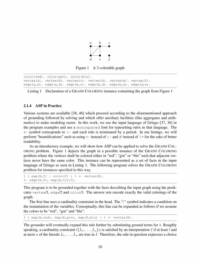
Figure 1 A 3-colorable graph

color(red). color(grn). color(blu).vertex(a). vertex(b). vertex(c). vertex(d). vertex(e). vertex(f).edge(a,b). edge(a,d). edge(b,c). edge(b,d). edge(b,e). edge(d,e).

Listing 1 Declaration of a GRAPH COLORING instance containing the graph from Figure 1

2.1.4 ASP in Practice

Various systems are available [38, 46] which proceed according to the aforementioned approachof grounding followed by solving and which offer auxiliary facilities (like aggregates and arith-metics) to make modeling easier. In this work, we use the input language of Gringo [37, 36] inthe program examples and use a monospaced font for typesetting rules in that language. The← symbol corresponds to :- and each rule is terminated by a period. In our listings, we willperform “beautifications” such as using← instead of :- and 6= instead of != for the sake of betterreadability.

As an introductory example, we will show how ASP can be applied to solve the GRAPH COL-ORING problem. Figure 1 depicts the graph in a possible instance of the GRAPH COLORING

problem where the vertices shall be colored either in “red”, “grn” or “blu” such that adjacent ver-tices never have the same color. This instance can be represented as a set of facts in the inputlanguage of Gringo as seen in Listing 1. The following program solves the GRAPH COLORING

problem for instances specified in this way.

1 { map(X,C) : color(C) } 1 ← vertex(X).← edge(X,Y), map(X,C;Y,C).

This program is to be grounded together with the facts describing the input graph using the predi-cates vertex/1, edge/2 and color/1. The answer sets encode exactly the valid colorings of thegraph.

The first line uses a cardinality constraint in the head. The “:” symbol indicates a condition onthe instantiation of the variables. Conceptually, this line can be expanded as follows if we assumethe colors to be “red”, “grn” and “blu”:

1 { map(X,red), map(X,grn), map(X,blu) } 1 ← vertex(X).

The grounder will eventually expand this rule further by substituting ground terms for X. Roughlyspeaking, a cardinality constraint l{L1, . . . , Ln}u is satisfied by an interpretation I if at least l andat most u of the literals L1, . . . , Ln are true in I . Therefore, the rule in question expresses a choice

10

of exactly one of map(X,red), map(X,grn) and map(X,blu) for any vertex X.The integrity constraint in the second line ensures that no answer set maps the same color to

adjacent vertices. This rule uses pooling (indicated by “;”) and is expanded by the grounder to theequivalent rule:

← edge(X,Y), map(X,C), map(Y,C).

As another example, consider the DOMINATING SET problem, in which, given a graph (V,E)we are looking for sets S such that each v ∈ V is either contained in S or adjacent to at leastone vertex from S. Vertices from the latter group are called dominated, while the sets S arethe dominating sets. The given input instance must now provide facts using only the predicatesvertex/1 and edge/2 which describe the input graph. The following ASP program then solvesthe DOMINATING SET problem.

{ selected(X) : vertex(X) }.dominated(Y) ← selected(X), edge(X,Y).← vertex(X), not selected(X), not dominated(X).

In the first rule we guess for each vertex whether it should belong to the candidate dominating setor not. Next, we derive dominated/1 for each vertex that is adjacent to a vertex in the candidatedominating set. Finally, we check for each vertex whether it is dominated or in the candidate set.If neither is the case, we have to discard the solution candidate (which is done via the third rule).Hence, we obtain only answer sets which denote an actual solution to our problem.

2.2 Tree DecompositionsMany computationally hard problems on graphs are easy if the instance is a tree. It would ofcourse be desirable if we could also efficiently solve instances that are “almost” trees. Fortunately,it is indeed possible to exploit “tree-likeness” in many cases. Tree decompositions and the asso-ciated concept of treewidth provide us with powerful tools for achieving this. They are also thebasis for the proposed problem solving methodology – not only are tree decompositions usefulfor theoretical investigations, but they also serve as the structures on which the actual algorithmsfunction.

Lately, tree decompositions and treewidth have received a great deal of attention in computerscience. This interest was sparked primarily by [54]. Since then, it has been widely acknowledgedthat treewidth represents a very useful parameter that is applicable to a broad range of problems.There are several overviews of this topic, such as [20, 18, 9, 52].

2.2.1 Concepts and Complexity

Basically, a tree decomposition of a (potentially cyclic) graph is a certain kind of tree that can beobtained from the graph. From now on, to avoid ambiguity, we follow the convention that the term“vertex” refers to vertices in the original graph, whereas the term “node” refers to nodes in a treedecomposition. (But note that in Section 3 we will need to introduce yet another kind of node.)

11

a

b

c

d e

{a, b, c}n1 {d, e} n2

{b, c, d}n3

Figure 2 A graph with treewidth 2 and an (optimal) tree decomposition for it

To give a very rough idea, the intuition behind a tree decomposition is that each node subsumesmultiple vertices, thereby isolating the parts responsible for the cyclicity. When we thus want toturn a graph into a tree, we can think of contracting vertices (ideally in a clever way) until we endup with a tree whose nodes represent subgraphs of the original graph. Our sought-for measure ofa graph’s cyclicity can thereby be determined as “how extensive” such contractions must be at thevery least in order to get rid of all cycles. These intuitions will now be formalized.

Definition 6. Given a graph G = (V,E), a tree decomposition of G is a pair (T, χ) where T =(N,F ) is a (rooted) tree and χ : N → 2V assigns to each node a set of vertices (called the node’sbag), such that the following conditions are satisfied:

1. For every vertex v ∈ V , there exists a node n ∈ N such that v ∈ χ(n).

2. For every edge e ∈ E, there exists a node n ∈ N such that e ⊆ χ(n).

3. For every v ∈ V , the set {n ∈ N | v ∈ χ(n)} induces a connected subtree of T .

We call maxn∈N |χ(n)|−1 the width of the decomposition. The treewidth of a graph is the minimumwidth over all its tree decompositions.

Condition 3 is also called the connectedness condition and is equivalent to the requirement thatif a vertex occurs in the bags of two nodes n0, n1 ∈ N , then it must also be contained it the bag ofeach node on the path between n0 and n1, which is uniquely determined because T is a tree.

Note that each graph admits a tree decomposition, namely at least the “decomposition” con-sisting of a single node n with χ(n) = V . A tree has treewidth 1 and a cycle has treewidth 2.Among other interesting properties is that if a graph contains a clique v1, . . . , vk, then in any ofits tree decompositions there is a node n with {v1, . . . , vk} ⊆ χ(n). Therefore the treewidth of agraph containing a k-clique is at least k− 1. Furthermore, if the graph is a k× k grid, its treewidthis k. Large cliques or grids within a graph therefore imply large treewidth.

Figure 2 shows a graph together with a tree decomposition of it that has width 2. This decom-position is optimal because the graph contains a cycle and thus its treewidth is at least 2.

Many problems that are intractable in general are tractable when the treewidth is bounded bya fixed constant. Considering treewidth as a parameter (compared to, say, solution size or themaximum clause size in a CNF formula) means to study the structural difficulty of instances.What makes treewidth especially attractive is that this parameter can be applied to all graph prob-lems and even to many problems that do not work on graphs directly, by finding suitable graph

12

representations of the instances. For example, we can also decompose hypergraphs by buildinga tree decomposition of the primal graph (also known as the Gaifman graph). Given a hyper-graph H = (V,E), where V are the vertices and E ⊆ 2V \ {∅} are the hyperedges, the pri-mal graph is defined as the graph G = (V, F ) with the same vertices as H and with the edgesF =

{{x, y} ⊆ V | ∃e ∈ E : {x, y} ⊆ e

}; in other words, the graph where each pair of vertices

appearing together in a hyperedge is connected by an edge.Furthermore, it has been observed that instances occurring in practical situations often exhibit

small treewidth (cf., e.g., [56, 6, 43, 44, 45, 51]). We provide a collection of real world trafficnetwork instances in ASP format, based on which the reader can deduce that indeed often thetreewidth is quite small.2 This appears to be very promising, since it indicates that the D-FLAT ap-proach might be practicable in many real-world applications because the treewidth is crucial for theruntime and memory requirements of dynamic programming algorithms on tree decompositions,as we will see in Section 2.2.2.

In general, determining a graph’s treewidth and constructing an optimal tree decomposition areunfortunately intractable: Given a graph and a non-negative integer k, deciding whether the graph’streewidth is at most k is NP-complete [8]. However, the problem is fixed-parameter tractable w.r.t.the parameter k, i.e., if we are given a fixed k in advance, the problem becomes tractable: Forany fixed k, deciding whether a graph’s treewidth is at most k, and, if so, constructing an optimaltree decomposition, are feasible in linear time [19]. This has important implications when weare dealing with a problem that can be efficiently solved given a tree decomposition of widthbounded by some fixed constant k, because it means that, given k, we can also construct such atree decomposition efficiently.

If no such bound on the treewidth can be given a priori, which is the case if we want to be able toprocess problems even if their treewidth is large, we are not necessarily doomed. Although findingan optimal tree decomposition is intractable in this case, there are efficient heuristics that producea reasonably good tree decomposition [22, 31, 42]. In practice, it is usually not necessary forthe used tree decomposition to be optimal in order to take significant advantage of decomposingproblem instances. In particular, having a non-optimal tree decomposition will typically implyhigher runtime and memory consumption, but the optimality of the computed solution is not atstake.

2.2.2 Dynamic Programming on Tree Decompositions

Figure 3 shows how dynamic programming can be applied to a tree decomposition of a GRAPH

COLORING instance. Each of the tree decomposition nodes in Figure 3b has a corresponding tablein Figure 3c where there is a column for each bag element. Additionally, we have a column i thatis used to store an identifier for each row such that an entry in the column j of a potential parenttable can refer to the respective row. This is done by means of the so-called extension pointertuples (EPTs) stored in j. Eventually, each row will describe a proper coloring of the subproblemrepresented by the bag.

2See https://github.com/daajoe/transit_graphs for example instances and https://github.com/daajoe/gtfs2graphs for a downloader for instances which are in GTFS format

13

a

b

c

d e

(a) A GRAPH COLORING

instance

{a, b, c}n1 {d, e} n2

{b, c, d}n3

(b) A tree decompositionof the instance

i a b c

11 r g b12 r b g13 g r b14 g b r15 b r g16 b g r

n1

i d e

21 r g22 r b23 g r24 g b25 b r26 b g

n2

i b c d j

31 r g b (15, 25), (15, 26)

32 r b g (13, 23), (13, 24)

33 g r b (16, 25), (16, 26)

34 g b r (11, 21), (11, 22)

35 b r g (14, 23), (14, 24)

36 b g r (12, 21), (12, 22)

n3

(c) The computed dynamic programmingtables

Figure 3 Dynamic programming for GRAPH COLORING on a tree decomposition

Adhering to the approach of dynamic programming, the tables in Figure 3c are computed ina bottom-up way. First all proper colorings for the leaf bags are constructed and stored in therespective table. For each non-leaf node with already computed child tables, we then look at allcombinations of child rows and combine those rows that coincide on the colors of common bagelements; that is to say we join the rows. In the example, the leaves have no common bag elements,therefore each pair of child rows is joined. However, we must eliminate all results of the join thatviolate a constraint, i.e., where adjacent vertices have the same color. For instance, the combinationof row 11 with row 23 is invalid because the adjacent vertices b and d are colored with “g”; row 11

combined with row 21 is valid, however, and gives rise to row 34 in the root table. We store theidentifiers of these child rows as a pair in the j column. Note that the entry of j in row 34 not onlycontains the EPT (11, 21) but also (11, 22) because joining these rows produces the same row as weproject onto the current bag elements b, c and d. Storing all predecessors of a row like this allowsus to enumerate all proper colorings with a final top-down traversal.

At any instant during the progress of a dynamic programming algorithm, the vertices in thecurrent bag (i.e., the bag of the node whose table the algorithm currently computes) are called thecurrent vertices. Current vertices that are not contained in any child node’s bag are also calledintroduced vertices, whereas we call the vertices in a child node’s bag that are no longer in thecurrent bag removed vertices. Usually, a dynamic programming algorithm must not only decidewhich child rows to join but also how to extend partial solutions, represented by child rows, toaccount for the introduced vertices. In the case of GRAPH COLORING, we would simply guess acolor for each introduced vertex such that no adjacent vertices have the same color. In the example,this only happens in the leaves.

Suppose the number of colors is fixed. Even then, this algorithm’s space and time requirementsare both exponential in the decomposition width. However, when the treewidth can be considered

14

bounded, this algorithm runs in linear space and time. This proves fixed-parameter tractabilityof GRAPH COLORING parameterized by the treewidth and the number of colors. It is a generalproperty of the algorithms presented in this work that the width of the obtained decompositions iscrucial for the performance.

Our next example shows that optimization variants of certain problems are easily obtainedvia dynamic programming. To this end, let us consider the enumeration variant of the MINIMUM

DOMINATING SET (MDS) problem on a graphG = (V,E). This means that we want to determineall dominating sets S of minimal cardinality. An example graph and a possible tree decompositionare given in Figures 4a and 4b. The width of the tree decomposition is 2. Note that it containsan empty root and further, unnecessarily many nodes: We could obtain another valid tree decom-position for the graph by arranging n3, n2 and n1 in a path. However, we chose this one to servefor our example because it is more suitable for illustrating DP algorithms. Figure 4 shows howdynamic programming can be applied to a tree decomposition of a MINIMUM DOMINATING SET

instance. Figure 4c illustrates the DP computation for MINIMUM DOMINATING SET. The tablesare computed as follows.

For a TD node n, each table row i contains information as to which of the vertices belonging tonode n is selected into the dominating set. The second column contains the vertices selected intoS, and the dominated ones, which are highlighted via a bar above the vertex name. Those whichare neither selected nor dominated must be dominated during further steps of the tree traversal.Column j again contains the EPTs that denote the rows in the children where i was constructedfrom. The value in column C denotes the cost (number of selected vertices) of the cheapest solutionwhich is consistent with the selection into S. Partial solutions with higher costs are not propagated.First consider node n1: Here, χ(n1) = {u, v} allows for four solution candidates. In n2, the childrows are extended, the partial assignments are updated (by removing vertices not contained inχ(n2) and guessing which of the vertices in χ(n2) \ χ(n1) are to be selected and which becomedominated). Observe that row 42 is constructed from two different child rows. In n3 we proceedas described before. In n4, data related to removed vertices y and z are projected away. In n5,additionally only partial solutions that select the same subset of common vertices are to be joined.We continue this procedure recursively until we reach the TD’s root. Note that the root node readilygives the minimum cardinality over all dominating sets.

The overall procedure is in FPT time because the number of nodes in the TD is bounded bythe size of the input graph and each node n is associated with a table of size at most O(2|χ(n)|)(i.e., the number of possible selections). The actual solutions (minimum dominating sets of theinput instance) can be enumerated with linear delay by starting at the root and following the EPTswhile combining the partial assignments associated with the rows. For instance, the minimumdominating set {v, x} is constructed by starting at 61 and following EPTs (51), (23, 41), (13) and(35), thereby combining S(61) ∪ S(51) ∪ S(23) ∪ S(41) ∪ S(13) ∪ S(35).

15

u

vw

xy

z

(a) A MINIMUM DOMINATING SET instance

∅n6

{x}n5

{v, w, x}n2

{u, v}n1

{x} n4

{x, y, z} n3

(b) A tree decomposition of the instance

i S j C61 (51), (52) 2

n6

i S j C51 x (23, 41), (27, 41) 252 x (25, 42) 2

n5

i S j C21 v, w, x (13) 322 v, w, x (13) 223 v, x, w (13) 224 w, x, v (12) 325 v, w, x (13) 126 w, v, x (12) 227 x, v, w (12) 2

n2

i S C11 u, v 212 u, v 113 v, u 114 0

n1

i S j C41 x (35) 142 x (36), (37) 1

n4

i S C31 x, y, z 332 x, y, z 233 x, z, y 234 y, z, x 235 x, y, z 136 y, x, z 137 z, x, y 138 0

n3

(c) The computed DP tables

Figure 4 Dynamic programming for MINIMUM DOMINATING SET on a tree decomposition

16

3 The D-FLAT SystemThis section first gives an overview of the D-FLAT system and then describes its componentsand functionality in more detail. The system is free software and can be downloaded at http://dbai.tuwien.ac.at/research/project/dflat/system/.

3.1 System OverviewD-FLAT3 is a framework for developing algorithms that solve computational problems by dynamicprogramming on a tree decomposition of the problem instance. Such an algorithm typically en-compasses the following steps.

1. It constructs a tree decomposition of the problem instance, thereby decomposing the instanceinto several smaller parts.

2. It solves the sub-problems corresponding to these parts individually and stores partial solu-tions in an appropriate data structure.

3. It combines the partial solutions following the principle of dynamic programming and printsall thus obtained complete solutions.4

Among these tasks, the one that is really problem-specific is the second one – solving thesub-problems. When faced with a particular problem, algorithm designers typically focus on thisstep. The others – constructing a tree decomposition and combining partial solutions – are oftenperceived as a distracting and tedious burden. This is why D-FLAT takes care of the first and thirdstep in a generic way and lets the programmer focus solely on the problem at hand.

Furthermore, it is often much more convenient to solve problems using a declarative languagewhen compared with an imperative implementation. Especially in the phase where the algorithmdesigner wants to explore an idea for an algorithm, it is of great help to be able to quickly comeup with a prototype implementation that can easily be adapted if it turns out that some detailshave been missed. Therefore, D-FLAT offers the possibility of using the declarative language ofAnswer Set Programming (ASP) to specify what needs to be done for solving the sub-problemcorresponding to a node in the tree decomposition of the input.

To summarize, D-FLAT allows problems to be solved in the following way:

1. D-FLAT takes care of parsing a representation of the problem instance and automaticallyconstructing a tree decomposition of it using heuristic methods.

2. The framework provides a data structure (called item tree) that is suitable for representingpartial solutions for many problems. The only thing that the programmer needs to provide is

3The acronym stands for Dynamic Programming Framework with Local Execution of ASP on Tree Decompositions.4Note that, depending on the problem, printing all solutions may not be required. Often we just want, e.g., to

decide whether a solution exists, to count the number of solutions, or to find an optimal solution. D-FLAT also offersfacilities for such cases.

17

Storeitem tree ASP call

Parseinstance

Decompose Done?no

yes

Visit nextnode in

post-order

Materializesolution

Figure 5 Control flow in D-FLAT

an ASP specification of how to compute the item tree associated with a tree decompositionnode.

3. D-FLAT automatically combines the partial solutions and prints all complete solutions. Al-ternatively, it is also possible to solve decision, counting and optimization problems.

Regarding the applicability of D-FLAT, we have shown in [16, 17] that any problem expressiblein monadic second-order logic can also be solved with D-FLAT in FPT time (i.e., in time f(w) ·nO(1), where n is the size of the input, w is its treewidth and f(w) depends only on w). Thisincludes many problems from NP but also harder problems in PSPACE.

Figure 5 depicts the control flow during the execution of an algorithm with D-FLAT and illus-trates the interplay of the system’s components.

3.2 Constructing a Tree DecompositionD-FLAT expects the input that represents a problem instance to be specified as a set of facts in theASP language. For constructing a tree decomposition, D-FLAT first needs to build a hypergraphrepresentation of this input. Along with the facts describing the instance, the user therefore mustspecify which predicates therein designate the hyperedge relation.5

Example 1. Suppose we want to solve the GRAPH COLORING problem where an instance consistsof a graphG together with a set of colors C. We want to find all proper colorings ofG using colorsfrom C.

Let an instance be given by the graph depicted in Figure 1 and the colors “red”, “grn” and“blu”. This can be specified in ASP using the facts from Listing 1 in Section 2.1.4. Given theinformation that the predicates vertex and edge shall denote hyperedges, D-FLAT builds a hy-pergraph representation that has the same vertices as the graph, and edges in the graph correspondto binary hyperedges. There is also a unary hyperedge relation induced by the predicate vertex,which is only used to make all vertices of the hypergraph known to D-FLAT.

5Vertices not incident to any hyperedge can be included in the domain by adding unary hyperedges.

18

Once a hypergraph representation of the input has been built, the framework uses an externalframework for heuristically constructing a tree decomposition of small width.6 This frameworkrelies on a bucket elimination algorithm [29] that requires an elimination order of the vertices.

Given a hypergraph H and an elimination order σ, a tree decomposition T can be constructedas follows. For each v ∈ σ: Make v simplicial (i.e., connect all its neighbors s.t. they form aclique) and remove v from H . Consequently, a new tree decomposition node, whose bag containsv and all its neighbors, is added to T . Connectedness is ensured by adding an edge to each alreadyexisting node in T in whose bag v appears as well.

The following heuristics for finding elimination orders are currently supported:

Min-degree Initially, the vertex with minimum degree is selected as the first one in the order.The heuristic then always selects the next vertex having the least number of not yet selectedneighbors and repeats this step until all vertices are eliminated.

Min-fill Always select the vertex whose elimination adds the smallest number of edges to H untilall vertices are eliminated.

In each heuristic, ties are broken randomly.It is often convenient to presuppose tree decompositions having a certain normal form. This

usually makes algorithms easier to specify as fewer cases have to be considered. On the other hand,the size of the tree decomposition thereby increases in general, but only linearly. The followingoptional normalizations of tree decompositions are offered:

Weak normalization In a weakly normalized tree decomposition, each node with more than onechild is called a join node and must have the same bag elements as its children. We callunary nodes (i.e., nodes with one child) exchange nodes.

Semi-normalization A semi-normalized tree decomposition is weakly normalized – additionally,join nodes must have exactly two children.

Normalization A normalized (sometimes also called nice) tree decomposition is semi-normalized– additionally, each exchange node must be of one of two types: Either it is a remove nodewhose bag consists of all but one vertices from the child’s bag; Or it is an introduce nodewhose bag consists of all vertices from the child bag plus another vertex.

D-FLAT additionally allows the user to choose whether the generated decomposition shall haveleaves with empty bags, and whether the root shall have an empty bag.

Further, since it uses the htd framework, D-FLAT offers the possibility to create several treedecompositions and select the fittest one. The user can set the number of iterations for creatingtree decompositions, out of which the fittest one will be selected according to the fitness criterionchosen by the user. The latter can be the minimal value of the maximum bag size, of the averagejoin node bag size, of the median join node bag size or the minimal value of the number of join

6Starting with version 1.2.0 D-FLAT uses the htd framework [3, 4] for computing and customizing tree decompo-sitions.

19

nodes. The impact of selecting an appropriate decomposition for the running time of DP algo-rithms has been thoroughly studied [5] and can be quite substantial. Thus, the incorporation ofthe htd framework allows for tuning the perfomance of D-FLAT also via the generation of suitabledecompositions. However, the general methodology of D-FLAT works for any system that deliverstree decompositions (for further such systems, see e.g. [30]).

3.3 Item TreesD-FLAT equips each tree decomposition node with an item tree. An item tree is a data structurethat shall contain information about (candidates for) partial solutions. At each decomposition nodeduring D-FLAT’s bottom-up traversal of the tree decomposition, this is the data structure in whichthe problem-specific algorithm can store data.

Most importantly, each node in an item tree contains an item set. The elements of this set, calleditems, are arbitrary ground ASP terms. Beside the item set, an item tree node contains additionalinformation about the item set as well as data required for putting together complete solutions,which will be described later in this section.

Item trees are similar to computation trees of Alternating Turing Machines (ATMs) [25]. Likein ATMs, a branch can be seen as a computation sequence, and branching amounts to non-deterministic guesses. We will repeatedly come back to the ATM analogy in the course of thissection.

Usually we want to restrict the information within an item tree to information about the currentdecomposition node’s bag elements. More precisely, we want to make sure that the maximum sizeof an item tree only depends on the bag size. The reason is that when this condition is satisfied andthe decomposition width is bounded by a constant, the size of each item tree is also bounded. Thisallows us to achieve FPT algorithms.

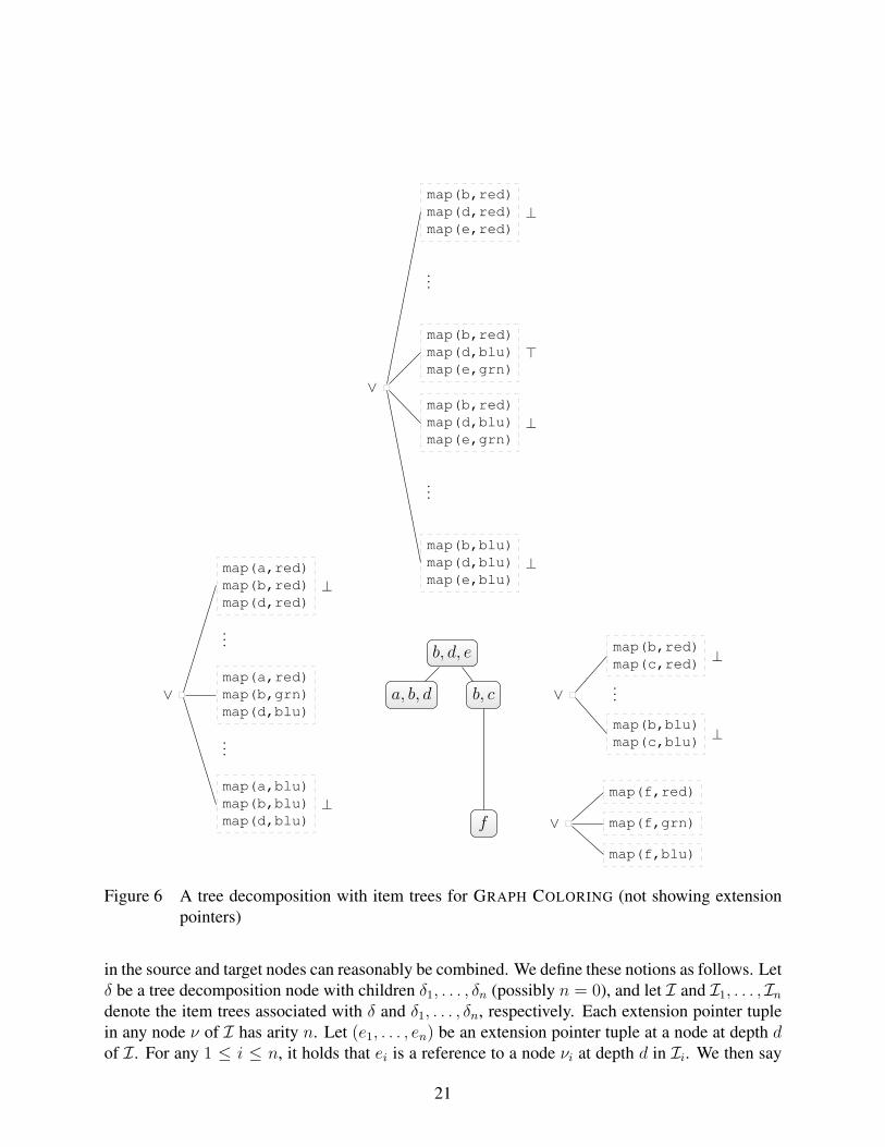
Example 2. Consider again the GRAPH COLORING instance from Example 1. Figure 6 shows atree decomposition for the input graph (Figure 1) and, for each decomposition node, the corre-sponding item tree that could result from an algorithm for GRAPH COLORING. For solving thisproblem, we use item trees having a height of at most 1. Each item tree node at depth 1 encodesa coloring of the vertices in the respective bag. The meaning of the symbols ∨, > and ⊥ will beexplained in Section 3.3.2.

3.3.1 Extension Pointers

In order to solve a complete problem instance, it is usually necessary to combine information fromdifferent item trees. For example, in order to find out if a proper coloring of a graph exists, we donot only have to check if a proper coloring of each subgraph induced by a bag exists but also if, foreach bag, we can pick a local coloring in such a way that each vertex is never colored differentlyby two chosen local colorings.

For this reason each item tree node has a (non-empty) set of extension pointer tuples. Theelements of such a tuple are called extension pointers and reference item tree nodes from childrenof the respective decomposition node. Roughly, an extension pointer specifies that the information

20

b, d, e

a, b, d b, c

f

∨

map(b,red)map(d,red)map(e,red)

⊥

...

map(b,red)map(d,blu)map(e,grn)

>

map(b,red)map(d,blu)map(e,grn)

⊥

...

map(b,blu)map(d,blu)map(e,blu)

⊥

∨

map(a,red)map(b,red)map(d,red)

⊥

...

map(a,red)map(b,grn)map(d,blu)

...

map(a,blu)map(b,blu)map(d,blu)

⊥

∨

map(b,red)map(c,red) ⊥

...

map(b,blu)map(c,blu) ⊥

∨

map(f,red)

map(f,grn)

map(f,blu)

Figure 6 A tree decomposition with item trees for GRAPH COLORING (not showing extensionpointers)

in the source and target nodes can reasonably be combined. We define these notions as follows. Letδ be a tree decomposition node with children δ1, . . . , δn (possibly n = 0), and let I and I1, . . . , Indenote the item trees associated with δ and δ1, . . . , δn, respectively. Each extension pointer tuplein any node ν of I has arity n. Let (e1, . . . , en) be an extension pointer tuple at a node at depth dof I. For any 1 ≤ i ≤ n, it holds that ei is a reference to a node νi at depth d in Ii. We then say

21

that ν extends νi.

Example 3. Consider Figure 6 again. In this example, we use the notation δS to denote thedecomposition node whose bag is the set S, and we write IS to denote the item tree of that node.

Although the figure does not depict extension pointers, we will explain how they would looklike in this example. In I{a,b,d} and I{f}, all nodes have the same set of extension pointer tuples:the set consisting of the empty tuple, as these decomposition nodes have no children.

In I{b,c}, the situation is more interesting: The root has a single unary extension pointer tuplewhose element references the root of I{f}. Each node at depth 1 of I{b,c} has three unary extensionpointer tuples – one for each node at depth 1 of I{f}.

The set of extension pointer tuples at the root of I{b,d,e} consists of a single binary tuple – oneelement references the root of I{a,b,d}, the other references the root of I{b,c}. For a node ν at depth 1of I{b,d,e}, the set of extension pointer tuples consists of all tuples (ν1, ν2) such that ν1 and ν2 arenodes at depth 1 of I{a,b,d} and I{b,c}, respectively.

3.3.2 Item Tree Node Types

Like states of ATMs, item tree nodes in D-FLAT can have one of the types “or”, “and”, “accept”or “reject”. Unlike ATMs, however, the mapping in D-FLAT is partial. The problem-specificalgorithm determines which item tree node is mapped to which type. The following conditionsmust be fulfilled.

• If a non-leaf node of an item tree has been mapped to a type, it is either “or” or “and”.

• If a leaf node of an item tree has been mapped to a type, it is either “accept” or “reject”.

• If an item tree node extends a node with defined type, it must be mapped to the same type.

When D-FLAT has finished processing all answer sets and has constructed the item tree for thecurrent tree decomposition node, it propagates information about the acceptance status of nodesupward in this item tree. This depends on the node types defined in this section, and is described inSection 3.5.2. The node types also play a role when solving optimization problems – roughly, whensomething is an “or” node, we would like find a child with minimum cost, and if something is an“and” node, we would like to find a child with maximum cost. This is described in Section 3.5.3.

Example 4. The item trees in Figure 6 all have roots of type “or”, denoted by the symbol ∨.This is because an ATM for deciding graph colorability starts in an “or” state, then guesses acoloring and accepts if this coloring is proper. Therefore, we shall derive the type “reject” in ourdecomposition-based algorithm whenever we determine that a guessed coloring is not proper, andwe derive “accept” once we are sure that a coloring is proper.7

In I{a,b,d} and I{f}, for instance, we have marked all leaves representing an improper coloringwith ⊥. The types of the other leaves are left undefined, as guesses on vertices that only appear

7It should be noted that the algorithm could be optimized by not even creating nodes encoding improper colorings.In order to remain faithful to the ATM analogy for the sake of presentation, we follow the habit of creating a branchfor each non-deterministic guess, even if this choice leads to a rejecting state.

22

later could still lead to an improper coloring. At the root of the tree decomposition however,we mark all item tree leaves having a yet undefined type with > because all vertices have beenencountered.

Note that it may happen that sibling nodes have equal item sets (like in I{b,d,e}). This is becausenodes with equal item sets but different types or counter values (cf. Section 3.7.2) are consideredunequal. Consider the two middle leaves in I{b,d,e}, for instance: The reason for one being markedwith > is that it extends only nodes whose type has still been undefined, whereas the leaf markedwith ⊥ extends at least one “reject” node.

3.3.3 Solution Costs for Optimization Problems

When solving an optimization problem with an ATM, we assume that with each accepting runwe can associate some kind of cost that depends on which non-deterministic choices have beenmade. Furthermore, we assume that the result of the ATM computation is now no longer “yes” or“no”, depending on whether the root of the computation tree is accepting or rejecting, but rather anumber that shall represent the optimum cost, for a certain notion of optimality that we will nowdefine.

For a non-deterministic Turing machine without alternation, the straightforward result of acomputation is the minimum cost among all runs. When alternation is involved, we can easilygeneralize this in the following way. Suppose each leaf of the computation tree is annotated with acost. (Rejecting nodes have cost∞.) The optimization value of a node ν can now be defined as (a)its cost if ν is a leaf, (b) the minimum cost among all children in case ν is an “or” node, and (c) themaximum cost among all children in case ν is an “and” node. The result of an ATM computationfor an optimization problem is then the optimization value of the root of its computation tree.

In analogy to this procedure of solving optimization problems, D-FLAT allows leaves of itemtrees to contain a number that specifies the cost that the respective branch has accumulated so far.That is, the cost that is stored in the leaf of an item tree refers not only to the non-deterministicchoices based on the current bag elements, but also on past choices (obtainable by following theextension pointers) from item trees further down in the decomposition.

3.4 D-FLAT’s Interface for ASPD-FLAT invokes an ASP solver at each node during a bottom-up traversal of the tree decompo-sition. The user-defined, problem-specific encoding is augmented with input facts describing thecurrent bag as well as the bags and item trees of child nodes. Additionally, the original probleminstance is supplied as input.8 The answer sets of this ASP call specify the item tree that D-FLATshall construct for the current decomposition node.

In Section 3.4.1 we describe the interface to the user’s ASP encoding, i.e., the input and outputpredicates that are used for communicating with D-FLAT. Note that there is also a simplified

8To be precise, D-FLAT provides the ASP system not with the whole problem instance but only with the part thatis induced by the current bag elements. This allows for fixed-parameter linear running time for decision and countingproblems. (Otherwise the same algorithms would be fixed-parameter quadratic.)

23

version of the ASP interface, which we describe in Section 3.4.2, for dealing with problems in NP.In all D-FLAT listings presented in this document, we use colors to highlight input and output

predicates.

3.4.1 General ASP Interface

D-FLAT provides facts about the tree decomposition as described in Table 1. Additionally, itdefines the integer constant numChildNodes to be the number of children of the current treedecomposition node. The item trees of these nodes are declared using predicates described inTable 2.

The answer sets of the problem-specific encoding together with this input give rise to the itemtree of the current tree decomposition node. Each answer set corresponds to a branch in the newitem tree. The predicates for specifying this branch are described in Table 3. We use the term“current branch” in the table to denote the branch that the respective answer set corresponds to;the “child item tree” shall denote an item tree that belongs to a child of the current tree decompo-sition node. One should keep in mind, however, that D-FLAT may merge subtrees as described inSection 3.5. Therefore, after merging, one branch in the item tree may comprise information frommultiple answer sets.

Example 5. A possible encoding for the GRAPH COLORING problem is shown in Listing 2. Notethat it makes more sense to encode this problem using the simplified ASP interface for problems inNP, which we describe in Section 3.4.2.

The first line in the listing is a modeline, which is explained in Section 3.8. Line 2 specifiesthat each answer set declares a branch of length 1, whose root node has the type “or”. Line 3guesses a color for each current vertex. The “reject” node type is derived in line 4 if this guessedcoloring is improper. Lines 5 and 6 guess a branch for each child item tree. Due to line 7, theguessed combination of predecessor branches only leads to an answer set if it does not contradictthe coloring guessed in line 3. This makes sure that only branches are joined that agree on allcommon vertices, as each vertex occurring in two child nodes must also appear in the current nodedue to the connectedness condition of tree decompositions. If a guessed predecessor branch hasled to a conflict (denoted by a “reject” node type), this information is retained in line 8.9 Finally,line 9 derives the “accept” node type if no conflict has occurred. The last two lines instruct theASP solver to only report facts with the listed output predicates, and we will justify their use laterin this section.

Note that some of the rules in Listing 2 can be used (with small modifications) for any problemthat is to be solved with D-FLAT. In particular, lines 5 and 6 are applicable to all problems afteradapting them to the item tree depth of the problem. Usually rules similar to line 3 are used forperforming a guess on bag elements (which of course depends on the problem), and checks aredone with rules similar to lines 4 and 7.

9Unless the user disables D-FLAT’s pruning of rejecting subtrees (cf. Section 3.5.2), this rule in fact never fires,but we list it anyway for a clearer presentation and to be consistent with the item trees in Figure 6.

24

Input predicate Meaning

initial The current tree decomposition node is a leaf.

final The current tree decomposition node is the root.

currentNode(N) N is the identifier of the current decomposition node.

childNode(N) N is a child of the current decomposition node.

bag(N, V ) V is contained in the bag of the decomposition node N .

current(V ) V is an element of the current bag.

introduced(V ) V is a current vertex but was in no child node’s bag.

removed(V ) V was in a child node’s bag but is not in the current one.

Table 1 Input predicates describing the tree decomposition

1 %d f l a t : −e v e r t e x −e edge – –no−empty−l e a v e s – –no−empty−r o o t2 length(1). or(0).3 1 { item(1,map(X,C)) : color(C) } 1 ← current(X).4 reject ← edge(X,Y), item(1,map(X,C;Y,C)).5 extend(0,S) ← rootOf(S,_).6 1 { extend(1,S) : sub(R,S) } 1 ← rootOf(R,_).7 ← item(1,map(X,C0)), childItem(S,map(X,C1)), extend(_,S), C0 6= C1.8 reject ← childReject(S), extend(_,S).9 accept ← final, not reject.

10 #show item/2. #show extend/2. #show length/1.11 #show or/1. #show accept/0. #show reject/0.

Listing 2 D-FLAT encoding for GRAPH COLORING using the general ASP interface

25

Input predicate Meaning

atLevel(S, L) S is a node at depth L of an item tree.

atNode(S,N) S is an item tree node belonging to decomposition node N .

root(S) S is the root of an item tree.

rootOf(S,N) S is the root of the item tree at decomposition node N .

leaf(S) S is a leaf of an item tree.

leafOf(S,N) S is a leaf of the item tree at decomposition node N .

sub(R, S) R is an item tree node with child S.

childItem(S, I) The item set of item tree node S contains I .

childAuxItem(S, I) The auxiliary item set (for the default join) of item tree nodeS contains I .

childCost(S,C) C is the cost value corresponding to the item tree leaf S.

childCounter(S, T, C) C is the counter value corresponding to the item tree leaf Sand the counter T .

childOr(S) The type of the item tree node S is “or”.

childAnd(S) The type of the item tree node S is “and”.

childAccept(S) The type of the item tree leaf S is “accept”.

childReject(S) The type of the item tree leaf S is “reject”.

Table 2 Input predicates describing item trees of child nodes in the decomposition

26

Output predicate Meaning

item(L, I) The item set of the node at level L of the current branchshall contain the item I .

auxItem(L, I) The auxiliary item set (for the default join) of the node atlevel L of the current branch shall contain the item I .

extend(L, S) The node at level L of the current branch shall extend thechild item tree node S.

cost(C) The leaf of the current branch shall have a cost value of C.

currentCost(C) The leaf of the current branch shall have a current cost valueof C.

counter(T,C) The counter T of the current branch shall have a value of C.

currentCounter(T,C) The current counter T of the current branch shall have avalue of C.

counterInc(T,C) The value of the counter T of the current branch shall beincreased by a value of C.

currentCounterInc(T,C) The value of the current counter T of the current branchshall be increased by a value of C.

counterRem(T ) The counter (and current counter) T of the current branchshall be removed.

length(L) The current branch shall have length L.

or(L) The node at level L of the current branch shall have type“or”.

and(L) The node at level L of the current branch shall have type“and”.

accept The leaf of the current branch shall have type “accept”.

reject The leaf of the current branch shall have type “reject”.

Table 3 Output predicates for constructing the item tree of the current decomposition node

27

Errors and Warnings. In order to support its users, D-FLAT issues errors and warnings to avoidunintended behavior. To list the most important ones, an error is raised if one of the followingconditions is violated.

• All output predicates from Table 3 are used with the correct arity.

• All atoms involving the extend/2 predicate refer to valid child item tree nodes.

• Each answer set contains exactly one atom involving length/1.

• Items, extension pointers or node types are placed at levels between 0 and the current branchlength.

• All extension pointer tuples specified in an answer set have arity n, where n is the numberof children in the decomposition.

• Items and auxiliary items are disjoint.

• Each extension pointer for level 0 points to the root of an item tree.

• Each extension pointer at level n+ 1 points to a child of an extended node at level n.

• All answer sets agree on the (auxiliary) item sets and extension pointers at level 0.

• If a node type is specified for a leaf, it is “or” or “and”.

• If a node type is specified for a non-leaf, it is “accept” or “reject”.

• A node is assigned at most one type.

• In the final decomposition node, each “and” and “or” node must have at least one child withdefined node type, or (in case such children have been pruned by D-FLAT) there must besome node reachable from that node via extension pointers that has a child with a definednode type.

• Only one (current) cost value is specified.

• Only one (current) counter value is specified for a certain first argument.

• Costs are specified only if all types of non-leaf nodes are defined.

• If in an answer set a currentCost/1 atom is contained, so must be an atom with cost/1.

• If in an answer set a currentCounter/2 atom is contained, so must be an atom withcounter/2, that has the same first argument as the former atom.

Furthermore, a warning is printed if one of the following conditions is violated.

28

• At least one #show statement occurs in the user’s encoding. (It should be used for perfor-mance reasons, and because D-FLAT can then check for specific #show statements, as de-scribed next. This is in order to check if the user has not forgotten about an output predicatethat is usually required for obtaining reasonable results.)

• A #show statement for length/1 occurs in the program.

• A #show statement for item/2 occurs in the program.

• A #show statement for extend/2 occurs in the program.

• A #show statement for or/1 or and/1 occurs in the program.

• A #show statement for accept/0 or reject/0 occurs in the program.

• All predicates used in a #show statement are recognized by D-FLAT.

3.4.2 Simplified Interface for Problems in NP

When dealing with problems in NP, the user of D-FLAT can choose to use a simpler interfacethan the one in Section 3.4.1. The reason for providing a second, less general, interface is that forproblems in that class it is usually sufficient to not use a tree-shaped data structure to store partialsolutions, but rather to use just a “one-dimensional” data structure: a table.

For instance, for the GRAPH COLORING problem we could just store a table at each tree de-composition node. Each row of such a table would then encode a coloring of the bag vertices.

Answer sets in D-FLAT’s table mode describe the rows of the current decomposition node’stable. A table is an item tree of height 1 where the root always has the type “or” and an empty itemset.10 Each item tree node at depth 1 corresponds to a row in the table. At the final decompositionnode, the type of each item tree node at level 1 is automatically set to “accept” by D-FLAT. Theuser therefore cannot (and does not need to) explicitly set item tree node types. Computationsleading to a rejecting state should – instead of deriving “reject” – simply not yield an answer set,which can be achieved by means of a constraint.

This way, algorithms for problems in NP can be achieved that are usually quite easy to read(and write).

The input predicates describing the decomposition are the same as in the general case, listed inTable 1. The input predicates declaring the child item trees (which we now call “child tables”) aredifferent, though, and described in Table 4. The output predicates specifying the current table arealso different in table mode. They are described in Table 5.

Example 6. The GRAPH COLORING problem admits a D-FLAT encoding using the simplified ASPinterface for problems in NP. A possible encoding using this table mode is shown in Listing 3.

10The case that tables in D-FLAT are empty cannot occur: As soon as a call to the ASP solver does not yield anyanswer sets (presumably because the respective part of the problem does not allows for a solution), D-FLAT terminatesand reports that no solutions exist.

29

1 %d f l a t : – – t a b l e s −e v e r t e x −e edge – –no−empty−l e a v e s – –no−empty−r o o t2 1 { extend(R) : childRow(R,N) } 1 ← childNode(N).3 item(map(X,C)) ← extend(R), childItem(R,map(X,C)), current(X).4 ← item(map(X,C0;X,C1)), C0 6= C1.5 1 { item(map(X,C)) : color(C) } 1 ← introduced(X).6 ← edge(X,Y), item(map(X,C;Y,C)).7 #show item/1. #show extend/1.

Listing 3 D-FLAT encoding for GRAPH COLORING using the table-mode ASP interface

Input predicate Meaning

childRow(R,N) R is a table row belonging to decomposition node N .

childItem(R, I) The item set of table row R contains I .

childAuxItem(R, I) The auxiliary item set (for the default join) of table row Rcontains I .

childCost(R,C) C is the cost value corresponding to the table row R.

childCounter(R, T, C) C is the counter value corresponding to the table row R andthe counter T .

Table 4 Input predicates (in table mode) describing tables of child nodes in the decomposition

30

Output predicate Meaning

item(I) The item set of the current table row shall contain the itemI .

auxItem(I) The auxiliary item set (for the default join) of the currenttable row shall contain the item I .

extend(R) The current table row shall extend the child table row R.

cost(C) The current table row shall have a cost value of C.

currentCost(C) The current table row shall have a current cost value of C.

counter(T,C) The counter T of the current table row shall have a value ofC.

currentCounter(T,C) The current counter T of the current table row shall have avalue of C.

counterInc(T,C) The value of the counter T of the current table row shall beincreased by a value of C.

currentCounterInc(T,C) The value of the current counter T of the current table rowshall be increased by a value of C.

counterRem(T ) The counter (and current counter) T of the current table rowshall be removed.

Table 5 Output predicates (in table mode) for constructing the table of the current decompositionnode

31

The first line differs from that in Listing 2 in the additional presence of the --tables optionto enable D-FLAT’s table-mode interface. Line 2 guesses a predecessor row whose coloring of thecurrent vertices is retained due to line 3. Line 4 makes sure that only compatible rows are joined.For the new vertices introduced into the current bag, line 5 guesses a coloring. The constraint inline 6 makes sure that the resulting coloring of the bag elements is proper. This way, each tablewill only contain rows that can be extended to proper colorings of the whole subgraph induced bythe current bag and all vertices from bags further down in the decomposition. Line 7 again makesthe ASP solver report only the relevant output predicates.

Some of the rules in Listing 3 are suited (after small adjustments) for any problem that is to besolved with D-FLAT in table mode. In particular, a rule like in line 2 is usually part of all table-mode encodings. Such encodings typically guess over the current vertices and then check that thisguess does not conflict with extended rows. Alternatively, as can be seen in the listing, it is oftenpossible to retain information from extended rows (line 3) and only guess on introduced vertices(line 5). In any case, it has to be made sure that the extended rows do not contradict each other orthe guessed information on the bag elements (line 4).

Errors and Warnings. In table mode, an error is raised if any of the following conditions isviolated:

• All output predicates from Table 5 are used with the correct arity.

• All atoms involving the extend/2 predicate refer to valid child item tree nodes.

• All extension pointer tuples specified in an answer set have arity n, where n is the numberof children in the decomposition.

• Items and auxiliary items are disjoint.

• Only one (current) cost value is specified.

• Only one (current) counter value is specified for a certain first argument.

• If in an answer set a currentCost/1 atom is contained, so must be an atom with cost/1.

• If in an answer set a currentCounter/2 atom is contained, so must be an atom withcounter/2, that has the same first argument as the former atom.

3.5 D-FLAT’s Handling of Item TreesEvery time the ASP solver reports an answer set of the user’s program for the current tree decom-position node, D-FLAT creates a new branch in the current item tree, which results in a so-calleduncompressed item tree. This step is described in Section 3.5.1. Subsequently D-FLAT prunessubtrees of that tree that can never be part of a solution, as described in Section 3.5.2, in orderto avoid unnecessary computations in future decomposition nodes. For optimization problems,

32

D-FLAT then propagates information about the optimization values upward in the uncompresseditem tree. This is described in Section 3.5.3. The item tree so far is called uncompressed becauseit may contain redundancies that are eliminated in the final step, as described in Section 3.5.4.

3.5.1 Constructing an Uncompressed Item Tree from the Answer Sets

In an answer set, all atoms using extend, item, or and and with the same depth argument, aswell as accept and reject, constitute what we call a node specification. To determine wherebranches from different answer sets diverge, D-FLAT uses the following recursive condition: Twonode specifications coincide (i.e., describe the same item tree node) iff

1. they are at the same depth in the item tree,

2. their item sets, counter values (for leaf nodes) – if specified, extension pointers and nodetypes (“and”, “or”, “accept” or “reject”) are equal, and

3. both are at depth 0, or their parent node specifications coincide.

In this way, an (uncompressed) item tree is obtained from the answer sets.

3.5.2 Propagation of Acceptance Statuses and Pruning of Item Trees

In Section 3.3.2 we have defined the different node types that an item tree node can have (“un-defined”, “or”, “and”, “accept” and “reject”). When D-FLAT has processed all answer sets andconstructed the uncompressed item tree, these types come into play. That is to say, D-FLAT thenprunes subtrees from the uncompressed item tree.

First of all, if the current tree decomposition node is the root, D-FLAT prunes from the uncom-pressed item tree any subtree rooted at a node whose type is still undefined.11 Then, regardless ofwhether the current decomposition node is the root, D-FLAT prunes subtrees of the uncompresseditem tree depending on the acceptance status of its nodes. The acceptance status of a node caneither be “undefined”, “accepting” or “rejecting”, which we define now.

A node in an item tree is accepting if (a) its type is “accept”, (b) its type is “or” and it hasan accepting child, or (c) its type is “and” and all children are accepting. A node is rejecting if(a) its type is “reject”, (b) its type is “or” and all children are rejecting, or (c) its type is “and” andit has a rejecting child. Nodes that are neither accepting nor rejecting are said to have an undefinedacceptance status.

After having computed the acceptance status of all nodes in the current item tree, D-FLATprunes all subtrees rooted at a rejecting node, as we can be sure that these nodes will never be partof a solution.

Note that in case the current decomposition node is the root, there are no nodes with undefinedacceptance status because D-FLAT has pruned all subtrees rooted at nodes with undefined type.Therefore, in this case, the remaining tree consists only of accepting nodes. For decision problems,

11In order to keep the semantics meaningful, D-FLAT issues an error if an “and” or “or” node has only childrenwith undefined type in the final decomposition node. It is the responsibility of the user to exclude such situations.

33

we can thus conclude that the problem instance is positive iff the remaining tree is non-empty.For enumeration problems, we can follow the extension pointers down to the leaves of the treedecomposition in order to obtain complete solutions by combining all item sets and counter values(for leaf nodes) – if specified – along the way. This is described in more detail in Section 3.6.Recursively extending all item sets in this way would yield a (generally very big) item tree thatusually corresponds to the accepting part of a computation tree that an ATM would have whensolving the complete problem instance. (But of course D-FLAT does not materialize this tree inmemory.)

Example 7. Consider again Figure 6. Because I{b,d,e} is the final item tree in the decompositiontraversal, D-FLAT would subsequently remove all nodes with undefined types (but there are nonein this case). Then it would prune all rejecting nodes and conclude that the root of I{b,d,e} isaccepting because it has an accepting child. Therefore the problem instance is positive. At thedecomposition root, we are then left with an item tree having only three leaves, each encoding aproper coloring of the vertices b, d and e, and storing extension pointers that let us extend therespective coloring for these vertices to proper colorings on all the other vertices, too.

3.5.3 Propagation of Optimization Values in Item Trees

For optimization problems, after an uncompressed item tree has been computed, an additionalstep is done in addition to what we described in Section 3.5.2. Each leaf in the item tree storesan optimization value (or “cost”) that has been specified by the user’s program. D-FLAT nowpropagates these optimization values from the leaves toward the root of the current uncompresseditem tree in the following way:

• The optimization value of a leaf node is its cost.

• The optimization value of an “or” node is the minimum among the optimization values of itschildren.

• The optimization value of an “and” node is the maximum among the optimization values ofits children.

Note that D-FLAT currently raises an error if costs are specified for a leaf that has some ancestorwith undefined node type.

3.5.4 Compressing the Item Tree

The uncompressed item tree obtained in the previous step may contain redundancies that must beeliminated in order to avoid an explosion of memory and runtime. The following two situationscan arise where D-FLAT eliminates redundancies:

• There are two isomorphic sibling subtrees where all corresponding nodes have equal itemsets, counter values (for leaf nodes), node types and (when solving an optimization problem)optimization values.

34

In this case, D-FLAT merges these subtrees into one and unifies their sets of extension point-ers.

• An optimization problem is being solved and there are two isomorphic sibling subtrees whereall corresponding nodes have equal item sets, counter values (for leaf nodes) – if specified –and node types, but the root of one of these sibling subtrees is “better” than the root of theother subtree. In this context, a node n1 is “better” than one of its siblings, n2, if the parentof n1 and n2 either has type “or” and the cost of n1 is less than that of n2, or their parent hastype “and” and the cost of n1 is greater than that of n2.

In this case, D-FLAT retains only the subtree rooted at the “better” node.

Note that in table mode this redundancy elimination can be done on the fly. That is, every timean answer set is reported, it can be detected right away if this leads to a new table row or if a tablerow with the same item set and the same counter values – if specified – already exists. This way,D-FLAT does not need to build an uncompressed item tree that can only be compressed once allanswer sets have been processed. However, if item trees have a height greater than 1, this is notpossible, as multiple answer sets constitute a subtree in general.

3.6 Materializing Complete SolutionsAfter all item trees have been computed, it remains to materialize complete solutions. We firstdescribe how D-FLAT does this in the case of enumeration problems.

In the item tree at the root of the decomposition there are only accepting nodes left after thepruning described in Section 3.5.4. Starting with the root of this item tree, D-FLAT extends eachof the nodes recursively by following the extension pointers, as we will describe next.

To obtain a complete extension of an item tree rooted at a node n, we first pick one of theextension pointer tuples of n. We then extend the item set of n by unifying it with all items in thenodes referenced by these extension pointers. Then we again pick one extension pointer tuple foreach of the nodes that we have just used for extending n and repeat this procedure until we havereached a leaf of the tree decomposition. This gives us one of the possible extensions of n. Foreach of the children of n we also perform this procedure and add all possible extensions of thatchild to the list of children of the current extension of n. When extending a node m with parent nin this way, however, D-FLAT takes care to only pick an extension pointer tuple of m if every nodethat is being pointed to in this tuple is a child of a node that is used for the current extension of n.

When an optimization problem is to be solved, D-FLAT only materializes optimal solutions.That is, if n is an “or” node with optimization value c, D-FLAT only extends those children of nthat actually have cost c. This is because, due to D-FLAT’s propagation of optimization values (cf.Section 3.5.3), the optimization value of an “or” node is the minimum of the optimization valuesof its children. For “and” nodes this is symmetric.

D-FLAT allows the depth until which the final item tree is to be extended to be limited bythe user. This is useful if, e.g., only existence of a solution shall be determined. In such a case,we could limit the materialization depth to 0. This would lead to only the root of the final itemtree being extended. If D-FLAT yields an extension, a solution in fact exists. This is because

35

the final item tree would have no root in case no solutions existed (cf. Section 3.5.4). Limitingthe materialization depth in this case saves us from potentially materializing exponentially manysolutions when all we are only interested in knowing if there is a solution.

Moreover, limiting the materialization depth is also helpful for counting problems. If the userlimits this depth to d and in the final item tree there is a node at depth d having children, D-FLATprints for each extension of this node how many extended children would have been materialized.This behavior can be disabled to increase performance, but for the most common case, wherethe materialization depth is limited to 0, it is not required to disable this feature. The reason isthat in such cases D-FLAT is able to calculate the number of possible extensions while doing themain bottom-up traversal of the decomposition for computing the item trees. Hence, for classicalcounting problems, D-FLAT offers quite efficient counting.

3.7 Further Functionality3.7.1 Default Join

In weakly normalized, semi-normalized and normalized tree decompositions, nodes with morethan one child are called join nodes. Such nodes have the same bag as each of its children (cf.Section 3.2). For join nodes, D-FLAT offers a default implementation for computing the item tree.

This default join implementation combines the item trees from the child nodes in the followingway. For each child node, an item tree branch is selected such that for each pair of selected branchesand each pair of nodes at the same depth in these branches it holds that the item sets, counter values(for leaf nodes) – if specified – and node types are equal. This is done for all possible combinationsof item tree branches.

Once D-FLAT finds a combination of joinable branches, it inserts a branch whose item sets andcounter values – if specified – are equal to those of the selected branches into the new item tree. Incase costs (or counters) have been specified, D-FLAT first sets the cost (or the values of the speci-fied counters) of this new branch to the sum of costs of the selected predecessors, but – similar tothe inclusion-exclusion principle – costs (or counter values) that have been counted multiple timesmust be subtracted. This is why D-FLAT recognizes the output predicate currentCost/1 (andcurrentCounter/2, currentCounterInc/3+, (cf. Section 3.7.2)), which is used for quantify-ing the part of the cost (or counter), specified by cost/1 (or counter/2, counterInc/3+), thatis due to current bag elements. If there are n child nodes in the decomposition, D-FLAT subtractsn−1 times the current cost (or counter) value from the sum of the predecessor costs (or counters).12

Example 8. Consider again the GRAPH COLORING problem and the encoding from Listing 3.Suppose we only want to consider weakly normalized decompositions (or even stronger forms ofnormalizations) and use the default join implementation for all nodes with more than one child.Then we could remove line 4 from Listing 3 because the default join takes care of only combiningitem tree nodes (i.e., in this case, table rows) with equal item sets. The resulting encoding incombination with the default join would always yield the same results as Listing 3.

12D-FLAT assumes that equality of item sets implies the same current cost (or counter) value, so each branch in ajoinable combination features the same current cost (or counter) value.

36

Sometimes it is desired to join two branches even though they only agree on some part of thecontained information. That is, we would like to express that some items are critical in determiningwhether two branches are joinable while some other items are irrelevant for this because they aresome kind of auxiliary information.

For such situations, D-FLAT offers the possibility of using auxiliary items. Every item treenode thus contains, beside the ordinary item set, an auxiliary item set (that is disjoint from theordinary one). Whenever we want to store an item in a node without preventing this node to bejoined with nodes that do not contain this item, we can declare it as an auxiliary item. D-FLATjoins two branches even if their auxiliary item sets are different as long as their ordinary item sets,counter values – if specified – and item tree node types are equal. The auxiliary item sets in thebranch resulting from the join is then set to the union of the respective auxiliary item sets of thenodes of the joined branches. For an example, see Section 4.3.

The same behavior could also be achieved in an ASP program. The default join implementationis, however, much more efficient than using an ASP solver. Firstly, of course the default joinimplies less overhead as it is implemented directly in D-FLAT using C++. Secondly, it can makeuse of the fact that D-FLAT stores item trees using a certain order that allows for very quick joining.This is similar to the sort-merge join algorithm in relational database management systems.

3.7.2 Built-in Counters

Starting with version 1.2.0, D-FLAT offers also so-called counters [2], which extend the func-tionality offered for tracking the cost of each solution to any kind of counter, and with which theuser can outsource certain computations from ASP to D-FLAT. Keeping track of costs or otherelements which need to be counted no longer requires using aggregate functions, leading to am-ple groundings and long run-times. Instead, D-FLAT offers the means to store the value for anydefined counter, not only for the cost of a solution and also to increment these values instead ofrecalculating them in every ASP call.

First, the user can utilize the output predicates counter/2 and currentCounter/2, whichboth take a string and an integer value as parameters. The first sets the value of the counter denom-inated by the first argument, in the current table row, or the leaf of the current branch, respectively.If a counter with this denomination does not exist yet, it is first created. The second is needed whenusing the option --default-join and sets only the value of the counter corresponding to thecurrent node, in order to be used by D-FLAT when applying the inclusion-exclusion principle toautomatically merge counter values from different branches at join nodes. The use of these twopredicates enhances higher readability and maintainability of the code and makes post-processingnodes with identical bag elements above the join node superfluous. For the user to be able tocompute counter values in the current node, the input predicate childCounter/3 is printed foreach counter, at each node of the tree decomposition, and passed as input for the parent node. Itsarguments are the extended table row of the child node, or the extended item tree leaf of the childnode, respectively, the denomination of the counter, and its value.

Further, D-FLAT offers the output predicates counterInc/3+ and currentCounterInc/3+,which can be used alternatively to counter/2 and currentCounter/2. With the former we can

37

specify via its second argument by how much a certain counter or current counter denominated bythe first argument will be incremented (or decremented, when using negative values). The values tobe incremented are taken by D-FLAT from the extended table row in the child node, or the extendeditem tree leaf in the child node, respectively. The rest of the arguments is used to make eachinstantiation of the predicate unique and their number depends on how many of them are neededfor this purpose. Again, if the counter does not exist yet, it is created with the first occurrence ofthe predicate counterInc/3+. Using these predicates improves run-time dramatically in average,as they make the use of aggregate functions superfluous for keeping track of counters, otherwisehaving their values computed in ASP at every node of the tree decomposition or even handledusing items. The greater the values of the counters are, the higher is the gain in running time.

For removing counters which will not be necessary anymore, D-FLAT provides the outputpredicate counterRem/1, whose argument is the denomination of the counter to be removed.Further, when the denomination of the counter is “cost”, it acts as a cost declaration and D-FLAToptimizes the set of solutions specifically on the values stored in this counter. Further, if countersother than the one denominated by “cost” have different values for identical items sets, the partialanswer sets are not merged and the counters are printed as if they were items. However, whenusing the option --default-join, the merge of different table rows is not done on the equalityof counters, which are in fact recalculated based on the values in the child nodes and the currentcounter value. In this way, counters work rather like auxiliary items. For performance results onusing built-in counters, please refer to [2]. Examples illustrating the use of built-counters can befound in Section 4.4.

3.7.3 Lazy Evaluation

Starting with version 1.2.0, D-FLAT also puts an implementation for “lazy” dynamic program-ming [14] at the user’s disposal, when working in table mode. When the user opts for lazy eval-uation by specifying the option --lazy, D-FLAT does not compute every row of a table beforeadvancing to the next node of the tree decomposition but rather tries to deliver solutions by com-puting as few table rows as possible: Whenever a new row r is inserted into a table T , D-FLATtries to extend r to a new row in the parent table. A new row is computed at T if all attempts ofextending r have failed. Thus, in the best case, only one row per table needs to be computed inorder to find a solution. By default, D-FLAT uses an ASP technology called “multi-shot solving”in order to avoid invoking the grounder whenever a new row has been computed. The user mayturn off this behavior (with the option --reground), but experiments showed regrounding to beclearly less efficient. Lazy evaluation is especially useful for optimization problems. It may notonly lead to better performance but also allows for anytime computations, that is, the possibilityto abort the execution at any point and report the best solution found so far. The user may specifythe option --print-provisional, which prints solutions that improve the current optimumas they are found.

Next, we will outline how lazy evaluation works on the whole.13 D-FLAT runs many ASPsystems in parallel – one for each tree decomposition node. These interact during the lazy evalua-

13For the detailed algorithms behind, please refer to [14].

38

tion, as we will describe in the following. After D-FLAT has constructed a tree decomposition, itrequests a row from the root node. This triggers a recursion as follows:

When a leaf node is requested to produce a new row, its ASP solver is asked to find the nextanswer set (or, in the beginning, the first one). If this is impossible, the leaf reports that it isexhausted, that is, no new rows can be produced at its table.

When an exchange node is requested to produce a new row but the child table is empty, it firstasks its child to produce a row. Then the exchange node invokes its ASP solver in order to computea row at its own table by extending that child row. If this is impossible, it asks its child for the nextrow and repeats this process until it can produce a row. Subsequently, whenever the exchange nodeis requested to produce a new row, it first tries to obtain a new answer set from the last computedchild row, and if this fails it asks the child for a new row. If at any point the child is exhausted, theexchange node is also exhausted.

For join nodes, the same idea is extended to more than one child. Here, D-FLAT first tries outall combinations of existing child rows and tries to compute a new row extending that combination.Only when all possible such combinations have been considered, a new row is requested fromone of the child nodes in a round-robin fashion: A child node is only asked to produce a newrow when all other nodes have been asked before (or are already exhausted). D-FLAT followsthis round-robin strategy in the hope of obtaining solutions more quickly than by filling one childtable completely before proceeding to the next one. Once a child table comes up with a new row,D-FLAT iterates over all combinations of this new row with existing rows of the other child nodes.For each such combination, the join node invokes its ASP solver in order to find all rows thatextend that combination.

D-FLAT’s lazy mode also incorporates some more optimizations that can be deactivated by theuser if wanted. First, when working with the default join, D-FLAT keeps tables sorted; now when-ever a child produces a new row, D-FLAT uses binary search in order to quickly find matching rowsthat already exist in the tables of the other children. By using the option --no-binary-searchthe user can deactivate this binary search and instead have all combinations be tried out sequen-tially. (Experiments showed, however, that binary search usually gives better performance.) Sec-ond, when solving optimization problems, D-FLAT uses the branch-and-bound strategy by default,in order to reject partial solution candidates that will for sure lead to solutions that are more expen-sive than the best solution found so far. For this, D-FLAT carries a global variable, which containsthe cost of the best solution found so far. A newly found row candidate is inserted into a tableonly if its cost does not exceed this upper bound. If only this simple branch-and-bound procedureis wanted, it can be indicated using the option --bb basic. By default, however, D-FLAT im-plements a refined branch-and-bound strategy, which not only discards solution candidates whentheir cost exceeds the cost of the best solution so far, but it also tries to determine lower boundsand uses these for finding better upper bounds as follows: Suppose that node n has children n1

and n2, and that n1 is exhausted, which intuitively means that we “know everything” about thesubgraph induced by the vertices that have been forgotten up to n1 (i.e., they appear in a bag of anode below n1 but not in the bag of n1 itself). Suppose further that c is the minimum cost of allpartial solutions of the latter subgraph. Then, we can reject a candidate row at n2 already whenits cost exceeds k − c, where k is the cost of the best solution so far. This behavior is explicitly

39

chosen with the option --bb full and it is in fact the default. For the case that the user dealswith a problem that does not exhibit monotone costs (i.e., the cost of a row is possibly lower thanthe sum of the costs of the rows it extends), the option --bb none turns off branch and bound.

As grounding is done only once at each node before having any information from rowsin child tables, the user must declare atoms that pass on information from child rows (i.e.,childItem/1, childAuxItem/1, childCost/1, childCounter/2 atoms) as #external in or-der for the grounder not to assume these atoms to be false even though they cannot be derived byany rule. Each time the ASP solver is called, the truth values of these atoms are temporarily frozenaccording to the child rows currently considered. Note that the arity of the former predicates issmaller than in the normal “eager” mode of D-FLAT. The reason is that the first argument, whichwould denote a child row in eager mode, is omitted in lazy mode. Moreover, the extend/1 predi-cate is not used at all in lazy mode. The reason is that D-FLAT now invokes the ASP solver oncefor every combination of child rows (instead of once per tree decomposition node), so it is alreadyclear which combination of child rows is to be extended. Starting with version 1.2.5, D-FLAT’slazy evaluation mode also supports built-in counters and optimization on costs declared by theuser. An example of such an encoding is provided in Section 4.5.

3.8 Command-Line UsageIn this section we present how D-FLAT can be used from the command line.

General Options

• -h: Print usage information and exit.

• --version: Print version number and exit.

• -p <program>: Use <program> as the ASP encoding that is to be called at each treedecomposition node. This option may be used multiple times, in which case all specifiedprograms are jointly used.

• -e <edge>: Predicate <edge> declares (hyper)edges in the input facts.(This is explained in Section 3.2.)

• -f <file>: Read the problem instance from <file>. By default, standard input is used.

• --seed <n>: Initialize the random number generator with seed <n>.

• --tables: Use the table mode described in Section 3.4.2, i.e., the simplified ASP interfacewhen a table suffices for storing problem-specific data. If this option is absent, D-FLAT usesthe general interface described in Section 3.4.1.

• --ignore-modelines: Do not scan the encoding files for modelines, which are ex-plained below.

40

• --stats: Print Clasp statistics.

• --default-join: Use the built-in default implementation for join nodes instead of in-voking the ASP solver there. This is described in Section 3.7.1.

Options for Constructing a Tree Decomposition

• -d <decomposer>: Use decomposition method <decomposer>, which is one of thefollowing.

– dummy: Do not decompose (place all vertices into only one node).

– td: Create a tree decomposition using bucket elimination. (This is the default.)

– graphml: Use the decomposition specified in the GraphML file provided by the user.

• -n <normalization>: Use the normal form <normalization>, which is one of thefollowing.

– none: No normalization. (This is the default.)

– weak: Weak normalization.

– semi: Semi-normalization.

– normalized: Normalization.

• --elimination <h>: Use the heuristic <h> for the bucket elimination algorithm. Thefollowing values are supported.

– min-degree: Minimum degree ordering. (This is the default.)

– min-fill: Minimum fill ordering.

• --fitness <criterion>: From several generated tree decompositions, choose theone with the <criterion> with the minimal value, where <criterion> can be one ofthe following.

– width: Maximum bag size. (This is the default.)

– join-bag-avg: Average join node bag size (defaulting to 0 if there is no join nodein the tree decomposition).

– join-bag-median: Median join node bag size (defaulting to 0 if there is no joinnode in the tree decomposition).

– num-joins: Number of join nodes.

• --iteration-count <i>: Use <i> iterations for finding the fittest tree decomposi-tion. (The default value is 1.)

The decomposition strategies mentioned above are briefly described in Section 3.2.

41

• --no-empty-root: By default, D-FLAT constructs tree decompositions with an emptybag at the root. This option disables that behavior.

• --no-empty-leaves: By default, D-FLAT constructs tree decompositions with anempty bag at every leaf. This option disables that behavior.

• --post-join: Tree decompositions contain above each join node a parent node with iden-tical bag. This can be useful especially when using default join and some post-processingneeds to be done on the bag elements of the join node after merging them.

• --path-decomposition: Generate a path decomposition, which is a tree decomposi-tion that does not contain any join nodes.

Solving Options

• -s <solver>: In order to compute partial solutions, use <solver>, which is one of thefollowing.

– dummy: Do not perform solving and always report the empty item tree.

– clasp: Use Answer Set Programming solver Clasp. (This is the default.)

• --no-optimization: Do not optimize on costs.

• --cardinality-cost: Use item set cardinality as costs.

• --depth <d>: Limit materialization of final item tree to <d>.(This is explained in Section 3.6.)

• --no-counting: Do not count the number of solutions.

• --no-pruning: Prune rejecting subtrees only in the decomposition root (for instance fordebugging).

Printing Options

• --print-decomposition: Print the generated decomposition.

• --output <module>: Print information during the run using <module>, which is oneof the following.

– quiet: Only print the final result of the computation.

– progress: Print a progress report. (This is the default.)

– human: Human-readable debugging output.

42

– machine: Machine-readable debugging output that includes information about ex-tension pointers (for instance for a debugging tool such as the D-FLAT Debugger forD-FLAT version 1.1.0, as described in [1]).

– count-rows: Print the number of level-1 item tree nodes (or rows in table mode) foreach decomposition node.

• --print-solver-events: Print events occurred during solving (for instance findinganswer sets).

• --print-solver-events: Print the input passed on to the solver on its invocation.

• --print-uncompressed: Print item trees before compression. The mechanism for thelatter is described in Section 3.5.4.

Options for Using the GraphML Format

• --graphml-in <file>: Read the decomposition in GraphML format from <file>.

• --graphml-out <file>: Write the decomposition in the GraphML format to<file>.

• --add-empty-root: When using a decomposition read in GraphML format from a file,add an empty root to it.

• --add-empty-leaves: When using a decomposition read in GraphML format from afile, add empty leaves to it.

Options for Lazy Evaluation

• --lazy: When in table mode, use lazy evaluation to find at least one solution. This isdescribed in Section 3.7.3.

• --no-binary-search: Disable binary search on table rows to be matched at join nodeswhen using default join and lazy evaluation.

• --bb <s>: Using branch and bound strategy <s> when using lazy evaluation and optimiz-ing on costs. The following values are permitted.

– none: Do not use branch and bound.

– basic: Prevent rows not cheaper then the current provisional solution.

– full: Improve bounds for partial solution costs by using optimal cost values of partialsolutions for forgotten subgraphs. (This is the default.)

• --print-provisional: Report possibly non-optimal solutions before determining theoptimal solution(s) when using lazy evaluation (for instance when stopping the computationafter a fixed amount of time).

43

• --reground: Reground every time a row is passed on from a child node instead of usingexternal atoms when using lazy evaluation.

Modelines Usually a D-FLAT encoding only produces meaningful results if it is used in combi-nation with certain command-line options. For instance, usually an encoding relies on a specificname of the (hyper)edge predicate or maybe a certain normalization of the tree decomposition.Because it is tedious to always specify these options, D-FLAT supports so-called modelines in theASP encodings.

D-FLAT scans the first line of each encoding specified via -p. If this line starts with %dflat:(followed by a space), the rest of the line is treated as if it were supplied to the command line.

For instance, an encoding that requires the table mode ASP interface (cf. Section 3.4.2), semi-normalized tree decompositions and an edge predicate called edge (as well as vertex for in-cluding isolated vertices in the decomposition – cf. Section 3.2), might start with the followingmodeline.

1 %d f l a t : – – t a b l e s −e v e r t e x −e edge −n semi

This way, D-FLAT only needs to be called with -p together with the encoding’s filename.

44

4 D-FLAT in PracticeIn this section we illustrate the applicability of D-FLAT to different types of computational prob-lems. We will exemplify its functionality upon encodings of different variants of the DOMINATING

SET problem, which we also refered to in Section 2.2.2. In Section 4.1 encodings for some vari-ants of the problem in NP are described in detail. The same is done in Section 4.2 for a variantharder than NP. In Sections 4.3, 4.4, and 4.5 we illustrate how to use default join, built-in countersand lazy evaluation, using furhter D-FLAT encodings. Note that for actually running these encod-ings, #show statements should be added in order to avoid getting a warning (cf. Section 3.4). Weomitted these statements for the sake of brevity.

For implementations of further problems in NP, as well as beyond NP, please refer to thefirst Progress Report from 2014 [1] and the project website14. There you can find also ecod-ings for the enumeration counterparts of NP-hard problems, such as MINIMUM VERTEX COVER,NP-complete problems like SAT, FEEDBACK VERTEX SET, HAMILTONIAN CYCLE, INDE-PENDENT SET, MAXIMUM CUT, ODD CYCLE TRANSVERSAL, STEINER TREE, and evenΣP

2 -complete problems such as SECURE SET or ⊆-MINIMAL SAT, and PSPACE-complete ones,like QSAT and MSO MODEL CHECKING.

4.1 Problems in NP4.1.1 Minimum Dominating Set

Input: An undirected graph G = (V,E).

Task: Compute all cardinality-minimal dominating sets of G. A subset X of V is adominating set of G if for each v ∈ V the vertex is part of X or v is adjacent toat least one u ∈ X (i.e. is dominated by at least one u ∈ X).

ASP allows a very succinct modeling of the problem and also formulating it for D-FLAT yieldsa very simple encoding. The encoding (see Listing 4) represents one possibility of how to en-code the optimization variant of DOMINATING SET in D-FLAT and implements a simple Guess& Check approach, following the ideas of the dynamic programming algorithm we introduced inSection 2.2.2. The code defines the recipe of how the information has to be handled in a node of thetree decomposition. We have to guess rows to be extended (line 5) and check whether these rowscoincide on vertices contained in the dominating set (line 7). Information contained in a child rowhas to be retained in case that the corresponding vertex is still present in the current decompositionnode (lines 9–10). In case a vertex is removed that is neither selected nor dominated, the respectivesolution candidate is discarded (line 12). For each introduced vertex we guess if it is selected to bepart of a dominating set (line 14), and we derive which vertices are now dominated (line 16).

Up to now, there is no optimization involved. This task is done by employing the outputpredicate cost/1 in lines 17–22 of the encoding. For leaf nodes, the cost simply coincides with

14See http://dbai.tuwien.ac.at/research/project/dflat/system/examples/encodings-dbai-tr-2017-107.tar.gz

45

1 % Make e x p l i c i t t h a t edges a r e u n d i r e c t e d .2 edge(X,Y) ← current(X;Y), edge(Y,X).

3 % Make e x p l i c i t t h a t a v e r t e x i s n o t s e l e c t e d i n a row .4 out(R,X) ← childRow(R,N), bag(N,X), not childItem(R,sel(X)).

5 1 { extend(R) : childRow(R,N) } 1 ← childNode(N).

6 % Only j o i n rows t h a t c o i n c i d e on s e l e c t e d v e r t i c e s .7 ← extend(R1;R2), childItem(R1,sel(X)), out(R2,X).

8 % R e t a i n r e l e v a n t i n f o r m a t i o n .9 item(sel(X)) ← extend(R), childItem(R,sel(X)), current(X).

10 item(dom(X)) ← extend(R), childItem(R,dom(X)), current(X).

11 % Ensure t h a t removed v e r t i c e s a r e s e l e c t e d o r domina ted .12 ← removed(X), extend(R), not childItem(R,sel(X)), not childItem(R,dom(X)).

13 % Guess s e l e c t e d v e r t i c e s .14 { item(sel(X)) : introduced(X) }.

15 % A v e r t e x i s domina ted i f i t i s a d j a c e n t t o a s e l e c t e d v e r t e x .16 item(dom(Y)) ← item(sel(X)), edge(X,Y), current(X;Y).

17 % Leaf node c o s t s .18 cost(NC) ← NC = #count{ X : item(sel(X)) }, initial.19 % Exchange node c o s t s .20 cost(CC + NC) ← extend(R), childCost(R,CC),

NC = #count{ X : item(sel(X)), introduced(X) }, numChildNodes == 1.21 % J o i n node c o s t s .22 cost(CC - (LC * (EP - 1))) ← CC = #sum { C,R : extend(R), childCost(R,C) },

LC = #count { X : item(sel(X)) }, EP = numChildNodes, EP >= 2.

Listing 4 D-FLAT encoding for MINIMUM DOMINATING SET

46

the number of selected vertices. For exchange nodes we add the number of selected introducedvertices to the extended child row’s cost. For join nodes we have to compute the sum of all thechild rows’ costs and subtract numChildNodes−1 times the current costs following the inclusion-exclusion principle. Note that we require the tree decomposition to be weakly normalized, as weassume in our cost function that the bag of a join node coincides with the bags of its child nodes.

Further note that this encoding only requires item trees of height 1, which allows for theuse of the table-based D-FLAT interface. As described in Section 3.4.2, the input predicateschildNode/1, childRow/2 specify the child nodes in the decomposition and the rows in theirtables, and current/1, introduced/1 and removed/1 denote the vertices that are in the cur-rent bag, have been newly introduced in it or have appeared in a child node’s bag but no longer arecontained in the current bag, respectively. The output predicate item/1 (and auxItem/1) definesthe (auxiliary) item set of the current row, and cost/1 defines the cost value of the current row.extend/1 determines for each child node the row to be extended by the current row. The inputpredicates childItem/2 (and childAuxItem/2), childCost/2 specify the item sets (and aux-iliary item sets) of the child nodes and their cost values. initial/0 denotes that the current nodeis a leaf and numChildNodes/0 denotes the number of children of the current node.

4.1.2 Connected Dominating Set

Input: An undirected graph G = (V,E).

Task: Compute all connected dominating sets of G. A subset X of V is a connecteddominating set of G if the sub-graph G′ of G induced by X is connected andfor each v ∈ V the vertex is part of X or v is adjacent to at least one u ∈ X .

As seen before, D-FLAT allows one to implement dynamic programming algorithms in a verysuccinct way. To underline that D-FLAT is also suitable for solving problems where the inter-nal data structure, i.e., the information that is propagated through the decomposition nodes, ismore complicated, we show how the CONNECTED DOMINATING SET problem can be solved withD-FLAT.

The encoding is given in Listing 5. Observe that lines 1–16 are the same as in the encodingfor MINIMUM DOMINATING SET. We additionally use the function symbols stop/0, con/2 andest/2. For any pair of selected vertices, con/2 is derived if the vertices are connected (lines 18–20), while predicate est/2 denotes that there has not been any evidence of their connectedness yet(lines 22–23). Once a vertex x is removed, we check if x still needs to be connected to anotherselected vertex y in the current bag and if no connection to another selected vertex z in the currentbag exists, the solution candidate is eliminated (line 24).

To avoid solutions containing isolated components, we denote by the function symbol stop/0that the last selected vertex is removed from the bag (line 28). We then remove every solutioncandidate where a new vertex is introduced after stop was derived (line 29) or two rows are to bejoined that both contain stop (line 30).

47

1 % Make e x p l i c i t t h a t edges a r e u n d i r e c t e d .2 edge(X,Y) ← current(X;Y), edge(Y,X).

3 % Make e x p l i c i t t h a t a v e r t e x i s n o t s e l e c t e d i n a row .4 out(R,X) ← childRow(R,N), bag(N,X), not childItem(R,sel(X)).

5 1 { extend(R) : childRow(R,N) } 1 ← childNode(N).

6 % Only j o i n rows t h a t c o i n c i d e on s e l e c t e d v e r t i c e s .7 ← extend(R1;R2), childItem(R1,sel(X)), out(R2,X).

8 % R e t a i n r e l e v a n t i n f o r m a t i o n .9 item(sel(X)) ← current(X), extend(R), childItem(R,sel(X)).

10 item(dom(X)) ← current(X), extend(R), childItem(R,dom(X)).

11 % Ensure t h a t removed v e r t i c e s a r e s e l e c t e d o r domina ted .12 ← removed(X), extend(R), not childItem(R,sel(X)), not childItem(R,dom(X)).

13 % Guess s e l e c t e d v e r t i c e s .14 { item(sel(X)) : introduced(X) }.

15 % A v e r t e x i s domina ted i f i t i s a d j a c e n t t o a s e l e c t e d v e r t e x .16 item(dom(Y)) ← item(sel(X)), edge(X,Y), current(X;Y).

17 % C o n n e c t e d n e s s .18 item(con(X,Y)) ← current(X;Y), extend(R), childItem(R,con(X,Y)).19 item(con(X,Y)) ← current(X;Y), item(sel(X;Y)), edge(X,Y).20 item(con(X,Z)) ← current(X;Y;Z), item(con(X,Y)), item(con(Y,Z)).

21 % I f no c o n n e c t i o n between two s e l e c t e d v e r t i c e s e x i s t s , i t has t o be e s t a b l i s h e d l a t e r .22 item(est(X,Y)) ← current(X;Y), X 6= Y, item(sel(X;Y)), not item(con(X,Y)).23 item(est(X,Y)) ← current(X;Y), extend(R),

childItem(R,est(X,Y)), not item(con(X,Y)).

24 ← removed(X), extend(R), childItem(R,est(X,Y)),not childItem(R,con(X,Z)) : current(Z).

25 % ’ s top ’ i s used t o t r a c k and a v o i d g e t t i n g s e v e r a l i s o l a t e d components .26 item(stop) ← extend(R), childItem(R,stop).27 ok(X) ← removed(X), current(Y), extend(R), childItem(R,con(X,Y)).28 item(stop) ← removed(X), extend(R), childItem(R,sel(X)), not ok(X).

29 ← current(X), item(stop), introduced(X).30 ← extend(R1;R2), childItem(R1,stop), childItem(R2,stop), R1 < R2.

Listing 5 D-FLAT encoding for CONNECTED DOMINATING SET

48

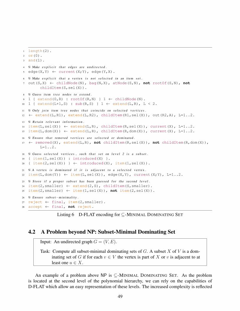
1 length(2).2 or(0).3 and(1).

4 % Make e x p l i c i t t h a t edges a r e u n d i r e c t e d .5 edge(X,Y) ← current(X;Y), edge(Y,X).

6 % Make e x p l i c i t t h a t a v e r t e x i s n o t s e l e c t e d i n an i t em s e t .7 out(S,X) ← childNode(N), bag(N,X), atNode(S,N), not rootOf(S,N), not

childItem(S,sel(X)).

8 % Guess i t em t r e e nodes t o e x t e n d .9 1 { extend(0,R) : rootOf(R,N) } 1 ← childNode(N).

10 1 { extend(L+1,S) : sub(R,S) } 1 ← extend(L,R), L < 2.

11 % Only j o i n i t em t r e e nodes t h a t c o i n c i d e on s e l e c t e d v e r t i c e s .12 ← extend(L,R1), extend(L,R2), childItem(R1,sel(X)), out(R2,A), L=1..2.

13 % R e t a i n r e l e v a n t i n f o r m a t i o n .14 item(L,sel(X)) ← extend(L,R), childItem(R,sel(X)), current(X), L=1..2.15 item(L,dom(X)) ← extend(L,R), childItem(R,dom(X)), current(X), L=1..2.

16 % Ensure t h a t removed v e r t i c e s a r e s e l e c t e d o r domina ted .17 ← removed(X), extend(L,R), not childItem(R,sel(X)), not childItem(R,dom(X)),

L=1..2.

18 % Guess s e l e c t e d v e r t i c e s , such t h a t s e t on l e v e l 2 i s a s u b s e t .19 { item(1,sel(X)) : introduced(X) }.20 { item(2,sel(X)) } ← introduced(X), item(1,sel(X)).

21 % A v e r t e x i s domina ted i f i t i s a d j a c e n t t o a s e l e c t e d v e r t e x .22 item(L,dom(Y)) ← item(L,sel(X)), edge(X,Y), current(X;Y), L=1..2.

23 % S t o r e i f a p r o p e r s u b s e t has been g u e s s e d f o r t h e second l e v e l .24 item(2,smaller) ← extend(2,S), childItem(S,smaller).25 item(2,smaller) ← item(1,sel(X)), not item(2,sel(X)).

26 % Ensure s u b s e t−m i n i m a l i t y .27 reject ← final, item(2,smaller).28 accept ← final, not reject.

Listing 6 D-FLAT encoding for ⊆-MINIMAL DOMINATING SET

4.2 A Problem beyond NP: Subset-Minimal Dominating Set

Input: An undirected graph G = (V,E).

Task: Compute all subset-minimal dominating sets of G. A subset X of V is a dom-inating set of G if for each v ∈ V the vertex is part of X or v is adjacent to atleast one u ∈ X .

An example of a problem above NP is ⊆-MINIMAL DOMINATING SET. As the problemis located at the second level of the polynomial hierarchy, we can rely on the capabilities ofD-FLAT which allow an easy representation of these levels. The increased complexity is reflected

49

in D-FLAT by the necessity of adding an additional level to the item trees. Listing 6 shows that thisis done by specifying the predicates length/2, and/1 and or/1. Via the predicate length/2,D-FLAT is instructed to create item tree branches of length 2. The facts or(0) and and(1) areused to inform D-FLAT that the problem instance is positive if there is an accepting node at depth1 such that all its children are accepting. Similar to other problems of the same complexity, also⊆-MINIMAL DOMINATING SET is tackled by guessing a solution candidate for the basic problemvariant on the first level. On the second level, for each subset of the selected vertices of level 1 ithas to hold that it is no dominating set unless the subset and the original selection coincide.

In the first lines of the encoding, we specify item tree branches of length 2, and we define thatthe first level is, notionally, existentially quantified, while the second one is universally quantified.This way we can capture problems in ΣP

2 . The use of item tree branches of length greater than 1requires slight modifications to the original encoding for the MINIMUM DOMINATING SET prob-lem. Syntactically, the arity of some predicates (among them are extend, item and auxItem)increases by one because we need to specify at which item tree branch level we want to store, e.g.,an item. Clearly, we also need additional code for checking the subset-minimality of a guess on thefirst level. As the tasks we want to compute at both levels are very similar, we could simply copymost of the rules from the encoding of MINIMUM DOMINATING SET and then adapt them. Here,the modeling language of Gringo comes into play and allows us to simply reuse almost all existingrules without the need for duplicated code. In this example, this is achieved by adding L=1..2 tothe relevant rules where a level specification is needed. The variable L is then instantiated to bothconstants 1 and 2 by the grounder, allowing us to capture both levels by writing only one rule.

In detail, the algorithm presented in Listing 6 works as follows. Similar to the encoding for theMINIMUM DOMINATING SET problem, we guess for each level which item tree node is extended,and via a constraint we ensure that the selected vertices coincide. Afterwards, we guess for eachintroduced vertex if it is selected at the first level and if this is the case, we guess if it is also selectedat the second level. This way, it is ensured that the selection on the second level is always a subsetof the selection on the first level and we derive the atom item(2,smaller) when it is a strictsubset. To remove all solution candidates that are not subset-minimal, we derive reject in thefinal node of the tree decomposition whenever there is evidence of a smaller dominating set. Allremaining candidates are then known to be indeed valid solutions and we derive accept for them.

As it turns out that DP algorithms for problems of the second level of the polynomial hierarchyoften follow recurring patterns as sketched above, there is also a “spin-off” of D-FLAT, calledD-FLAT2, that provides dedicated functionality for problems of this kind. As an example D-FLAT2

generates the DP algorithm for ⊆-MINIMAL DOMINATING SET directly from an encoding forthe standard DOMINATING SET problem. Describing this approach requires additional formalmachinery, and thus, we decided to not discuss D-FLAT2 in this report. The reader is referred to[13] for further reading.

4.3 Default Join in PracticeIn this section we will present the use of the --default-join option presented in Section 3.7.1,by comparing an encoding of the MINIMUM DOMINATING SET problem which uses default join,

50

1 % Make e x p l i c i t t h a t edges a r e u n d i r e c t e d .2 edge(X,Y) ← current(X;Y), edge(Y,X).

3 1 { extend(R) : childRow(R,N) } 1 ← childNode(N).

4 % R e t a i n r e l e v a n t i n f o r m a t i o n .5 item(sel(X)) ← extend(R), childItem(R,sel(X)), current(X).6 auxItem(dom(X)) ← extend(R), childAuxItem(R,dom(X)), current(X).

7 % Ensure t h a t removed v e r t i c e s a r e s e l e c t e d o r domina ted .8 ← removed(X), extend(R), not childItem(R,sel(X)), not childAuxItem(R,dom(X)).

9 % Guess s e l e c t e d v e r t i c e s .10 { item(sel(X)) : introduced(X) }.

11 % A v e r t e x i s domina ted i f i t i s a d j a c e n t t o a s e l e c t e d v e r t e x .12 auxItem(dom(Y)) ← item(sel(X)), edge(X,Y), current(X;Y).

13 % Leaf node c o s t s .14 cost(NC) ← NC = #count{ X : item(sel(X)) }, initial.15 % Exchange node c o s t s .16 cost(CC + NC) ← extend(R), childCost(R,CC),

NC = #count{ X : item(sel(X)), introduced(X) }, numChildNodes == 1.17 % C o s t s c o r r e s p o n d i n g on ly t o c u r r e n t node .18 currentCost(CC) ← CC = #count{ W,X : item(sel(X)), weight(X,W) }.

Listing 7 D-FLAT encoding for MINIMUM DOMINATING SET with default join

in Listing 7 to the one in Listing 4, which does not. Both are designed for weakly normalizedtree decompositions and, as we only need item trees of height 1, they use D-FLAT’s simplifiedinterface presented in Section 3.4.2. Using default join makes the rules in lines 4 and 7 from theencoding in Listing 4 superfluous, as the merge on specific items is done implicitly at join nodes.Nevertheless, we do need to specify on which types of items the merge should be done. As thefinal solutions must be consistent in the vertices belonging to the dominating sets, also the mergemust be done only on items of sel/1. This is why dom/1 is an auxiliary item in Listing 7. Further,instead of calculating the cost value in join nodes ourselves (line 22 in Listing 4), we just need tocalculate the current cost, as seen in line 18 in Listing 7.

4.4 Built-in Counters in PracticeNext, we will present the use of built-in D-FLAT counters in practice, based on encodings of vari-ants of the MINIMUM DOMINATING SET problem for weakly normalized tree decompositions, us-ing D-FLAT’s simplified interface presented in Section 3.4.2 and the option --default-joinpresented in Section 3.7.1. We will show how to use the output predicates counterInc/3+ andcurrentCounterInc/3+ by comparing an encoding of the MINIMUM WEIGHTED DOMINAT-ING SET problem which uses counter incrementation for calculating costs with one that does not.Further, we will illustrate the use of the output predicates counter/2 and currentCounter/2by comparing encodings of the GENERALIZED MINIMUM WEIGHTED DOMINATING SET prob-lem with and without built-in counters for every vertex to keep track of the number of dominating

51

1 % Make e x p l i c i t t h a t edges a r e u n d i r e c t e d .2 edge(X,Y) ← current(X;Y), edge(Y,X).

3 1 { extend(R) : childRow(R,N) } 1 ← childNode(N).

4 % R e t a i n r e l e v a n t i n f o r m a t i o n .5 item(sel(X)) ← extend(R), childItem(R,sel(X)), current(X).6 auxItem(dom(X)) ← extend(R), childAuxItem(R,dom(X)), current(X).

7 % Ensure t h a t removed v e r t i c e s a r e s e l e c t e d o r domina ted .8 ← removed(X), extend(R), not childItem(R,sel(X)), not childAuxItem(R,dom(X)).

9 % Guess s e l e c t e d v e r t i c e s .10 { item(sel(X)) : introduced(X) }.

11 % A v e r t e x i s domina ted i f i t i s a d j a c e n t t o a s e l e c t e d v e r t e x .12 auxItem(dom(Y)) ← item(sel(X)), edge(X,Y), current(X;Y).

13 % Leaf node c o s t s .14 cost(NC) ← NC = #sum{ W,X : item(sel(X)), weight(X,W) }, initial.15 % Exchange node c o s t s .16 cost(CC + NC) ← extend(R), childCost(R,CC),

NC = #sum{ W,X : item(sel(X)), introduced(X), weight(X,W) }.17 % C o s t s c o r r e s p o n d i n g on ly t o c u r r e n t node .18 currentCost(CC) ← CC = #sum{ W,X : item(sel(X)), weight(X,W) }.

Listing 8 D-FLAT encoding for MINIMUM WEIGHTED DOMINATING SET

vertices.We define the MINIMUM WEIGHTED DOMINATING SET problem as follows:

Input: An undirected graph G = (V,E) with weighted vertices.

Task: Compute all weight-minimal dominating sets of G. A subset X of V is a dom-inating set of G if for each v ∈ V the vertex is part of X or v is adjacent to atleast one u ∈ X .

In Listing 8 we see a possibility to encode the optimization variant of MINIMUM DOMINATING

SET in D-FLAT, where we minimize on the sum of vertex weights instead of the cardinality of thedominating set. As we only need item trees of height 1, we work again in table mode, and withdefault join, like in Listing 7. Compared to the latter, the encoding in Listing 8 uses a sum insteadof a count aggregate, as the costs represent the sum of the weights of the selected vertices.

In Listing 9 we replace lines 13–18 from Listing 8 in order to illustrate the technique of incre-menting counter values, in our case costs, instead of recalculating them in every ASP call. Therule in line 14 will be instantiated by the grounder as many times as many selected vertices thereare in the current partial solution candidate and D-FLAT will add each weight value to the cost ofthe latter. As we use the --default-join option we also increment the value of the currentcounter by the weights of newly introduced vertices (line 16) and decrement it by the weights ofthe removed vertices (line 18).

52

1 % Make e x p l i c i t t h a t edges a r e u n d i r e c t e d .2 edge(X,Y) ← current(X;Y), edge(Y,X).

3 1 { extend(R) : childRow(R,N) } 1 ← childNode(N).

4 % R e t a i n r e l e v a n t i n f o r m a t i o n .5 item(sel(X)) ← extend(R), childItem(R,sel(X)), current(X).6 auxItem(dom(X)) ← extend(R), childAuxItem(R,dom(X)), current(X).

7 % Ensure t h a t removed v e r t i c e s a r e s e l e c t e d o r domina ted .8 ← removed(X), extend(R), not childItem(R,sel(X)), not childAuxItem(R,dom(X)).

9 % Guess s e l e c t e d v e r t i c e s .10 { item(sel(X)) : introduced(X) }.

11 % A v e r t e x i s domina ted i f i t i s a d j a c e n t t o a s e l e c t e d v e r t e x .12 auxItem(dom(Y)) ← item(sel(X)), edge(X,Y), current(X;Y).

13 % I n c r e m e n t t h e c o s t by t h e w e i g h t s o f newly i n t r o d u c e d v e r t i c e s .14 counterInc(cost,W,X) ← introduced(X), item(sel(X)), weight(X,W).15 % I n c r e m e n t t h e c u r r e n t c o s t by t h e w e i g h t s o f newly i n t r o d u c e d v e r t i c e s .16 currentCounterInc(cost,W,X) ← introduced(X), item(sel(X)), weight(X,W).17 % Decrement t h e c u r r e n t c o s t by t h e w e i g h t s o f newly removed v e r t i c e s .18 currentCounterInc(cost,-W,X) ← removed(X), extend(R), childItem(R,sel(X)),

weight(W,X).

Listing 9 D-FLAT encoding for MINIMUM WEIGHTED DOMINATING SET using counterincrementation for cost calculation

Next, we will show how to use counters based on the GENERALIZED MINIMUM WEIGHTED

PERFECT DOMINATING SET problem, which we define as follows:

Input: An undirected graph G = (V,E) with weighted vertices and upper and/orlower bounds defining for a vertex by how many other vertices it may be domi-nated.

Task: Compute all weight-minimal dominating sets ofG such that the defined boundsare respected. A subset X of V is a dominating set of G if for each v ∈ V thevertex is part of X or v is adjacent to at least one u ∈ X (i.e. is dominated byat least one u ∈ X).

Listing 10 shows the D-FLAT encoding for the GENERALIZED MINIMUM WEIGHTED PER-FECT DOMINATING SET problem, which implements the changes needed for the vertices to re-spect the given bounds, as compared to the encoding in Listing 8. Instead of using an auxiliaryitem dom/1, which tells that the vertex given as its only argument is dominated, we need one thattakes also the number of vertices our vertex is dominated by and the name of the current nodeas arguments and in fact tells for each vertex by how many vertices it is dominated (in case it isnot dominated, the value of the second argument is 0). Storing the name of the current node isnecessary as we need a supplementary node above each join node bearing an identical bag (option--post-join). There we can adjust the values of dom/3 items, as the default join just passes

53

1 % Make e x p l i c i t t h a t edges a r e u n d i r e c t e d .2 edge(X,Y) ← current(X;Y), edge(Y,X).

3 1 { extend(R) : childRow(R,N) } 1 ← childNode(N).

4 % R e t a i n which v e r t i c e s have a l r e a d y been s e l e c t e d .5 item(sel(X)) ← extend(R), childItem(R,sel(X)), current(X).

6 % Ensure t h a t removed v e r t i c e s a r e s e l e c t e d and r e s p e c t d o m i n a t i o n bounds .7 ← removed(X), extend(R), not childItem(R,sel(X)),

childAuxItem(R,dom(X,N,CR)), lowerBound(X,B), N<B.8 ← removed(X), extend(R), not childItem(R,sel(X)),

childAuxItem(R,dom(X,N,CR)), upperBound(X,B), N>B.

9 % Guess s e l e c t e d v e r t i c e s .10 { item(sel(X)) : introduced(X) }.

11 % Deduct f o r each v e r t e x by how many o t h e r v e r t i c e s i t i s domina ted .12 auxItem(dom(Y,N,CR)) ← extend(R), currentNode(CR), introduced(Y),

not item(sel(Y)), 1 #count { CH: childAuxItem(R,n(CH)) } 1,N = #count { X : item(sel(X)), edge(X,Y) }.

13 auxItem(dom(Y,N1+N0,CR)) ← extend(R), currentNode(CR), current(Y),1 #count { CH: childAuxItem(R,n(CH)) } 1, childAuxItem(R,dom(Y,N1,CH1)),N0 = #count { X : item(sel(X)), edge(X,Y), introduced(X) }.

14 auxItem(dom(Y,N1+N2-N12,CR)) ← extend(R), currentNode(CR), current(Y),childAuxItem(R,dom(Y,N1,CH1)), childAuxItem(R,dom(Y,N2,CH2)), CH1 6= CH2,N12 = #count { X : item(sel(X)), edge(X,Y) }.

15 auxItem(n(CR)) ← currentNode(CR).

16 % Leaf node c o s t s .17 cost(NC) ← NC = #sum{ W,X : item(sel(X)), weight(X,W) }, initial.18 % Exchange node c o s t s .19 cost(CC + NC) ← extend(R), childCost(R,CC),

NC = #sum{ W,X : item(sel(X)), introduced(X), weight(X,W) }.20 % C o s t s c o r r e s p o n d i n g on ly t o c u r r e n t node .21 currentCost(CC) ← CC = #sum { W,X : item(sel(X)), weight(X,W) }.

Listing 10 D-FLAT encoding for GENERALIZED MINIMUM WEIGHTED PERFECT

DOMINATING SET

auxiliary items through without merging them and we need to do this explicitly. In line 12 we countfor each vertex which is newly introduced into an exchange node, by how many other vertices itis dominated, in line 13 we calculate the latter value for vertices which are not newly introducedby adding the number of dominating vertices in the child node to the number of newly introduceddominating vertices and in line 14 we merge the values coming from different branches below thejoin node, by the inclusion-exclusion principle. In line 15 we define the n/1 predicate which isnecessary when checking that we are not dealing with a post-processing node. Further, instead ofline 8 from Listing 8, we now have two constraint rules in lines 7–8 which also check for eachvertex the lower and upper bound of dominating vertices, respectively.

Listing 11 illustrates how such an encoding can be simplified by means of counters. Instead ofdom/3 auxiliary items we now use counters which implicitly keep track of these values and let the

54

1 % Make e x p l i c i t t h a t edges a r e u n d i r e c t e d .2 edge(X,Y) ← current(X;Y), edge(Y,X).

3 1 { extend(R) : childRow(R,N) } 1 ← childNode(N).

4 % R e t a i n which v e r t i c e s have a l r e a d y been s e l e c t e d .5 item(sel(X)) ← extend(R), childItem(R,sel(X)), current(X).

6 % Ensure t h a t removed v e r t i c e s a r e s e l e c t e d and r e s p e c t d o m i n a t i o n bounds .7 ← removed(X), extend(R), not childItem(R,sel(X)), childCounter(R,X,N),

lowerBound(X,B), N<B.8 ← removed(X), extend(R), not childItem(R,sel(X)), childCounter(R,X,N),

upperBound(X,B), N>B.

9 % Guess s e l e c t e d v e r t i c e s .10 { item(sel(X)) : introduced(X) }.

11 % Keep t r a c k f o r each v e r t e x by how many o t h e r v e r t i c e s i t i s dominated , u s i n g c o u n t e r s .12 counter(Y,N) ← introduced(Y), not item(sel(Y)),

N = #count { X : item(sel(X)), edge(X,Y) }.13 counter(Y,N0+N1) ← extend(R), current(Y), childCounter(R,Y,N1),

N0 = #count { X : item(sel(X)), edge(X,Y), introduced(X) }.14 currentCounter(Y,N) ← current(Y), not item(sel(Y)),

N = #count { X: item(sel(X)), edge(X,Y) }.15 counterRem(Y) ← removed(Y).

16 % Leaf node c o s t s .17 cost(NC) ← NC = #sum{ W,X : item(sel(X)), weight(X,W) }, initial.18 % Exchange node c o s t s .19 cost(CC + NC) ← extend(R), childCost(R,CC),

NC = #sum{ W,X : item(sel(X)), introduced(X), weight(X,W) }.20 % C o s t s c o r r e s p o n d i n g on ly t o c u r r e n t node .21 currentCost(CC) ← CC = #sum { W,X : item(sel(X)), weight(X,W) }.

Listing 11 D-FLAT encoding for GENERALIZED MINIMUM WEIGHTED PERFECT

DOMINATING SET with counters

default join do the merge such that a post-processing node is not necessary anymore. Lines 12–13have the same role as before, yet they are simpler because there is no need to check whether weare in a post-processing node and we can make use of the input predicate childCounter/3. Next,instead of having to explicitly merge values in the post-processing node, we just need to keep trackof the value of the counter corresponding to the current tree decomposition node, which is donein line 14. In order to not carry around unnecessary counters in the system, in line 15 we removea counter if the corresponding vertex has been removed from the tree decomposition. Further, inlines 7–8 we can now also use childCounter/3, instead of childAuxItem/2.

4.5 Lazy Evaluation in PracticeIn order to illustrate how to employ D-FLAT with lazy evaluation, we adapted the D-FLAT encod-ing from Listing 8 of the previously defined MINIMUM WEIGHTED DOMINATING SET problem

55

1 % Make e x p l i c i t t h a t edges a r e u n d i r e c t e d .2 edge(X,Y) ← current(X;Y), edge(Y,X).

3 % D e c l a r e atoms p a s s i n g on i n f o r m a t i o n from c h i l d rows .4 #external childItem(sel(X)) : childNode(N), bag(N,X).5 #external childAuxItem(dom(X)) : childNode(N), bag(N,X).6 #external childCost(0..N) : maxSumOfWeights(N).

7 % R e t a i n r e l e v a n t i n f o r m a t i o n .8 item(sel(X)) ← childItem(sel(X)), current(X).9 auxItem(dom(X)) ← childAuxItem(dom(X)), current(X).

10 % Ensure t h a t removed v e r t i c e s a r e s e l e c t e d o r domina ted .11 ← removed(X), not childItem(sel(X)), not childAuxItem(dom(X)).

12 % Guess s e l e c t e d v e r t i c e s .13 { item(sel(X)) : introduced(X) }.

14 % A v e r t e x i s domina ted i f i t i s a d j a c e n t t o a s e l e c t e d v e r t e x .15 auxItem(dom(Y)) ← item(sel(X)), edge(X,Y), current(X;Y).

16 % Leaf node c o s t s .17 cost(NC) ← NC = #sum{ W,X : item(sel(X)), weight(X,W) }, initial.18 % Exchange node c o s t s .19 cost(CC + NC) ← childCost(CC),

NC = #sum{ W,X : item(sel(X)), introduced(X), weight(X,W) }.20 % C o s t s c o r r e s p o n d i n g on ly t o c u r r e n t node .21 currentCost(CC) ← CC = #sum { W,X : item(sel(X)), weight(X,W) }.

Listing 12 D-FLAT encoding for solving MINIMUM WEIGHTED DOMINATING SET with lazyevaluation

for this purpose, resulting in Listing 12, which also makes use of the --default-join option.Compared to the former encoding, the one for lazy evaluation does not need the rule in line 3 any-more since grounding is done as an initial step at each table without information about any childrow and the truth values of the atoms that depend on child rows are successively set to those cor-responding to the child row currently considered. Instead, we need lines 4–5 so the grounder willnot assume an atom childItem(sel(X)) or childAuxItem(dom(X)) to be false, where X isa vertex in the bag of the child node. Furthermore, in line 6, we declare which are the possible val-ues for childCost/1. For this, we expect that the input contains a fact maxSumOfWeights(W),where W is the maximum cost that a partial solution may have. Everything else stays the same asin Listing 8, except for the fact that there is no reference to any child table row and the extend/1predicate is not used anymore.

56

5 ConclusionIn this report we presented the D-FLAT system (as of version 1.2.5) for developing algorithms thatemploy dynamic programming on tree decompositions. The key feature of D-FLAT is that it letsthe user specify such algorithms in the declarative language of ASP. This makes it well suited forrapid prototyping.

After presenting the background on ASP and tree decompositions, we explained the differentcomponents of D-FLAT in detail, as well as the interface that is used for communication be-tween the system and the problem-specific encodings. We discussed new features that have beenadded over time, such as built-in counters and lazy evaluation, and we presented the improvementsbrought by using the htd framework. Then we showed how D-FLAT can be applied to a selectionof problems to underline the usability of our approach.

The fact that we have been able to come up with relatively simple D-FLAT encodings forvarious different problems shows that our system is indeed well suited for rapid prototyping ofdecomposition-based algorithms. Even more, D-FLAT can be a competitive solver in certain set-tings, in particular if the treewidth of the instances to be solved is small. The proposed ASPinterface is general enough to accommodate quite different kinds of problems.

There are a number of related works that concern ASP and tree decomposition techniques,some of which originate from the experience we gained in developing D-FLAT. DYNASP [34, 35]is a new ASP solver for ground answer-set programs that employs dynamic programming on treedecompositions. Such a system can be beneficial if the (incidence graph of a) ground programhas rather small treewidth. As has been shown recently, for certain classes of ASP encodings thetreewidth of the grounded program remains small given that the instance also has small treewidth[15]. Finally, we would like to mention the lpopt tool [11] that aims at decomposing non-groundrules.

57

References[1] Michael Abseher, Bernhard Bliem, Gunther Charwat, Frederico Dusberger, Markus Hecher,

and Stefan Woltran. D-FLAT: Progress report. Technical Report DBAI-TR-2014-86, DBAI,Vienna University of Technology, 2014.

[2] Michael Abseher, Marius Moldovan, and Stefan Woltran. Providing built-in counters in adeclarative dynamic programming environment. In Proc. KI, volume 9904 of LNCS, pages3–16. Springer, 2016.

[3] Michael Abseher, Nysret Musliu, and Stefan Woltran. htd–a free, open-source frameworkfor tree decompositions and beyond. Technical Report DBAI-TR-2014-96, DBAI, ViennaUniversity of Technology, 2016.

[4] Michael Abseher, Nysret Musliu, and Stefan Woltran. htd - A Free, Open-Source Frameworkfor (Customized) Tree Decompositions and Beyond. In Proc. CPAIOR, volume 10335 ofLNCS, pages 376–386. Springer, 2017.

[5] Michael Abseher, Nysret Musliu, and Stefan Woltran. Improving the efficiency of dynamicprogramming on tree decompositions via machine learning. Journal of Artificial IntelligenceResearch, 58:829–858, 2017.

[6] Rachit Agarwal, Philip Brighten Godfrey, and Sariel Har-Peled. Approximate distancequeries and compact routing in sparse graphs. In Proc. INFOCOM, pages 1754–1762. IEEE,2011.

[7] Mario Alviano, Francesco Calimeri, Wolfgang Faber, Giovambattista Ianni, and NicolaLeone. Function symbols in ASP: Overview and perspectives. In NMR – Essays CelebratingIts 30th Anniversary, pages 1–24. College Publications, London, 2011.

[8] Stefan Arnborg, Derek G. Corneil, and Andrzej Proskurowski. Complexity of finding em-beddings in a k-tree. SIAM J. Algebraic Discrete Methods, 8(2):277–284, 1987.

[9] Markus Aschinger, Conrad Drescher, Georg Gottlob, Peter Jeavons, and EvgenijThorstensen. Structural decomposition methods and what they are good for. In Proc. STACS,volume 9 of LIPICS, pages 12–28. Schloss Dagstuhl – Leibniz-Zentrum fur Informatik, 2011.

[10] Chitta Baral. Knowledge Representation, Reasoning and Declarative Problem Solving. Cam-bridge University Press, 2003.

[11] Manuel Bichler, Michael Morak, and Stefan Woltran. lpopt: A rule optimization tool for an-swer set programming. In Proc. LOPSTR, volume 10184 of LNCS, pages 114–130. Springer,2017.

[12] Bernhard Bliem. Decompose, Guess & Check: Declarative problem solving on tree decom-positions. Master’s thesis, Vienna University of Technology, 2012.

58

[13] Bernhard Bliem, Gunther Charwat, Markus Hecher, and Stefan Woltran. D-FLATˆ2: Subsetminimization in dynamic programming on tree decompositions made easy. FundamentaInformaticae, 147(1):27–61, 2016.

[14] Bernhard Bliem, Benjamin Kaufmann, Torsten Schaub, and Stefan Woltran. ASP for anytimedynamic programming on tree decompositions. In Proc. IJCAI, pages 979–986. IJCAI/AAAIPress, 2016.

[15] Bernhard Bliem, Marius Moldovan, Michael Morak, and Stefan Woltran. The impact oftreewidth on ASP grounding and solving. In Proc. IJCAI, pages 852–858. ijcai.org, 2017.

[16] Bernhard Bliem, Reinhard Pichler, and Stefan Woltran. Declarative dynamic programmingas an alternative realization of Courcelle’s theorem. In Proc. IPEC, volume 8246 of LNCS,pages 28–40. Springer, 2013.

[17] Bernhard Bliem, Reinhard Pichler, and Stefan Woltran. Implementing Courcelle’s Theoremin a declarative framework for dynamic programming. Journal of Logic and Computation,2017. Early access available (DOI 10.1093/logcom/exv089), to appear.

[18] Hans L. Bodlaender. A tourist guide through treewidth. Acta Cybern., 11(1-2):1–22, 1993.

[19] Hans L. Bodlaender. A linear-time algorithm for finding tree-decompositions of smalltreewidth. SIAM J. Comput., 25(6):1305–1317, 1996.

[20] Hans L. Bodlaender. Discovering treewidth. In Proc. SOFSEM, volume 3381 of LNCS, pages1–16. Springer, 2005.

[21] Hans L. Bodlaender and Arie M. C. A. Koster. Combinatorial optimization on graphs ofbounded treewidth. Comput. J., 51(3):255–269, 2008.

[22] Hans L. Bodlaender and Arie M. C. A. Koster. Treewidth computations I. Upper bounds. Inf.Comput., 208(3):259–275, 2010.

[23] Gerhard Brewka, Thomas Eiter, and Mirosław Truszczynski. Answer set programming at aglance. Commun. ACM, 54(12):92–103, 2011.

[24] Francesco Calimeri, Susanna Cozza, Giovambattista Ianni, and Nicola Leone. Computablefunctions in ASP: Theory and implementation. In Proc. ICLP, volume 5366 of LNCS, pages407–424. Springer, 2008.

[25] Ashok K. Chandra, Dexter Kozen, and Larry J. Stockmeyer. Alternation. J. ACM, 28(1):114–133, 1981.

[26] Keith L. Clark. Negation as failure. In Logic and Data Bases, pages 293–322. Springer,1977.

59

[27] Bruno Courcelle. The monadic second-order logic of graphs. I. Recognizable sets of finitegraphs. Inf. Comput., 85(1):12–75, 1990.

[28] Evgeny Dantsin, Thomas Eiter, Georg Gottlob, and Andrei Voronkov. Complexity and ex-pressive power of logic programming. ACM Comput. Surv., 33(3):374–425, 2001.

[29] Rina Dechter. Bucket elimination: A unifying framework for reasoning. Artif. Intell., 113(1–2):41–85, 1999.

[30] Holger Dell, Thore Husfeldt, Bart M. P. Jansen, Petteri Kaski, Christian Komusiewicz, andFrances A. Rosamond. The first parameterized algorithms and computational experimentschallenge. In Proc. IPEC, volume 63 of LIPIcs, pages 30:1–30:9. Schloss Dagstuhl - Leibniz-Zentrum fuer Informatik, 2017.

[31] Artan Dermaku, Tobias Ganzow, Georg Gottlob, Benjamin J. McMahan, Nysret Musliu, andMarko Samer. Heuristic methods for hypertree decomposition. In Proc. MICAI, volume 5317of LNCS, pages 1–11. Springer, 2008.

[32] Thomas Eiter and Georg Gottlob. On the computational cost of disjunctive logic program-ming: Propositional case. Ann. Math. Artif. Intell., 15(3-4):289–323, 1995.

[33] Thomas Eiter, Georg Gottlob, and Heikki Mannila. Disjunctive Datalog. ACM Trans.Database Syst., 22(3):364–418, 1997.

[34] Johannes Klaus Fichte, Markus Hecher, Michael Morak, and Stefan Woltran. Answer setsolving with bounded treewidth revisited. In Proc. LPNMR, volume 10377 of LNCS, pages132–145. Springer, 2017.

[35] Johannes Klaus Fichte, Markus Hecher, Michael Morak, and Stefan Woltran. Dynasp2.5:Dynamic programming on tree decompositions in action. CoRR, abs/1706.09370, 2017.

[36] Martin Gebser, Roland Kaminski, Benjamin Kaufmann, Marius Lindauer, Max Ostrowski,Javier Romero, Torsten Schaub, and Sven Thiele. A user’s guide to gringo, clasp, clingo, andiclingo. Second Edition. Available at http://potassco.sourceforge.net, 2015.

[37] Martin Gebser, Roland Kaminski, Max Ostrowski, Torsten Schaub, and Sven Thiele. On theinput language of ASP grounder gringo. In Proc. LPNMR, volume 5753 of LNCS, pages502–508. Springer, 2009.

[38] Martin Gebser, Benjamin Kaufmann, Roland Kaminski, Max Ostrowski, Torsten Schaub,and Marius Thomas Schneider. Potassco: The Potsdam answer set solving collection. AICommun., 24(2):107–124, 2011.

[39] Michael Gelfond and Nicola Leone. Logic programming and knowledge representation –The A-Prolog perspective. Artif. Intell., 138(1-2):3–38, 2002.

60

[40] Michael Gelfond and Vladimir Lifschitz. The stable model semantics for logic programming.In Proc. ICLP/SLP, pages 1070–1080. The MIT Press, 1988.

[41] Michael Gelfond and Vladimir Lifschitz. Classical negation in logic programs and disjunctivedatabases. New Generation Comput., 9(3/4):365–386, 1991.

[42] Georg Gottlob, Nicola Leone, and Francesco Scarcello. Hypertree decompositions andtractable queries. J. Comput. Syst. Sci., 64(3):579–627, 2002.

[43] Jens Gramm, Arfst Nickelsen, and Till Tantau. Fixed-parameter algorithms in phylogenetics.Comput. J., 51(1):79–101, 2008.

[44] Xiuzhen Huang and Jing Lai. Parameterized graph problems in computational biology. InProc. IMSCCS, pages 129–132. IEEE, 2007.

[45] Matthieu Latapy and Clemence Magnien. Measuring fundamental properties of real-worldcomplex networks. CoRR, abs/cs/0609115, 2006.

[46] Nicola Leone, Gerald Pfeifer, Wolfgang Faber, Thomas Eiter, Georg Gottlob, Simona Perri,and Francesco Scarcello. The DLV system for knowledge representation and reasoning. ACMTrans. Comput. Log., 7(3):499–562, 2006.

[47] Vladimir Lifschitz. What is answer set programming? In Proc. AAAI, pages 1594–1597.AAAI Press, 2008.

[48] Victor W. Marek and Jeffrey B. Remmel. On the expressibility of stable logic programming.TPLP, 3(4-5):551–567, 2003.

[49] Victor W. Marek and Mirosław Truszczynski. Autoepistemic logic. J. ACM, 38(3):588–619,1991.

[50] Victor W. Marek and Mirosław Truszczynski. Stable models and an alternative logic pro-gramming paradigm. In The Logic Programming Paradigm: A 25-Year Perspective, pages375–398. Springer, 1999.

[51] Guy Melancon. Just how dense are dense graphs in the real world? A methodological note.In Proc. BELIV, pages 1–7. ACM Press, 2006.

[52] Rolf Niedermeier. Invitation to Fixed-Parameter Algorithms. Oxford Lecture Series in Math-ematics And Its Applications. Oxford University Press, 2006.

[53] Ilkka Niemela. Logic programs with stable model semantics as a constraint programmingparadigm. Ann. Math. Artif. Intell., 25(3-4):241–273, 1999.

[54] Neil Robertson and Paul D. Seymour. Graph minors. III. Planar tree-width. J. Comb. Theory,Ser. B, 36(1):49–64, 1984.

61

[55] John S. Schlipf. The expressive powers of the logic programming semantics. J. Comput. Syst.Sci., 51(1):64–86, 1995.

[56] Mikkel Thorup. All structured programs have small tree-width and good register allocation.Inf. Comput., 142(2):159–181, 1998.

[57] Atsuko Yamaguchi, Kiyoko F. Aoki, and Hiroshi Mamitsuka. Graph complexity of chemicalcompounds in biological pathways. Genome Inform., 14:376–377, 2003.

62