technical appendix to the economics of density: evidence
TRANSCRIPT

Technical Appendix to The Economics of Density:Evidence from the Berlin Wall
Gabriel M. AhlfeldtLondon School of Economics
Stephen J. ReddingPrinceton University, NBER and CEPR
Daniel M. SturmLondon School of Economics and CEPR
Nikolaus WolfHumboldt University and CEPR
July 25, 2014
Contents
A.1 Introduction . . . . . . . . . . . . . . . . . . . . . . . . . . . . . . . . . . . . . . . . . . . . . 2A.2 Theoretical Model . . . . . . . . . . . . . . . . . . . . . . . . . . . . . . . . . . . . . . . . . 3
A.2.1 Preferences . . . . . . . . . . . . . . . . . . . . . . . . . . . . . . . . . . . . . . . . 4A.2.2 Distribution of Utility . . . . . . . . . . . . . . . . . . . . . . . . . . . . . . . . . . . 5A.2.3 Residence and Workplace Choices . . . . . . . . . . . . . . . . . . . . . . . . . . . . 6A.2.4 Production . . . . . . . . . . . . . . . . . . . . . . . . . . . . . . . . . . . . . . . . . 9A.2.5 Land Market Clearing . . . . . . . . . . . . . . . . . . . . . . . . . . . . . . . . . . 10A.2.6 Properties of General Equilibrium with Exogenous Location
Characteristics . . . . . . . . . . . . . . . . . . . . . . . . . . . . . . . . . . . . . . 11A.2.7 Properties of General Equilibrium with Agglomeration Forces . . . . . . . . . . . . 18
A.3 Calibration . . . . . . . . . . . . . . . . . . . . . . . . . . . . . . . . . . . . . . . . . . . . . 21A.3.1 Determining A, B, ϕ from α, β, µ, ε, κ and the Observed Data . . . . . . . . . 22
A.3.1.1 Wages . . . . . . . . . . . . . . . . . . . . . . . . . . . . . . . . . . . . . 22A.3.1.2 Adjusted Residential Amenities . . . . . . . . . . . . . . . . . . . . . . . 25A.3.1.3 Final Goods Productivity . . . . . . . . . . . . . . . . . . . . . . . . . . . 26A.3.1.4 Land Market Clearing . . . . . . . . . . . . . . . . . . . . . . . . . . . . . 26A.3.1.5 Utility, Amenities and Productivity . . . . . . . . . . . . . . . . . . . . . 28A.3.1.6 One-to-One Mapping from α, β, µ, ε, κ and the Observed Data to A,
B, ϕ . . . . . . . . . . . . . . . . . . . . . . . . . . . . . . . . . . . . . . 28A.3.2 Determining a, b from α, β, µ, ε, κ, λ, δ, η, ρ and the Observed Data . . . . . . 29
A.4 Structural Estimation . . . . . . . . . . . . . . . . . . . . . . . . . . . . . . . . . . . . . . . . 31
1

A.4.1 Structural Residuals . . . . . . . . . . . . . . . . . . . . . . . . . . . . . . . . . . . . 32A.4.2 Moment Conditions . . . . . . . . . . . . . . . . . . . . . . . . . . . . . . . . . . . . 33A.4.3 GMM Estimation . . . . . . . . . . . . . . . . . . . . . . . . . . . . . . . . . . . . . 35A.4.4 Estimation Algorithms . . . . . . . . . . . . . . . . . . . . . . . . . . . . . . . . . . 36A.4.5 Identication . . . . . . . . . . . . . . . . . . . . . . . . . . . . . . . . . . . . . . . 38
A.5 Counterfactuals . . . . . . . . . . . . . . . . . . . . . . . . . . . . . . . . . . . . . . . . . . . 41A.6 Monte Carlo . . . . . . . . . . . . . . . . . . . . . . . . . . . . . . . . . . . . . . . . . . . . . 43A.7 Introducing Non-traded Goods . . . . . . . . . . . . . . . . . . . . . . . . . . . . . . . . . . 45
A.7.1 Non-Traded Goods by Workplace . . . . . . . . . . . . . . . . . . . . . . . . . . . . 46A.7.2 Non-Traded Goods by Residence . . . . . . . . . . . . . . . . . . . . . . . . . . . . 47
A.8 Additional Reduced-Form Empirical Results . . . . . . . . . . . . . . . . . . . . . . . . . . . 47A.8.1 Maps of Changes in Floor Prices . . . . . . . . . . . . . . . . . . . . . . . . . . . . . 47A.8.2 Baseline Dierence-in-Dierence Specication . . . . . . . . . . . . . . . . . . . . 48A.8.3 Further Reduced-Form Evidence . . . . . . . . . . . . . . . . . . . . . . . . . . . . . 48
A.9 Additional Structural Estimates . . . . . . . . . . . . . . . . . . . . . . . . . . . . . . . . . . 50A.9.1 Gravity, Productivity and Amenities . . . . . . . . . . . . . . . . . . . . . . . . . . 50A.9.2 Structural Estimation . . . . . . . . . . . . . . . . . . . . . . . . . . . . . . . . . . . 50
A.10 Data Sources and Denitions . . . . . . . . . . . . . . . . . . . . . . . . . . . . . . . . . . . 50A.10.1 Employment at Place of Residence 1930s . . . . . . . . . . . . . . . . . . . . . . . . 51A.10.2 Employment at workplace . . . . . . . . . . . . . . . . . . . . . . . . . . . . . . . . 51A.10.3 Travel Times Between Blocks in Berlin . . . . . . . . . . . . . . . . . . . . . . . . . 52A.10.4 Block Characteristics . . . . . . . . . . . . . . . . . . . . . . . . . . . . . . . . . . . 54A.10.5 Commuting Survey Data . . . . . . . . . . . . . . . . . . . . . . . . . . . . . . . . . 55A.10.6 Micro Data on Land Transactions . . . . . . . . . . . . . . . . . . . . . . . . . . . . 56
A.1 Introduction
This technical appendix contains additional supplementary material for the paper. Section A.2 presentsa more detailed analysis of the theoretical model. We report the technical derivations of the expressionsreported in the paper. We also establish a number of results about the properties of the general equilibriumwith exogenous location characteristics and endogenous agglomeration forces.
Section A.3 calibrates the model for known parameter values and shows that there is a one-to-one map-ping from these known parameters and the observed data to unobserved location characteristics. Thereforethese unobserved location characteristics correspond to structural residuals that are functions of the pa-rameters and the observed data.
Section A.4 turns to the structural estimation of the model, where both the parameters and unobservedlocation characteristics are unknown and to be estimated. We derive the moment conditions used in theestimation and review the Generalized Method of Moments (GMM) estimator as applied to our setting. We
2

discuss the computational algorithms used to estimate the model and report the results of a grid search overthe parameter space that we use to characterize the properties of the GMM objective function.
Section A.5 uses the model to undertake counterfactuals for the eects of division and reunication.Section A.6 reports the results of a Monte Carlo exercise, in which we show that our estimation procedurecorrectly recovers the model parameters when the data are generated according to the model.
Section A.7 discusses an extension of the theoretical model to incorporate non-traded goods. SectionA.8 presents additional reduced-form empirical results discussed in the paper. Section A.9 reports additionalstructural estimation results discussed in the paper. Section A.10 contains further information about thedata sources and denitions.
A.2 Theoretical Model
In this section, we develop in further detail the theoretical model outlined in the paper. We present thecomplete technical derivations for all the expressions and results reported in the paper. In the interests ofclarity and to ensure that this section of the web appendix is self-contained, we reproduce some materialfrom the paper, but also include the intermediate steps for the derivation of expressions.
We consider a city embedded within a wider economy. The city consists of a set of discrete locations orblocks, which are indexed by i = 1, ..., S. The city is populated by an endogenous measure of H workers,who are perfectly mobile within the city and the larger economy. Each block has an eective supply of oorspace Li. Floor space can be used commercially or residentially, and we denote the endogenous fractionsof oor space allocated to commercial and residential use by θi and (1− θi), respectively.
Workers decide whether or not to move to the city before observing idiosyncratic utility shocks for eachpossible pair of residence and employment locations within the city. If a worker decides to move to the city,they observe these realizations for idiosyncratic utility, and pick the pair of residence and employmentlocations within the city that maximizes their utility. Population mobility between the city and the widereconomy implies that the expected utility from moving to the city equals the reservation level of utility inthe wider economy U . Firms produce a single nal good, which is costlessly traded within the city andlarger economy, and is chosen as the numeraire (p = 1). 1
Locations dier in terms of their nal goods productivity (Ai), residential amenities (Bi), supply of oorspace (Li) and access to the transport network (τij). We rst develop the model with exogenous values ofthese location characteristics, before endogenizing them below.
1We follow the canonical urban model in assuming a single tradable nal good and examine the ability of this canonical modelto account quantitatively for the observed impact of division and reunication. In Section A.7 of this web appendix, we discussan extension of the model to introduce a non-traded good.
3

A.2.1 Preferences
Workers are risk neutral such that the utility of worker ω residing in block i and working in block j is linearin an aggregate consumption index (Cijω):2
Uijω = Cijω.
This aggregate consumption index depends on consumption of the single nal good (cijω), consumptionof residential oor space (`ijω), and three other components. First, residential amenities (Bi) that capturecommon characteristics that make a block a more or less attractive place to live (e.g. leafy streets and scenicviews). Second, the disutility from commuting from residence block i to workplace block j (dij ≥ 1). Third,there is an idiosyncratic shock that is specic to individual workers and varies with the worker’s blocks ofemployment and residence (zijω). This idiosyncratic shock captures the idea that individual workers canhave idiosyncratic reasons for living and working in dierent parts of the city. In particular, the aggregateconsumption index is assumed to take the Cobb-Douglas form:3
Cijω =Bizijωdij
(cijωβ
)β (`ijω
1− β
)1−β
, 0 < β < 1, (1)
where the iceberg commuting cost dij = eκτij ∈ [1,∞) increases with the travel time between blocksi and j (τij). Travel time is measured in minutes and is computed based on the transport network, asdiscussed further in the data section of this web appendix (Section A.10). The parameter κ controls thesize of commuting costs. Although we model commuting costs in terms of utility, there is an isomorphicformulation in terms of a reduction in eective units of labor, because the iceberg commuting cost dij = eκτij
enters the indirect utility function (5) below multiplicatively. As a result, commuting costs are proportionalto wages, and hence this specication captures changes over time in the opportunity cost of travel time.
We model the heterogeneity in the utility that workers derive from living and working in dierent partsof the city following McFadden (1974) and Eaton and Kortum (2002). For each worker ω living in block i andcommuting to block j, the idiosyncratic component of utility (zijω) is drawn from an independent Fréchetdistribution:
F (zijω) = e−TiEjz−εijω , Ti, Ej > 0, ε > 1, (2)
where the scale parameter Ti > 0 determines the average utility derived from living in block i, the scaleparameterEj > 0 determines the average utility derived from working in block j; and the shape parameterε > 1 controls the dispersion of idiosyncratic utility.
After observing her realizations for idiosyncratic utility for each pair of residence and employmentlocations, each worker chooses her blocks of residence and employment to maximize her utility, takingas given residential amenities, goods prices, factor prices, and the location decisions of other workers and
2To simplify the exposition, throughout the appendix, we index a worker’s block of residence by i or r and her block ofemployment by j or s unless otherwise indicated.
3For empirical evidence using US data in support of the constant housing expenditure share implied by the Cobb-Douglasfunctional form, see Davis and Ortalo-Magné (2011). The role played by residential amenities in inuencing utility is emphasizedin the literature following Roback (1982). See Albouy (2008) for a recent prominent contribution.
4

rms. Each worker is endowed with one unit of labor that is supplied inelastically with zero disutility.Combining our choice of the nal good as numeraire (pi = p = 1 for all i) with the rst-order conditionsfor consumer equilibrium, we obtain the following demands for the nal good and residential land forworker ω residing in block i and working in block j:
cijω = βwj, (3)
`ijω = (1− β)wjQi
, (4)
where wj is the wage received by the worker at her block of employment j (recall that commuting costsare incurred in terms of utility); Qi is the price of residential land at her block of residence i. We make thestandard assumption that income from land is accrued by absentee landlords and not spent within the city,although it is also possible to consider the case where it is redistributed lump sum to workers. Substitutingequilibrium consumption of the nal good (3) and residential land use (4) into utility (1), we obtain thefollowing expression for the indirect utility function:
U =BizijωwjQ
β−1i
dij, (5)
from which the isomorphic formulation of commuting costs in terms of a reduction in eective units oflabor is apparent.
A.2.2 Distribution of Utility
Using the monotonic relationship between the aggregate consumption index (1) and the idiosyncratic com-ponent of utility, the distribution of utility for a worker living a block i and working at block j is also Fréchetdistributed:
Gij(u) = Pr[U ≤ u] = F
(udijQ
1−βi
Biwj
),
Gij(u) = e−Φiju−ε, Φij = TiEj
(dijQ
1−βi
)−ε(Biwj)
ε . (6)
From all possible pairs of blocks of residence and employment, each worker chooses the bilateral commutethat oers the maximum utility. Since the maximum of a sequence of Fréchet distributed random variablesis itself Fréchet distributed, the distribution of utility across all possible pairs of blocks of residence andemployment is:
1−G(u) = 1−S∏r=1
S∏s=1
e−Φrsu−ε ,
where the left-hand side is the probability that a worker has a utility greater than u, and the right-handside is one minus the probability that the worker has a utility less than u for all possible pairs of blocks ofresidence and employment. Therefore we have:
G(u) = e−Φu−ε , Φ =S∑r=1
S∑s=1
Φrs. (7)
5

Given this Fréchet distribution for utility, the expected utility from moving to the city is:
E [u] =
∫ ∞0
εΦu−εe−Φu−εdu. (8)
Now dene the following change of variables:
y = Φu−ε, dy = −εΦu−(ε+1)du. (9)
Using this change of variables, the expected utility from moving to the city can be written as:
E [u] =
∫ ∞0
Φ1/εy−1/εe−ydy, (10)
which can be in turn written as:
E [u] = γΦ1/ε, γ = Γ
(ε− 1
ε
), (11)
where Γ(·) is the Gamma function; E is the expectations operator and the expectation is taken over thedistribution for idiosyncratic utility. Population mobility implies that this expected utility must equal thereservation level of utility in the the wider economy:
E [u] = γΦ1/ε = γ
[S∑r=1
S∑s=1
TrEs(drsQ
1−βr
)−ε(Brws)
ε
]1/ε
= U . (12)
A.2.3 Residence and Workplace Choices
Using the distribution of utility for pairs of blocks of residence and employment (6), the probability that aworker chooses the bilateral commute from i to j out of all possible bilateral commutes within the city is:
πij = Pr [uij ≥ maxurs; ∀r, s] ,
=
∫ ∞0
∏s 6=j
Gis(u)
[∏r 6=i
∏s
Grs(u)
]gij(u)du,
=
∫ ∞0
S∏r=1
S∏s=1
εΦiju−(ε+1)e−Φrsu−εdu.
=
∫ ∞0
εΦiju−(ε+1)e−Φu−εdu.
Note that:d
du
[− 1
Φe−Φu−ε
]= εu−(ε+1)e−Φu−ε . (13)
Using this result to evaluate the integral above, the probability that the worker chooses to live in block iand commute to work in block j is:
πij =TiEj
(dijQ
1−βi
)−ε(Biwj)
ε
∑Sr=1
∑Ss=1 TrEs
(drsQ
1−βr
)−ε(Brws)
ε≡ Φij
Φ. (14)
6

Therefore workers sort across residence and employment locations depending on their idiosyncratic prefer-ences and the characteristics of these locations. As discussed above, although we interpret the idiosyncraticshock as aecting utility, there is an isomorphic interpretation of the model in which the idiosyncratic shockapplies to eective units of labor. Therefore the endogenous sorting of workers across locations implies thatboth residence and employment locations dier in the composition of workers in terms of idiosyncraticdraws for utility or eective units of labor. Residential locations with higher values of Ti have higher aver-age draws of utility (or eective units of labor). Similarly, employment locations with higher values of Ejhave higher average draws of utility (or eective units of labor). To ensure that the general equilibrium ofthe model remains tractable, and because we do not observe worker characteristics in our data, we abstractfrom other dimensions of worker heterogeneity besides the idiosyncratic shock to preferences or eectiveunits of labor.
Summing across all possible employment locations s, we obtain the probability that a worker choosesto live in block i out of all possible locations within the city:
πRi =
∑Ss=1 TiEs
(disQ
1−βi
)−ε(Biws)
ε
∑Sr=1
∑Ss=1 TrEs
(drsQ
1−βr
)−ε(Brws)
ε≡ Φi
Φ. (15)
Similarly, summing across all possible residence locations r, we obtain the probability that a worker choosesto work in block j out of all possible locations within the city:
πMj =
∑Sr=1 TrEj
(drjQ
1−βr
)−ε(Brwj)
ε∑Sr=1
∑Ss=1 TrEs
(drsQ
1−βr
)−ε(Brws)
ε≡ Φj
Φ. (16)
For the measure of workers within block j (HMj), we can evaluate the conditional probability that theycommute from block i (conditional on having chosen to work in block j):
πij|j = Pr [uij ≥ maxusj;∀s] ,
=
∫ ∞0
∏s 6=i
Gsj(u)gij(u)du,
=
∫ ∞0
e−Φju−εεΦiju
−(ε+1)du.
Using the result (13) to evaluate the integral above, the probability that a worker commutes from block iconditional on having chosen to work in block j is:
πij|j =TiEj
(dijQ
1−βi
)−ε(Biwj)
ε
∑Sr=1 TrEj
(drjQ
1−βr
)−ε(Brwj)
ε=
Φij
Φj
,
which simplies to:
πij|j =Ti
(dijQ
1−βi
)−ε(Bi)
ε
∑Sr=1 Tr
(drjQ
1−βr
)−ε(Br)
ε. (17)
7
For the measure of residents within block i (HRi), we can evaluate the conditional probability that theycommute to block j (conditional on having chosen to live in block i):
πij|i = Pr [uij ≥ maxuis;∀s] ,
=
∫ ∞0
∏s 6=j
Gis(u)gij(u)du,
=
∫ ∞0
e−Φiu−εεΦiju
−(ε+1)du.
Using the result (13) to evaluate the integral above, the probability that a worker commutes to block j
conditional on having chosen to live in block i is:
πij|i =TiEj
(dijQ
1−βi
)−ε(Biwj)
ε
∑Ss=1 TiEs
(disQ
1−βi
)−ε(Biws)
ε=
Φij
Φi
,
which simplies to:
πij|i =Ej (wj/dij)
ε∑Ss=1Es (ws/dis)
ε. (18)
These conditional commuting probabilities provide microeconomic foundations for the reduced-formgravity equations estimated in the empirical literature on commuting patterns. The probability that a resi-dent of block i commutes to block j depends on the adjusted wage and commuting costs for block j in thenumerator (“bilateral resistance”) but also on the adjusted wage and commuting costs for all other possibleemployment locations s in the denominator (“multilateral resistance”).
Commuting market clearing requires that the measure of workers employed in each location j (HMj)equals the sum across all locations i of their measures of residents (HRi) times their conditional probabilitiesof commuting to j (πij|i):
HMj =S∑i=1
πij|iHRi (19)
=S∑i=1
Ej (wj/dij)ε∑S
s=1 Es (ws/dis)εHRi,
where, since there is a continuous measure of workers residing in each location, there is no uncertainty inthe supply of workers to each employment location.
Expected worker income conditional on living in block i is equal to the wages in all possible employmentlocations weighted by the probabilities of commuting to those locations conditional on living in i:
E [ws|i] =S∑s=1
πis|iws, (20)
=S∑s=1
Es (ws/dis)ε∑S
r=1 Er (wr/dir)εws,
8

whereE denotes the expectations operator and the expectation is taken over the distribution for the idiosyn-cratic component of utility. Intuitively, expected worker income is high in blocks that have low commutingcosts (low dis) to high-wage employment locations.4
Finally, another implication of the Fréchet distribution of utility is that the distribution of utility condi-tional on residing in block i and commuting to block j is the same across all bilateral pairs of blocks withpositive residents and employment, and is equal to the distribution of utility for the city as a whole. Toestablish this result, note that the distribution of utility conditional on residing in block i and commutingto block j is given by:
1
πij
∫ u
0
∏s 6=j
Gis(v)
[∏r 6=i
∏s
Grs(v)
]gij(v)dv, (21)
=1
πij
∫ u
0
[S∏r=1
S∏s=1
e−Φrsv−ε
]εΦijv
−(ε+1)dv,
=Φ
Φij
∫ u
0
e−Φv−εεΦijv−(ε+1)dv,
=e−Φuε .
On the one hand, more attractive residential fundamentals in location i or a higher wage in location j raisethe utility of a worker with a given realization of idiosyncratic utility z, and hence increase the expectedutility of residing in i and working in j. On the other hand, more attractive residential fundamentals or ahigher wage induce workers with lower realizations of idiosyncratic utility z to reside in i and work in j,which reduces the expected utility of residing in i and working in j. With a Fréchet distribution of utility,these two eects exactly oset one another. Pairs of residence and employment locations with attractivefundamentals attract more commuters on the extensive margin until expected utility is the same across allpairs of residence and employment locations within the city.
A.2.4 Production
We follow the canonical urban model in assuming a single nal good that is costlessly traded within thecity and the larger economy.5 Final goods production occurs under conditions of perfect competition andconstant returns to scale. For simplicity, we assume that the production technology takes the Cobb-Douglasform, so that output of the nal good in block j (yj) is:
yj = Aj (HMj)α (LMj)
1−α ,
where Aj is nal goods productivity; HMj is workplace employment; and LMj is oor space used commer-cially.
4For simplicity, we model agents and workers as synonymous, which implies that labor is the only source of income. Moregenerally, it is straightforward to extend the analysis to introduce families, where each worker has a xed number of dependentsthat consume but do not work, and/or to allow agents to have a constant amount of non-labor income.
5Even during division, there was substantial trade between West Berlin and West Germany. In 1963, the ratio of exportsto GDP in West Berlin was around 70 percent, with West Germany the largest trade partner. Overall, industrial productionaccounted for around 50 percent of West Berlin’s GDP in this year (American Embassy 1965).
9

Firms choose their block of production and their inputs of workers and commercial oor space maximizeprots, taking as given nal goods productivity (Aj), the distribution of idiosyncratic utility, goods andfactor prices, and the location decisions of other rms and workers. From the rst-order conditions forprot maximization, we obtain:
HMj =
(αAjwj
) 11−α
LMj. (22)
LMj =
((1− α)Aj
qj
) 1α
HMj. (23)
Therefore, employment in block j is increasing in productivity (Aj), decreasing in the wage (wj), and in-creasing in commercial land use (LMj). Similarly, commercial land use in block j is increasing in produc-tivity, decreasing in the commercial oor price (qj), and increasing in employment (HMj).
To determine the equilibrium commercial oor price, qj , we use the requirement that prots are zero ifthe nal good is produced:
Aj (HMj)α (LMj)
1−α − wjHMj − qjLMj = 0,
which together with prot maximization (22) yields the following expression for the equilibrium commercialoor price:
qj = (1− α)
(α
wj
) α1−α
A1
1−αj . (24)
Intuitively, blocks that have higher productivity (Aj) or lower wages (wj) are more attractive productionlocations, and hence must be characterized by higher commercial rents in an equilibrium in which rmsmake zero prots in all locations with positive production.
A.2.5 Land Market Clearing
Land market equilibrium requires no-arbitrage between commercial and residential land use after takinginto the account the tax equivalent of land use regulations:
θi = 1 if qi > ξiQi,θi = 0 if qi < ξiQi,θi ∈ [0, 1] if qi = ξiQi,
(25)
where ξi ≥ 1 captures one plus the tax equivalent of land use regulations that restrict commercial land userelative to residential land use. We allow this wedge between commercial and residential oor prices tovary across blocks.
Therefore oor space in each block is either allocated entirely to commercial use (qi > ξiQi and θi = 1),allocated entirely to residential use (qi < ξiQi and θi = 0), or allocated to both uses (qi = ξiQi and θi ∈(0, 1)). We assume that the observed price of oor space in the data is the maximum of the commercial andresidential price of oor space: Qi = maxqi, Qi. Hence the relationship between observed, commercial
10

and residential oor prices can be summarized as:
Qi = qi, qi > ξiQi, θi = 1,Qi = qi, qi = ξiQi, θi ∈ (0, 1),Qi = Qi, qi < ξiQi, θi = 0.
(26)
We follow the standard approach in the urban literature of assuming that oor space L is supplied by acompetitive construction sector that uses geographic land K and capital M as inputs. Following Combes,Duranton, and Gobillon (2014) and Epple, Gordon, and Sieg (2010), we assume that the production functiontakes the Cobb-Douglas form: Li = Mµ
i K1−µi .6 Therefore the corresponding dual cost function for oor
space is Qi = µ−µ(1 − µ)−(1−µ)PµR1−µi , where Qi = maxqi, Qi is the price for oor space, P is the
common price for capital, and Ri is the price for geographic land. Since the price for capital is the sameacross all locations, the relationships between the quantities and prices of oor space and geographical landarea can be summarized as:
Li = ϕiK1−µi (27)
Qi = χR1−µi , (28)
where ϕi = Mµi captures the density of development and χ is a constant.
Residential land market clearing implies that the demand for residential oor space equals the supplyof oor space allocated to residential use in each location: (1− θi)Li. Using utility maximization for eachworker and taking expectations over the distribution for idiosyncratic utility, this residential land marketclearing condition can be expressed as:
E [`i]HRi = (1− β)E [ws|i]HRi
Qi
= (1− θi)Li. (29)
Commercial land market clearing requires that the demand for commercial oor space equals the supplyof oor space allocated to commercial use in each location: θjLj . Using the rst-order conditions for protmaximization, this commercial land market clearing condition can be written as:(
(1− α)Ajqj
) 1α
HMj = θjLj. (30)
A.2.6 Properties of General Equilibrium with Exogenous LocationCharacteristics
In this subsection, we characterize the properties of general equilibrium with exogenous location character-istics. In the next subsection, we relax these assumptions to allow for endogenous agglomeration forces.
We start with a benchmark case in which all locations have strictly positive, nite and exogenous loca-tion characteristics. In this benchmark case, we show that all locations are incompletely specialized with
6Empirically, we nd that this Cobb-Douglas assumption provides a good approximation to the micro data on property trans-actions for Berlin that we have from 2000-2012.
11

positive values of both workplace and residence employment and positive shares of land allocated to com-mercial and residential use. We prove the existence of a unique general equilibrium for this benchmark caseof incomplete specialization.
We next allow some blocks to have zero workplace and/or residence employment, as observed empir-ically. We retain the assumption that location characteristics are exogenous. But we extend the analysisto allow for zero nal goods productivity and/or zero residential amenities. We show that a necessary andsucient condition for zero workplace employment in a block is zero nal goods productivity in that block.Similarly, a necessary and sucient condition for zero residence employment in a block is zero residentialamenities in that block. We extend our proof of the existence of a unique general equilibrium to allow forthese empirically relevant cases. Therefore, with exogenous location characteristics, the model has a uniquegeneral equilibrium.
Denition of Equilibrium: We now formally dene the general equilibrium of the model. Throughoutthe following, we use bold math font to denote vectors or matrices.
Denition A.1 Given the model’s parameters α, β, µ, ε, κ, λ, δ, η, ρ, the reservation level of utility in thewider economy U and exogenous location-specic characteristics T ,E,A,B,ϕ,K, ξ, τ, the general equi-librium of the model is referenced by the vector πM , πR, H ,Q, q, w, θ.
The seven elements of the equilibrium vector are determined by the following system of seven equations:
γ
[S∑r=1
S∑s=1
TrEs(drsQ
1−βr
)−ε(Brws)
ε
]1/ε
= U . (31)
πRi =
∑Ss=1 TiEs
(disQ
1−βi
)−ε(Biws)
ε
∑Sr=1
∑Ss=1 TrEs
(drsQ
1−βr
)−ε(Brws)
ε. (32)
πMi =
∑Sr=1 TrEi
(driQ
1−βr
)−ε(Brwi)
ε∑Sr=1
∑Ss=1 TrEs
(drsQ
1−βr
)−ε(Brws)
ε. (33)
θiLi =
((1− α)Ai
qi
) 1α
HMi. (34)
(1− θi)Li = (1− β)
[S∑s=1
Es (ws/dis)ε∑S
r=1Er (wr/dir)εws
]HRi
Qi
. (35)
qi = (1− α)
(α
wi
) α1−α
A1
1−αi . (36)
θi = 1 if qi > ξiQi,θi = 0 if qi < ξiQi,θi ∈ [0, 1] if qi = ξiQi,
(37)
12
where recall Li = ϕiK1−µi ; (31) is population mobility with the wider economy; (32) corresponds to the
residential choice probabilities; (33) corresponds to the workplace choice probabilities; (34) is commercialland market clearing; (35) is residential land market clearing; (36) corresponds to prot maximization andzero prots; (37) corresponds to no arbitrage between alternative uses of land.
Strictly Positive and Finite Exogenous Location Characteristics: We begin by considering a bench-mark case, in which all blocks have strictly positive, nite and exogenous location characteristics T ,E,A,B, ϕ, K , ξ, τ . We allow some blocks to be more attractive than others in terms of these characteristics.But workers draw idiosyncratic preferences from a Fréchet distribution for pairs of residence and workplacelocations. Therefore, since the support of the Fréchet distribution is unbounded from above, any block withstrictly positive characteristics has a positive measure of workers that prefer that location as a residenceor workplace at a positive and nite price. Hence, all blocks with nite positive wages attract a positivemeasure of workers, and all blocks with nite positive oor prices attract a positive measure of residents.
Lemma A.1 Assuming strictly positive, nite and exogenous location characteristics (Ti ∈ (0,∞), Ei ∈(0,∞), Ai ∈ (0,∞), Bi ∈ (0,∞), ϕi ∈ (0,∞), Ki ∈ (0,∞), ξi ∈ (0,∞), τij ∈ (0,∞) × (0,∞)), eachlocation i with a strictly positive and nite wage (wi ∈ (0,∞)) attracts a strictly positive measure of workers(HMi ∈ (0,∞)), and each location with a strictly positive and nite oor price (Qi ∈ (0,∞)) attracts a strictlypositive measure of residents (HRi ∈ (0,∞)).
Proof. Both properties follow immediately from the support of the Fréchet distribution being unboundedfrom above. For a strictly positive and nite wage (wi ∈ (0,∞)) for location i, there is a positive measure ofworkers who draw a large enough value of the idiosyncratic shock zri for each residence location r that theirpreferred workplace is i. Hence, from (18), the conditional probabilities of commuting from each residencelocations r to workplace i are strictly positive for wi ∈ (0,∞). Additionally, for a strictly positive and niteoor price (Qi ∈ (0,∞)) for location i, there is a positive measure of workers who draw a large enoughvalue of the idiosyncratic shock zis that their preferred residence is i for each workplace s. Therefore,from (17), the conditional probabilities of commuting from i to each workplace s are strictly positive forQi ∈ (0,∞).
We next show that blocks with strictly positive, nite and exogenous location characteristics T ,E,A,B,ϕ,K , ξ, τ must have strictly positive and nite values of both wages and oor prices in equilibrium. Thereason is that the utility and production function satisfy the Inada conditions. Therefore, given a positivemeasure of workers, the return to commercial land use becomes large as the fraction of land allocated tocommercial use becomes small. Similarly, given a positive measure of residents, the return to residentialland use becomes large as the fraction of land allocated to residential use becomes small. Since locationsattract positive measures of workers and residents at any nite positive wage and oor price, it follows thatpositive fractions of land must be allocated to both commercial and residential use.
Lemma A.2 Assuming strictly positive, nite and exogenous location characteristics (Ti ∈ (0,∞), Ei ∈(0,∞), Ai ∈ (0,∞), Bi ∈ (0,∞), ϕi ∈ (0,∞), Ki ∈ (0,∞), ξi ∈ (0,∞), τij ∈ (0,∞) × (0,∞)), all
13

locations are incompletely specialized and allocate positive fractions of land to commercial and residential use:θi ∈ (0, 1).
Proof. This property follows from the support of the Fréchet distribution being unbounded from aboveand from the utility and production functions both satisfying the Inada conditions. Lemma A.1 implies thateach location with strictly positive and nite wages (wi ∈ (0,∞)) attracts a strictly positive measure ofworkers (HMi ∈ (0,∞)). But prot maximization and commercial land market clearing imply:
qi = (1− α)Ai
(HMi
θiLi
)α,
which in turn implies (i) limθi→0 qi = ∞ for Ai ∈ (0,∞) and HMi ∈ (0,∞); (ii) qi ∈ (0,∞) for allθi ∈ (0, 1], Ai ∈ (0,∞) and HMi ∈ (0,∞). Therefore a positive fraction of land must be allocated tocommercial use: θi > 0. Additionally, Lemma A.1 implies that each location with strictly positive and nitevalues of both amenities (Bi ∈ (0,∞)) and oor prices (Qi ∈ (0,∞)) attracts a strictly positive measure ofresidents (HRi ∈ (0,∞)). But utility maximization and residential land market clearing imply:
Qi = (1− β)
[S∑s=1
Es (ws/dis)ε∑S
r=1 Er (wr/dir)εws
]HRi
(1− θi)Li,
which in turn implies (i) lim(1−θi)→0Qi =∞ for HRi ∈ (0,∞); (ii) Qi ∈ (0,∞) for all (1− θi) ∈ (0, 1] andHRi ∈ (0,∞). Therefore a positive fraction of land must be allocated to residential use: (1− θi) > 0.
Having shown that the assumption of strictly positive, nite and exogenous location characteristicsimplies incomplete specialization, we are now in a position to establish the following proposition.
Proposition A.1 Assuming strictly positive, nite and exogenous location characteristics (Ti ∈ (0,∞), Ei ∈(0,∞), Ai ∈ (0,∞), Bi ∈ (0,∞), ϕi ∈ (0,∞), Ki ∈ (0,∞), ξi ∈ (0,∞), τij ∈ (0,∞) × (0,∞)), thereexists a unique general equilibrium vector πM , πR, H ,Q, q, w, θ.
Proof. With strictly positive, nite and exogenous location characteristics (Ti ∈ (0,∞), Ei ∈ (0,∞),Ai ∈ (0,∞), Bi ∈ (0,∞), ϕi ∈ (0,∞), Ki ∈ (0,∞), ξi ∈ (0,∞), τij ∈ (0,∞) × (0,∞)), locations areincompletely specialized and the no-arbitrage condition between alternative uses of land (25) holds, whichimplies that commercial oor prices can be expressed in terms of residential oor prices: qi = ξiQi. Usingthis result together with the probability of residing in a location (15), the probability of working in a location(16), the zero-prot condition (24), and the indierence condition between the city and the larger economy(12), the fraction of the city’s population residing in location i can be written as:
πRi =HRi
H=( γU
)ε S∑s=1
TiEs
(disQ
1−βi
)−ε (Bi(1− α)
1−αα αA
1αs
)ε(ξsQs)
− ε(1−α)α ,
while the fraction of the city’s population working in location i can be written as:
πMi =HMi
H=( γU
)ε S∑s=1
TsEi(dsiQ
1−βs
)−ε (Bs(1− α)
1−αα αA
1αi
)ε(ξiQi)
− ε(1−α)α ,
14

and expected worker income conditional on residing in block i (20) can be written as:
E [ws|i] =S∑s=1
Es
(A
1αs (ξsQs)
− 1−αα /dis
)ε∑S
r=1 Er
(A
1αr (ξrQr)
− 1−αα /dir
)ε [(1− α)1−αα αA
1αs (ξsQs)
− 1−αα
].
Using commercial land market clearing (30) and residential land market clearing (29), the requirement thatthe land market clears can be written as:(
(1− α)AiξiQi
) 1α
πMi + (1− β)E [ws|i]Qi
πRi =LiH.
Combining the above relationships, the land market clearing condition can be written as:
Di(Q) =(
(1−α)AiξiQi
) 1α ∑S
s=1 TsEi
(Bs(1−α)
1−αα αA
1αi
dsiQ1−βs (ξiQi)
1−αα
)ε+ (1−β)
Qi
∑Ss=1
Es
(A
1αs (ξsQs)
− 1−αα /dis
)ε∑Sr=1 Er
(A
1αr (ξrQr)
− 1−αα /dir
)ε [( 1−αξsQs
)1−αα αA
1αs
]∑Ss=1 TiEs
(Bi(1−α)
1−αα αA
1αs
disQ1−βi (ξsQs)
1−αα
)ε= Li,
for all i, where we have chosen units in which to measure utility so that (U/γ)ε/H = 1. The above landmarket clearing condition provides a system of S equations in the S unknown residential oor prices Qi
for each location i, which has the following properties:
limQi→0
Di(Q) =∞ > Li, limQi→∞
Di(Q) = 0 < Li,
dDi(Q)
dQi
< 0,dDi(Q)
dQj
< 0,
∣∣∣∣dDi(Q)
dQi
∣∣∣∣ > ∣∣∣∣dDi(Q)
dQj
∣∣∣∣ .It follows that there exists a unique vector of residential oor prices Q that solves this system of landmarket clearing conditions. Commercial oor prices follow immediately from q = ξQ. Having solved forthe vectors of oor prices Q, q, the vector of wagesw follows immediately from the zero-prot conditionfor production (24). Given oor prices Q, q and wages (w), the probability of residing in a location (πR)follows immediately from (15), and the probability of working in a location (πM ) follows immediatelyfrom (16). Having solved for πM , πR, Q, q, w, the total measure of workers residing in the city canbe recovered from our choice of units in which to measure utility (U/γ)ε/H = 1), which together withpopulation mobility (12) implies:
H =
[S∑r=1
S∑s=1
TrEs(drsQ
1−βr
)−ε(Brws)
ε
].
We therefore obtain HM = πMH and HR = πRH . Given oor prices Q, q and employments HM ,HR, the fraction of land that is used commercially (θ) follows immediately from commercial and residentialland market clearing. This completes the determination of the equilibrium vector πM , πR, H ,Q, q,w, θ.
15

Allowing for Zero Workplace and/or Residence Employment: A corollary of lemmas A.1 and A.2is that a necessary and sucient condition for zero workplace employment and zero commercial land usein a block is zero nal goods productivity. Similarly, a necessary and sucient condition for zero residenceemployment and zero residential land use in a block is zero amenities.
Lemma A.3 Assuming strictly positive, nite and exogenous location characteristics (Ti ∈ (0,∞), Ei ∈(0,∞), ϕi ∈ (0,∞), Ki ∈ (0,∞), ξi ∈ (0,∞), τij ∈ (0,∞)× (0,∞)):(i) a necessary and sucient condition for zero workplace employment (HMi = 0) and zero commercial landuse (θi = 0) is zero nal goods productivity (Ai = 0) for location i,(ii) a necessary and sucient condition for zero residence employment (HRi = 0) and zero residential land use((1− θi) = 0) is zero amenities (Bi = 0) for location i.
Proof. From lemma A.1 and the conditional probability of commuting to location i conditional on living ineach residence location r (18), a necessary and sucient condition for HMi = 0 for workplace i is wi = 0.From the rst-order conditions for prot maximization (22) and (23), a necessary and sucient condition forwi = 0 and θi = 0 isAi = 0. From lemma A.1 and the conditional probability of commuting from location iconditional on working in each workplace s (17), a necessary and sucient condition forHRi = 0 isBi = 0.From residential land market clearing (29), a necessary and sucient condition for (1− θi) = 0 is HRi = 0,which is ensured by Bi = 0.
From lemma A.3, a necessary and sucient condition for a block to have both no commercial activityand no residential activity is Ai = 0 and Bi = 0. Such blocks with no economic activity play no directrole in the model but aect the general equilibrium in so far as they aect travel times (τij) between blockswith positive economic activity. We now use the results from lemma A.3 to generalize Proposition A.1 toprove that there exists a unique equilibrium given exogenous location characteristics once we allow blocksto have no commercial activity and/or no residential activity.
From (26), lemmas A.1-A.3 and no-arbitrage between alternative uses of land, we can summarize therelationships between the observed price of oor space (Qi), the price of commercial oor space (qi), theresidential price of oor space (Qi), and land use as:
Qi =
ζMiqi, ζMi = 1, i ∈ =M = Ai > 0, Bi = 0,ζMiqi, ζMi = 1, i ∈ =S = Ai > 0, Bi > 0. (38)
Qi =
ζRiQi, ζRi = 1, i ∈ =R = Ai = 0, Bi > 0,ζRiQi, ζRi = ξi, i ∈ =S = Ai > 0, Bi > 0.
where ζMi and ζRi relate observed oor prices to commercial and residential oor prices respectively; =Mis the set of locations specialized in commercial activity (θi = 1); =S is the set of locations with bothcommercial and residential activity (θi ∈ (0, 1)); and =R is the set of locations specialized in residentialactivity (θi = 0).
From (38), these relationships between the observed, commercial and residential prices of oor spaceQi, qi,Qi, and the allocation of land between commercial and residential use θi, 1−θi, are a function solely
16

of the exogenous locational characteristics A, B, ξ. We now use this property to generalize PropositionA.1 to allow blocks to have no commercial activity and/or residential activity.
Proposition A.2 Assuming exogenous, nite and strictly positive location characteristics (Ti ∈ (0,∞), Ei ∈(0,∞), ϕi ∈ (0,∞), Ki ∈ (0,∞), ξi ∈ (0,∞), τij ∈ (0,∞) × (0,∞)), and exogenous, nite and non-negative nal goods productivity Ai ∈ [0,∞) and residential amenities Bi ∈ [0,∞), there exists a uniquegeneral equilibrium vector πM , πR, H ,Q, q, w, θ.
Proof. The proof follows a similar structure as for Proposition A.1. For locations that are completelyspecialized in commercial activity (i ∈ =M ), the land market clearing condition can be written,
Di(Q) =(
(1−α)AiQi
) 1α ∑s∈=S∪=R
TsEi
(Bs(1−α)
1−αα αA
1αi
dsi(Qs/ζRs)1−β(Qi)1−αα
)ε= Li.
For locations that are incompletely specialized in commercial and residential activity (i ∈ =S), the landmarket clearing condition can be written:
Di(Q) =(
(1−α)AiQi
) 1α ∑s∈=S∪=R
(T
1/εs E
1/εi Bs(1−α)
1−αα αA
1αi
dsi(Qs/ζRs)1−β(Qi)1−αα
)ε+ (1−β)
Qi/ζRi
∑s∈=M∪=S
Es
(A
1αs (Qs)−
1−αα /dis
)ε[((1−α)Qs
)1−αα αA
1αs
]∑
r∈=M∪=SEr
(A
1αr (Qr)−
1−αα /dir
)ε ∑s∈=M∪=S
(T
1/εi E
1/εs Bi(1−α)
1−αα αA
1αs
dis(Qi/ζRi)1−β(Qs)1−αα
)ε= Li.
For locations that are completely specialized in residential activity (i ∈ =R), the land market clearingcondition can be written:
Di(Q) = (1−β)Qi/ζRi
∑s∈=M∪=S
Es
(A
1αs (Qs)−
1−αα /dis
)ε[((1−α)Qs
)1−αα αA
1αs
]∑Sr=1 Er
(A
1αr (Qr)−
1−αα /dir
)ε ∑s∈=M∪=S
(T
1/εi E
1/εs Bi(1−α)
1−αα αA
1αs
dis(Qi/ζRi)1−β(Qs)1−αα
)ε= Li.
We have again chosen units in which to measure utility so that (U/γ)ε/H = 1. The above land marketclearing conditions provide a system of S equations in the S unknown observed oor prices Qi for eachlocation i, which has the following properties:
limQi→0
Di(Q) =∞ > Li, limQi→∞
Di(Q) = 0 < Li,
dDi(Q)
dQi
< 0,dDi(Q)
dQj
< 0,
∣∣∣∣dDi(Q)
dQi
∣∣∣∣ > ∣∣∣∣dDi(Q)
dQj
∣∣∣∣ .It follows that there exists a unique vector of observed oor prices Q that solves this system of land marketclearing conditions. Having determined Q, commercial oor prices (q) and residential oor prices (Q)follow immediately from the relationship between oor prices (38) as a function of the exogenous locationalcharacteristics A,B, ξ. The remainder of the equilibrium vector follows from exactly the same argumentsas for Proposition A.1.
We use Proposition A.2 to undertake counterfactuals for division and reunication, in which we treatlocation characteristics as exogenous and hold them constant at their values before division or reunica-tion. Since the model features a unique equilibrium with exogenous location characteristics, these coun-terfactuals yield determinate predictions for the impact of division and reunication on the organization ofeconomic activity within the city.
17

A.2.7 Properties of General Equilibrium with Agglomeration Forces
We now relax the assumption that productivity (Ai) and amenities (Bi) are exogenous. We examine howthe introduction of endogenous agglomeration forces aects the properties of the general equilibrium ofthe model. We decompose productivity (Ai) and amenities (Bi) into two components, one of which isexogenous and captures location fundamentals, and the other of which is endogenous to the surroundingconcentration of economic activity and captures agglomeration forces.
Agglomeration Forces: We allow nal goods productivity to depend on production fundamentals (aj)and production externalities (Υj). Production fundamentals capture features of physical geography thatmake a location more or less productive independently of the surrounding density of economic activity(for example access to natural water). Production externalities impose structure on how the productivityof a given block is aected by the characteristics of other blocks. Specically, we follow the standard ap-proach in urban economics of modeling these externalities as depending on the travel-time weighted sumof workplace employment density in surrounding blocks:7
Aj = ajΥλj , Υj ≡
S∑s=1
e−δτjs(HMs
Ks
), λ ≥ 0, δ ≥ 0. (39)
where HMs/Ks is workplace employment density per unit of geographical land area; production externali-ties decline with travel time (τjs) through the iceberg factor e−δτjs ∈ (0, 1]; δ determines their rate of spatialdecay; and λ controls their relative importance in determining overall productivity.8
We model the externalities in workers’ residential choices analogously to the externalities in rms’ pro-duction choices. We allow residential amenities to depend on residential fundamentals (bi) and residentialexternalities (Ωi). Residential fundamentals capture features of physical geography that make a location amore or less attractive place to live independently of the surrounding density of economic activity (for ex-ample green areas). Residential externalities again impose structure on how the amenities in a given blockare aected by the characteristics of other blocks. Specically, we adopt a symmetric specication as forproduction externalities, and model residential externalities as depending on the travel-time weighted sumof residential employment density in surrounding blocks:
Bi = biΩηi , Ωi ≡
S∑s=1
e−ρτis(HRs
Ks
), η ≥ 0, ρ ≥ 0, (40)
whereHRs/Ks is residence employment density per unit of geographical land area; residential externalitiesdecline with travel time (τis) through the iceberg factor e−ρτis ∈ (0, 1]; ρ determines their rate of spatialdecay; and η controls their relative importance in overall residential amenities.
7While the canonical interpretation of these production externalities in the urban economics literature is knowledge spillovers,as in Alonso (1964), Fujita and Ogawa (1982), Lucas (2000), Mills (1967), Muth (1969), and Sveikauskas (1975), other interpretationsare possible, as considered in Duranton and Puga (2004).
8We make the standard assumption that production externalities depend on employment density per unit of geographicalland area Ki (rather than per unit of oor area Li) to capture the role of higher densities of development ϕi (higher ratios ofoor space to geographical land area) in increasing the surrounding concentration of economic activity.
18

Equilibrium Properties with Agglomeration Forces: We begin by establishing some properties ofthe general equilibrium of the model with agglomeration forces. Production externalities (Υj) are modeledas the travel time weighted sum of workplace employment density throughout the city. Therefore, sincetravel time within Berlin is nite, production externalities are strictly positive for all blocks for a nite spatialdecay of production externalities (δ), as long as workplace employment is positive somewhere within Berlin:Υj > 0 for all j ∈ 1, . . . , S if HMs > 0 for some s ∈ 1, . . . , S and 0 < δ < ∞. Similarly, residentialexternalities (Ωi) are modeled as the travel time weighted sum of residence employment density throughoutthe city. Therefore, since travel time within Berlin is nite, residential externalities are strictly positive forall blocks for a nite spatial decay of residential externalities (ρ), as long as residence employment is positivesomewhere within Berlin: Ωi > 0 for all i ∈ 1, . . . , S ifHRs > 0 for some s ∈ 1, . . . , S and 0 < ρ <∞.
We now combine this result that production and residential externalities are strictly positive and nitewith the properties that (i) the support of the Fréchet distribution is unbounded from above and (ii) the utilityand production functions satisfy the Inada conditions. From these results, if all location characteristicsare strictly positive for all blocks, it follows that all blocks will be incompletely specialized with positivefractions of land allocated to commercial and residential use. We therefore have the following generalizationof Lemmas A.1 and A.2 to the case of endogenous agglomeration forces.
Lemma A.4 Assume (i) strictly positive, nite and exogenous location fundamentals (Ti ∈ (0,∞), Ei ∈(0,∞), ai ∈ (0,∞), bi ∈ (0,∞), ϕi ∈ (0,∞), Ki ∈ (0,∞), ξi ∈ (0,∞), τij ∈ (0,∞) × (0,∞)), (ii)endogenous agglomeration forces (λ, η > 0), (iii) nite spatial decays of agglomeration externalities (0 < δ <
∞ and 0 < ρ <∞):(i) Each location i with a strictly positive and nite wage (wi ∈ (0,∞)) attracts a strictly positive measure ofworkers (HMi ∈ (0,∞)), and each location with a strictly positive and nite oor price (Qi ∈ (0,∞)) attractsa strictly positive measure of residents (HRi ∈ (0,∞)).(ii) Any equilibrium with positive workplace and residence employment somewhere in the city (HMj, HRi > 0
for some j, i ∈ 1, . . . , S) is characterized by incomplete specialization, with all locations allocating positivefractions of land to commercial and residential use: θi ∈ (0, 1).
Proof. The proof of the lemma follows exactly the same structure as the proof of Lemmas A.1 and A.2above. Since the support of the Fréchet distribution is unbounded from above, any location with strictlypositive and nite wages (wi ∈ (0,∞)) attracts a strictly positive measure of workers (HMi ∈ (0,∞)). Butprot maximization and commercial land market clearing imply:
qi = (1− α)aiΥλi
(HMi
θiLi
)α,
which in turn implies (i) limθi→0 qi =∞ for ai ∈ (0,∞), Υi ∈ (0,∞) andHMi ∈ (0,∞); (ii) qi ∈ (0,∞) forall θi ∈ (0, 1], ai ∈ (0,∞), Υi ∈ (0,∞) andHMi ∈ (0,∞). Therefore a positive fraction of land is allocatedto commercial use: θi > 0. Additionally, each location with strictly positive and nite values of residentialfundamentals (bi ∈ (0,∞)), residential externalities (Ωi ∈ (0,∞)) and oor prices (Qi ∈ (0,∞)) attracts a
19

strictly positive measure of residents (HRi ∈ (0,∞)). But utility maximization and residential land marketclearing imply:
Qi = (1− β)
[S∑s=1
Es (ws/dis)ε∑S
r=1 Er (wr/dir)εws
]HRi
(1− θi)Li,
which in turn implies (i) lim(1−θi)→0Qi =∞ for HRi ∈ (0,∞); (ii) Qi ∈ (0,∞) for all (1− θi) ∈ (0, 1] andHRi ∈ (0,∞). Therefore a positive fraction of land is allocated to residential use: (1− θi) > 0.
Since production externalities are strictly positive (Υi > 0), an immediate corollary of Lemma A.4 isthat a necessary and sucient condition for zero workplace employment and zero commercial land usein a block is zero production fundamentals (ai = 0). Similarly, since residential externalities are strictlypositive (Ωi > 0), an immediate corollary of Lemma A.4 is that a necessary and sucient condition for zeroresidence employment and zero residential land use in a block is zero residential fundamentals (bi = 0).
Lemma A.5 Assume (i) strictly positive, nite and exogenous location characteristics (Ti ∈ (0,∞), Ei ∈(0,∞), ϕi ∈ (0,∞), Ki ∈ (0,∞), ξi ∈ (0,∞), τij ∈ (0,∞)× (0,∞)), (ii) endogenous agglomeration forces(λ, η > 0), (iii) nite spatial decays of agglomeration externalities (0 < δ < ∞ and 0 < ρ < ∞). In anyequilibrium with positive workplace and residence employment somewhere in the city (HMj, HRi > 0 for somej, i ∈ 1, . . . , S):(i) a necessary and sucient condition for zero workplace employment (HMi = 0) and zero commercial landuse (θi = 0) is zero production fundamentals (ai = 0) for location i,(ii) a necessary and sucient condition for zero residence employment (HRi = 0) and zero residential land use((1− θi) = 0) is zero residential fundamentals (bi = 0) for location i.
Proof. From lemma A.4 and the conditional probability of commuting to location i conditional on living ineach residence location r (18), a necessary and sucient condition for HMi = 0 for workplace i is wi = 0.From the rst-order conditions for prot maximization (22) and (23), a necessary and sucient condition forwi = 0 and θi = 0 is Ai = 0. From the productivity specication (39), a necessary and sucient conditionfor Ai = 0 is ai = 0 since Υi > 0. From lemma A.4 and the conditional probability of commuting fromlocation i conditional on working in each workplace s (17), a necessary and sucient condition forHRi = 0
is Bi = 0. From residential land market clearing (29), a necessary and sucient condition for (1− θi) = 0
is HRi = 0, which is ensured by Bi = 0. From the amenities specication (40), a necessary and sucientcondition for Bi = 0 is bi = 0 since Ωi > 0.
Potential forMultiple Equilibria: As is standard in urban models, the presence of endogenous agglom-eration forces introduces the potential for multiple equilibria into the model: Each agent’s location decisiondepends on productivity and amenities, but productivity and amenities in turn depend on the location de-cisions of all agents. Whether or not multiple equilibria exist depends on the strength of the agglomerationforces relative to the size of the exogenous dierences in location characteristics (T , E, a, b, ϕ, K , ξ, τ ).
20

The strength of agglomeration forces depends on both their contribution to productivity and amenities (λ,η) and their spatial decay with travel times (δ, ρ).
In our calibration of the model in Section A.3 below, we show that there exists a one-to-one mappingfrom known values of the model’s parameters α, β, µ, ε, κ, λ, δ, η, ρ and the observed data Q,HM ,HR,K , τ to adjusted values of the unobserved location characteristics ai, bi, ϕi. These adjusted values of thelocation characteristics take into account other variables that enter the model isomorphically to ai, bi, ϕi,as discussed further in Section A.3 below. We show below that this mapping from the observed equilibriumand the model’s parameters to the unobserved adjusted location characteristics is unique, irrespective ofwhether this observed equilibrium is unique or one of several possible equilibria (see Propositions A.3and A.4). Therefore, given known values of the parameters, the model can be calibrated to the observedequilibrium and used to recover unique values of the unobserved adjusted location characteristics.
In our structural estimation in section A.4 below, we estimate both the model’s parameters and theunobserved adjusted location characteristics. We use the property that the adjusted location characteristicsare structural residuals of the model that are one-to-one functions of the observed data and parameters.We use these structural residuals and the exogenous variation from Berlin’s division and reunication toconstruct moment conditions in terms of the model’s parameters. In principle, these moment conditionsneed not uniquely identify the model parameters, because the objective function dened by them need notbe globally concave. For example, there could be multiple local minima corresponding to dierent equilibriaof the model with dierent parameter values. In practice, we nd that the objective function is well behavedin the parameter space, and that these moment conditions determine a unique parameter vector. We ndthat this parameter vector takes similar values for both division and reunication.
A.3 Calibration
In this section, we show how the model can be calibrated to recover unique adjusted location characteris-tics given known values of the model’s parameters α, β, µ, ε, κ, λ, δ, η, ρ and the observed data Q, HR,HM , K , τ . We show that there is a one-to-one mapping from these known parameters and the observeddata to the adjusted location characteristics ai, bi, ϕi. Therefore these unobserved adjusted location char-acteristics correspond to structural residuals of the model that are one-to-one functions of the parametersand the observed data. We use these results to construct moment conditions in the structural estimation ofthe model in Section A.4, where both the parameters α, β, µ, ε, κ, λ, δ, η, ρ and the unobserved adjustedlocation characteristics ai, bi, ϕi are unknown and to be estimated.
In addition to establishing the one-to-one mapping from the parameters and observables to the un-observables, we demonstrate two other important results in this section. First, the model has a recursivestructure. Given a subset of the model’s parameters α, β, µ, ε, κ, there is a one-to-one mapping from theseparameters and the observed data Q,HR,HM ,K , τ to the unobserved adjusted location characteristicsAi, Bi, ϕi. Therefore, overall adjusted productivity (Ai), overall adjusted amenities (Bi) and the adjusteddensity of development (ϕi) can be uniquely determined irrespective of whether they are exogenous orendogenous. Furthermore, overall adjusted productivity (Ai) and amenities (Bi) can be determined irre-
21

spective of the relative importance of their components of externalities Υi,Ωi and adjusted fundamentalsai, bi.
Second, a number of other unobservables enter the model isomorphically to production fundamentals(ai), residential fundamentals (bi) and the density of development (ϕi). Therefore we absorb these otherunobservables into adjusted values of production fundamentals (ai), residential fundamentals (bi) and thedensity of development (ϕi). Corresponding to these adjusted values of production and residential funda-mentals ai, bi, there are adjusted values of nal goods productivity (Ai) and residential amenities (Bi).Given the model’s parameters and the observed data, we can uniquely determine these adjusted locationcharacteristics Ai, Bi, ϕi, ai, bi.
A.3.1 Determining A, B, ϕ from α, β, µ, ε, κ and the Observed Data
We begin by establishing the one-to-one mapping from the subset of parameters α, β, µ, ε, κ and the ob-served data Q,HR,HM ,K , τ to adjusted nal goods productivity, residential amenities and the densityof development A, B, ϕ. To do so, we use the recursive structure of the model.
1. Given ε, κ and the observed data HR, HM , τ , the equilibrium wage vector w can be uniquelydetermined from the commuting market clearing condition alone independently of the other equilib-rium conditions of the model.
2. Given ε, κ, β, µ, the observed data Q, HR, HM , τ and wages w, adjusted residential amenitiesB can be uniquely determined from residential choice probabilities.
3. Given ε, κ, α, µ, the observed data Q,HR,HM , τ and wages w, adjusted nal goods productivityA can be uniquely determined from prot maximization and zero prots.
4. Given ε, κ, α, β, µ, the observed data Q,HR,HM ,K , τ , and wages and adjusted productivity w,A, the adjusted density of development ϕ can be uniquely determined from land market clearing.
In the remainder of this subsection, we consider each of these steps in turn.
A.3.1.1 Wages
Given the parameters ε, κ and observed data HM ,HR, τ, commuting market clearing (19) provides asystem of equations in observed workplace and residence employment that determines a unique adjustedwage vector (w) up to a normalization (a choice of units in which to measure wages):
HMj =S∑i=1
(E
1/εj wj/e
κτij
)ε∑S
s=1
(E
1/εs ws/eκτij
)εHRi, (41)
=S∑i=1
(wj/eκτij)ε∑S
s=1 (ws/eκτij)εHRi.
22

Adjusted wages (wj = E1/εj wj) capture (i) wages (wj) in employment location j and (ii) the Fréchet scale
parameter that determines the average utility (or eective units of labor) for commuters to that employ-ment location (Ej). Note that E1/ε
j enters the commuting market clearing condition isomorphically to wj .Therefore only the composite adjusted wage (wj) can be recovered from the data. From lemmas A.1-A.3, alllocations with zero workplace employment have zero adjusted wages.
We now show that this commuting market clearing condition determines a unique adjusted wage (wj)for each location j = 1, . . . , S. Note that the commuting market clearing condition (41) can be re-writtenas the following excess demand system:
Dj (w) = HMj −S∑i=1
(wj/dij)ε∑S
s=1 (ws/dis)εHRi = 0, dij = eκτij . (42)
We use HM ∈ <S+ to denote the observed non-negative vector of workplace employment with elementsHMj given by the data;HR ∈ <S+ denotes the observed non-negative vector of residence employment withelements HRi, given by the data; τij ∈ <S+×<S+ denotes the observed bilateral travel time between blocks iand j; and w ∈ <S+ is the unknown non-negative adjusted wage vector with elements wj . The system (42)captures the requirement of zero excess demand for commuters at the adjusted wage vector w.
Lemma A.6 Given the parameters ε, κ and observables HM , HR, τ , the wage system (42) exhibits thefollowing properties in w:Property (i): D(w) is continuous.Property (ii): D(w) is homogenous of degree zero.Property (iii):
∑j∈S Dj (w) = 0 for all w ∈ <S+.
Property (iv): D(w) exhibits gross substitution:
∂Dj (w)
∂wk> 0 for all j, k, j 6= k for all w ∈ <S+,
∂Dj (w)
∂wj< 0 for all j for all w ∈ <S+.
Proof. Property (i) follows immediately by inspection of (42).Property (ii) follows immediately by inspection of (42).Property (iii) can be established by noting:
S∑j=1
Dj (w) =S∑j=1
HMj −S∑i=1
∑Sj=1 (wj/dij)
ε∑Ss=1 (ws/dis)
εHRi
=S∑j=1
HMj −S∑i=1
HRi
= 0.
Property (iv) can be established by noting:
∂Dj (w)
∂wk=∑i∈S
(wj/dij)ε ε (wk/dik)
ε w−1k[∑
s∈S (ws/dis)ε]2 HRi > 0.
23

and using homogeneity of degree zero, which implies:
∇D (w) w = 0,
and hence:∂Dj (w)
∂wj< 0 for all j for all w ∈ <S+.
Therefore we have established gross substitution.
Lemma A.7 Given the parameters ε, κ and observed data HM ,HR, τ , there exists a unique adjusted wagevector w∗ ∈ <S+ such that D(w∗) = 0.
Proof. We rst show that the adjusted wage system D (w) has at most one (normalized) solution usingthe properties established in Lemma A.6. Gross substitution implies that D (w) = D (w′) cannot occurwhenever w and w′ are two adjusted wage vectors that are not colinear. By homogeneity of degree zero,we can assume w′ ≥ w and wj = w′j for some j. Now consider altering the adjusted wage vector w′ toobtain the adjusted wage vector w in S − 1 steps, lowering (or keeping unaltered) the adjusted wage of allthe other S−1 locations k 6= j one at a time. By gross substitution, the excess demand for labor in locationj cannot decrease in any step, and because w 6= w′, it will actually increase in at least one step. HenceDj (w) > Dj (w′) and we have a contradiction.
We next establish that there exists an adjusted wage vector w∗ ∈ <S+ such that D(w∗) = 0. By ho-mogeneity of degree zero, we can restrict our search for an equilibrium adjusted wage vector to the unitsimplex ∆ =
w ∈ <S+ :
∑Sj=1 wj = 1
. Dene on ∆ the function D+ (·) by D+
j (w) = max Dj (w) , 0.Note that D+ (·) is continuous. Denote α (w) =
∑Sj=1
[wj +D+
j (w)]. We have α (w) ≥ 1 for all w.
Dene a continuous function f (·) from the closed convex set ∆ into itself by:
f (w) = [1/α (w)][w +D+ (w)
].
Note that this xed-point function tends to increase the wages of locations with excess demand for com-muters. By Brouwer’s Fixed-point Theorem, there exists w∗ ∈ ∆ such that w∗ = f (w∗).
Since∑S
j=1Dj (w) = 0, it cannot be the case that Dj (w) > 0 for all j = 1, . . . , S or Dj (w) < 0 forall j = 1, . . . , S. Additionally, if Dj (w) > 0 for some j and Dk (w) < 0 for some k 6= j, w 6= f (w). Itfollows that at the xed point for wages, w∗ = f (w∗), and Dj (w) = 0 for all j.
Homogeneity of degree zero of the commuting market clearing condition (41) implies that the equilib-rium adjusted wage vector is unique up to a normalization. We impose the normalization that the geometricmean adjusted wage is equal to one, as discussed further in subsection A.3.1.5 below.
In our estimation of the commuting gravity equation, it proves convenient to re-write the commutingmarket clearing condition (41) in terms of a composite parameter ν = εκ that captures the semi-elasticity ofcommuting ows with respect to travel times and a transformation of adjusted wages (ωit = wεjt = Ejtw
εjt):
HMjt =S∑i=1
ωjt/eντijt∑S
s=1 ωst/eντijt
HRit. (43)
24

The commuting market clearing condition (43) exhibits the same properties in transformed wages (ωjt) asestablished for adjusted wages (wjt) in Lemmas A.6 and A.7 above.
A.3.1.2 Adjusted Residential Amenities
Given the parameters β, µ, ε, κ, observed data Q,HM ,HR, τ and the above solutions for adjustedwages w, the residential choice probabilities (15) and population mobility (12) determine a unique vectorof adjusted residential amenities (B) up to a normalization. From the residential choice probabilities (15)and population mobility (12), we have:
BiT1/εi
U/γ=
(HRi
H
) 1ε Q1−β
i
W1/εi
,
where Wi is a measure of commuting market access:
Wi =S∑s=1
Es (ws/dis)ε , dis = eκτis .
and these expressions can be equivalently rewritten as:
Bi
U/γ=
(HRi
H
) 1ε Q1−β
i
W1/εi
, (44)
Wi =S∑s=1
(ws/dis)ε , dis = eκτis . (45)
For locations s ∈ =S ∪ =R with positive residence employment, residential oor prices are related toobserved oor prices through Qs = ζRsQs, where (i) ζRs = ξs if s ∈ =S and (ii) ζRs = 1 otherwise.Adjusted residential amenities (Bi = BiT
1/εi ζ1−β
Ri ) include (i) residential amenities (Bi), (ii) the Fréchet scaleparameter (Ti) that determines the average utility (or eective units of labor) for commuters from locationi, and (iii) the relationship between observed and residential oor prices (ζRi). The parameter ζRi capturesland use regulations that introduce a wedge between commercial and residential oor prices (ξi), where weallow this wedge (ξi) to vary across blocks. Note that T 1/ε
i and ζ1−βRi enter residential choice probabilities
isomorphically to Bi. Therefore only the composite adjusted residential amenities (Bi) can be recoveredfrom the data. Additionally, from lemmas A.1-A.3, all locations with zero residential employment have zeroresidential amenities.
We choose units in which to measure residential amenities such that the geometric mean of residentialamenities is equal to one: Bi = 1, where a bar above a variable denotes a geometric mean. Therefore,dividing through by the geometric means in (44), residential amenities can be determined from:
Bi
Bi
=
(HRi
HRi
) 1ε(Qi
Qi
)1−β (Wi
W i
)− 1ε
. (46)
25

A.3.1.3 Final Goods Productivity
Given the parameters α, µ, ε, κ, observed data Q,HM ,HR, τ and the above solutions for adjustedwages w, prot maximization and zero prots (24) determine a unique vector for adjusted productivity(A) up to the normalization chosen for adjusted wages. For all locations with positive workplace employ-ment, we require:
qj = (1− α)
(α
wj
) α1−α
A1
1−αj . (47)
Qj = (1− α)
(α
wj
) α1−α
A1
1−αj .
where qj denotes the price of commercial oor space and Qi denotes the observed price of oor space.For locations s ∈ =M ∪=S with positive workplace employment, commercial oor prices are related to
observed oor prices through qs = Qs. Adjusted nal goods productivity (A1
1−αj = E
αε(1−α)j A
11−αj ) captures
(i) nal goods productivity (Aj) in an employment location and (ii) the Fréchet scale parameter that deter-mines the average utility (or eective units of labor) for commuters to that location (Ej). Note that E
αε(1−α)j
enters the zero-prot condition isomorphically to A1
1−αj . Therefore only the composite adjusted nal goods
productivity (Aj) can be recovered from the data. Additionally, from lemmas A.1-A.3, all locations withzero workplace employment have zero nal goods productivity.
Lemma A.8 Given the parameters α, µ, ε, κ, observed data Q,HM ,HR, τ and the solution for adjustedwages w∗, there exists a unique vector of adjusted nal goods productivities A∗ ∈ RS
+ such that the zeroprot condition (47) holds for all locations with positive workplace employment.
Proof. The lemma follows immediately from the zero-prot condition (47).
A.3.1.4 Land Market Clearing
Given the parameters α, β, µ, ε, κ, the observed data Q,HM ,HR,K, τ and the above solutions for ad-justed wages and nal goods productivity w, A, the land market clearing condition determines a uniquevector for the adjusted density of development (ϕ).
For all locations with positive workplace employment, we can solve for adjusted commercial land usefrom commercial land market clearing (30):
LMi =
(wiαAi
) 11−α
HMi, (48)
LMi =
(wi
αAi
) 11−α
HMi,
where adjusted commercial land use satises LMi = E1/εj LMi. From lemmas A.1-A.3, all locations with
zero workplace employment have zero adjusted commercial land use (LMi = LMi = 0).
26

For all locations with positive residence employment, we can solve for adjusted residential land use fromresidential land market clearing (29):
LRi = (1− β)
S∑s=1
(E
1/εs ws/dis
)ε∑S
r=1
(E
1/εr wr/dir
)εws HRi
Qi
, (49)
LRi = (1− β)
[S∑s=1
(ws/dis)ε∑S
r=1 (wr/dir)εws
]HRi
Qi
,
where Qi denotes the price of residential oor space and Qi denotes the observed price of oor space.Adjusted residential land use is dened as:
LRi = LRiζRi
∑Rs=1
(ws/dis)ε∑S
r=1(wr/dir)ε ws∑R
s=1(ws/dis)
ε∑Sr=1(wr/dir)
εws
E1/εs
. (50)
The parameter ζRi allows for land use regulations that introduce a wedge between commercial and resi-dential oor prices (ξi), where we allow this wedge (ξi) to vary across blocks. The fraction in (50) controlsfor the dierence between adjusted wages (wi = E
1/εi wi) and actual wages (wi). From lemmas A.1-A.3, all
locations with zero residence employment have zero adjusted residential land use (LRi = LRi = 0).Combining these solutions for adjusted commercial and residential land use, we can solve for the ad-
justed density of development (ϕi) from land market clearing:
Li = LMi + LRi = ϕiK1−µi , (51)
where the adjusted density of development (ϕi) relates adjusted oor space (Li) to observed geographicalland area (Ki).
Lemma A.9 Given the parameters α, β, µ, ε, κ, observed data Q, HM , HR, K , τ and the solutions foradjusted wages and nal goods productivity w∗, A∗, there exists a unique vector of the adjusted density ofdevelopment ϕ∗ ∈ RS
+ such that the land market clearing condition (51) holds for all locations.
Proof. The lemma follows immediately from the land market clearing condition (51) together with com-mercial land market clearing (48) and residential land market clearing (49).
From commercial land market clearing (48) and residential land market clearing (49), we can also solvefor the fractions of adjusted oor space (L) allocated to commercial use (θi) and residential use (1− θi):
θi =
1 if HMi > 0 and HRi = 0,
LMi
LMi+LRiif HMi > 0 and HRi > 0,
0 if HMi = 0 and HRi > 0.
(52)
27

A.3.1.5 Utility, Amenities and Productivity
To abstract from changes in currency units over time, we divide observed oor prices in each year by theirgeometric mean for that year. Therefore observed oor prices (Q) are normalized to have a geometricmean of one in each year. Furthermore, as discussed above, we also normalize adjusted wages (w) andadjusted residential amenities (B) to each have a geometric mean of one in each year. We now discuss theimplications of these normalizations for the choice of units in which variables are measured.
First, the normalization of observed oor prices and wages to each have a geometric mean of one in-volves a choice of units in which to measure adjusted nal goods productivity (A), as can be seen from thezero prot condition (47). Second, the normalization of observed land prices, adjusted wages and adjustedresidential amenities to each have a geometric mean of one also implies a choice of units in which to mea-sure utility. This can be seen from the population mobility condition, which implies that the reservationlevel of utility in the wider economy (U ) satises:
γ
[S∑r=1
S∑s=1
TrEs(drsQ
1−βr
)−ε(Brws)
ε
]1/ε
= U , (53)
γ
[S∑r=1
S∑s=1
(drsQ1−β
r
)−ε (Brws
)ε]1/ε
= U ,
where γ = Γ(ε−1ε
); Γ(·) is the Gamma function; and we have used wi = E
1/εi wi and Bi = BiT
1/εi ζ1−β
Ri .Third, the choice of units in which to measure oor prices, adjusted wages and adjusted nal goods pro-ductivity in turn implies a choice of units in which to measure the adjusted density of development (ϕ),as can be seen from commercial land market clearing (48), residential land market clearing (49) and overallland market clearing (51).
We make these normalizations for each year separately. But we recognize that the absolute levels ofadjusted amenities (B), adjusted nal goods productivity (A), the adjusted density of development (ϕ), andthe reservation level of utility in the wider economy (U ) could change over time (and in particular couldchange before and after division or reunication). Therefore the moment conditions in our estimation use“dierence-in-dierence,” where the rst dierence is before and after division (or reunication) and thesecond dierence is between dierent parts of West Berlin. These moment conditions only exploit relativechanges in oor prices and other variables between dierent parts of West Berlin. This use of relativechanges implies that our estimation results are invariant to the choice of units in which to measure oorprices, wages, adjusted amenities, adjusted nal goods productivity, the adjusted density of developmentand utility. Similarly, this use of relative changes implies that our estimation results are unaected bychanges over time in the absolute levels of adjusted amenities, adjusted nal goods productivity, the adjusteddensity of development or the reservation level of utility in the wider economy.
A.3.1.6 One-to-One Mapping from α, β, µ, ε, κ and the Observed Data to A, B, ϕ
We now combine the results in the above lemmas to establish a one-to-one mapping from the parametersα, β, µ, ε, κ and the observed data Q,HM ,HR,K, τ to the unobserved values of adjusted nal goods
28

productivity, residential amenities and the density of development A, B, ϕ for each location.
Proposition A.3 Given the model’s parameters α, β, µ, ε, κ and the observed data Q,HM ,HR,K, τ,there are unique vectors of adjusted nal goods productivity (A∗), residential amenities (B∗), and the densityof development (ϕ∗) that are consistent with the data being an equilibrium of the model.
Proof. The proposition follows immediately from lemmas A.6-A.9 above.
Proposition A.3 establishes a one-to-one mapping from known parameter values and the observed datato the unobserved location characteristics. The intuition for why the mapping in Proposition A.3 is uniqueeven in the presence of multiple equilibria is that the observed data, parameters and structure of the modelcontain enough information to uniquely determine the unobserved location characteristics.
Given observed oor prices and wages (which can be determined from observed employment), we canuse prot maximization and zero prots to determine the value that adjusted productivity must take inorder for the data to be an equilibrium of the model (equation (24)). Similarly, given observed oor prices,observed residential employment and wages (which can be determined from observed employment), we canuse utility maximization and population mobility to determine the value that adjusted amenities must takein order for the data to be an equilibrium of the model (equation (15)). Finally, using the implied demandsfor commercial and residential oor space and market clearing for oor space, we can recover the value thatthe adjusted density of development must take in order for the data to be an equilibrium of the model. Theserelationships based on prot maximization, zero prots, utility maximization, population mobility and landmarket clearing hold irrespective of whether productivity, amenities and the density of development areexogenous or endogenous (since agents are atomistic and take the behavior of others as given).
Proposition A.3 also highlights the model’s recursive structure. Given known parameter values, over-all adjusted productivity (Ai) can be determined irrespective of the relative importance of its two compo-nents of production externalities (Υi) and adjusted production fundamentals (ai). Similarly, overall adjustedamenities (Bi) can be determined irrespective of the relative importance of its two components of residen-tial externalities (Ωi) and adjusted residential fundamentals (bi). In the next subsection, we examine howoverall adjusted productivity and amenities can be broken down into their two components.
A.3.2 Determining a, b from α, β, µ, ε, κ, λ, δ, η, ρ and the Observed Data
We now establish the one-to-one mapping from the full set of parameters α, β, µ, ε, κ, λ, δ, η, ρ and theobserved data Q, HR, HM , K , τ to adjusted production fundamentals and residential fundamentals a,b. This involves decomposing adjusted productivity and amenities A, B into their two components ofexternalities Υ, Ω and fundamentals a, b.
We have already established a one-to-one mapping from the subset of parameters α, β, µ, ε, κ and theobserved data to adjusted productivity A. From our specication of productivity (39), there is in turn aone-to-one mapping from adjusted productivity A and the parameters λ, δ to production externalities
29

and adjusted production fundamentals Υ, a:
ai = AiΥ−λi , Υi =
[S∑s=1
e−δτisHMs
Ks
], (54)
ai = AiΥ−λi ,
where adjusted production fundamentals (ai = Eα/εi ai) captures (i) production fundamentals (ai) and (ii)
the Fréchet scale parameter that determines the average utility from commuting to an employment location(Ei). Note that Eα/ε
i enters adjusted nal goods productivity isomorphically to ai. Therefore only thecomposite adjusted production fundamentals (ai) can be recovered from the data. Additionally, from lemmasA.1-A.5, all locations with zero workplace employment have zero productivity and hence zero productionfundamentals.
Lemma A.10 Given the parameters α, β, µ, ε, κ, λ, δ, η, ρ, the observed data Q, HM , HR, K , τ andthe solution for adjusted nal goods productivity A∗, there exists a unique vector of adjusted productionfundamentals a∗ ∈ RS
+.
Proof. The lemma follows immediately from productivity (54).
We have also already established a one-to-one mapping from the subset of parameters α, β, µ, ε, κand the observed data to adjusted amenities B. From our specication of amenities (40), there is in turn aone-to-one mapping from adjusted amenities B and the parameters η, ρ to residential externalities andadjusted residential fundamentals Ω, b:
bi = BiΩ−ηi , Ωi =
[S∑s=1
e−ρτisHRs
Ks
], (55)
bi = BiΩ−ηi ,
where adjusted residential fundamentals (bi = biT1/εi ζ1−β
Ri ) include (i) residential fundamentals (bi), (ii) theFréchet scale parameter that determines the average utility (or eective units of labor) for commuters fromlocation i (Ti), and (iii) the relationship between observed and residential oor prices (ζRi). As discussedabove, the parameter ζRi includes the eects of land use regulations that introduce a wedge between com-mercial and residential oor prices (ξi), where we allow this wedge (ξi) to vary across blocks. Note thatT
1/εi and ζ1−β
Ri enter adjusted residential fundamentals isomorphically to bi. Therefore only the compositevalue of adjusted residential fundamentals (bi) can be recovered from the data. Additionally, from lem-mas A.1-A.5, all locations with zero residential employment have zero amenities and hence zero residentialfundamentals.
Lemma A.11 Given the parameters α, β, µ, ε, κ, λ, δ, η, ρ, the observed data Q,HM ,HR,K , τ and thesolution for adjusted residential amenities B∗, there exists a unique vector of adjusted residential fundamentalsb∗ ∈ RS
+.
30

Proof. The lemma follows immediately from residential amenities (55).
Combining the results in lemmas A.10 and A.11, we are in a position to establish the following propo-sition.
Proposition A.4 Given the model’s parameters α, β, µ, ε, κ, λ, δ, η, ρ and the observed data Q,HM ,HR,K , τ , there are unique vectors of adjusted production fundamentals (a∗) and adjusted residential fundamentals(b∗) that are consistent with the data being an equilibrium of the model.
Proof. The proposition follows immediately from Proposition A.3 and lemmas A.10-A.11.
Therefore the earlier Proposition A.3 established a one-to-one mapping from the known parametersand the observed data to adjusted productivity (A), amenities (B), and the density of development (ϕ).Proposition A.4 goes further in establishing a one-to-one mapping from the known parameters and theobserved data to the two components of adjusted productivity and amenities: production and residentialexternalities Υ, Ω and adjusted production and residential fundamentals a, b.
As for the earlier Proposition A.3, the results in Proposition A.4 hold regardless of whether the modelhas a unique equilibrium or there are multiple equilibria. The reason is again that the observed data, knownparameters and structure of the model contain enough information to uniquely determine the unobservedlocation characteristics. In Section A.4 below, we discuss the case when both the parameters and the unob-served location characteristics are unknown and to be estimated.
This completes our characterization of the one-to-one mapping from the known parameters α, β, µ, ε,κ, λ, δ, η, ρ and the observed data Q,HM ,HR,K , τ to the unobserved location characteristics ϕ, a, b.
A.4 Structural Estimation
We now turn to the structural estimation of the model, where both the parameters and the unobservedlocation characteristics are unknown and to be estimated. First, in subsection A.4.1, we use the results fromthe previous section to express the unobserved production and residential fundamentals a, b as one-to-onefunctions of the observed data Q, HM , HR, K , τ and the parameters α, β, µ, ε, κ, λ, δ, η, ρ. Thereforethese unobserved location characteristics correspond to structural residuals of the model that are functionsof the observed data and parameters.
Second, in subsection A.4.2, we construct moment conditions using these structural residuals and theexogenous variation provided by Berlin’s division and reunication. Third, in subsection A.4.3, we showhow these moment conditions can be used to estimate the model’s parameters using the Generalized Methodof Moments (GMM). Fourth, in subsection A.4.4 we discuss the computationally demanding optimizationproblem over the parameter vector and the algorithms that we use to solve this problem.
Fifth, in subsection A.4.5 we discuss how the moment conditions identify the parameters and character-ize the properties of the GMM objective function in the parameter space. We show that the GMM objectivehas a unique global minimum in the parameter space. We therefore nd that there is only a single parametervector that is consistent with the data under our identifying assumptions.
31

A.4.1 Structural Residuals
We rst use the results of the previous section to write unobserved production and residential fundamen-tals as structural residuals that are functions of the parameters and observed data. Of the model’s eightparameters, the share of residential oor space in consumer expenditure (1 − β), the share of commercialoor space in rm costs (1 − α), and the share of land in construction costs (1 − µ) are hard to determinefrom our data, because information on consumer expenditures and factor payments at the block level is notavailable over our long historical sample period. As there is a degree of consensus about the value of theseparameters, we set them equal to central estimates from the existing empirical literature. We set the share ofresidential oor space in consumer expenditure (1−β) equal to 0.25, which is consistent with the estimatesin Davis and Ortalo-Magné (2011). We assume that the share of commercial oor space in rm costs (1−α)is 0.20, which is in line with the ndings of Valentinyi and Herrendorf (2008). We set the share of land inconstruction costs (1 − µ) equal to 0.25, which is consistent with the estimates in Combes, Duranton, andGobillon (2014) and Epple, Gordon, and Sieg (2010) and with micro data on property transactions for Berlinfrom 2000-2012.
Given these values for α, β, µ, we use the observed dataX = [Q HM HR K τ ] and the structure ofthe model to estimate the six parameters determining the strength of agglomeration forces and commutingcosts Λ = [ν ε λ δ η ρ]′ (where ν = εκ is the semi-elasticity of commuting ows with respect to traveltimes) and the unobserved characteristics for each location Φ =
[ϕ a b
]. From prot maximization and
zero prots (47) and productivity (54), the structural residual for adjusted production fundamentals can bewritten as the following function of the parameters and observed data:
ait
at=
(Qit
Qt
)1−α(wit
wt
)α(Υit
Υt
)−λ. (56)
where we now make time explicit with the subscript t and a bar above a variable denotes a geometric meanso that Qt = exp 1
S
∑Ss=1 lnQst; adjusted wages (wit) are a function of observed workplace employment,
residence employment and travel times HMit, HRit, τijt from commuting market clearing (41); productionexternalities (Υit) are a function of observed workplace employment, geographical land area and traveltimes HMit, Ki, τijt:
Υit =S∑s=1
e−δτistHMst
Ks
.
From the residential choice probabilities (15), the expected utility from moving to the city (53) and amenities(55), the structural residual for adjusted residential fundamentals can be written as the following functionof the parameters and observed data:
bit
bt=
(HRit
HRt
) 1ε(Qit
Qt
)1−β (Wit
W t
)− 1ε(
Ωit
Ωt
)−η, (57)
where
Ωit =S∑s=1
e−ρτistHRst
Ks
, Wit =
[S∑s=1
(wst/eκτist)ε
],
32
and a bar above a variable again denotes a geometric mean; adjusted wages (wit) are again a function ofobserved workplace employment, residence employment and travel times HMit, HRit, τijt from commut-ing market clearing (41); residential externalities (Ωit) are a function of observed residence employment,geographical land area and travel times HRit, Ki, τijt; commuting market access (Wit) is a function ofadjusted wages (wit) and observed travel times (τijt).
We solve for these structural residuals for all of Berlin before the war and after reunication and forWest Berlin during division. To structurally estimate the model’s parameters, we focus on the impact ofdivision and reunication on West Berlin, since it remained a market economy and hence we expect themechanisms in the model to apply.9
We assume that each structural residual consists of a time-invariant xed eect (aFi , bFi and a time-varying stochastic shock (aVit , bVit . Taking dierences before and after division (or before and after reuni-cation), the xed eects are dierenced out, and we obtain the following expression for the relative changesin the structural residuals across blocks within West Berlin:
4 ln
(aVit
aV
t
)= (1− α)4 ln
(Qit
Qt
)+ α4 ln
(wit
wt
)− λ4 ln
(Υit
Υt
), (58)
4 ln
bVitbV
t
=1
ε4 ln
(HRit
HRt
)+ (1− β)4 ln
(Qit
Qt
)− 1
ε4 ln
(Wit
W t
)− η ln4
(Ωit
Ωt
), (59)
where a bar above a variable again denotes a geometric mean.The structural residuals in (58) and (59) correspond to double dierenced production and residential
fundamentals. The rst dierence is before and after division (or before and after reunication) and isdenoted by the time-dierence operator (4) in (58) and (59). This rst dierence eliminates any time-invariant xed eects in production and residential fundamentals, where we allow these xed eects to becorrelated with the endogenous variables of the model. The second dierence is across blocks within WestBerlin and is reected in the normalization relative to the geometric mean in (58) and (59). This seconddierence eliminates variables that are common across blocks within each time period (e.g. the reservationlevel of utility, Ut). It also ensures that our results are invariant to the choice of units in which to measureproduction and residential fundamentals, since this choice of units is common across blocks and hence isdierenced out.
A.4.2 Moment Conditions
Our moment conditions exploit the exogenous change in the surrounding concentration of economic ac-tivity induced by Berlin’s division and reunication. Our identifying assumption is that double dierencedlog adjusted production and residential fundamentals are uncorrelated with a set of indicator variables (Ikfor k ∈ 1, . . . , KI) capturing proximity to economic activity in East Berlin prior to division. Based on the
9In contrast, the distribution of economic activity in East Berlin during division was heavily inuenced by central planning,which is unlikely to mimic market forces.
33

results of our reduced-form regressions, we measure proximity to economic activity in East Berlin usingdistance from the pre-war CBD, and use 50 indicator variables for percentiles of this distance distribution:
E[Ik ×4 ln
(ait/at
)]= 0, k ∈ 1, . . . , KI, (60)
E[Ik ×4 ln
(bit/bt
)]= 0, k ∈ 1, . . . , KI. (61)
This identifying assumption requires that the systematic change in the gradient of economic activity inWest Berlin relative to the pre-war CBD following division is explained by the mechanisms in the model(the changes in commuting access and production and residential externalities) rather than by systematicchanges in the pattern of structural residuals (production and residential fundamentals). Since Berlin’s divi-sion stemmed from military considerations during the Second World War and its reunication originated inthe wider collapse of Communism, the resulting changes in the surrounding concentration of economic ac-tivity are plausibly exogenous to changes in production and residential fundamentals in West Berlin blocks.
Since the moment conditions (60)-(61) are based on double dierences in adjusted production and res-idential fundamentals, they only exploit relative variation across dierent areas within West Berlin. Anychanges in the attractiveness of West Berlin relative to the larger economy that are common across loca-tions within West Berlin are dierenced out. We do not use moment conditions in the adjusted densityof development (ϕi) in our estimation, because the density of development could in principle respond tochanges in the relative demand for land across locations within West Berlin as a result of the mechanismsin the model (the changes in commuting access and production and residential externalities).
We augment these moment conditions for production and residential fundamentals with two other mo-ment conditions that use data on commuting travel times and wages for West Berlin during division. Therst of these moment conditions requires that the total number of workers commuting for less than 30 min-utes in the model is equal to the corresponding number in the data. From the commuting market clearingcondition (43), this moment condition can be expressed as:
E
ϑHMjt −S∑
i∈ℵj
ωjt/eντijt∑S
s=1 ωst/eντijt
HRit
= 0, (62)
where ν = εκ; ϑ is the fraction of workers that commute for less than 30 minutes in the data; ωit = wεit isa measure of transformed wages from solving the commuting market clearing condition (43); and ℵj is theset of residence locations i within 30 minutes travel time of workplace location j.
The second of these moment conditions requires that the variance of log adjusted wages (wit = ω1/εit ) in
the model is equal to the variance of wages in the data (σ2lnwit
):
E[(1/ε)2 ln (ωjt)
2 − σ2lnwit
]= 0, (63)
where transformed wages (ωi) depend solely on ν, workplace employment, residence employment andtravel times from the labor market clearing condition (43); we normalize transformed wages so that themean of log transformed wages is zero. The parameter ε scales the variance of log adjusted wages (wi)relative to the variance of log transformed wages (ωi).
34

A.4.3 GMM Estimation
In this subsection, we briey review the Generalized Method of Moments (GMM) estimator (Hansen 1982,Cameron and Triveldi 2005) as applied to our setting.
One-Step GMM Estimator: Observations are indexed by i ∈ 1, . . ., N . The observed data are givenby the N × 5 vectorX = [Q HM HR K τ ]. There are M moment conditions and P parameters in theP × 1 vector Λ = [ν ε κ λ δ η ρ]′. Our moment conditions can be written as:
M (Λ) =1
N
N∑i=1
m(Xi,Λ) = 0, (64)
where m(Xi,Λ) is the moment function. The one-step GMM estimator solves:
ΛGMM = arg min
(1
N
N∑i=1
m(Xi,Λ)′
)W
(1
N
N∑i=1
m(Xi,Λ)
)(65)
where the weighting matrix W is the identity matrix. The estimated variance-covariance matrix for theone-step GMM estimates V (ΛGMM) is:
V(ΛGMM) =(G′WG
)−1 (G′WSW′G
)(G′WG
)−1
,
where G is the estimated M × P Jacobian of the M moment conditions with respect to the P parameters:
G =1
N
N∑i=1
∂m(Xi,Λ)
∂Λ′
∣∣∣∣∣ΛGMM
. (66)
The White (1980) heteroscedasticity robust estimator of the matrix S is:
S0 =1
N
N∑i=1
m(Xi, Λ)m(Xi, Λ)′.
To allow for spatial correlation of the structural errors, we report standard errors based on the Conley (1999)heteroscedasticity and autocorrelation consistent (HAC) estimator of the matrix S:
S = S0 +1
N
J∑j=1
ω(j)N∑
i=j+1
(m(Xi, Λ)m(Xi−j, Λ)′ +m(Xi−j, Λ)m(Xi, Λ)′
), (67)
which can be written as:
S = S0 +J∑j=1
ω(j)(Sj + S′j
), (68)
where J is the maximum spatial lag between observations and ω(j) is a spatial weight that is equal to one ifthe spatial distance is less than the specied maximum spatial lag and zero otherwise. We set the maximumspatial lag equal to 0.5 kilometers.
35

Two-Step (Ecient) GMM Estimator: The two-step (ecient) GMM estimator uses the ecient (opti-mal) weighting matrix (S−1) and solves:
ΛEGMM = arg min
(1
N
N∑i=1
m(Xi,Λ)′
)S−1
(1
N
N∑i=1
m(Xi,Λ)
),
where S is computed using the heteroscedasticity robust and autocorrelation consistent (HAC) estimator(67) evaluated at the one-step GMM parameter estimates (ΛGMM). The estimated variance-covariance matrixfor the two-step GMM estimates V (ΛE
GMM) is:
V(ΛEGMM) =
1
N
(G′S−1G
)−1
,
where G is computed using (66) evaluated at the ecient GMM parameter estimates (ΛEGMM); S is computed
using (67) evaluated at the ecient GMM parameter estimates (ΛEGMM).
A.4.4 Estimation Algorithms
The GMM estimator chooses the values of the model’s parameters Λ = [ν ε λ δ η ρ]′ to minimize theGMM objective function (65). This optimization routine searches over alternative parameter vectors andevaluates the moment function m(Xi,Λ) for each parameter vector. Evaluating the moment function foreach parameter vector in turn involves solving a xed point problem for the adjusted wage vector (w) thatsolves the commuting market clearing condition (42). Solving this xed point problem is computationallydemanding, because it involves solving for adjusted wages in 15, 937 blocks, where the matrix of commutingprobabilities includes 15, 937 × 15, 937 = 254 million bilateral commuting ows. We now discuss thealgorithms that we use to solve these problems and estimate the model’s parameters.
We rst discuss the algorithm that we use to solve the xed point problem for adjusted wages and henceevaluate the moment function m(Xi,Λ) for each parameter vector. We next discuss the algorithms thatwe use to search over alternative parameter vectors to minimize the GMM objective function.
Algorithms for evaluating the moment function for each parameter vector: To evaluate the mo-ment function for each parameter vector, we use the recursive structure of the model, as characterized inSection A.3 above:
1. Given ν and the observed data HR, HM , τ , the equilibrium adjusted wage vector w can beuniquely determined (up to a normalization) from the commuting market clearing condition (42)alone independently of the other equilibrium conditions of the model.
2. Given ν, ε, β, µ, the observed data Q, HR, HM , τ and solutions for adjusted wages w, adjustedamenities B can be uniquely determined (up to a normalization) from residential choices (46).
3. Given ν, ε, α, µ, the observed data Q,HR,HM , τ and solutions for adjusted wages w, adjustedproductivity A can be uniquely determined from the zero prot condition (47).
36

4. Given ν, ε, α, β, µ, the observed data Q, HR, HM , K , τ , and solutions for adjusted wages andadjusted productivity w, A, the adjusted density of development ϕ can be uniquely determinedfrom land market clearing (51).
5. Given ν, ε, α, β, µ, λ, δ, the observed data Q, HR, HM , K , τ , and solutions for adjusted produc-tivity A, adjusted production fundamentals a can be determined from the specication of produc-tivity (54)
6. Given ν, ε, α, β, µ, η, ρ, the observed data Q, HR, HM , K , τ , and solutions for adjusted residen-tial amenities B, adjusted residential fundamentals b can be determined from the specication ofresidential amenities (55)
We now consider these steps in turn.
1. The commuting market clearing condition (42) can be written as follows:
HM = C(w)HR, (69)
where C(w) is the matrix of commuting probabilities. Lemma A.3 establishes that locations withoutpositive workplace employment must have zero productivity and a zero wage. Furthermore, locationswith zero residence employment supply zero commuters to all workplace locations. Therefore, we setadjusted wages equal to zero for all locations with zero workplace employment, and we set commutingprobabilities equal to zero for all source locations with zero residence employment and all destinationlocations with zero workplace employment. Hence, we can reduce the dimensionality of the system ofequations (69), such thatHM is a NM × 1 vector, where NM is the number of locations with positiveworkplace employment; HR is a NR × 1 vector, where NR in the number of locations with positiveresidence employment; and C(w) is a NM ×NR matrix. Note that Lemmas A.6-A.7 establish that thewage system (42) satises gross substitution and has a unique equilibrium. Therefore we solve forthis unique equilibrium using the following iterative procedure. We guess an initial adjusted wagevector w0
and evaluate the matrix of commuting probabilitiesC( w0) to generate estimated workplace
employment (HM ) given observed residence employment (HR). If estimated workplace employmentis less than observed workplace employment for a location, we increase our guess of the adjusted wagefor that location. If estimated workplace employment is greater than observed workplace employmentfor a location, we decrease our guess of the adjusted wage for that location. To update the adjustedwage for a location, we compute an intelligent wage adjustment factor using the numerator of thecommuting probabilities in (19): w1
=(HM/HM
)1/ε w0. We use this intelligent adjustment factor
to update our guess of the wage vector to w2= (0.5× w1
) + (0.5× ˆw0). We then repeat the above
process using this new guess for the adjusted wage vector w2until the wage system converges. Since
the wage system (69) satises gross substitution, this iterative procedure converges rapidly to theunique equilibrium adjusted wage vector.
37

2. Solving for adjusted wages is the only computationally-intensive component of the evaluation ofthe moment function m(Xi,Λ). Having solved for adjusted wages w, we can solve for adjustedamenities B, adjusted productivity A, the adjusted density of development ϕ, adjusted produc-tion fundamentals a, and adjusted residential fundamentals b from simple manipulations of singleequations in Steps 2-6 above, as shown in Propositions A.3 and A.4 in sections A.3.1 and A.3.2 of thisweb appendix respectively.
Algorithms for minimizing the GMM objective function with respect to the parameter vector:Having discussed our algorithms to evaluate the moment function for each parameter vector Λ = [ν ε λ δ η ρ]′,the algorithms for minimizing the GMM objective function with respect to the parameter vector are straight-forward. The estimation is undertaken in Matlab. To minimize the GMM objective function with re-spect to the parameter vector, we experimented with using both derivative-based constrained optimizationroutines (e.g. fmincon and the Knitro plug-in ktrlink for Matlab) and non-derivative-basedconstrained optimization methods (e.g. patternsearch and simulannealbnd from the GlobalOptimization Toolbox). To characterize the properties of the GMM objective in the parameterspace, we also undertook a grid search over the parameter space. As discussed in subsection A.4.5 below,the GMM objective is well-behaved in the parameter space. Therefore we obtain similar parameter estimatesfrom these alternative optimization routines and from alternative initial conditions. The results reported inthe paper are estimated using patternsearch.
Computational Time: Evaluating the moment function for a given parameter vector Λ = [ν ε λ δ η ρ]′,and hence solving for adjusted wages for 15,937 blocks for this parameter vector, takes around 30 secondsof computing time on the latest generation of desktop computers. This process also uses a large amountof RAM to store the 15, 937 × 15, 937 = 254 million elements of the matrix of commuting probabilities.Minimizing the GMM objective function with respect to the parameter vector takes a few days on the latestgeneration of desktop computers. Therefore we trial code on a random sample of 25 percent of blocks on thelatest generation of desktop machines. This reduces the number of blocks for which we solve for adjustedwages and amenities to 3,984 and hence reduces the size of the matrix of commuting probabilities to 1.59million elements. Once the code is up and running, we estimate the model for the full sample of blocks usingthe computer cluster of the Humboldt University of Berlin. Minimizing the GMM objective with respect tothe parameter vector takes less than one day for the full sample using this computer cluster.
A.4.5 Identication
We now discuss how the moment conditions identify the parameters Λ = [ν ε λ δ η ρ]′ and show the proper-ties of the moment conditions in the parameter space. We begin with the semi-elasticity of commuting owswith respect to travel times (ν). From the commuting market clearing condition (43), bilateral commutingows depend solely on the parameter ν, transformed wages ωit and observed workplace employment, resi-dence employment and travel times. A higher value of ν implies that commuting ows decline more rapidly
38

with travel times, which implies that a larger fraction of workers commute for less than thirty minutes inthe commuting moment condition (62). The recursive structure of the model implies that none of the otherparameters ε, λ, δ, η, ρ aect the commuting moment condition (ε only enters through ν = εκ). To char-acterize the properties of the commuting moment condition in the parameter space, we undertake a gridsearch over 20 possible values of ν (from 0.01 to 0.20). In Figure A.3, we display the value of the commutingmoment condition for West Berlin for division for each value of ν. As apparent from the gure, the momentcondition has a unique global minimum that identies ν.
We next consider the Fréchet shape parameter determining the heterogeneity of commuting decisions(ε). A higher value of ε implies a smaller dispersion in adjusted wages (wit) in the wage moment condition(63) for a given dispersion of transformed wages (ωit), since σ2
ln wit= (1/ε)2 σ2
lnωit. From the commuting
market clearing condition (43), transformed wages (ωit) depend solely on the parameter ν and observedworkplace employment, residence employment and travel times. The recursive structure of the model im-plies that none of the other parameters λ, δ, η, ρ aect the wage moment condition. To characterize theproperties of the wage dispersion moment condition in the parameter space, we undertake a grid searchover 20 possible values of ε (from 6 to 12) for our estimated value of ν. In Figure A.4, we display the valueof the wage dispersion moment condition for West Berlin during division for each value of ε. As shown inthe gure, the moment condition has a unique global minimum that identies ε.
We now turn to the production parameters λ, δ, which only enter the moment condition (60) foradjusted production fundamentals, and do not aect any of the other moment conditions (since these pa-rameters merely decompose Ait into its components). In the data, we observe a decline in oor prices (Qit)in the areas of West Berlin close to the Berlin Wall. From prot maximization and zero prots (47), thesefalls in oor prices together with the change in wages (wit) determine the change in adjusted productivity(Ait), which includes both production externalities (Υit) and adjusted production fundamentals (ait).
The division of Berlin implies a reduction of production externalities (Υit) for the parts of West Berlinclose to the Berlin Wall. If this reduction in production externalities does not fully explain the change inadjusted productivity (Ait) close to the Berlin Wall, the remainder is explained by a change in adjustedproduction fundamentals (ait). In Figure A.5, we show the mean changes in log adjusted production funda-mentals following division across the distance grid cells from the pre-war CBD used in the estimation for(i) the estimated parameters, (ii) for stronger agglomeration forces (larger λ and δ than estimated) and (iii)for weaker agglomeration forces (smaller λ and δ than estimated). As shown in Figure A.5, the productionparameters λ, δ are chosen to make the mean changes in log adjusted production fundamentals (58) as atas possible across the distance grid cells.
The parameter λ determines the overall impact of the lost production externalities on productivity, whilethe parameter δ determines the spatial decay of the lost production externalities with travel time from thepre-war CBD. To characterize the properties of the production fundamentals moment conditions in theparameter space, we undertake a grid search over 20 possible values of λ (from 0.02 to 0.10) and 20 possiblevalues of δ (from 0.01 to 0.101) for our estimated values of ν and ε (400 parameter congurations). In FigureA.6, we display the sum of the squared mean changes in log adjusted production fundamentals across the
39

distance grid cells for our baseline specication pooling division and reunication. We construct contoursthrough this sum of squared mean changes in log adjusted production fundamentals for the 400 values of (λ,δ) in the parameter space (shown on the x and y axes). As shown in the gure, the sum of the squared meanchanges in log adjusted production fundamentals has a unique global minimum in the parameter space thatidenties (λ, δ).
Finally, we consider the residential parameters η, ρ, which only enter the moment condition (61) foradjusted residential fundamentals, and do not aect any of the other moment conditions (since these pa-rameters merely decompose Bit into its components). In the data, we observe a decline in oor prices (Qit)and residence employment (HRi) close to the pre-war CBD. Furthermore, the model implies a decline incommuting market access (Wit) close to the pre-war CBD, because of the loss of access to employment op-portunities in East Berlin. To the extent that the fall in residence employment is not completely explainedby these changes in oor prices and commuting market access, the remainder will be explained by a re-duction in adjusted amenities (Bit), which include residential externalities (Ωit) and adjusted residentialfundamentals (bit).
The division of Berlin implies a reduction of residential externalities (Ωit) for the parts of West Berlinclose to the Berlin Wall. If this reduction in residential externalities does not fully explain the reduction inadjusted amenities (Bit) close to the Berlin Wall, the remainder will be explained by a change in adjustedresidential fundamentals (bit). In Figure A.7, we show the mean changes in log adjusted residential funda-mentals following division across the distance grid cells from the pre-war CBD used in the estimation for(i) the estimated parameters, (ii) for stronger agglomeration forces (larger η and ρ than estimated) and (ii)for weaker agglomeration forces (smaller η and ρ than estimated). As shown in Figure A.7, the residentialparameters η, ρ are chosen to make the mean changes in log adjusted residential fundamentals (59) as atas possible across the distance grid cells.
The parameter η determines the overall impact of the lost residential externalities on amenities, whilethe parameter ρ determines the spatial decay of the lost residential externalities with travel time fromthe pre-war CBD. To characterize the properties of the residential fundamentals moment conditions inthe parameter space, we undertake a grid search over 20 possible values of η (from 0.11 to 0.18) and 20possible values of ρ (from 0.31 to 1.01) for our estimated values of ν and ε (400 parameter congurations).In Figure A.8, we display the sum of the squared mean changes in log adjusted residential fundamentals forour baseline specication pooling division and reunication. We construct contours through this sum ofsquared mean changes in log adjusted residential fundamentals for the 400 values of (η, ρ) in the parameterspace (shown on the x and y axes). As shown in the gure, the sum of the squared mean changes in logadjusted residential fundamentals has a unique global minimum in the parameter space that identies (η,ρ).
Intuitively, production and residential externalities are separately identied from one another, becauseproduction externalities are inferred from rm choices about production, while residential externalities areinferred from worker choices of residence. In particular, overall productivity (Ait) is obtained from protmaximization and zero prots, and productivity is separated into externalities (Υit) and fundamentals (ait)
40

using the surrounding density of workplace employment. In contrast, overall amenities (Bit) are obtainedfrom utility maximization and population mobility, and amenities are separated into externalities (Ωit) andfundamentals (bit) using the surrounding density of residence employment.
A.5 Counterfactuals
Exogenous Location Characteristics: To solve for the counterfactual eects of division in the specialcase of the model with exogenous productivity, amenities and the density of development, we use thefollowing solution algorithm. We assume values for the model’s parameters α, β, µ, ν, ε and use thecalibrated values of the adjusted location characteristics from the initial equilibrium before division Ai,Bi, ϕi. We capture the division of Berlin in the model by assuming innite costs of trading the nal good,innite commuting costs (κ→∞), innite rates of decay of production externalities (δ →∞), and inniterates of decay of residential externalities (ρ→∞) across the Berlin Wall.
Equilibrium total city population depends on the reservation level of utility (U ) in the wider economy.Furthermore, our estimates of the model’s parameters and the treatment eect of division are invariant withrespect to U , because they are based on relative comparisons between areas of West Berlin close to and farfrom the Berlin Wall (see section A.4.2). Therefore we choose U so as to ensure that the total employmentof West Berlin (H) is equal to its value in the data in 1986 during division.
We assume starting values for oor prices, adjusted wages and the fraction of adjusted oor space usedcommercially from the initial equilibrium before division Q0
i , w0i , θ0
i . Given these starting values, we usethe equilibrium conditions of the model to solve for new predicted values for these endogenous variablesfor the divided city Q1
i , w1i , θ1
i :
π1ij =
(dij (Q0
i )1−β)−ε (
Biw0j
)ε∑S
r=1
∑Ss=1
(drs (Q0
r)1−β)−ε (
Brw0s
)ε , (70)
π1ij|j =
(dij (Q0
i )1−β)−ε (
Bi
)ε∑S
s=1
(dsj (Q0
s)1−β)−ε (
Bs
)ε , (71)
H1Ri =
S∑s=1
π1isH, (72)
H1Mi =
S∑r=1
π1riH, (73)
Y 1i = Ai
(H1Mi
)α (θ0i ϕiK
1−µi
)1−α, (74)
w1i =
αY 1i
H1Mi
, (75)
¯v1i = E
[w0s |i]
=S∑s=1
π1is|sw
0s , (76)
41

Q1i =
(1− α)Y 1i
θ0i ϕiK
1−µi
, i ∈ =M ∪ =S = Ai > 0, Bi = 0 ∪ Ai > 0, Bi > 0, (77)
Q1i =
(1− β)¯v1iH
1Ri(
1− θ0i
)ϕiK
1−µi
, i ∈ =R ∪ =S = Ai = 0, Bi > 0 ∪ Ai > 0, Bi > 0, (78)
θ1i = 1, i ∈ =M = Ai > 0, Bi = 0, (79)
θ1i = 0, i ∈ =R = Ai = 0, Bi > 0, (80)
θ1i =
(1− α)Y 1i
Q1i ϕiK
1−µi
, i ∈ =S = Ai > 0, Bi > 0. (81)
If the new predicted values for the endogenous variables of the model are equal to the starting values:
Q1i , w
1i , θ
1i = Q0
i , w0i , θ
0i ,
we have found the unique equilibrium for the divided city. If the new predicted values for the endogenousvariables of the model are not equal to the starting values, we update the endogenous variables of the modelusing a weighted average of the starting values and the new predicted values:
Q2i = ςQ0
i + (1− ς)Q1i , (82)
w2i = ςw0
i + (1− ς)w1i ,
θ2i = ςθ0
i + (1− ς)θ1i ,
where 0 < ς < 1. We continue to solve the system of equations for the equilibrium conditions of the modeluntil the endogenous variables converge to the unique equilibrium of the divided city.
As shown in Lemmas A.1-A.3, any location i ∈ =S = Ai > 0, Bi > 0 with strictly positive values ofboth productivity and amenities remains incompletely specialized; any location i ∈ =M = Ai > 0, Bi =
0 with strictly positive productivity and zero amenities remains completely specialized in commercialactivity; and any location i ∈ =R = Ai = 0, Bi > 0with zero productivity and strictly positive amenitiesremains completely specialized in residential activity. Furthermore, as shown in Proposition A.2, the generalequilibrium of the model with exogenous location characteristics is unique. Therefore, the above algorithmconverges rapidly to this unique equilibrium, and these counterfactuals yield determinate predictions forthe impact of division on the pattern of economic activity within West Berlin.
We solve for reunication using a directly analogous solution algorithm. We capture the reunicationof Berlin in the model by allowing costless trade of the nal good, nite commuting costs equal to κ, niterates of decay of production externalities equal to δ, and nite rates of decay of residential externalitiesequal to ρ across the Berlin Wall.
Endogenous Agglomeration Forces: To solve for the counterfactual eects of division or reunicationwith endogenous agglomeration forces, we use a directly analogous solution algorithm. We assume val-ues for the model’s parameters [α β µ ν ε λ δ η ρ]′ and use the calibrated values of adjusted production
42

fundamentals, residential fundamentals and the density of development from the initial equilibrium be-fore division or reunication ai, bi, ϕi. We again assume starting values for oor prices, adjusted wagesand the fraction of adjusted oor space used commercially from the initial equilibrium before division orreunication Q0
i , w0i , θ0
i .Given these starting values, we use the equilibrium conditions of the model to solve for new predicted
values for these endogenous variables for the divided city Q1i , w1
i , θ1i . We expand the equilibrium conditions
of the model (70)-(81) to include the endogenous determination of adjusted productivity and amenities as afunction of production and residential externalities:
Υ1i =
S∑s=1
e−δτis(H1Ms
Ks
), (83)
A1i = ai
(Υ1i
)λ, (84)
Ω1i =
S∑s=1
e−ρτis(H1Rs
Ks
), (85)
B1i = bi
(Ω1i
)η. (86)
We again nd that the solution algorithm converges rapidly. In the presence of endogenous agglomerationforces, there is the potential for multiple equilibria in the model. We solve for the counterfactual equilib-rium using the initial values from the observed equilibrium prior to division or reunication. Therefore weassume the equilibrium selection rule of solving for the closest counterfactual equilibrium to the observedequilibrium prior to division or reunication. Our goal in these counterfactuals with endogenous agglom-eration forces is not to determine the unique impact of division or reunication. Rather our goal is to showthat the model with the estimated agglomeration forces is capable of generating counterfactual predictionsfor the impact of division or reunication close to the observed impact.
A.6 Monte Carlo
As a further check on our identifying assumptions, we undertake a Monte Carlo exercise. We rst assumeparameter values and a data generating process for a hypothetical city. We next apply our estimationprocedure to the hypothetical city and show that it correctly recovers the assumed parameter values for thedata generating process.
In particular, we consider a hypothetical city on a 40× 40 latitude and longitude grid (1, 600 locations)of approximately the same dimensions as Berlin (ranging from latitude 52.4 to 52.6 and longitude 13.2 to13.4). We assume that each grid point has a land area of (K = 100) meters squared. We assume that traveltimes within the hypothetical city (τij) are proportional to the bilateral Great Circle distances between eachpair of locations (1, 600 × 1, 600 = 2, 560, 000 bilateral pairs). We assume the following expenditure andcost share parameters: α, β, µ=0.95, 0.90, 0.25. We assume the following values of the agglomerationand dispersion parameters: ν, ε, λ, δ, η, ρ=0.08, 4, 0.10, 0.08, 0.10, 0.08. We assume that the Fréchet scale
43

parameters for each residence location and employment location are equal to one (Ti = 1 and Ei = 1). Wealso assume that the tax equivalent of land use regulations is equal to one (ξi = 1).
We consider 50 replications of the model using realizations of random draws for production fundamen-tals, residential fundamentals and the density of development ai, bi, ϕi for each location on the latitudeand longitude grid. For each replication, we undertake the following procedure:
• Step 1: Using the assumed values for the model’s parameters α, β, µ, ν, ε, λ, δ, η, ρ and the realizationsof random draws for ai, bi, ϕi for each location on the latitude and longitude grid, we solve for theequilibrium of the hypothetical city before division.
• Step 2: We suppose that the hypothetical city is exogenously divided into Eastern and Western halves.We draw new realizations of the random draws for ai, bi, ϕi for each location on the latitude andlongitude grid in the Western half of the city.
• Step 3: We solve for the equilibrium of the Western half of the hypothetical city after division usingthese new realizations for ai, bi, ϕi.
• Step 4: We suppose that an econometrician observes only the same variables Qi,HMi,HRi,Ki, τij asin our data for Berlin before and after division, knows the parameters α, β, µ, and wants to estimatethe unknown parameters ν, ε, λ, δ, η, ρ and the location fundamentals ai, bi, ϕi.
• Step 5: We implement our estimation procedure. We calibrate the model to the observed equilibriumbefore division, calibrate the model to the observed equilibrium after division, compute our momentconditions and estimate the unknown parameters ν, ε, λ, δ, η, ρ using GMM.
• Step 6: We display the distribution of estimated parameters across the 50 replications and show thatwe correctly recover the true unknown parameters ν, ε, λ, δ, η, ρ.
In Step 1, we draw realizations for production fundamentals, residential fundamentals and the density ofdevelopment ai, bi, ϕi for each location i on the latitude and longitude grid from an independent uniformdistribution on the interval [0.975, 1.025]. Given the assumed parameter values α, β, µ, ν, ε, λ, δ, η, ρ, therealizations ai, bi, ϕi and the other locational fundamentals Ti,Ei,Ki, ξi, τij, we solve for the equilibriumvalue of the endogenous variables of the model prior to division HMi, HRi, Qi, qi, wi, θi using the samesolution algorithm as used to undertake counterfactuals in subsection A.5. We use as starting values asymmetric distribution of the endogenous variables HMi, HRi, Qi, qi, wi, θi across all locations on thelatitude and longitude grid and hence solve for the closest equilibrium to this symmetric allocation.
In Step 2, we capture the division of the city into Eastern and Western halves by assuming innitecosts of trading the nal good, innite commuting costs (κ → ∞), innite rates of decay of productionexternalities (δ → ∞), and innite rates of decay of residential externalities (ρ → ∞) between the twohalves of the city. We draw new realizations for production fundamentals, residential fundamentals andthe density of development ai, bi, ϕi for each location i in the Western half of the city from the sameindependent uniform distribution.
44

In Step 3, we use the assumed parameter values α, β, µ, ν, ε, λ, δ, η, ρ, the new realizations ai, bi, ϕiand the other location characteristics Ti,Ei,Ki, ξi, τij to solve for the equilibrium value of the endogenousvariables of the model for the Western half of the city after division HMi, HRi, Qi, qi, wi, θi using the samesolution algorithm as used to undertake counterfactuals in subsection A.5. We use the initial values fromthe observed equilibrium prior to division as the starting values for the endogenous variables HMi, HRi,Qi, qi, wi, θi. Therefore we assume the equilibrium selection rule of solving for the closest equilibriumduring division to the observed equilibrium before division.
As discussed in section A.5 above, equilibrium total city population depends on the reservation level ofutility (U ) in the wider economy. Furthermore, our estimates of the model’s parameters and the treatmenteect of division are invariant with respect to U , because they are based on double dierences: relativecomparisons across locations within the Western half of the city before and after division. Therefore, wechoose U before division so that the total employment of the city is approximately the same size as for Berlinprior to division (3 million), and we choose U after division so that the total employment of the Westernhalf of the city is equal to its value at the time of division. Our estimates of the model’s parameters ν, ε, λ,δ, η, ρ are invariant to these choices of normalizations.
In the GMM estimation in Steps 4-5, we use analogous moment conditions for the division of the hy-pothetical city as for the division of Berlin: the fraction of workers commuting less than a specied traveltime threshold, the dispersion of wages, and orthogonality conditions between the changes in productionand residential fundamentals and indicator variables for distance grid cells. We use ten indicator variablesbased on distance deciles.
In Panels A-F of Figure A.9, we display histograms of the estimated parameter values from each ofthe 50 replications, where the true value of each parameter is indicated by a vertical red line. To conservecomputational time in the Monte Carlo, we consider a much smaller number of locations in the hypotheticalcity (1,600) than in our actual data for Berlin (15,937). Nonetheless, we nd that the estimated parametervalues are closely centered around the true parameter values. Therefore, the results from this Monte Carloshow that, when the data are generated according to the model, our estimation procedure is successful inrecovering the correct values of the model’s parameters.
A.7 Introducing Non-traded Goods
In the baseline version of the model, we consider the canonical urban model with a single tradable nalgood and agglomeration economies in production and residential choices. A key focus of our analysis isthe extent to which this canonical urban model is able to account quantitatively and qualitatively for theobserved impact of division and reunication on the pattern of economic activity within West Berlin.
This note discusses two extensions of the model to introduce non-traded goods. The rst extensionallows for the consumption of non-traded goods at a worker’s place of work. The second extension allowsfor the consumption of non-traded goods at a worker’s place of residence. In principle, one can also considera hybrid specication, in which a constant fraction of worker’s expenditure on non-traded goods occurs attheir workplace and the remaining fraction occurs at their residence.
45

A.7.1 Non-Traded Goods by Workplace
In this section, we introduce non-traded goods that are consumed at a worker’s place of work. The con-sumption index for worker ω residing at location i and working at location j is now:
Ci (cijω, `ijω) =Bizijωdij
(cNijωβN
)βN (cTijωβT
)βT ( `ijω1− βN − βT
)1−βN−βT, (87)
βN , βT > 0, 0 < βN + βT < 1,
where cNijω is consumption of the non-traded good at workplace location j; cT ijω is consumption of thetraded good; and commuting costs (dij) are modeled in terms of utility.
Utility maximization implies that total expenditure on the non-traded good for workers residing inlocation i and working in location j is a constant share of their income at their place of work:
pNjCNij = βNwjHMij, (88)
whereHMj is the total measure of workers (summing across the two sectors) that work in block j and residein block i.
The non-traded good is assumed to be produced under conditions of perfect competition and accordingto a constant returns to scale technology with a unit labor requirement:
YNj = HNj, (89)
where YNj is the measure of the non-traded good produced in location j and HNj is the measure of laboremployed in this production. For simplicity, we abstract from agglomeration economies in the productionof non-traded goods, although they also can be introduced. Perfect competition and constant returns toscale imply that the price of the non-traded good is equal to the wage:
pNj = wj. (90)
We now combine this result with utility maximization (88), aggregate across residence locations i for eachworkplace location j, and use goods market clearing for the non-traded good for each workplace locationj (∑
iCNij = CNj = YNj):YNj = βNHMj. (91)
Combining this result with the production technology (89), employment in producing non-traded goods ineach workplace location is a constant share of total employment in that workplace location:
HNj = βNHMj, (92)
while the remaining share of total employment is allocated to producing traded goods (HTj):
HTj = (1− βN)HMj. (93)
The model remains the same as in our baseline specication, with the labor market clearing conditiondetermining wages in location j as a function of total workplace employment in that location and residenceemployment in all locations. The only dierence is that only a fraction of workplace employment is allocatedto the traded sector, with the remaining fraction allocated to the non-traded sector.
46

A.7.2 Non-Traded Goods by Residence
In this section, we introduce non-traded goods that are consumed at a worker’s place of residence. Theconsumption index for worker ω residing at location i and working at location j is again (87), except thatnon-traded goods are now consumed at the worker’s residence i.
Utility maximization implies that total expenditure on the non-traded good for workers residing inlocation i is a constant share of their income at their place of residence:
pNiCNi = βNE [ws|i]HRi, (94)
where HRi is the total measure of residents of block i.The non-traded good is assumed to be produced under conditions of perfect competition and according
to a constant returns to scale technology with a unit labor requirement:
YNi = HNi, (95)
where YNi is the measure of the non-traded good produced in location i and HNi is the measure of work-ers employed in that production. For simplicity, we again abstract from agglomeration economies in theproduction of non-traded goods, although they also can be introduced. Perfect competition and constantreturns to scale imply that the price of the non-traded good is equal to the wage:
pNi = wi. (96)
Combining this result with utility maximization (94) and using goods market clearing for the non-tradedgood for each residence location i (CNi = YNi) and the production technology (95), we have:
HNi = βNE [ws|i]HRi
wi. (97)
Therefore employment in non-traded production is a function of the total measure of residents and the ratioof expected worker income to wages. The model remains as in our baseline specication, with the labormarket clearing condition determining wages in location i as a function of total workplace employmentin that location and residence employment in all locations. Employment in the traded sector follows fromtotal workplace employment minus employment in the non-traded sector.
A.8 Additional Reduced-Form Empirical Results
In this section, we report additional reduced-form results discussed in Section 5 of the paper.
A.8.1 Maps of Changes in Floor Prices
In Figures A.1-A.2 of the web appendix (discussed in subsection 5.1 of the paper), we provide further ev-idence on the impact of division and reunication by displaying the log dierence in oor prices from
47

1936-1986 and 1986-2006 for each block. As evident from the gures, the largest declines in land prices fol-lowing division and the largest increases in land prices following reunication are along those segments ofthe Berlin Wall around the pre-war CBD. In contrast, there is little evidence of comparable declines in landprices along other sections of the Berlin Wall. Therefore these results suggest that it is not proximity to theBerlin Wall per se that matters but rather the loss of access to the pre-war CBD. Comparing Figures A.1-A.2,it is striking the extent to which the areas that experienced the largest decline in oor prices from 1936-1986are also the areas that experienced the largest growth in oor prices from 1986-2006. Regressing the growthin oor prices from 1986-2006 on the growth in oor prices from 1936-1986, we nd an estimated coecient(Conley standard error) of -0.262 (0.017) and an R-squared of 0.29. Estimating an analogous regression forthe ranks of the two growth rates, we nd a similar pattern of results, with an estimated coecient (Conleystandard error) of -0.527 (0.019) and an R-squared of 0.28. Given that these are cross-section regressions ingrowth rates using micro data with a single right-hand side variable, the strength of these relationships isstriking.
A.8.2 Baseline Dierence-in-Dierence Specication
Table A.1 reports a robustness test for division using standard errors clustered by statistical area (“Gebiet”)and demonstrates a similar pattern of results as in Table 1 in subsection 5.2 of the paper. Table A.2 reports thecoecients and standard errors on the other distance grid cells from Table 1 in the paper (omitted from thepaper to conserve space) using Heteroscedasticity and Autocorrelation Consistent (HAC) standard errorsfollowing Conley (1999).
Table A.3 reports a robustness test for reunication using standard errors clustered by statistical area(“Gebiet”) and demonstrates a similar pattern of results for division as in Table 2 in subsection 5.2 of thepaper. Table A.4 reports the coecients and standard errors on the other distance grid cells from Table2 in the paper (omitted from the paper to conserve space) using Heteroscedasticity and AutocorrelationConsistent (HAC) standard errors following Conley (1999).
A.8.3 Further Reduced-Form Evidence
Timing and Placebos Table A.5 re-estimates the “dierence-in-dierence” specication for division inTable 1 in the paper for the early-division period 1936-66 (discussed in subsection 5.3 of the paper). We reportHeteroscedasticity and Autocorrelation Consistent (HAC) standard errors following Conley (1999). TableA.6 reports the results of a robustness test using standard errors clustered on statistical areas (“Gebiete”).
Table A.7 re-estimates the “dierence-in-dierence” specication for division in Table 1 in the paper forthe late-division period 1966-86 (discussed in subsection 5.3 of the paper). We report Heteroscedasticity andAutocorrelation Consistent (HAC) standard errors following Conley (1999). Table A.8 reports the results ofa robustness test using standard errors clustered on statistical areas (“Gebiete”).
Transport Access We provide further evidence that the estimated treatment eects for division and re-unication are capturing a loss of access to the surrounding concentration of economic activity using a
48

dierent source of variation in the data based on transport access. In particular, division substantially re-duced the extent of the U/S-Bahn network accessible from West Berlin by closing o links to East Berlinand East Germany, thereby reducing the transport access advantage from proximity to an U/S-Bahn sta-tion. That is, locations in West Berlin close to U/S-Bahn stations were more adversely aected by division,because they lost access to locations in East Berlin to which they previously had low travel times. In con-trast, the eect on blocks in West Berlin further from U/S-Bahn stations was more muted, because they hadhigher travel times to East Berlin prior to division.
To provide evidence on such heterogeneous treatment eects of division and reunication, we constructan indicator variable for each block based on whether it lies within 250 meters from a U/S-Bahn station inthe 1936 transport network.10 Table A.9 reports the results of augmenting our regression specications fromTables 1 and 2 in the paper with this indicator variable. We report Heteroscedasticity and AutocorrelationConsistent (HAC) standard errors following Conley (1999). Table A.10 reports the results of a robustnesstest using standard errors clustered on statistical areas (“Gebiete”).
Following division, blocks close to a U/S-Bahn station experience a larger reduction in oor prices withineach distance cell, consistent with their greater transport access loss. In Column (1) of Table A.9, whichincludes only the distance grid cells and our U/S-Bahn indicator, we nd an estimated eect of around 13percent (since 1− e−0.143 = 0.13). These results are robust to controlling for district xed eects (Column(2)) and our full set of controls (Column (3)). Including our full set of controls in Column (3), we nd thatblocks close to a U/S-Bahn station experience around a 5 percent larger reduction in oor prices followingdivision.11
Following reunication, blocks close to a U/S-Bahn station experience a larger increase in oor priceswithin each distance grid cell, consistent with their greater transport access improvement. In Column (4),which includes only the distance grid cells and our U/S-Bahn indicator, we nd an estimated eect of around4 percent (since e0.037 − 1 = 0.04). These results are robust to controlling for district xed eects (Column(5)), although they become smaller in magnitude, and they loose statistical signicance once we include ourfull range of controls (Column (6)).
While proximity to a U/S-Bahn station provides a simple and transparent measure of transport access, wealso nd similar results using a measure of Eastern transport access loss based on the travel time weightedaverage of oor prices in East Berlin blocks, as reported in Ahlfeldt, Redding, Sturm, and Wolf (2012). Takentogether, these results provide further evidence that the treatment eects of division and reunication arecapturing a loss of access to the surrounding concentration of economic activity.
10While we choose a threshold of 250 meters for proximity to a U/S-Bahn station because it divides blocks within the 500 meterdistance grid cells from the pre-war CBD into two roughly equal groups, we nd similar results using other distance thresholds.
11We experimented with including interactions between our U/S-Bahn indicator and the distance grid cells and nd that thecoecient on the U/S-Bahn indicator is relatively similar across distance grid cells. As reported in Ahlfeldt, Redding, Sturm, andWolf (2012), we nd similar results when we run separate locally-weighted linear squares regressions of the log dierence inoor prices on distance from the pre-war CBD for blocks within and beyond 250 meters from a U/S-Bahn station.
49

A.9 Additional Structural Estimates
A.9.1 Gravity, Productivity and Amenities
Table A.11 reports a robustness test using standard errors clustered by statistical area (“Gebiet”) and demon-strates a similar pattern of results as in Table 4 in subsection 6.2 of the paper.
A.9.2 Structural Estimation
GMM Estimation Results Table A.12 estimates our reduced-form “dierence-in-dierence” specica-tion using the solutions from the model for adjusted overall productivity, adjusted overall amenities, pro-duction externalities, adjusted production fundamentals, residential externalities, and adjusted residentialfundamentals, as discussed in subsection 7.5 of the paper. These model solutions are based on the pa-rameter estimates pooling division and reunication reported in Table 5 in the paper. Standard errors areHeteroscedasticity and Autocorrelation Consistent (HAC) following Conley (1999). Table A.13 reports a ro-bustness test using standard errors clustered by statistical area (“Gebiet”) and demonstrates a similar patternof results as in Table A.12.
Table A.14 reports a robustness test for the structural estimation discussed in subsection 7.5 of the pa-per. We rst assume values of εκ = 0.07 and ε = 6.83 from our gravity equation estimation in subsection6.1 of the paper. We next structurally estimate the agglomeration parameters λ, δ, η, ρ using our momentconditions for production and residential fundamentals ((60) and (61) respectively). In Table A.14, we reportthe estimation results for division (Column (1)), reunication (Column (2)), and pooling division and reuni-cation (Column (3)). As apparent from the table, we nd similar estimated values of the agglomerationparameters λ, δ, η, ρ as in the baseline specication reported in subsection 7.5 of the paper.
Overidentication Table A.15 reports the results of an overidentication test using the adjusted densityof development (ϕi) discussed in subsection 7.7 of the paper. Table A.16 reports the results of an overiden-tication test using adjusted production and residential fundamentals ai, bi discussed in subsection 7.7 ofthe paper.
Counterfactuals Table A.17 reports a robustness test using standard errors clustered by statistical area(“Gebiet”) and demonstrates a similar pattern of results as in Table 7 in subsection 7.8 of the paper.
A.10 Data Sources and Denitions
The data section of the main paper provides an overview of our various data sources. This appendix providesmore detail. Subsection A.10.1 discusses the construction of the data on employment by residence for thepre-war period. Subsection A.10.2 discusses the construction of the data on employment by workplace forthe pre-war period. Subsection A.10.3 discusses the construction of the travel times in minutes betweenblocks. Subsection A.10.4 discusses the construction of the data on other block characteristics. Subsection
50

A.10.5 discusses the commuting survey data. Subsection A.10.6 discusses the comparison of our standardland values data with micro data on property transactions.
A.10.1 Employment at Place of Residence 1930s
The 1933 census published data on population for each of the 20 pre-war districts of Berlin and also thepopulation of each street or segment of street in Berlin. We digitized the information on population bystreet and merged it to the modern block structure. In a rst step we used information on street namechanges provided on http://www.luise-berlin.de to convert the historical street names into the modernstreet names. In a second step we obtained a dataset from the Statistical Oce of Berlin (“Senatsverwaltungfür Berlin”) that contains information on the modern statistical blocks to which each street in Berlin iscontiguous. We use this information to distribute the population of each street equally across all blockswhich are contiguous with the street. In doing so we take into account whether blocks are water areasor parks to avoid population being allocated to these blocks. In the case of unmatched streets we correctmisspellings of street names in both datasets by using an algorithm that matches streets within the samedistrict and sub-district (“Ortsteil”) whose names only dier by one letter. In a small number of cases, weare unable to match a street to a block, in which case we spread the street’s population equally across allblocks within the same sub-district that have positive population. Finally, we convert our 1933 estimates ofpopulation in each of the modern blocks into employment by residence by using the labor force participationrates for each district (“Bezirk”) from the 1933 census.
A.10.2 Employment at workplace
To estimate the 1933 workplace employment in each modern block we take a two-step approach. In therst step we create estimates of 1933 private-sector employment in each modern block and in a second stepwe estimate 1933 public-sector employment in each block.
For the rst step we use two key data sources. First, the 1933 census published data on employment atworkplace in private enterprises in each district of Berlin (“Mitteilungen des Statistischen Amts der StadtBerlin” 1935). Data at a ner spatial scale was not published in pre-war censuses. Second, we obtained acopy of the 1931 company register of Berlin (“Handelsregister”). The company register contains the nameand registered address of each rm in Berlin and in 1931 lists just over 47,000 rms. We have enteredthe name and address of each of these rms. We use information on street name changes provided onhttp://www.luise-berlin.de to convert the historical addresses to their modern equivalent. The StatisticalOce of Berlin supplied us with a le that lists for each modern postal address in Berlin the block in whichthis address is located. We use this concordance to create a count variable which counts how many rmswere registered in each modern block in 1931. Due to incomplete or defective addresses, we managed toallocate 42,818 of the 47,098 rms listed in the company register to a modern block.
To spread total private-sector workplace employment across blocks within each district, we rst estimatethe relationship at the district level between log private-sector workplace employment from the 1933 censusand the log number of rms from the company register. In Figure A.12, we display the values for these
51

variables for each district as well as the regression relationship between them. As apparent from the gure,we nd a close relationship between private-sector workplace employment and the number of rms at thedistrict level, with a regression R2 of over 0.75. We use the estimated coecients from this regression andthe number of rms in each block to construct a predicted share of that block in total district private-sectorworkplace employment. We then use these predicted employment shares to allocate the district totals acrossblocks within districts.
Since this rst step uses predicted employment shares to allocate district totals across blocks withindistricts, the district totals for private-sector workplace employment in our data are the same as in the1933 census. To further assess the reliability of predicting workplace employment at the block level usinginformation on the number of rms, we use the 1987 census data, which reports both workplace employmentand the number of establishments by block. In Figure A.13, we display log workplace employment andthe log number of establishments for each block as well as the regression relationship between them. Asapparent from the gure, we also nd a close relationship between these two variables at the block level,with a regression R2 of over 0.60.
In the second step, we construct public-sector employment in 1933 for each modern block by combiningdata from the 1933 census with detailed information on the location of public buildings prior to the SecondWorld War. The occupational census of 1933 reports city-level totals of public sector employees and theirbreakdown into sub-categories such as civil servants in the federal and city administration, primary andsecondary school teachers, police ocers, or clergymen. To allocate these occupation-specic totals forBerlin across blocks, we used a detailed street map of Berlin showing the location of each public buildingprior to the Second World War and its purpose (e.g. federal government ministries, public utilities, schools).This map was compiled by the Allied occupation authorities in 1945 (War Oce 1945). We allocate the em-ployment of each occupational group (e.g. primary school teachers) across the buildings in which workersfrom this group are typically employed (e.g. primary schools).
A.10.3 Travel Times Between Blocks in Berlin
To determine commuting costs in the model we need to know the minimum travel time between each ofthe 15,937 blocks of Berlin in our data, i.e. nearly 254 million (15,937×15,937) bilateral connections. Wehave computed these travel times for 1936, 1986 and 2006. In 1936, commuting to work by car was rare,and hence we construct minimum travel times using the public transport network.12 In 1986 and 2006, weconstruct minimum travel times by combining information on the public transport network and drivingtimes by car.
To construct minimum travel times between each pair of blocks i and j by public transport for thethree years, we collected information on the underground rail (“U-Bahn”), suburban rail (“S-Bahn”), tram(“Strassenbahn”) and bus (“Bus”) network of Berlin in each year. These networks were digitized usingArcGIS and we used the ArcGIS Network Analyst to compute the fastest connection between locations i
12Leyden (1933) reports data on travel by mode of transport in pre-war Berlin, in which travel by car accounts for less than 10percent of all journeys.
52

and j. In this computation we allow passengers to combine all modes of public transport and walking tominimize the travel time between i and j. We use the following assumed travel speeds for each mode oftransport: 5km/h for walking, 25km/h for underground and suburban rail travel, 14.5km/h for trams and14.3km/h for buses. Whenever passengers change between modes of transport (e.g. changing from thesuburban rail to a bus) we assume that 3 minutes are lost in waiting time at each connection point. Thesespeeds of travel are taken from Vetter (1928). We assume that these speeds are the same in all three yearsof our dataset, which is supported by comparing these travel speeds to current public transport timetables.Note that these assumptions imply that the travel times from i to j and j to i are the same.
To construct minimum driving times by car between each pair of blocks i and j for 1986 and 2006,we obtained an ArcGIS shape le of the modern street network of Berlin from a commercial geographicaldata provider “Geofabrik” (www.geofabrik.de). This shape le contains information on the maximum andaverage speed on all streets in and around Berlin and also restrictions on driving such as one-way streetsor prohibited turns. Therefore, the driving times from i to j and from j to i do not have to be the same,because of one-way streets and other similar restrictions on road trac. Using the ArcGIS Network Analyst,we computed the minimum driving times between all pairs of locations i and j using the average travelspeed on each street. As a check on our ArcGIS calculations, we compared the resulting bilateral minimumdriving times for 100 randomly selected blocks to those computed using Google Maps.13
Figure A.14 shows a scatter plot of our ArcGIS travel times and the Google travel times for the 10,000bilateral connections between the 100 randomly chosen blocks. The correlation between the two estimatesof bilateral driving times within Berlin is nearly 0.94. Our estimates of the car travel times are slightlylower than Google’s, with the median dierence being 7.9 minutes. To compute the 1986 car travel times,we restricted the road network to streets in West Berlin. We also adjusted the shape le to account for thesmall number of changes in the main road network of West Berlin between 1986 and 2006.14
To combine the minimum travel times by public transport and car in 1986 and 2006 into a single traveltime measure, we used data on the proportion of journeys undertaken by these two modes of transport inBerlin. In particular we use information on the modal split of commuting journeys in each of the 12 present-day districts of Berlin from Senatsverwaltung für Stadtentwicklung (2011). In this data the average shareof journeys by car is about one third. We use this data to estimate a simple logit regression that explainsthe share of journeys undertaken by car in each of the 12 modern districts as a function of the averagedierence in driving times by car and public transport between blocks in this district and any other blockin Berlin. In particular we estimate the following regression
ln
(card
1− card
)= β1 + β2∆d + εd (98)
where d indexes districts, card is the share of journeys undertaken by car and ∆ is the dierence in traveltime between public transport and driving in minutes. Figure A.15 displays the tted values from this
13Under its public use license Google restricts users to a small number of requests for travel times per day. Using Google’spublic use license to compute all 254 million bilateral driving times would have taken several years.
14The main changes to the urban motorway system between 1986 and 2006 include the extension of the A113 between Adler-shof and Kreuz Schönefeld, two small extensions of the A100 and the construction of the A111.
53

regression against the actual values of the data.Using the parameter estimates from this regression we predict the share of journeys undertaken by car
for each bilateral commute between two blocks in Berlin. Our nal estimate of the average travel timebetween two blocks i and j is the weighted average of the car and public transport travel times usingthe predicted car and public transport shares as weights. We use the same weights to combine the publictransport and car travel times for 1986.15
A.10.4 Block Characteristics
We have collected data on observable block characteristics from a number of sources, as discussed below.
Block Land Area and Centroids We used ArcGIS and a shapele provided by the Statistical Oce ofBerlin (“Senatsverwaltung”) to compute geographic land area in square meters and the centroid of eachblock for 2006. As discussed in the data section in the paper, we hold the 2006 block structure constant forall years in our data.
Distance to theNearestU-Bahn and S-Bahn station From each block centroid we compute the straight-line distance in meters to the nearest underground (U-Bahn) and suburban (S-Bahn) railway station in 1936,1986 and 2006. Shapeles showing the exact routing (line shapes) of the rail lines as well as the exact loca-tions of the stations (point shapes) in 2006 were provided by the Statistical Oce of Berlin (“Senatsverwal-tung”). We used historic network plans to identify those stations that did not exist in 1936 or 1986. Scansof historic network plans are available from the website of Berlin Verkehr (www.berliner-berkehr.de). Tocreate shapeles of the 1936 and 1986 networks we start from the 2006 shapeles and delete those partsof the networks that did not exist in 1936 or 1986. In this backward adjustment process a small number ofstations were added that existed in 1936, but were no longer served in 2006 (and 1986).
Green Areas We used ArcGIS and a shapele provided by the Statistical Oce of Berlin (“Senatsverwal-tung”) to compute the straight-line distance in meters from each block centroid to the edge of the nearestgreen area (public parks, forests and other green public areas in 2005). We also compute the square metersof green area for each block.
Water Areas We used ArcGIS and a shapele provided by the Statistical Oce of Berlin (“Senatsverwal-tung”) to compute the straight-line distance in meters from each block centroid to the edge of the nearestcanal, river or lake. We also create a dummy variable for blocks that are adjacent to a canal, river or lake.
Schools We used ArcGIS and a shapele provided by the Statistical Oce of Berlin (“Senatsverwaltung”)to compute the straight-line distance in meters from each block centroid to the nearest school in 2006.
15We were unable to nd data on the modal split of commuting journeys in Berlin in 1986 by district. However, data in Kloas,Kuhfeld, and Kunert (1988) show that the overall share of journeys by car was very similar to 2006.
54

Noise To capture the average noise level within a block we used ArcGIS and data provided by the Statis-tical Oce of Berlin (“Senatsverwaltung”) on the (estimated) average noise levels expressed in decibels (db)for 10 × 10 meter grid cells. For each block, we compute the average noise level across the grid cells thatfall within the block.
Land Use The 2006 land value map published by the Committee of Valuation Experts (“Gutachterauss-chuss für Grundstückswerte”) denes zones (“Bodenrichtwertzonen”) that are homogenous in terms of landvalue, building density, and land use. We use this map to create four dummy variables for whether the typ-ical land use in a block is commercial, residential, industrial or mixed.
Second World War Destruction We constructed the share of the built-up area in a block that was de-stroyed during the Second World War as reported on a map from the Agency for Cartography of Berlin in1945 (“Gebäudeschäden im Gebiet der Stadt Berlin, Stand 1945, Topographische Karte 1:25000,” Herausge-ber: Hauptamt für Vermessung der Stadt Berlin).
Listed Buildings The number of listed buildings in a block in 2008 was created based on a shapeleprovided by the Statistical Oce of Berlin (“Senatsverwaltung”).
Urban Regeneration Policies Post-Reunication We constructed three dummy variables indicatingwhether a block belongs to a renewal area (“Sanierungsgebiet”) designated in 2002, a renewal area desig-nated in 2006, or an area of urban restructuring (“Stadtumbau West”) designated in 2005. Two shapelesshowing the exact boundaries of renewal areas and areas of urban restructuring were provided by the Sta-tistical Oce of Berlin (“Senatsverwaltung”).
Government Buildings Post-Reunication We construct a dummy variable for whether a major gov-ernment building was located in a block in 2006 using a map showing all government buildings in 2006provided by the Statistical Oce of Berlin (“Senatsverwaltung”).
Wages The Statistical Yearbook of Berlin reports mean wages for each district of West Berlin in 1986. Thedata refer to mean annual wages of blue collar workers working in the manufacturing industry.
A.10.5 Commuting Survey Data
Micro Commuting Survey Data 2008 Ahrens, Ließke, Wittwer, and Hubrich (2009) reports the resultsof a representative commuting survey in Berlin and several other large German cities for 2008. The surveyrecords for each trip that a respondent makes on the day of the survey the start and end district, timetravelled in minutes and purpose of the trip. In this data we observe for Berlin 7,984 journeys betweena worker’s place of residence and her place of work. We use these data to construct a matrix of bilateralcommuting probabilities between the 12 districts of Berlin in 2008.
55

We also use these data to construct the fractions of commuters with travel times in the following eightbins: 0-10, 10-20, 20-30, 30-40, 40-50, 50-60, 60-75 and 75-90 minutes. In constructing the fractions ofcommuters for these travel time bins, we exclude the negligible fraction of workers that commute for longerthan 90 minutes (in one direction from residence to workplace), who are likely to be inuenced by factorsoutside the model. We therefore construct the fractions of commuters for these travel time bins conditionalon commuting for 90 minutes or less, so that the fractions add up to one.
Commuting Survey Data 1982 Brög (1982) reports the results of a representative commuting surveyof 27,560 households in West Berlin and West Germany. The data include 291 households in West Berlinand report travel times in minutes between place of residence and place of work. We use these data toconstruct the fraction of commuters with travel times in the following eight bins: 0-10, 10-20, 20-30, 30-40,40-50, 50-60, 60-75 and 75-90 minutes. We again exclude the negligible fraction of workers that commutefor longer than 90 minutes (in one direction from residence to workplace) and construct the commutingfractions conditional on commuting for 90 minutes or less so that they add up to one.
Commuting Survey Data 1930s The pre-war commuting data were taken from Feder (1939). In thesecond half of the 1930s, Gottfried Feder carried out a survey of commuting in Berlin. He surveyed a totalof 24,336 workers across eight work locations in Berlin that he intended to be representative for the city andwhich included industry, service and public sector employers. He asked respondents for the travel time inminutes from their place of residence to their place of work. We use these data to construct the fraction ofcommuters with travel times in the following six bins: 0-20, 20-30, 30-45, 45-60, 60-75 and 75-90 minutes. Weagain exclude the negligible fraction of workers that commute for longer than 90 minutes (in one directionfrom residence to workplace) and construct the commuting fractions conditional on commuting for 90minutes or less so that they add up to one.
A.10.6 Micro Data on Land Transactions
We follow the standard approach in the urban literature of assuming that oor space L is supplied by acompetitive construction sector that uses geographic land K and capital M as inputs. Following Combes,Duranton, and Gobillon (2014) and Epple, Gordon, and Sieg (2010), we assume that the production functiontakes the Cobb-Douglas form: Li = Mµ
i K1−µi . We now show that these assumptions provide a good
approximation to the micro data on property transactions for Berlin that are available from 2000-2012.From the rst-order condition for prot maximization in the construction sector, the ratio of capital to
land area depends on the price of land relative to the price of capital:Mi
Ki
=µ
1− µRi
r, (99)
where Ri is the price of land and r is the common price of capital across all locations. From the zero-protcondition, total revenue from oor space equals total payments to capital and land:
QiLiKi
=rMi +RiKi
Ki
. (100)
56
Combining these two conditions, total oor price multiplied by the price of oor price and divided by landarea is a linear transformation of the price of land:
QiLiKi
=1
1− µRi. (101)
We have obtained access to condential data from the Committee of Valuation Experts, which containproperty transactions in Berlin from 2000-2012. In this data set we observe transaction prices, which corre-spond to QiLi, as well as the corresponding lot sizes, which correspond to Ki. We compare property pricesdivided by the lot size in these transactions data to the standard land values reported by the Committeethat are used in our empirical analysis. This comparison serves two purposes. First, a strong correlationwill indicate that the standard land values provided by the Committee are truly reective of the marketvaluation. Second, an approximately linear relationship will suggest that the Cobb Douglas functional formis a reasonable approximation for the construction sector in Berlin.
We adjust the observed prices in the property transactions data to 2006 prices using a Case-Shiller typerepeated sales approach at the block level. Unlike in conventional hedonic analysis of Qi there is no needto correct for housing attributes like the number of bathrooms or bedrooms because (QiLi)/Ki is directlyobserved in the data. However, since housing is durable and depreciates over time, it is important to controlfor the age of the building stock. We use the following specication to predict the average (log) price for anewly developed property per unit of geographic area (in meters squared) in a block in 2006 prices:
ln(Vkt) =∑m
bACm ADm +∑
n6=2006
bY Dn Y Dn + Φi + εkt. (102)
where k indexes properties; i indexes blocks and t indexes time; Vkt is the transaction price of a property ksold in year t divided by its lot size (land area);ADm is a full set of dummies for ten age cohortsm (0-5 yearsis the base category); Y Dn is a full set of dummies for year n (2006 is the base category); εkt is a stochasticerror; and Φi is a time-invariant block specic xed eect, which we recover for further analysis.
The parameter estimates are reported in Table A.18. The transaction data set has sucient observa-tions to recover block xed eects for 8,907 blocks. Figure A.10 provides a comparison of this measure of(QiLi)/Ki to the 2006 land values assessed by the Committee of Valuation Experts, which correspond toRi. As predicted by our framework, the two measures are log-linearly related with a slope of approximatelyone. The transactions data we obtained also allows for a validation of the GFZ measure reported by theCommittee. Figure A.11 compares the mean oor area divided by the lot size for each block in the propertytransactions data to the values reported by the Committee. Again, we nd that the two variables are closelycorrelated with a log slope of approximately one.
57
References
Ahlfeldt, G., S. Redding, D. Sturm, and N. Wolf (2012): “The Economics of Density: Evidence from theBerlin Wall,” CEP Discussion Paper, 1154.
Ahrens, G.-A., F. Liesske, R. Wittwer, and S. Hubrich (2009): “Endbericht zur Verkehrserhebung Mo-bilität in Städten - SrV 2008 und Auswertungen zum SrV-Städtepegel,” Dresden: Technische UniversitätDresden.
Albouy, D. (2008): “Are Big Cities Bad Places to Live? Estimating Quality of Life across Metropolitan Areas,”NBER Working Paper, 14472.
Alonso, W. (1964): Location and Land Use. Harvard, Cambridge MA.
American Embassy (1965): Handbook of Economic Statistics: Federal Republic of Germany andWestern Sectorsof Berlin. American Embassy, Bonn.
Brög, W. (1982): “Kontinuierliche Erhebung zum Verkehrsverhalten 1982 (KONTIV 82),” München: Institutfür Verkehrs- und Infrastrukturforschung.
Cameron, A. C., and P. K. Triveldi (2005): Microeconometrics: Methods and Applications. Cambridge Uni-versity Press, Cambridge.
Combes, P.-P., G. Duranton, and L. Gobillon (2014): “The Costs of Agglomeration: Land Prices in FrenchCities,” Wharton, mimeograph.
Conley, T. G. (1999): “GMM Estimation with Cross Sectional Dependence,” Journal of Econometrics, 92(1),1–45.
Davis, M. A., and F. Ortalo-Magné (2011): “Housing Expenditures, Wages, Rents,” Review of EconomicDynamics, 14(2), 248–261.
Duranton, G., andD. Puga (2004): “Micro-Foundations of Urban Agglomeration Economies,” in Handbookof Regional and Urban Economics, ed. by J. V. Henderson, and J.-F. Thisse, vol. 4, pp. 2063–2117. Elsevier,Amsterdam.
Eaton, J., and S. Kortum (2002): “Technology, Geography, and Trade,” Econometrica, 70(5), 1741–1779.
Epple, D., B. Gordon, and H. Sieg (2010): “A New Approach to Estimating the Production Function forHousing,” American Economic Review, 100(3), 905–924.
Feder, G. (1939): Arbeitstätte - Wohnstätte, Schriftenreihe der Reichsarbeitsgemeinschaft für Raum-forschung an der Technischen Hochschule Berlin. Julius Springer, Berlin.
Fujita, M., and H. Ogawa (1982): “Multiple Equilibria and Structural Transformation of Non-monocentricUrban Congurations,” Regional Science and Urban Economics, 12(2), 161–196.
58

Hansen, L. P. (1982): “Large Sample Properties of Generalized Method of Moments Estimators,” Economet-rica, 50(4), 1029–1054.
Kloas, J., H. Kuhfeld, and U. Kunert (1988): “Welche Entwicklung nimmt der Personenverkehr in Berlin-West? Zwei verkehrspolitische Szenarien,” Verkehr und Technik, 41(10), 383–395.
Leyden, F. (1933): Gross-Berlin: Geographie einer Weltstadt. Gebr. Mann Verlag, Berlin.
Lucas, R. E. (2000): “Externalities and Cities,” Review of Economic Dynamics, 4(2), 245–274.
McFadden, D. (1974): “The Measurement of Urban Travel Demand,” Journal of Public Economics, 3(4), 303–328.
Mills, E. S. (1967): “An Aggregative Model of Resource Allocation in a Metropolitan Centre,” AmericanEconomic Review, 57(2), 197–210.
Muth, R. (1969): Cities and Housing. University of Chicago Press, Chicago.
Roback, J. (1982): “Wages, Rents and the Quality of Life,” Journal of Political Economy, 90(6), 1257–1278.
Senatsverwaltung für Stadtentwicklung (2011): Stadtentwicklungsplan Verkehr. Senatsverwaltung,Berlin.
Sveikauskas, L. A. (1975): “The Productivity of Cities,” Quarterly Journal of Economics, 89(3), 393–413.
Valentinyi, A., and B. Herrendorf (2008): “Measuring Factor Income Shares at the Sectoral Level,” Reviewof Economic Dynamics, 11(4), 820–835.
Vetter, K. (1928): Ozieller Führer für Berlin und Umgebung und Potsdam und seine Schlösser. Rotophot,Berlin.
War Office (1945): Germany Town Plan of Berlin 1945, no. 4480 in Central Intelligence Unit and War Oce,Geographical Section. General Sta.
White, H. (1980): “A Heteroskedasticity-Consistent Covariance Matrix Estimator and a Direct Test forHeteroskedasticity,” Econometrica, 48(4), 817–838.
59

26
Figure A.1: Long-Dierenced Log Land Prices for Division (1936-86)
60

27
Figure A.2: Long-Dierenced Log Land Prices for Reunication (1986-2006)
61

0 0.02 0.04 0.06 0.08 0.1 0.12 0.14 0.16 0.18 0.20
1
2
3
4
5
6
7
8
9
10x 10
8
nu = kappa * epsilon
Com
mut
ing
Mom
ent
Figure A.3: Commuting Moment Condition (Sum of Squared Deviations)
62

6 7 8 9 10 11 120
0.5
1
1.5
2
2.5x 10
5
epsilon
Wag
e M
omen
t
Figure A.4: Wage Moment Condition (Sum of Squared Deviations)
63

0 5 10 15 20 25 30 35 40 45 50−4
−2
0
2
4
6
8
10x 10
−3
Distance grid cell from pre−war CBD
Mea
n G
row
th P
rodu
ctio
n F
unda
men
tals
193
6−86
Weaker AgglomerationEstimated ParametersStronger Agglomeration
Figure A.5: Production Fundamentals Distance Grid Cell Moments (Reunication)
64

7.29e+04
7.14e+04
7.44e+04
6.99e+04
6.84e+04
6.69e+04
6.54e+04
7.59e+04
7.74e+04
6.38e+04
7.89e+04
6.23e+04
8.04e+04
8.19e+04
6.08e+04
8.34e+04
8.49e+04
5.93e+04
8.64e+04
8.79e+04
8.94e+04
5.78e+04
7.59e+04
9.09e+04
7.74e+04
9.24e+04
5.63e+04
9.39e+04
7.89e+04
9.54e+04
9.69e+04
8.04e+04
9.84e+04
9.99e+04
8.19e+04
1.01e+05
8.34e+04
1.03e+05
5.48e+04
1.04e+05
8.49e+04
1.06e+05
8.64e+04
1.07e+05
8.79e+04
1.09e+05
1.1e+05
8.94e+04
1.12e+05
9.09e+04
1.13e+05
9.24e+04
9.39e+04
1.15e+05
5.33e+04
9.54e+04
1.16e+05
9.69e+04
1.18e+05
9.84e+04
9.99e+04
1.19e+05
1.01e+05
1.03e+05
1.21e+05
1.04e+05
9.09e+04
1.06e+05
1.22e+05
1.07e+05
1.09e+05
1.1e+05
9.24e+04
1.24e+05
1.12e+05
1.13e+05
1.15e+05
1.25e+05
1.16e+051.18e+05
9.39e+04
1.19e+05
1.27e+05
1.21e+051.22e+051.24e+051.25e+05
delta
lam
bda
0.1 0.2 0.3 0.4 0.5 0.6 0.7 0.8 0.9 10.02
0.03
0.04
0.05
0.06
0.07
0.08
0.09
0.1
Figure A.6: Production Fundamentals Moment Condition (Sum of Squared Deviations)
65

0 5 10 15 20 25 30 35 40 45 50−4
−3
−2
−1
0
1
2
3
4
5x 10
−3
Distance grid cell from pre−war CBD
Mea
n G
row
th R
esid
entia
l Fun
dam
enta
ls 1
936−
86
Weaker AgglomerationEstimated ParametersStronger Agglomeration
Figure A.7: Residential Fundamentals Distance Grid Cell Moments (Reunication)
66

5.1e+04
5.18e+04
5.26e+04
5.34e+04
5.41e+04
5.49e+04
5.57e+04
5.65e+04
5.72e+04
5.8e+04
5.88e+04
5.96e+04
6.04e+04
6.11e+04
6.19e+04
6.27e+04
6.35e+04
6.42e+04
6.5e+04
5.02e+04
6.58e+04
6.66e+04
6.74e+04
6.81e+04
6.89e+04
6.97e+04
7.05e+04
7.12e+04
7.2e+04
7.28e+04
6.74e+04
7.36e+04
7.44e+04
6.81e+04
7.51e+04
7.59e+04
6.89e+04
7.67e+04
7.75e+04
6.97e+04
7.82e+04
6.42e+04
7.9e+04
7.05e+04
7.98e+04
7.12e+04
8.06e+04
8.14e+046.5e+04
7.2e+04
8.21e+04
8.29e+04
7.28e+04
8.37e+048.45e+04
6.58e+04
7.36e+04
8.52e+048.6e+04
7.44e+04
8.68e+048.76e+04
7.51e+04
8.84e+04
rho
eta
0.4 0.5 0.6 0.7 0.8 0.9 10.11
0.12
0.13
0.14
0.15
0.16
0.17
0.18
Figure A.8: Residential Fundamentals Moment Condition (Sum of Squared Deviations)
67

0 0.05 0.1 0.15 0.20
10
20
30
40
50Panel A : nu = epsilon * kappa
Fre
quen
cy
2 4 6 8 10 12 140
10
20
30
40
50Panel B : epsilon
Fre
quen
cy
0 0.1 0.2 0.3 0.4 0.50
10
20
30
40
50Panel C : lambda
Fre
quen
cy
0 0.1 0.2 0.3 0.4 0.50
10
20
30
40
50Panel D : delta
Fre
quen
cy
0 0.1 0.2 0.3 0.4 0.50
10
20
30
40
50Panel D : eta
Fre
quen
cy
0 0.1 0.2 0.3 0.4 0.50
10
20
30
40
50Panel E : rho
Fre
quen
cy
Note: Vertical red line indicates true parameter values.
Figure A.9: Monte Carlo Results (50 Replications)
68

Figure A5: Transaction prices vs. assessed land value
Figure A.10: Transactions Prices Versus Assessed Value
69

Figure A6: Density vs. assessed GFZ
Figure A.11: Density of Development Versus Assessed GFZ
70

CharlottenburgFriedrichshain
Kreuzberg
Köpenick
Lichtenberg
Mitte
Neukölln
Pankow
Prenzlauer Berg
Reinickendorf
SchönebergSpandau
SteglitzTempelhof
Tiergarten
Treptow
Wedding
Weißensee
Wilmersdorf
Zehlendorf
910
1112
13D
istri
ct L
og E
mpl
oym
ent
5 6 7 8 9 10District Log Number of Firms
Note: the graph shows the correlation between the log number of firms in the 1931 companyregister in each district of Berlin and the log of total private-sector workplace employmentin the 1933 census. The R2 of the regression is 0.77.
Figure A1: District Employment and Number of Firms
Figure A.12: District Employment and Number of Firms
71

02
46
810
Log
Wor
kpla
ce E
mpl
oym
ent
1 2 3 4 5 6log Number of Establishments
Note: the graph shows the correlation between log workplace employment and the log numberof establishments for each block of Berlin as reported in the 1987 census and theregression relationship between them. The R2 is of the regression is 0.63.
Figure A2: Block Employment and Establishments 1987
Figure A.13: Block Employment and Establishments 1987
72

010
2030
4050
60
Driv
ing
time
Goo
gle
0 10 20 30 40 50 60Driving time ArcGIS
Note: the graph shows bilateral travel times in minutes for 100 randomly selected blocks inBerlin. The travel time for these 10,000 bilateral connections was computed using bothGoogle's public use license and the ArcGIS Network Analyst. The correlation betweenthese two measures of driving time is 0.94.
Figure A3: ArcGIS versus Google
Figure A.14: ArcGIS Versus Google
73

Charlottenburg,Wilmersdorf
Friedrichshain,Kreuzberg
Lichtenberg,Hohenschönhausen
Marzahn,Hellersdorf
Mitte,Tiergarten,Wedding
Neukölln
Prenzlauer Berg,Weißensee,Pankow
Reinickendorf
Schöneberg,Tempelhof
Spandau
Treptow,KöpenickZehlendorf,Steglitz
.2.3
.4.5
Sha
re o
f car
s jo
urne
ys in
all
trip
s
30 40 50 60
Average travel time advantage of cars over public transport (min)
Note: the graph shows the results of a logit regression that relates the share of carjourneys in overall journeys in a district in 2010 to the average time saving from undertakinga trip originating in this district by car rather than public transport. See the main textfor data sources and details of the estimation.
Figure A4: Car Journeys in Overall Trips
Figure A.15: Car Journeys in Overall Trips
74

(1)
(2)
(3)
(4)
(5)
(6)
(7)
(8)
(9)
Δ ln
QΔ
ln Q
Δ ln
QΔ
ln Q
Δ ln
QΔ
ln E
mpR
Δ ln
Em
pRΔ
ln E
mpW
Δ ln
Em
pW
CB
D 1
-0
.800
***
-0
.567
***
-0
.524
***
-0
.503
***
-0
.565
***
-1
.332
***
-0
.975
***
-0.6
91
-0.6
39*
(0.1
07)
(0.1
08)
(0.1
08)
(0.1
08)
(0.1
17)
(0.4
21)
(0.2
62)
(0.5
12)
(0.3
62)
CB
D 2
-0
.655
***
-0
.422
***
-0
.392
***
-0
.360
***
-0
.400
***
-0
.715
**-0
.361
-1.2
53**
*
-1.3
67**
*(0
.059
)(0
.069
)(0
.068
)(0
.062
)(0
.073
)(0
.273
)(0
.233
)(0
.332
)(0
.175
)C
BD
3
-0.5
43**
*
-0.3
06**
*
-0.2
94**
*
-0.2
58**
*
-0.2
47**
*
-0.9
11**
*-0
.460
*-0
.341
-0.4
71**
*(0
.050
)(0
.059
)(0
.060
)(0
.051
)(0
.062
)(0
.232
)(0
.245
)(0
.311
)(0
.167
)C
BD
4
-0.4
36**
*
-0.2
07**
*
-0.1
93**
*
-0.1
66**
*
-0.1
76**
* -
0.35
6**
-0.2
59
-0
.512
***
-0
.521
***
(0.0
34)
(0.0
43)
(0.0
46)
(0.0
41)
(0.0
36)
(0.1
52)
(0.1
96)
(0.1
71)
(0.1
31)
CB
D 5
-0
.353
***
-0
.139
***
-0
.123
***
-0
.098
***
-0
.100
***
-0.
301*
*-0
.143
-0.4
36**
*
-0.3
40**
*(0
.028
)(0
.030
)(0
.033
)(0
.032
)(0
.024
)(0
.151
)(0
.159
)(0
.166
)(0
.121
)C
BD
6
-0.2
91**
*
-0.1
25**
*
-0.0
94**
*
-0.0
77**
*
-0.0
90**
* -
0.36
0**
-0.1
35
-0.
280*
*-0
.142
(0
.035
)(0
.029
)(0
.026
)(0
.026
)(0
.024
)(0
.141
)(0
.119
)(0
.138
)(0
.126
)
Inne
r Bou
ndar
y 1-
6Ye
sYe
sYe
sYe
sYe
sO
uter
Bou
ndar
y 1-
6Ye
sYe
sYe
sYe
sYe
sK
udam
m 1
-6Ye
sYe
sYe
sYe
sB
lock
Cha
ract
eris
tics
Yes
Yes
Yes
Dis
trict
Fix
ed E
ffect
sYe
sYe
sYe
sYe
sYe
sYe
sYe
sYe
s
Obs
erva
tions
6260
6260
6260
6260
6260
5978
5978
2844
2844
R-s
quar
ed0.
260.
510.
630.
650.
710.
190.
430.
120.
33
Not
e: T
his t
able
repo
rts a
robu
stne
ss te
st fo
r Tab
le 1
in th
e pa
per u
sing
clu
ster
ed st
anda
rd e
rror
s. Q
den
otes
the
pric
e of
floo
r spa
ce. E
mpR
den
otes
em
ploy
men
t by
resi
denc
e.
EmpW
den
otes
em
ploy
men
t by
wor
kpla
ce. C
BD
1-C
BD
6 ar
e si
x 50
0m d
ista
nce
grid
cel
ls fo
r dis
tanc
e fr
om th
e pr
e-w
ar C
BD
. Inn
er B
ound
ary
1-6
are
six
500m
grid
cel
ls fo
r di
stan
ce to
the
Inne
r Bou
ndar
y be
twee
n Ea
st a
nd W
est B
erlin
. Out
er B
ound
ary
1-6
are
six
500m
grid
cel
ls fo
r dis
tanc
e to
the
oute
r bou
ndar
y be
twee
n W
est B
erlin
and
Eas
t G
erm
any.
Kud
amm
1-6
are
six
500m
grid
cel
ls fo
r dis
tanc
e to
Bre
itsch
eid
Plat
z on
the
Kur
fürs
tend
amm
. Blo
ck c
hara
cter
istic
s inc
lude
the
loga
rithm
of d
ista
nce
to sc
hool
s, pa
rks
and
wat
er, l
and
area
of t
he b
lock
, the
shar
e of
the
bloc
k's b
uilt-
up a
rea
dest
roye
d du
ring
the
Seco
nd W
orld
War
, ind
icat
ors f
or re
side
ntia
l, co
mm
erci
al a
nd in
dust
rial l
and
use,
and
in
dica
tors
for w
heth
er a
blo
ck in
clud
es a
gov
ernm
ent b
uild
ing
and
urba
n re
gene
ratio
n po
licie
s pos
t-reu
nific
atio
n. R
obus
t sta
ndar
d er
rors
in p
aren
thes
es a
djus
ted
for c
lust
erin
g by
st
atis
tical
are
a ("
Geb
iete
"). *
sign
ifica
nt a
t 10%
; **
sign
ifica
nt a
t 5%
; ***
sign
ifica
nt a
t 1%
.
Table A.1: Robustness Test for Baseline Division Results (1936-1986), Clustered Standard Errors
75

(3)
(4)
(5)
(7)
(9)
(4)
(5)
(7)
(9)
Δ ln
QΔ
ln Q
Δ ln
QΔ
ln E
mpR
Δ ln
Em
pWΔ
ln Q
Δ ln
QΔ
ln E
mpR
Δ ln
Em
pW
INN
1 -0
.041
*-0
.035
0.
006
-0.0
05
-0
.658
***
KU
1
-0.1
66**
*
-0.1
92**
*
-1.3
50**
*
0.7
46**
*(0
.024
)(0
.024
)(0
.021
)(0
.118
)(0
.164
)(0
.025
)(0
.024
)(0
.331
)(0
.251
)IN
N 2
-0.0
16
-0.0
09
0.01
2-0
.019
-0
.252
K
U 2
-0
.142
***
-0
.149
***
-0.1
84
0.
362*
*(0
.023
)(0
.023
)(0
.021
)(0
.094
)(0
.168
)(0
.028
)(0
.029
)(0
.148
)(0
.162
)IN
N 3
0.00
90.
017
0.02
8
-0.2
45**
*-0
.224
K
U 3
-
0.14
5***
-0
.148
***
-0.
200*
*-0
.042
(0
.020
)(0
.020
)(0
.018
)(0
.093
)(0
.145
)(0
.022
)(0
.022
)(0
.092
)(0
.141
)IN
N 4
-0.0
10
0.00
20.
007
-0.
148*
*-0
.002
K
U 4
-0
.094
***
-0
.100
***
-0
.281
***
-0.0
03
(0.0
19)
(0.0
19)
(0.0
18)
(0.0
93)
(0.1
43)
(0.0
14)
(0.0
13)
(0.0
93)
(0.1
17)
INN
50.
006
0.02
5 0
.029
*-0
.055
0.00
8K
U 5
-0
.141
***
-0
.143
***
-0
.253
***
0.
272*
*(0
.017
)(0
.017
)(0
.016
)(0
.099
)(0
.150
)(0
.018
)(0
.017
)(0
.098
)(0
.127
)IN
N 6
-0.0
16
0.00
9
0.02
5**
-0.0
13
-0.0
65
KU
6
-0.0
98**
*
-0.0
94**
* -
0.15
9**
0
.360
***
(0.0
14)
(0.0
13)
(0.0
12)
(0.0
83)
(0.1
28)
(0.0
12)
(0.0
13)
(0.0
73)
(0.1
04)
OU
T 1
0
.187
***
0
.189
***
0
.150
***
0
.644
***
-1
.300
***
(0.0
13)
(0.0
13)
(0.0
14)
(0.1
11)
(0.2
28)
OU
T 2
0
.201
***
0
.204
***
0
.170
***
0
.780
***
-0
.530
***
(0.0
12)
(0.0
12)
(0.0
12)
(0.0
82)
(0.1
97)
OU
T 3
0
.229
***
0
.231
***
0
.202
***
0
.678
***
-0
.569
***
(0.0
12)
(0.0
12)
(0.0
12)
(0.0
78)
(0.1
56)
OU
T 4
0
.212
***
0
.213
***
0
.190
***
0
.417
***
-0.2
18
(0.0
11)
(0.0
11)
(0.0
11)
(0.0
65)
(0.1
37)
OU
T 5
0
.167
***
0
.168
***
0
.148
***
0
.235
***
-0.2
51*
(0.0
12)
(0.0
13)
(0.0
11)
(0.0
71)
(0.1
29)
OU
T 6
0
.117
***
0
.118
***
0
.109
***
0.
153*
* -
0.31
7**
(0.0
12)
(0.0
12)
(0.0
10)
(0.0
78)
(0.1
41)
Not
e: T
his t
able
repo
rts th
e co
effic
ient
s and
stan
dard
err
ors o
n th
e ad
ditio
nal d
ista
nce
grid
cel
ls in
Tab
le 1
in th
e pa
per.
Q d
enot
es th
e pr
ice
of fl
oor s
pace
. Em
pR d
enot
es
empl
oym
ent b
y re
side
nce.
Em
pW d
enot
es e
mpl
oym
ent b
y w
orkp
lace
. IN
N1-
INN
6 ar
e si
x 50
0m d
ista
nce
grid
cel
ls fo
r dis
tanc
e fr
om th
e in
ner b
ound
ary
betw
een
East
and
Wes
t B
erlin
. OU
T1-O
UT6
are
six
500m
grid
cel
ls fo
r dis
tanc
e to
the
Out
er B
ound
ary
betw
een
Wes
t Ber
lin a
nd E
ast G
erm
any.
KU
1-K
U6
are
six
500m
grid
cel
ls fo
r dis
tanc
e to
Bre
itsch
eid
Plat
z on
the
Kur
fürs
tend
amm
. Col
umn
num
bers
refe
r to
the
colu
mns
in T
able
1 in
the
pape
r. Se
e Ta
ble
1 in
the
pape
r for
furth
er d
etai
ls. H
eter
osce
dast
icity
and
Aut
ocor
rela
tion
Con
sist
ent (
HA
C) s
tand
ard
erro
rs in
par
enth
eses
(Con
ley
1999
). *
sign
ifica
nt a
t 10%
; **
sign
ifica
nt a
t 5%
; ***
sign
ifica
nt a
t 1%
.
Table A.2: Other Coecients from Baseline Division Results (1936-1986), Conley Standard Errors
76

(1)
(2)
(3)
(4)
(5)
(6)
(7)
(8)
(9)
Δ ln
QΔ
ln Q
Δ ln
QΔ
ln Q
Δ ln
QΔ
ln E
mpR
Δ ln
Em
pRΔ
ln E
mpW
Δ ln
Em
pW
CB
D 1
0.
398*
*
0.4
08**
*
0.3
68**
*
0.3
69**
*
0.28
1**
1
.079
***
1
.025
***
1.
574*
* 1
.249
*(0
.154
)(0
.128
)(0
.119
)(0
.118
)(0
.121
)(0
.312
)(0
.313
)(0
.678
)(0
.734
)C
BD
2 0
.290
*
0.28
9**
0.
257*
*
0.25
8**
0.19
10.
589*
0.53
8
0.68
4**
0.45
7(0
.165
)(0
.136
)(0
.127
)(0
.126
)(0
.125
)(0
.352
)(0
.340
)(0
.330
)(0
.351
)C
BD
3
0.12
2**
0.
120*
*
0.11
0**
0.
115*
* 0
.063
*0.
340
0.3
05*
0.32
6*0.
158
(0.0
49)
(0.0
47)
(0.0
42)
(0.0
44)
(0.0
33)
(0.2
11)
(0.1
75)
(0.1
87)
(0.2
05)
CB
D 4
0.0
33*
0.03
10.
030
0.03
40.
017
0.11
00.
034
0.33
6*0.
261
(0.0
18)
(0.0
27)
(0.0
24)
(0.0
24)
(0.0
19)
(0.0
79)
(0.0
79)
(0.1
82)
(0.2
21)
CB
D 5
0.0
25*
0.01
80.
020
0.02
00.
015
-0.0
12
-0.0
56
0.11
40.
066
(0.0
14)
(0.0
17)
(0.0
16)
(0.0
15)
(0.0
13)
(0.0
64)
(0.0
56)
(0.1
31)
(0.1
55)
CB
D 6
0.01
9-0
.000
-0
.000
-0
.003
0.
005
0.0
60*
0.05
30.
049
0.11
0(0
.015
)(0
.015
)(0
.014
)(0
.014
)(0
.013
)(0
.032
)(0
.035
)(0
.088
)(0
.086
)
Inne
r Bou
ndar
y 1-
6Ye
sYe
sYe
sYe
sYe
sO
uter
Bou
ndar
y 1-
6Ye
sYe
sYe
sYe
sYe
sK
udam
m 1
-6Ye
sYe
sYe
sYe
sB
lock
Cha
ract
eris
tics
Yes
Yes
Yes
Dis
trict
Fix
ed E
ffect
sYe
sYe
sYe
sYe
sYe
sYe
sYe
sYe
s
Obs
erva
tions
7050
7050
7050
7050
7050
6718
6718
5602
5602
R-s
quar
ed0.
080.
320.
340.
350.
430.
040.
070.
030.
06
Not
e: T
his t
able
repo
rts a
robu
stne
s tes
t for
Tab
le 2
in th
e pa
per u
sing
clu
ster
ed st
anda
rd e
rror
s. Q
den
otes
the
pric
e of
floo
r spa
ce. E
mpR
den
otes
em
ploy
men
t by
resi
denc
e.
EmpW
den
otes
em
ploy
men
t by
wor
kpla
ce. C
BD
1-C
BD
6 ar
e si
x 50
0m d
ista
nce
grid
cel
ls fo
r dis
tanc
e fr
om th
e pr
e-w
ar C
BD
. Inn
er B
ound
ary
1-6
are
six
500m
grid
cel
ls fo
r di
stan
ce to
the
Inne
r Bou
ndar
y be
twee
n Ea
st a
nd W
est B
erlin
. Out
er B
ound
ary
1-6
are
six
500m
grid
cel
ls fo
r dis
tanc
e to
the
oute
r bou
ndar
y be
twee
n W
est B
erlin
and
Eas
t G
erm
any.
Kud
amm
1-6
are
six
500m
grid
cel
ls fo
r dis
tanc
e to
Bre
itsch
eid
Plat
z on
the
Kur
fürs
tend
amm
. Blo
ck c
hara
cter
istic
s inc
lude
the
loga
rithm
of d
ista
nce
to sc
hool
s, pa
rks
and
wat
er, t
he la
nd a
rea
of th
e bl
ock,
the
shar
e of
the
bloc
k's b
uilt-
up a
rea
dest
roye
d du
ring
the
Seco
nd W
orld
War
, ind
icat
ors f
or re
side
ntia
l, co
mm
erci
al a
nd in
dust
rial l
and
use,
an
d in
dica
tors
for w
heth
er a
blo
ck in
clud
es a
gov
ernm
ent b
uild
ing
and
urba
n re
gene
ratio
n po
licie
s pos
t-reu
nific
atio
n. R
obus
t Sta
ndar
d Er
rors
in P
aren
thes
es a
djus
ted
for
clus
terin
g by
stat
istic
al a
rea
("G
ebie
te")
. * si
gnifi
cant
at 1
0%; *
* si
gnifi
cant
at 5
%; *
** si
gnifi
cant
at 1
%.
Table A.3: Robustness Test for Baseline Reunication Results (1986-2006), Clustered Standard Errors
77

(3)
(4)
(5)
(7)
(9)
(4)
(5)
(7)
(9)
Δ ln
QΔ
ln Q
Δ ln
QΔ
ln E
mpR
Δ ln
Em
pWΔ
ln Q
Δ ln
QΔ
ln E
mpR
Δ ln
Em
pW
INN
1
0.03
5**
0.
033*
* 0
.030
*0.
031
-0.0
30
KU
1
0.0
85**
*0.
027
-0.2
31
0.15
9(0
.016
)(0
.016
)(0
.016
)(0
.047
)(0
.113
)(0
.024
)(0
.024
)(0
.176
)(0
.203
)IN
N 2
0.01
90.
018
0.01
6-0
.010
0.
006
KU
2 0
.032
*0.
008
-0.1
02
0.29
5**
(0.0
22)
(0.0
22)
(0.0
22)
(0.0
32)
(0.1
18)
(0.0
18)
(0.0
16)
(0.0
68)
(0.1
38)
INN
3-0
.017
*-0
.018
*-0
.017
*0.
004
-0.0
86
KU
30.
017
0.02
10.
014
-0.0
15(0
.010
)(0
.010
)(0
.009
)(0
.029
)(0
.093
)(0
.014
)(0
.013
)(0
.037
)(0
.118
)IN
N 4
-0
.025
***
-0
.026
***
-0
.026
***
0.
075*
*-0
.098
K
U 4
-0.0
17
-0.0
09
0.00
60.
022
(0.0
09)
(0.0
09)
(0.0
08)
(0.0
35)
(0.1
03)
(0.0
12)
(0.0
12)
(0.0
32)
(0.0
97)
INN
5
-0.0
36**
*
-0.0
38**
*
-0.0
42**
*-0
.017
-0
.087
K
U 5
-0
.031
***
'-0.
020*
*0.
007
-0.0
75
(0.0
10)
(0.0
10)
(0.0
08)
(0.0
33)
(0.0
99)
(0.0
11)
(0.0
10)
(0.0
40)
(0.1
37)
INN
6 -
0.01
9**
-0
.024
***
-0
.023
***
-0.0
00
-0.1
50
KU
6-0
.006
0.
006
0.05
2-0
.047
(0
.009
)(0
.009
)(0
.008
)(0
.032
)(0
.092
)(0
.016
)(0
.016
)(0
.045
)(0
.116
)O
UT
1-0
.011
-0
.011
-0
.006
0.
039
0.09
5(0
.015
)(0
.015
)(0
.016
)(0
.030
)(0
.102
)O
UT
2
-0.0
30**
*
-0.0
30**
*
-0.0
26**
*0.
012
0.06
6(0
.006
)(0
.006
)(0
.006
)(0
.027
)(0
.079
)O
UT
3
-0.0
30**
*
-0.0
30**
*
-0.0
25**
*0.
009
0.14
4(0
.006
)(0
.006
)(0
.006
)(0
.032
)(0
.088
)O
UT
4
-0.0
30**
*
-0.0
30**
*
-0.0
21**
*-0
.001
0.
014
(0.0
06)
(0.0
06)
(0.0
07)
(0.0
26)
(0.0
77)
OU
T 5
-0
.030
***
-0
.030
***
-0
.024
***
-0.0
31
0.01
3(0
.006
)(0
.006
)(0
.006
)(0
.026
)(0
.079
)O
UT
6
-0.0
19**
*
-0.0
19**
*
-0.0
16**
*0.
011
-0.0
88
(0.0
07)
(0.0
07)
(0.0
06)
(0.0
37)
(0.0
95)
Not
e: T
his t
able
repo
rts th
e co
effic
ient
s and
stan
dard
err
ors o
n th
e ad
ditio
nal d
ista
nce
grid
cel
ls in
Tab
le 2
in th
e pa
per.
Q d
enot
es th
e pr
ice
of fl
oor s
pace
. Em
pR d
enot
es
empl
oym
ent b
y re
side
nce.
Em
pW d
enot
es e
mpl
oym
ent b
y w
orkp
lace
. IN
N1-
INN
6 ar
e si
x 50
0m d
ista
nce
grid
cel
ls fo
r dis
tanc
e fr
om th
e in
ner b
ound
ary
betw
een
East
and
Wes
t B
erlin
. OU
T1-O
UT6
are
six
500m
grid
cel
ls fo
r dis
tanc
e to
the
Out
er B
ound
ary
betw
een
Wes
t Ber
lin a
nd E
ast G
erm
any.
KU
1-K
U6
are
six
500m
grid
cel
ls fo
r dis
tanc
e to
B
reits
chei
d Pl
atz
on th
e K
urfü
rste
ndam
m. C
olum
n nu
mbe
rs re
fer t
o th
e co
lum
n nu
mbe
rs in
Tab
le 2
in th
e pa
per.
See
Tabl
e 2
in th
e pa
per f
or fu
rther
det
ails
. Het
eros
ceda
stic
ity a
nd
Aut
ocor
rela
tion
Con
sist
ent (
HA
C) s
tand
ard
erro
rs in
par
enth
eses
(Con
ley
1999
). *
sign
ifica
nt a
t 10%
; **
sign
ifica
nt a
t 5%
; ***
sign
ifica
nt a
t 1%
.
Table A.4: Other Coecients from Baseline Reunication Results (1986-2006), Conley Standard Errors
78

(1) (2) (3) (4) (5)Δ ln Q Δ ln Q Δ ln Q Δ ln Q Δ ln Q
CBD 1 -0.718*** -0.506*** -0.493*** -0.475*** -0.489***(0.039) (0.046) (0.047) (0.047) (0.050)
CBD 2 -0.605*** -0.393*** -0.381*** -0.354*** -0.368***(0.027) (0.034) (0.035) (0.033) (0.035)
CBD 3 -0.485*** -0.274*** -0.264*** -0.235*** -0.246***(0.024) (0.031) (0.030) (0.027) (0.028)
CBD 4 -0.410*** -0.209*** -0.195*** -0.173*** -0.171***(0.014) (0.025) (0.025) (0.022) (0.021)
CBD 5 -0.328*** -0.141*** -0.126*** -0.104*** -0.101***(0.014) (0.018) (0.018) (0.019) (0.018)
CBD 6 -0.249*** -0.113*** -0.090*** -0.074*** -0.070***(0.016) (0.015) (0.013) (0.013) (0.013)
Inner Boundary 1-6 Yes Yes YesOuter Boundary 1-6 Yes Yes YesKudamm 1-6 Yes YesBlock Characteristics YesDistrict Fixed Effects Yes Yes Yes Yes
Observations 6260 6260 6260 6260 6260R-squared 0.34 0.58 0.67 0.69 0.70
Note: Q denotes price of floor space. CBD1-CBD6 are six 500m distance grid cells for distance from the pre-war CBD. Inner Boundary 1-6 are six 500m grid cells for distance to the Inner Boundary between East and West Berlin. Outer Boundary 1-6 are six 500m grid cells for distance to the outer boundary between West Berlin and East Germany. Kudamm 1-6 are six 500m grid cells for distance to Breitscheid Platz on the Kurfürstendamm. Block characteristics include the logarithm of distance to schools, parks and water, the land area of the block, the share of the block's built-up area destroyed during the Second World War, indicators for residential, commercial and industrial land use, and indicators for whether a block includes a government building and urban regeneration policies post-reunification. Heteroscedasticity and Autocorrelation Consistent (HAC) standard errors in parentheses (Conley 1999). * significant at 10%; ** significant at 5%; *** significant at 1%.
Table A.5: Early Division Period (1936-66), Conley Standard Errors
79

(1) (2) (3) (4) (5)Δ ln Q Δ ln Q Δ ln Q Δ ln Q Δ ln Q
CBD 1 -0.718*** -0.506*** -0.493*** -0.475*** -0.489***(0.051) (0.065) (0.069) (0.068) (0.074)
CBD 2 -0.605*** -0.393*** -0.381*** -0.354*** -0.368***(0.029) (0.047) (0.051) (0.046) (0.053)
CBD 3 -0.485*** -0.274*** -0.264*** -0.235*** -0.246***(0.040) (0.051) (0.052) (0.047) (0.051)
CBD 4 -0.410*** -0.209*** -0.195*** -0.173*** -0.171***(0.022) (0.033) (0.035) (0.032) (0.030)
CBD 5 -0.328*** -0.141*** -0.126*** -0.104*** -0.101***(0.022) (0.021) (0.023) (0.024) (0.022)
CBD 6 -0.249*** -0.113*** -0.090*** -0.074*** -0.070***(0.030) (0.021) (0.020) (0.018) (0.018)
Inner Boundary 1-6 Yes Yes YesOuter Boundary 1-6 Yes Yes YesKudamm 1-6 Yes YesBlock Characteristics YesDistrict Fixed Effects Yes Yes Yes Yes
Observations 6260 6260 6260 6260 6260R-squared 0.34 0.58 0.67 0.69 0.70
Note: This table reports a robustness test for Table A5 in this web appendix using clustered standard errors. Q denotes price of floor space. CBD1-CBD6 are six 500m distance grid cells for distance from the pre-war CBD. Inner Boundary 1-6 are six 500m grid cells for distance to the Inner Boundary between East and West Berlin. Outer Boundary 1-6 are six 500m grid cells for distance to the outer boundary between West Berlin and East Germany. Kudamm 1-6 are six 500m grid cells for distance to Breitscheid Platz on the Kurfürstendamm. Block characteristics include the logarithm of distance to schools, parks and water, the land area of the block, the share of the block's built-up area destroyed during the Second World War, indicators for residential, commercial and industrial land use, and indicators for whether a block includes a government building and urban regeneration policies post-reunification. Robust Standard Errors in Parentheses adjusted for clustering by statistical area ("Gebiete"). * significant at 10%; ** significant at 5%; *** significant at 1%.
Table A.6: Robustness Test for Early Division Period (1936-66), Clustered Standard Errors
80

(1) (2) (3) (4) (5)Δ ln Q Δ ln Q Δ ln Q Δ ln Q Δ ln Q
CBD 1 -0.088*** -0.066*** -0.030 -0.028 -0.074***(0.020) (0.017) (0.019) (0.019) (0.020)
CBD 2 -0.069*** -0.042*** -0.008 -0.006 -0.024 (0.015) (0.016) (0.017) (0.017) (0.018)
CBD 3 -0.094*** -0.061*** -0.047** -0.044** -0.005 (0.018) (0.019) (0.019) (0.019) (0.016)
CBD 4 -0.031*** -0.002 -0.002 0.001 -0.003 (0.011) (0.013) (0.014) (0.014) (0.012)
CBD 5 -0.029*** 0.001 0.000 0.002 -0.003 (0.008) (0.010) (0.011) (0.011) (0.008)
CBD 6 -0.045*** -0.011 -0.000 0.000 -0.012 (0.008) (0.009) (0.010) (0.010) (0.008)
Inner Boundary 1-6 Yes Yes YesOuter Boundary 1-6 Yes Yes YesKudamm 1-6 Yes YesBlock Characteristics YesDistrict Fixed Effects Yes Yes Yes Yes
Observations 7248 7248 7248 7248 7248R-squared 0.01 0.09 0.16 0.16 0.41
Note: Q denotes price of floor space. CBD1-CBD6 are six 500m distance grid cells for distance from the pre-war CBD. Inner Boundary 1-6 are six 500m grid cells for distance to the Inner Boundary between East and West Berlin. Outer Boundary 1-6 are six 500m grid cells for distance to the outer boundary between West Berlin and East Germany. Kudamm 1-6 are six 500m grid cells for distance to Breitscheid Platz on the Kurfürstendamm. Block characteristics include the logarithm of distance to schools, parks and water, the land area of the block, the share of the block's built-up area destroyed during the Second World War, indicators for residential, commercial and industrial land use, and indicators for whether a block includes a government building and urban regeneration policies post-reunification. Heteroscedasticity and Autocorrelation Consistent (HAC) standard errors in parentheses (Conley 1999). * significant at 10%; ** significant at 5%; *** significant at 1%.
Table A.7: Late Division Period (1966-86), Conley Standard Errors
81

(1) (2) (3) (4) (5)Δ ln Q Δ ln Q Δ ln Q Δ ln Q Δ ln Q
CBD 1 -0.088 -0.066 -0.030 -0.028 -0.074 (0.060) (0.049) (0.047) (0.047) (0.049)
CBD 2 -0.069 -0.042 -0.008 -0.006 -0.024 (0.041) (0.038) (0.039) (0.038) (0.039)
CBD 3 -0.094** -0.061 -0.047 -0.044 -0.005 (0.043) (0.049) (0.046) (0.048) (0.027)
CBD 4 -0.031 -0.002 -0.002 0.001 -0.003 (0.019) (0.020) (0.024) (0.023) (0.016)
CBD 5 -0.029* 0.001 0.000 0.002 -0.003 (0.016) (0.020) (0.022) (0.021) (0.013)
CBD 6 -0.045*** -0.011 -0.000 0.000 -0.012 (0.014) (0.017) (0.016) (0.016) (0.012)
Inner Boundary 1-6 Yes Yes YesOuter Boundary 1-6 Yes Yes YesKudamm 1-6 Yes YesBlock Characteristics YesDistrict Fixed Effects Yes Yes Yes Yes
Observations 7248 7248 7248 7248 7248R-squared 0.01 0.09 0.16 0.16 0.41
Note: This table reports a robustness test for Table A7 in this web appendix using clustered standard errors. Q denotes price of floor space. CBD1-CBD6 are six 500m distance grid cells for distance from the pre-war CBD. Inner Boundary 1-6 are six 500m grid cells for distance to the Inner Boundary between East and West Berlin. Outer Boundary 1-6 are six 500m grid cells for distance to the outer boundary between West Berlin and East Germany. Kudamm 1-6 are six 500m grid cells for distance to Breitscheid Platz on the Kurfürstendamm. Block characteristics include the logarithm of distance to schools, parks and water, the land area of the block, the share of the block's built-up area destroyed during the Second World War, indicators for residential, commercial and industrial land use, and indicators for whether a block includes a government building and urban regeneration policies post-reunification. Robust Standard Errors in Parentheses adjusted for clustering by statistical area ("Gebiete"). * significant at 10%; ** significant at 5%; *** significant at 1%.
Table A.8: Robustness Test for Late Division Period (1966-86), Clustered Standard Errors
82
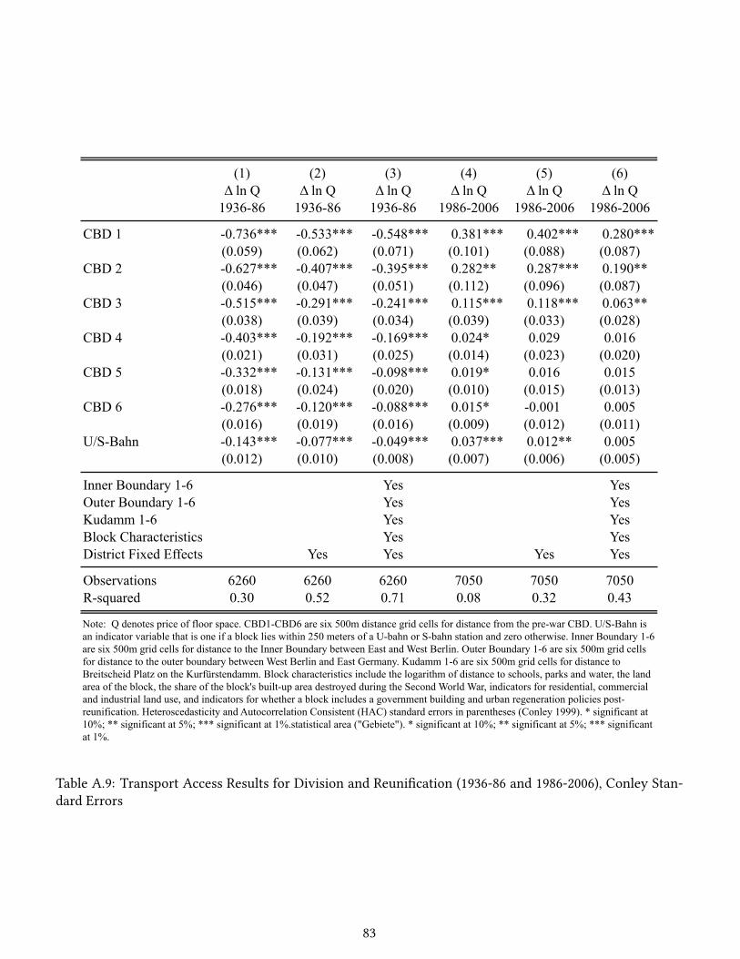
(1) (2) (3) (4) (5) (6)Δ ln Q Δ ln Q Δ ln Q Δ ln Q Δ ln Q Δ ln Q
1936-86 1936-86 1936-86 1986-2006 1986-2006 1986-2006
CBD 1 -0.736*** -0.533*** -0.548*** 0.381*** 0.402*** 0.280***(0.059) (0.062) (0.071) (0.101) (0.088) (0.087)
CBD 2 -0.627*** -0.407*** -0.395*** 0.282** 0.287*** 0.190**(0.046) (0.047) (0.051) (0.112) (0.096) (0.087)
CBD 3 -0.515*** -0.291*** -0.241*** 0.115*** 0.118*** 0.063**(0.038) (0.039) (0.034) (0.039) (0.033) (0.028)
CBD 4 -0.403*** -0.192*** -0.169*** 0.024* 0.029 0.016(0.021) (0.031) (0.025) (0.014) (0.023) (0.020)
CBD 5 -0.332*** -0.131*** -0.098*** 0.019* 0.016 0.015(0.018) (0.024) (0.020) (0.010) (0.015) (0.013)
CBD 6 -0.276*** -0.120*** -0.088*** 0.015* -0.001 0.005(0.016) (0.019) (0.016) (0.009) (0.012) (0.011)
U/S-Bahn -0.143*** -0.077*** -0.049*** 0.037*** 0.012** 0.005(0.012) (0.010) (0.008) (0.007) (0.006) (0.005)
Inner Boundary 1-6 Yes YesOuter Boundary 1-6 Yes YesKudamm 1-6 Yes YesBlock Characteristics Yes YesDistrict Fixed Effects Yes Yes Yes Yes
Observations 6260 6260 6260 7050 7050 7050R-squared 0.30 0.52 0.71 0.08 0.32 0.43
Table A9: Transport Access Results (1936-1986 and 1986-2006, Conley Standard Errors)
Note: Q denotes price of floor space. CBD1-CBD6 are six 500m distance grid cells for distance from the pre-war CBD. U/S-Bahn is an indicator variable that is one if a block lies within 250 meters of a U-bahn or S-bahn station and zero otherwise. Inner Boundary 1-6 are six 500m grid cells for distance to the Inner Boundary between East and West Berlin. Outer Boundary 1-6 are six 500m grid cells for distance to the outer boundary between West Berlin and East Germany. Kudamm 1-6 are six 500m grid cells for distance to Breitscheid Platz on the Kurfürstendamm. Block characteristics include the logarithm of distance to schools, parks and water, the land area of the block, the share of the block's built-up area destroyed during the Second World War, indicators for residential, commercial and industrial land use, and indicators for whether a block includes a government building and urban regeneration policies post-reunification. Heteroscedasticity and Autocorrelation Consistent (HAC) standard errors in parentheses (Conley 1999). * significant at 10%; ** significant at 5%; *** significant at 1%.statistical area ("Gebiete"). * significant at 10%; ** significant at 5%; *** significant at 1%.
Table A.9: Transport Access Results for Division and Reunication (1936-86 and 1986-2006), Conley Stan-dard Errors
83

(1) (2) (3) (4) (5) (6)Δ ln Q Δ ln Q Δ ln Q Δ ln Q Δ ln Q Δ ln Q
1936-86 1936-86 1936-86 1986-2006 1986-2006 1986-2006
CBD 1 -0.736*** -0.533*** -0.548*** 0.381** 0.402*** 0.280**(0.086) (0.094) (0.108) (0.149) (0.125) (0.120)
CBD 2 -0.627*** -0.407*** -0.395*** 0.282* 0.287** 0.190(0.066) (0.069) (0.073) (0.167) (0.136) (0.125)
CBD 3 -0.515*** -0.291*** -0.241*** 0.115** 0.118** 0.063*(0.060) (0.059) (0.064) (0.053) (0.047) (0.033)
CBD 4 -0.403*** -0.192*** -0.169*** 0.024 0.029 0.016(0.031) (0.039) (0.035) (0.019) (0.027) (0.019)
CBD 5 -0.332*** -0.131*** -0.098*** 0.019 0.016 0.015(0.027) (0.029) (0.024) (0.014) (0.017) (0.013)
CBD 6 -0.276*** -0.120*** -0.088*** 0.015 -0.001 0.005(0.031) (0.028) (0.023) (0.013) (0.015) (0.013)
U/S-Bahn -0.143*** -0.077*** -0.049*** 0.037*** 0.012** 0.005(0.019) (0.014) (0.010) (0.008) (0.005) (0.005)
Inner Boundry 1-6 Yes YesOuter Boundary 1-6 Yes YesKudamm 1-6 Yes YesBlock Characteristics Yes YesDistrict Fixed Effects Yes Yes Yes Yes
Observations 6260 6260 6260 7050 7050 7050R-squared 0.30 0.52 0.71 0.08 0.32 0.43
Note: This table reports a robustness test for Table A9 in this web appendix using clustered standard errors. Q denotes price of floor space. CBD1-CBD6 are six 500m distance grid cells for distance from the pre-war CBD. U/S-Bahn is an indicator variable that is one if a block lies within 250 meters of a U-bahn or S-bahn station and zero otherwise. Inner Boundary 1-6 are six 500m grid cells for distance to the Inner Boundary between East and West Berlin. Outer Boundary 1-6 are six 500m grid cells for distance to the outer boundary between West Berlin and East Germany. Kudamm 1-6 are six 500m grid cells for distance to Breitscheid Platz on the Kurfürstendamm. Block characteristics include the logarithm of distance to schools, parks and water, the land area of the block, the share of the block's built-up area destroyed during the Second World War, indicators for residential, commercial and industrial land use, and indicators for whether a block includes a government building and urban regeneration policies post-reunification. Standard errors in parentheses are heteroscedasticity robust and clustered on statistical area (Gebiete). * significant at 10%; ** significant at 5%; *** significant at 1%.statistical area ("Gebiete"). * significant at 10%; ** significant at 5%; *** significant at 1%.
Table A.10: Robustness Test for Transport Access Results for Division and Reunication (1936-86 and 1986-2006), Clustered Standard Errors
84

(1) (2) (3) (4) (5) (6)Δ ln A Δ ln B Δ ln A Δ ln B Δ ln QC Δ ln QC
1936-86 1936-86 1986-2006 1986-2006 1936-1986 1986-2006
CBD 1 -0.207*** -0.347*** 0.261** 0.203*** -0.229*** 0.065***(0.065) (0.089) (0.109) (0.060) (0.013) (0.009)
CBD 2 -0.260*** -0.242*** 0.144** 0.109 -0.184*** 0.065***(0.038) (0.064) (0.071) (0.071) (0.007) (0.007)
CBD 3 -0.138*** -0.262*** 0.077*** 0.059* -0.177*** 0.043***(0.030) (0.037) (0.024) (0.032) (0.008) (0.007)
CBD 4 -0.131*** -0.154*** 0.057*** 0.010 -0.189*** 0.048***(0.015) (0.031) (0.016) (0.010) (0.006) (0.005)
CBD 5 -0.095*** -0.126*** 0.028** -0.014 -0.188*** 0.055***(0.016) (0.020) (0.013) (0.010) (0.006) (0.006)
CBD 6 -0.061*** -0.117*** 0.023** 0.001 -0.170*** 0.035***(0.021) (0.026) (0.010) (0.006) (0.005) (0.004)
Counterfactuals Yes YesAgglomeration Effects No No
Observations 2844 5978 5602 6718 6260 7050R-squared 0.09 0.06 0.02 0.03 0.10 0.07
Note: This table reports a robustness test for Table 4 in the paper using clustered standard errors. Columns (1)-(4) based on calibrating the model for ν=εκ=0.07 and ε=6.83 from the gravity equation estimation. Columns (5)-(6) report counterfactuals for these parameter values. A denotes adjusted overall productivity. B denotes adjusted overall amenities. QC denotes counterfactual floor prices (simulating the effect of division on West Berlin). Column (5) simulates division holding A and B constant at their 1936 values. Column (6) simulates reunification holding A and B for West Berlin constant at their 1986 values and using 1936 values of A and B for East Berlin. CBD1-CBD6 are six 500m distance grid cells for distance from the pre-war CBD. Robust Standard Errors in Parentheses adjusted for clustering by statistical area ("Gebiete"). * significant at 10%; ** significant at 5%; *** significant at 1%.
Table A.11: Robustness Test for Floor Prices, Productivity and Amenities, Clustered Standard Errors
85
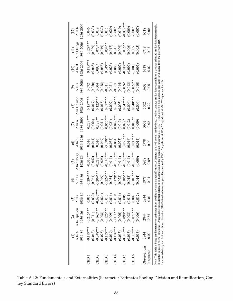
(1)
(2)
(3)
(4)
(5)
(6)
(7)
(8)
(9)
(10)
(11)
(12)
Δ ln
AΔ
ln U
psilo
nΔ
ln a
Δ ln
BΔ
ln O
meg
aΔ
ln b
Δ ln
AΔ
ln U
psilo
nΔ
ln a
Δ ln
BΔ
ln O
meg
aΔ
ln b
1936
-86
1936
-86
1936
-86
1936
-86
1936
-86
1936
-198
619
86-2
006
1986
-200
619
86-2
006
1986
-200
619
86-2
006
1986
-200
6
CB
D 1
-0
.199
***
-0
.215
***
0.01
6
-0.2
94**
*
-0.3
10**
*0.
016
0
.229
***
0
.157
***
0.07
2
0.1
75**
*
0.1
29**
*0.
046
(0.0
43)
(0.0
11)
(0.0
39)
(0.0
63)
(0.0
42)
(0.0
41)
(0.0
64)
(0.0
17)
(0.0
50)
(0.0
48)
(0.0
29)
(0.0
33)
CB
D 2
-0
.248
***
-0
.162
***
-0
.086
***
-0
.204
***
-0
.213
***
0.01
0
0.12
7**
0
.123
***
0.00
40.
092*
0
.073
***
0.01
9(0
.028
)(0
.008
)(0
.024
)(0
.049
)(0
.025
)(0
.049
)(0
.051
)(0
.018
)(0
.038
)(0
.053
)(0
.019
)(0
.037
)C
BD
3
-0.1
39**
*
-0.1
25**
*-0
.013
-0.2
24**
*
-0.1
46**
* -
0.07
8**
0
.066
***
0
.077
***
-0.0
11
0.
049*
*
0.03
4**
0.01
5(0
.019
)(0
.009
)(0
.016
)(0
.034
)(0
.011
)(0
.033
)(0
.021
)(0
.007
)(0
.021
)(0
.023
)(0
.017
)(0
.029
)C
BD
4
-0.1
30**
*
-0.1
11**
*-0
.019
-0.1
29**
*
-0.1
28**
*-0
.001
0.0
48**
*
0.0
56**
*-0
.007
0.
005
0.01
1-0
.007
(0
.015
)(0
.006
)(0
.016
)(0
.022
)(0
.011
)(0
.025
)(0
.013
)(0
.003
)(0
.014
)(0
.007
)(0
.009
)(0
.010
)C
BD
5
-0.0
95**
*
-0.0
90**
*-0
.005
-0.1
05**
*
-0.1
56**
*
0.0
51**
* 0
.022
*
0.0
47**
*-0
.024
* -
0.01
7**
0.
015*
*
-0.0
32**
*(0
.013
)(0
.008
)(0
.011
)(0
.013
)(0
.011
)(0
.016
)(0
.012
)(0
.004
)(0
.013
)(0
.007
)(0
.006
)(0
.009
)C
BD
6
-0.0
62**
*
-0.0
71**
*0.
009
-0
.101
***
-0
.139
***
0
.037
***
0.
018*
*
0.0
40**
* -
0.02
2**
-0.0
03
0.00
5-0
.007
(0
.013
)(0
.006
)(0
.012
)(0
.014
)(0
.009
)(0
.014
)(0
.009
)(0
.004
)(0
.010
)(0
.005
)(0
.005
)(0
.007
)
Obs
erva
tions
2844
2844
2844
5978
5978
5978
5602
5602
5602
6718
6718
6718
R-s
quar
ed0.
090.
350.
010.
040.
090.
000.
020.
220.
000.
020.
030.
00
Tabl
e A12
: Fun
dam
enta
ls a
nd E
xter
nalit
ies (
Con
ley
Stan
dard
Err
ors)
Not
e: T
his t
able
is b
ased
on
the
para
met
er e
stim
ates
from
poo
ling
divi
sion
and
reun
ifica
tion.
A d
enot
es a
djus
ted
over
all p
rodu
ctiv
ity. U
psilo
n de
note
s pro
duct
ion
exte
rnal
ities
. a d
enot
es a
djus
ted
prod
uctio
n fu
ndam
enta
ls.
B d
enot
es a
djus
ted
over
all a
men
ities
. Om
ega
deno
tes r
esid
entia
l ext
erna
litie
s. b
deno
tes a
djus
ted
prod
uctio
n fu
ndam
enta
ls. C
BD
1-C
BD
6 ar
e si
x 50
0m d
ista
nce
grid
cel
ls fo
r dis
tanc
e fr
om th
e pr
e-w
ar C
BD
. H
eter
osce
dast
icity
and
Aut
ocor
rela
tion
Con
sist
ent (
HA
C) s
tand
ard
erro
rs in
par
enth
eses
(Con
ley
1999
). *
sign
ifica
nt a
t 10%
; **
sign
ifica
nt a
t 5%
; ***
sign
ifica
nt a
t 1%
.
Table A.12: Fundamentals and Externalities (Parameter Estimates Pooling Division and Reunication, Con-ley Standard Errors)
86

(1)
(2)
(3)
(4)
(5)
(6)
(7)
(8)
(9)
(10)
(11)
(12)
Δ ln
AΔ
ln U
psilo
nΔ
ln a
Δ ln
BΔ
ln O
meg
aΔ
ln b
Δ ln
AΔ
ln U
psilo
nΔ
ln a
Δ ln
BΔ
ln O
meg
aΔ
ln b
1936
-86
1936
-86
1936
-86
1936
-86
1936
-86
1936
-198
619
86-2
006
1986
-200
619
86-2
006
1986
-200
619
86-2
006
1986
-200
6
CB
D 1
-0
.199
***
-0
.215
***
0.01
6
-0.2
94**
*
-0.3
10**
*0.
016
0.
229*
*
0.1
57**
*0.
072
0
.175
***
0
.129
***
0.
046*
*(0
.056
)(0
.016
)(0
.044
)(0
.081
)(0
.050
)(0
.033
)(0
.096
)(0
.023
)(0
.074
)(0
.054
)(0
.036
)(0
.018
)C
BD
2
-0.2
48**
*
-0.1
62**
*
-0.0
86**
*
-0.2
04**
*
-0.2
13**
*0.
010
0.12
7*
0.1
23**
*0.
004
0.09
2
0.0
73**
*0.
019
(0.0
35)
(0.0
12)
(0.0
24)
(0.0
61)
(0.0
40)
(0.0
55)
(0.0
65)
(0.0
28)
(0.0
41)
(0.0
64)
(0.0
22)
(0.0
44)
CB
D 3
-0
.139
***
-0
.125
***
-0.0
13
-0
.224
***
-0
.146
***
-0.
078*
*
0.0
66**
*
0.0
77**
*-0
.011
0
.049
* 0
.034
*0.
015
(0.0
28)
(0.0
14)
(0.0
18)
(0.0
39)
(0.0
14)
(0.0
38)
(0.0
22)
(0.0
07)
(0.0
20)
(0.0
29)
(0.0
20)
(0.0
35)
CB
D 4
-0
.130
***
-0
.111
***
-0.0
19
-0
.129
***
-0
.128
***
-0.0
01
0
.048
***
0
.056
***
-0.0
07
0.00
50.
011
-0.0
07
(0.0
15)
(0.0
09)
(0.0
15)
(0.0
33)
(0.0
16)
(0.0
33)
(0.0
15)
(0.0
05)
(0.0
16)
(0.0
10)
(0.0
11)
(0.0
12)
CB
D 5
-0
.095
***
-0
.090
***
-0.0
05
-0
.105
***
-0
.156
***
0.
051*
* 0
.022
*
0.0
47**
*-0
.024
*-0
.017
0
.015
* -
0.03
2**
(0.0
15)
(0.0
11)
(0.0
13)
(0.0
24)
(0.0
17)
(0.0
22)
(0.0
12)
(0.0
06)
(0.0
13)
(0.0
10)
(0.0
08)
(0.0
12)
CB
D 6
-0
.062
***
-0
.071
***
0.00
9
-0.1
01**
*
-0.1
39**
* 0
.037
*
0.01
8**
0
.040
***
-0.0
22*
-0.0
03
0.00
5-0
.007
(0
.020
)(0
.009
)(0
.019
)(0
.029
)(0
.019
)(0
.021
)(0
.009
)(0
.006
)(0
.011
)(0
.006
)(0
.006
)(0
.009
)
Obs
erva
tions
2844
2844
2844
5978
5978
5978
5602
5602
5602
6718
6718
6718
R-s
quar
ed0.
090.
350.
010.
040.
090.
000.
020.
220.
000.
020.
030.
00
Not
e: T
his t
able
is b
ased
on
the
para
met
er e
stim
ates
from
poo
ling
divi
sion
and
reun
ifica
tion.
A d
enot
es a
djus
ted
over
all p
rodu
ctiv
ity. U
psilo
n de
note
s pro
duct
ion
exte
rnal
ities
. a d
enot
es a
djus
ted
prod
uctio
n fu
ndam
enta
ls.
B d
enot
es a
djus
ted
over
all a
men
ities
. Om
ega
deno
tes r
esid
entia
l ext
erna
litie
s. b
deno
tes a
djus
ted
prod
uctio
n fu
ndam
enta
ls. C
BD
1-C
BD
6 ar
e si
x 50
0m d
ista
nce
grid
cel
ls fo
r dis
tanc
e fr
om th
e pr
e-w
ar C
BD
. Rob
ust
Stan
dard
Err
ors i
n Pa
rent
hese
s adj
uste
d fo
r clu
ster
ing
by st
atis
tical
are
a ("
Geb
iete
"). *
sign
ifica
nt a
t 10%
; **
sign
ifica
nt a
t 5%
; ***
sign
ifica
nt a
t 1%
.
Table A.13: Robustness Test for Fundamentals and Externalities (Parameter Estimates Pooling Division andReunication, Clustered Standard Errors)
87
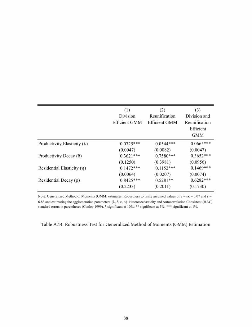
(1) (2) (3)Division
Efficient GMMReunification
Efficient GMMDivision and Reunification
Efficient GMM
Productivity Elasticity (λ) 0.0725*** 0.0544*** 0.0665***(0.0047) (0.0082) (0.0047)
Productivity Decay (δ) 0.3621*** 0.7580*** 0.3652***(0.1250) (0.3981) (0.0956)
Residential Elasticity (η) 0.1472*** 0.1152*** 0.1469***(0.0064) (0.0207) (0.0074)
Residential Decay (ρ) 0.8425*** 0.5281** 0.6282***(0.2233) (0.2011) (0.1730)
Note: Generalized Method of Moments (GMM) estimates. Robustness to using assumed values of ν = εκ = 0.07 and ε = 6.83 and estimating the agglomeration parameters λ, δ, ε, ρ. Heteroscedasticity and Autocorrelation Consistent (HAC) standard errors in parentheses (Conley 1999). * significant at 10%; ** significant at 5%; *** significant at 1%.
Table A.14: Robustness Test for Generalized Method of Moments (GMM) Estimation
88

(1) (2)
ln Model Density of Development 2006
ln Model Density of Development 2006
ln Data Density of Development 2006 0.9610*** 0.9610***(0.0296) (0.0181)
Standard Errors Conley ClusteredObservations 7050 7050R-squared 0.37 0.37
Note: The table is based on the parameter estimates pooling division and reunification from Table 5 of the paper. The dependent variable is the logarithm of the adjusted density of development in the model (varphi) for 2006. The independent variable is the logarithm of the ratio of floor space to geographical land area (GFZ) in the data for 2006. Column (1) reports Heteroscedasticity and Autocorrelation Consistent (HAC) standard errors following Conley (1999). Column (2) reports standard errors clustered by statistical area ("Gebiet"). * significant at 10%; ** significant at 5%; *** significant at 1%.
Table A.15: Density of Development Overidentication Check
89

(1) (2) (3) (4)ln Production Fundamental
2006
ln Residential Fundamental
2006
ln Production Fundamental
2006
ln Residential Fundamental
2006
Green Areas 0.0061*** 0.0185*** 0.0061*** 0.0185***(0.0007) (0.0010) (0.0009) (0.0014)
Water Areas 0.0440*** 0.0487*** 0.0440*** 0.0487***(0.0066) (0.0109) (0.0093) (0.0174)
War Destruction -0.0356 -0.1935*** -0.0356 -0.1935***(0.0151) (0.0232) (0.0222) (0.0407)
Listed Buildings 0.0503*** 0.0195*** 0.0503*** 0.0195***(0.0032) (0.0047) (0.0042) (0.0054)
Noise 0.0062 -0.2869*** 0.0062 -0.2869***(0.0201) (0.0286) (0.0356) (0.0510)
Standard Errors Conley Conley Clustered ClusteredObservations 0.123 0.218 0.123 0.218R-squared 9437 11863 9437 11863
Note: This table is based on the parameter estimates pooling division and reunification from Table 5 in the paper. The dependent variable in Columns (1) and (3) is the log adjusted production fundamental in the model (a) for 2006. The dependent variable in Columns (2) and (4) is the log adjusted residential fundamental in the model (b) in 2006. The independent variable is the log ratio of floor space to geographical land area (GFZ) in the data for 2006. Green Areas are the logarithm of one plus the square meters of green areas in a block; Water Areas is a dummy which is one if the block is adjacent to a lake, river or canal; War Destruction is the share of the block's built-up area that was destroyed during the Second World War; Listed Buildings is the logarithm of one plus the number of listed buildings in a block; Noise is the logarithm of the average noise level in decibel in a block; Columns (1) and (2) report Heteroscedasticity and Autocorrelation Consistent (HAC) standard errors following Conley (1999). Columns (3) and (4) report standard errors clustered by statistical area ("Gebiet"). * significant at 10%; ** significant at 5%; *** significant at 1%.
Table A.16: Production and Residential Fundamentals Overidentication Check
90

(1) (2) (3) (4) (5) (6)Δ ln QC Δ ln QC Δ ln QC Δ ln QC Δ ln QC Δ ln QC1936-86 1936-86 1936-86 1936-1986 1986-2006 1936-1986
CBD 1 -0.839*** -0.667*** -0.666*** -0.752*** 0.472*** 0.923***(0.055) (0.031) (0.050) (0.030) (0.048) (0.056)
CBD 2 -0.627*** -0.456*** -0.635*** -0.585*** 0.251*** 0.689***(0.038) (0.019) (0.044) (0.022) (0.045) (0.064)
CBD 3 -0.518*** -0.348*** -0.592*** -0.476*** 0.086** 0.416***(0.044) (0.017) (0.059) (0.023) (0.041) (0.042)
CBD 4 -0.521*** -0.329*** -0.642*** -0.470*** -0.060** 0.311***(0.039) (0.012) (0.052) (0.022) (0.030) (0.034)
CBD 5 -0.544*** -0.306*** -0.733*** -0.482*** -0.076*** 0.253***(0.028) (0.012) (0.036) (0.019) (0.027) (0.030)
CBD 6 -0.489*** -0.265*** -0.709*** -0.417*** -0.133*** 0.163***(0.024) (0.008) (0.034) (0.015) (0.025) (0.026)
Counterfactuals Yes Yes Yes Yes Yes YesAgglomeration Effects Yes Yes Yes Yes Yes Yes
Observations 6260 6260 6260 6260 7050 6260R-squared 0.12 0.15 0.08 0.11 0.01 0.06
Note: This table is based on the parameter estimates pooling division and reunification from Table 5 in the paper. QC denotes counterfactual floor prices. Column (1) simulates division using our estimates of production and residential externalities and 1936 fundamentals. Column (2) simulates division using our estimates of production externalities and 1936 fundamentals but setting residential externalities to zero. Column (3) simulates division using our estimates of residential externalities and 1936 fundamentals but setting production externalities to zero. Column (4) simulates division using our estimates of production and residential externalities and 1936 fundamentals but halving their rates of spatial decay with travel time. Column (5) simulates reunification using our estimates of production and residential externalities, 1986 fundamentals for West Berlin, and 2006 fundamentals for East Berlin. Column (6) simulates reunification using our estimates of production and residential externalities, 1986 fundamentals for West Berlin and 1936 fundamentals for East Berlin. CBD1-CBD6 are six 500m distance grid cells for distance from the pre-war CBD. Robust Standard Errors in Parentheses adjusted for clustering by statistical area ("Gebiete"). * significant at 10%; ** significant at 5%; *** significant at 1%.
Table A.17: Robustness Test for Counterfactuals, Clustered Standard Errors
91

Coefficient Standard Error
Year: 2000 -0.073*** (0.020)Year: 2001 -0.105*** (0.021)Year: 2002 -0.142*** (0.020)Year: 2003 -0.176*** (0.019)Year: 2004 -0.193*** (0.020)Year: 2005 -0.124*** (0.017)Year: 2007 0.082*** (0.017)Year: 2008 -0.004 (0.017)Year: 2009 -0.014 (0.019)Year: 2010 0.065*** (0.018)Year: 2011 0.203*** (0.018)Year: 2012 0.279*** (0.023)Age cohort: 5 to 15 years -0.297*** (0.031)Age cohort: 15 to 25 years -0.569*** (0.035)Age cohort: 25 to 35 years -0.783*** (0.035)Age cohort: 35 to 45 years -1.014*** (0.036)Age cohort: 45 to 55 years -1.155*** (0.038)Age cohort: 55 to 65 years -1.021*** (0.039)Age cohort: 65 to 75 years -0.988*** (0.033)Age cohort: 75 to 85 years -1.058*** (0.035)Age cohort: 85 to 95 years -0.967*** (0.039)Age cohort: 95 to 105 years -0.822*** (0.039)Age cohort: 105 to 115 years -0.823*** (0.042)Age cohort: 115 to 125 years -0.859*** (0.048)Age cohort: 125 to 135 years -0.892*** (0.070)Age cohort: 135 to 145 years -0.883*** (0.071)Age cohort: 145 to 155 years -0.854*** (0.135)Age cohort: 155 to 165 years -1.419*** (0.206)Age cohort: 165 to 175 years -1.481*** (0.509)Age cohort: 175 to 185 years -0.430 (0.314)Age cohort: 185 to 195 years -0.607*** (0.115)Age cohort: 195 to 205 years -0.811* (0.462)Age cohort: 205 to 215 years -0.619** (0.306)
Block fixed effectsR-squaredObservations
0.76951,275
Note: This table reports the results of estimating a Case-Shiller type repeated sales specification at the block level using the micro data on property transactions from 2000-2012. Standard errors in parentheses are heteroscedasticity robust and clustered by block. * significant at 10%; ** significant at 5%; *** significant at 1%.
ln(Transaction Price/Lot size)
Yes
Table A.18: Micro Data on Property Transactions
92