matias d. cattaneo department of economics, …econ.msu.edu/seminars/docs/matias...

Bootstrapping Density-Weighted Average Derivatives∗

Matias D. Cattaneo

Department of Economics, University of Michigan

Richard K. Crump

Federal Reserve Bank of New York

Michael Jansson

Department of Economics, UC Berkeley and CREATES

May 17, 2010

Abstract. Employing the “small bandwidth” asymptotic framework of Cat-

taneo, Crump, and Jansson (2009), this paper studies the properties of a variety of

bootstrap-based inference procedures associated with the kernel-based density-weighted

averaged derivative estimator proposed by Powell, Stock, and Stoker (1989). In many

cases validity of bootstrap-based inference procedures is found to depend crucially on

whether the bandwidth sequence satisfies a particular (asymptotic linearity) condition.

An exception to this rule occurs for inference procedures involving a studentized esti-

mator employing a “robust” variance estimator derived from the “small bandwidth”

asymptotic framework. The results of a small-scale Monte Carlo experiment are found

to be consistent with the theory and indicate in particular that sensitivity with respect

to the bandwidth choice can be ameliorated by using the “robust”variance estimator.

Keywords: Averaged derivatives, Bootstrap, Small bandwidth asymptotics.

JEL: C12, C14, C21, C24.

∗The authors thank Joel Horowitz, Lutz Kilian, Demian Pouzo, Rocio Titiunik, and seminar partici-

pants at Duke, Harvard, Michigan, Northwestern and Rochester for comments. The first author gratefully

acknowledges financial support from the National Science Foundation (SES 0921505). The third author

gratefully acknowledges financial support from the National Science Foundation (SES 0920953) and the

research support of CREATES (funded by the Danish National Research Foundation).

1

Bootstrapping Density-Weighted Average Derivatives 2

1. Introduction

Semiparametric estimators involving functionals of nonparametric estimators have been stud-

ied widely in econometrics. In particular, considerable effort has been devoted to charac-

terizing conditions under which such estimators are asymptotically linear (see, e.g., Newey

and McFadden (1994), Chen (2007), and the references therein). Moreover, although the

asymptotic variance of an asymptotically linear semiparametric estimator can in principle

be obtained by means of the pathwise derivative formula of Newey (1994a), it is desirable

from a practical point of view to be able to base inference procedures on measures of disper-

sion that are “automatic”in the sense that they can be constructed without knowledge (or

derivation) of the influence function (e.g., Newey (1994b)).

Perhaps the most natural candidates for such measures of dispersion are variances and/or

percentiles obtained using the bootstrap.1 Consistency of the nonparametric bootstrap has

been established for a large class of semiparametric estimators by Chen, Linton, and van

Keilegom (2003). Moreover, in the important special case of the density-weighted average

derivative estimator of Powell, Stock, and Stoker (1989, henceforth PSS), a suitably im-

plemented version of the nonparametric bootstrap was shown by Nishiyama and Robinson

(2005, henceforth NR) to provide asymptotic refinements. The analysis in NR is conducted

within the asymptotic framework of Nishiyama and Robinson (2000, 2001). Using the al-

ternative asymptotic framework of Cattaneo, Crump, and Jansson (2009, henceforth CCJ),

this paper revisits the large sample behavior of bootstrap-based inference procedures for

density-weighted average derivatives and obtains (analytical and Monte Carlo) results that

could be interpreted as a cautionary tale regarding the ease with which one might realize

“the potential for bootstrap-based inference to (...) provide improvements in moderate-sized

samples”(NR, p. 927).

Because the influence function of an asymptotically linear semiparametric estimator is

invariant with respect to the nonparametric estimator upon which it is based (e.g., Newey

(1994a, Proposition 1)), looking beyond the influence function is important if the sensitivity

of the distributional properties of an estimator or test statistic with respect to user chosen

objects such as kernels or bandwidths is a concern. This can be accomplished in various ways,

the traditional approach being to work under assumptions that imply asymptotic linearity

and then develop asymptotic expansions (of the Edgeworth or Nagar variety) intended to

1Another “automatic”measure of dispersion is the variance estimator of Newey (1994b). When appliedto the density-weighted average derivative estimator studied in this paper, the variance estimator of Newey(1994b) coincides with Powell, Stock, and Stoker’s (1989) variance estimator whose salient properties arecharacterized in Lemma 1 below.


elucidate the role of “higher-order”terms (e.g., Linton (1995)). Similarly to the Edgeworth

expansions employed by Nishiyama and Robinson (2000, 2001, 2005), CCJ’s asymptotic dis-

tribution theory for PSS’s estimator (and its studentized version) is obtained by retaining

terms that are asymptotically negligible when the estimator is asymptotically linear. Unlike

the traditional approach, the “small bandwidth” approach taken by CCJ accommodates,

but does not require, certain departures from asymptotic linearity, namely those that occur

when the bandwidth of the nonparametric estimator vanishes too rapidly for asymptotic lin-

earity to hold. Although similar in spirit to the Edgeworth expansion approach to improved

asymptotic approximations, the small bandwidth approach of CCJ is conceptually distinct

from the approach taken by Nishiyama and Robinson (2000, 2001, 2005) and it is therefore

of interest to explore whether the small bandwidth approach gives rise to methodological

prescriptions that differ from those obtained using the traditional approach.

The first main result, Theorem 1 below, studies the validity of bootstrap-based approxi-

mations to the distribution of PSS’s estimator as well as its studentized version in the case

where PSS’s variance estimator is used for studentization purposes. It is shown that a nec-

essary condition for bootstrap consistency is that the bandwidth vanishes slowly enough for

asymptotic linearity to hold. Unlike NR, Theorem 1 therefore suggests that in samples of

moderate size even the bootstrap approximations to the distributions of PSS’s estimator and

test statistic(s) may fail to adequately capture the extent to which these distributions are

affected by the choice of the bandwidth, a prediction which is borne out in a small scale

Monte Carlo experiment reported in Section 4.

The second main result, Theorem 2, establishes consistency of the bootstrap approxi-

mation to the distribution of PSS’s estimator studentized by means of a variance estimator

proposed by CCJ. As a consequence, Theorem 2 suggests that the fragility with respect to

bandwidth choice uncovered by Theorem 1 is a property which should be attributed to PSS’s

variance estimator rather than the bootstrap distribution estimator. Another prediction of

Theorem 2, namely that the bootstrap approximation to the distribution of an appropriately

studentized estimator performs well across a wide range of bandwidths, is borne out in the

Monte Carlo experiment of Section 4. Indeed, the range of bandwidths across which the

bootstrap is found to perform well is wider than the range across which the standard normal

approximation is found to perform well, indicating that there is an important sense in which

bootstrap-based inference is capable of providing improvements in moderate-sized samples.

The variance estimator used for studentization purposes in Theorem 2 is one for which the

studentized estimator is asymptotically standard normal across the entire range of bandwidth


sequences considered in CCJ’s approach. The final main result, Theorem 3, studies the

bootstrap approximation to the distribution of PSS’s estimator studentized by means of

an alternative variance estimator also proposed by CCJ and finds, perhaps surprisingly,

that although the associated studentized estimator is asymptotically standard normal across

the entire range of bandwidth sequences considered in CCJ’s approach, consistency of the

bootstrap requires that the bandwidth vanishes slowly enough for asymptotic linearity to

hold.

In addition to NR, whose relation to the present work was discussed in some detail above,

the list of papers related to this paper includes Abadie and Imbens (2008) and Gonçalves

and Vogelsang (2010). Abadie and Imbens (2008) study a nearest-neighbor matching esti-

mator of a popular estimand in the program evaluation literature (the effect of treatment

on the treated) and demonstrate by example that the nonparametric bootstrap variance

estimator can be inconsistent in that case. Although the nature of the nonparametric es-

timator employed by Abadie and Imbens (2008) differs from the kernel estimator studied

herein, their inconsistency result would appear to be similar to the equivalence between

(i) and (ii) in Theorem 1(a) below. Comparing the results of this paper with those ob-

tained by Abadie and Imbens (2008), one apparent attraction of kernel estimators (relative

to nearest-neighbor estimators) is their tractability which allows to develop fairly detailed

characterizations of the large-sample behavior of bootstrap procedures, including an array of

(constructive) results on how to achieve bootstrap consistency even under departures from

asymptotic linearity. Gonçalves and Vogelsang (2010) are concerned with autocorrelation

robust inference in stationary regression models and establish consistency of the bootstrap

under the fixed-b asymptotics of Kiefer and Vogelsang (2005). Although the fixed-b approach

of Kiefer and Vogelsang (2005) is very similar in spirit to the “small bandwidth”approach of

CCJ, the fact that some of the results of this paper are invalidity results about the bootstrap

is indicative of an important difference between the nature of the functionals being studied

in Kiefer and Vogelsang (2005) and CCJ, respectively.

The remainder of the paper is organized as follows. Section 2 introduces the model,

presents the statistics under consideration, and summarizes some results available in the

literature. Section 3 studies the bootstrap and obtains the main results of the paper. Section

4 summarizes the results of a simulation study. Section 5 concludes. The Appendix contains

proofs of the theoretical results.


2. Model and Existing Results

Let Zn = zi = (yi, x′i)′ : i = 1, . . . , n be a random sample of the random vector z = (y, x′)′,

where y ∈ R is a dependent variable and x ∈ Rd is a continuous explanatory variable witha density f (·). The density-weighted average derivative is given by

θ = E[f (x)

∂

∂xg (x)

], g (x) = E [y|x] .

It follows from (regularity conditions and) integration by parts that θ = −2E [y ∂f (x)/ ∂x].

Noting this, PSS proposed the kernel-based estimator

θn = −21

n

n∑i=1

yi∂

∂xfn,i (xi) , fn,i (x) =

1

n− 1

n∑j=1,j 6=i

1

hdnK

(xj − xhn

),

where fn,i (·) is a “leave-one-out”estimator of f (·), with K : Rd → R a kernel function andhn a positive (bandwidth) sequence.

To analyze inference procedures based on θn, some assumptions on the distribution of z

and the properties of the user-chosen ingredients K and hn are needed. Regarding the model

and kernel function, the following assumptions will be made.

Assumption M. (a) E[y4] < ∞, E [σ2 (x) f (x)] > 0 and V [∂e (x) /∂x− y∂f (x) /∂x] is

positive definite, where σ2 (x) = V [y|x] and e (x) = f (x) g (x).

(b) f is (Q+ 1) times differentiable, and f and its first (Q+ 1) derivatives are bounded,

for some Q ≥ 2.

(c) g is twice differentiable, and e and its first two derivatives are bounded.

(d) v is differentiable, and vf and its first derivative are bounded, where v (x) = E[y2|x].

(e) lim‖x‖→∞ [f (x) + |e (x)|] = 0, where ‖·‖ is the Euclidean norm.

Assumption K. (a)K is even and differentiable, andK and its first derivative are bounded.

(b)∫Rd K (u) K (u)′du is positive definite, where K (u) = ∂K (u) /∂u.

(c) For some P ≥ 2,∫Rd |K (u)| (1 + ‖u‖P )du+

∫Rd ‖K (u) ‖(1 + ‖u‖2)du <∞, and

∫Rdul11 · · ·u

ldd K (u)du =

1, if l1 = · · · = ld = 0,

0, if (l1, . . . , ld)′ ∈ Zd+ and l1 + · · ·+ ld < P

.

The following conditions on the bandwidth sequence hn will play a crucial role in the sequel.

(Here, and elsewhere in the paper, limits are taken as n→∞ unless otherwise noted.)


Condition B. (Bias) min(nhd+2

n , 1)nh

2 min(P,Q)n → 0.

Condition AL. (Asymptotic Linearity) nhd+2n →∞.

Condition AN. (Asymptotic Normality) n2hdn →∞.

PSS studied the large sample properties of θn and showed that if Assumptions M and K

hold and if Conditions B and AL are satisfied, then θn is asymptotically linear with (effi cient)

influence function L (z) = 2 [∂e (x)/ ∂x− y ∂f (x)/ ∂x− θ]; that is,

√n(θn − θ) =

1√n

n∑i=1

L (zi) + op (1) N (0,Σ) , Σ = E[L (z)L (z)′

], (1)

where denotes weak convergence. PSS’s derivation of this result exploits the fact that the

estimator θn admits the (n-varying) U -statistic representation θn = θn(hn) with

θn(h) =

(n

2

)−1 n−1∑i=1

n∑j=i+1

U (zi, zj;h) , U (zi, zj;h) = −h−(d+1)K

(xi − xjh

)(yi − yj) ,

which leads to the Hoeffding decomposition θn − θ = Bn + Ln + Wn, where

Bn = θ (hn)− θ, Ln = n−1

n∑i=1

L (zi;hn) , Wn =

(n

2

)−1 n−1∑i=1

n∑j=i+1

W (zi, zj;hn),

with

θ (h) = E [U (zi, zj;h)] , L (zi;h) = 2 [E[U (zi, zj;h) |zi]− θ (h)] ,

W (zi, zj;h) = U (zi, zj;h)− 1

2(L (zi;h) + L (zj;h))− θ (h) .

The purpose of Conditions B and AL is to ensure that the terms Bn and Wn in the Ho-

effding decomposition are asymptotically negligible. Specifically, because Bn = O(hmin(P,Q)n )

under Assumptions M and K, Condition B ensures that the bias of θn is asymptotically

negligible. Condition AL, on the other hand, ensures that the “quadratic”term Wn in the

Hoeffding decomposition is asymptotically negligible because√nWn = Op(1/

√nhd+2

n ) under

Assumptions M and K. In other words, and as the notation suggests, Condition AL is crucial

for asymptotic linearity of θn.

While asymptotic linearity is a desirable feature from the point of view of asymptotic effi -

ciency, a potential concern about distributional approximations for θn based on assumptions


which imply asymptotic linearity is that such approximations ignore the variability in the

“remainder”term Wn. Thus, classical first-order, asymptotically linear, large sample theory

may not accurately capture the finite sample behavior of θn in general. It therefore seems

desirable to employ inference procedures that are “robust” in the sense that they remain

asymptotically valid at least under certain departures from asymptotic linearity.

In an attempt to construct such inference procedures, CCJ generalized (1) and showed

that if Assumptions M and K hold and if Conditions B and AN are satisfied, then

V −1/2n (θn − θ) N (0, Id) , (2)

where

Vn = n−1Σ +

(n

2

)−1

h−(d+2)n ∆, ∆ = 2E

[σ2 (x) f (x)

] ∫RdK (u) K (u)′ du.

Similarly to the asymptotic linearity result of PSS, the derivation of (2) is based on the

Hoeffding decomposition of θn. Instead of requiring asymptotic linearity of the estimator,

this result provides an alternative first-order asymptotic theory under weaker assumptions,

which simultaneously accounts for both the “linear”and “quadratic”terms in the expansion

of θn. A key difference between (1) and (2) is the presence of the term(n2

)−1h−(d+2)n ∆ in

Vn, which captures the variability of Wn. In particular, result (2) shows that while failure

of Condition AL leads to a failure of asymptotic linearity, asymptotic normality of θn holds

under the significantly weaker Condition AN.2

The result (2) suggests that asymptotic standard normality of studentized estimators

might be achievable also when Condition AL is replaced by Condition AN. As an estimator

of the variance of θn, PSS considered V0,n = n−1Σn, where Σn = Σn(hn),

Σn(h) =1

n

n∑i=1

Ln,i(h)Ln,i(h)′, Ln,i(h) = 2

[1

n− 1

n∑j=1,j 6=i

U(zi, zj;h)− θn(h)

].

CCJ showed that this estimator admits the stochastic expansion

V0,n = n−1 [Σ + op (1)] + 2

(n

2

)−1

h−(d+2)n [∆ + op (1)] ,

2Condition AN permits failure not only of asymptotic linearity, but also of√n-consistency (when nhd+2n →

0). Indeed, θn can be inconsistent (when limn→∞n2hd+2n <∞) under Condition AN.


implying in particular that it is consistent only when Condition AL is satisfied. Recognizing

this lack of “robustness” of V0,n with respect to hn, CCJ proposed and studied the two

alternative estimators

V1,n = V0,n −(n

2

)−1

h−(d+2)n ∆n(hn) and V2,n = n−1Σn(21/(d+2)hn),

where

∆n(h) = hd+2

(n

2

)−1 n−1∑i=1

n∑j=i+1

Wn,ij(h)Wn,ij(h)′,

Wn,ij(h) = U(zi, zj;h)− 1

2

(Ln,i(h) + Ln,j(h)

)− θn(h).

The following result is adapted from CCJ and formulated in a manner that facilitates

comparison with the main theorems given below.

Lemma 1. Suppose Assumptions M and K hold and suppose Conditions B and AN are

satisfied.

(a) The following are equivalent:

i. Condition AL is satisfied.

ii. V −1n V0,n →p Id.

iii. V−1/2

0,n (θn − θ) N (0, Id).

(b) If nhd+2n is convergent in R+ = [0,∞], then V

−1/20,n (θn − θ) N (0,Ω0), where

Ω0 = limn→∞(nhd+2n Σ + 4∆)−1/2(nhd+2

n Σ + 2∆)(nhd+2n Σ + 4∆)−1/2.

(c) For k ∈ 1, 2, V −1n Vk,n →p Id and V

−1/2k,n (θn − θ) N (0, Id).

Part (a) is a qualitative result highlighting the crucial role played by Condition AL in

connection with asymptotic validity of inference procedures based on V0,n. The equivalence

between (i) and (iii) shows that Condition AL is necessary and suffi cient for the test statistic

V−1/2

0,n (θn − θ) proposed by PSS to be asymptotically pivotal. In turn, this equivalence is

a special case of part (b), which is a quantitative result that can furthermore be used to

characterize the consequences of relaxing Condition AL. Specifically, part (b) shows that


also under departures from Condition AL the statistic V−1/2

0,n (θn − θ) can be asymptoticallynormal with mean zero, but with a variance matrix Ω0 whose value depends on the limiting

value of nhd+2n . This matrix satisfies Id/2 ≤ Ω0 ≤ Id (in a positive semidefinite sense), and

takes on the limiting values Id/2 and Id when limn→∞ nhd+2n equals 0 and∞, respectively. By

implication, part (b) suggests that inference procedures based on the test statistic proposed

by PSS will be conservative across a nontrivial range of bandwidths. In contrast, part (c)

shows that studentization by means of V1,n and V2,n achieves asymptotic pivotality across the

full range of bandwidth sequences allowed by Condition AN, suggesting in particular that

coverage probabilities of confidence intervals constructed using these variance estimators will

be close to their nominal level across a nontrivial range of bandwidths.

Monte Carlo evidence consistent with these conjectures was presented by CCJ. Notably

absent from consideration in Lemma 1 and the Monte Carlo work of CCJ are inference

procedures based on resampling. In an important contribution, NR studied the behavior

of the standard (nonparametric) bootstrap approximation to the distribution of PSS’s test

statistic and found that under bandwidth conditions slightly stronger than Condition AL

bootstrap procedures are not merely valid, but actually capable of achieving asymptotic

refinements. This finding leaves open the possibility that bootstrap validity, at least to first-

order, might hold also under departures from Condition AL. The first main result presented

here (Theorem 1 below) shows that, although the bootstrap approximation to the distribu-

tion of V−1/2

0,n (θn − θ) is more accurate than the standard normal approximation across thefull range of bandwidth sequences allowed by Condition AN, Condition AL is necessary and

suffi cient for first-order validity of the standard nonparametric bootstrap approximation to

the distribution of PSS’s test statistic.

This equivalence can be viewed as a bootstrap analog of Lemma 1(a) and it therefore

seems natural to ask whether bootstrap analogs of Lemma 1(c) are available for the inference

procedures proposed by CCJ. Theorem 2 establishes a partial bootstrap analog of Lemma

1(c), namely validity of the nonparametric bootstrap approximation to the distribution of

V−1/2

1,n (θn−θ) across the full range of bandwidth sequences allowed by Condition AN. That thisresult is not merely a consequence of the asymptotic pivotality result reported in Lemma 1(c)

is demonstrated by Theorem 3, which shows that notwithstanding the asymptotic pivotality

of V−1/2

2,n (θn−θ), the nonparametric bootstrap approximation to the distribution of the latterstatistic is valid only when Condition AL holds.


3. The Bootstrap

3.1. Setup. This paper studies two variants of the m-out-of-n replacement bootstrap

with m = m(n) → ∞, namely the standard nonparametric bootstrap (m(n) = n) and

(replacement) subsampling (m(n)/n→ 0).3 To describe the bootstrap procedure(s), letZ∗n =

z∗i = (y∗i , x∗′i )′ : i = 1, . . . ,m(n) be a random sample with replacement from the observed

sample Zn. The bootstrap analogue of the estimator θn is given by θ∗m(n) = θ

∗m(n)(hm(n)) with

θ∗m(h) =

(m

2

)−1 m−1∑i=1

m∑j=i+1

U(z∗i , z∗j ;h), U(z∗i , z

∗j ;h) = −h−(d+1)K

(x∗i − x∗j

h

)(y∗i − y∗j ),

while the bootstrap analogues of the estimators Σn and ∆n are Σ∗m(n) = Σ∗m(n)(hm(n)) and

∆∗m(n) = ∆∗m(n)(hm(n)), respectively, where

Σ∗m(h) =1

m

m∑i=1

L∗m,i(h)L∗m,i(h)′, L∗m,i(h) = 2

[1

m− 1

m∑j=1,j 6=i

U(z∗i , z∗j ;h)− θ∗m(h)

],

and

∆∗m(h) =

(m

2

)−1

hd+2

m−1∑i=1

m∑j=i+1

W ∗m,ij(h)W ∗

m,ij(h)′,

W ∗m,ij(h) = U(z∗i , z

∗j ;h)− 1

2

(L∗m,i(h) + L∗m,j(h)

)− θ∗m(h).

3.2. Preliminary Lemma. The main results of this paper follow from Lemma 1 and the

following lemma, which will be used to characterize the large sample properties of bootstrap

analogues of the test statistics V −1/2k,n (θn − θ), k ∈ 0, 1, 2. Let superscript ∗ on P, E, or V

denote a probability or moment computed under the bootstrap distribution conditional on

Zn, and let p denote weak convergence in probability (e.g., Gine and Zinn (1990)).

Lemma 2. Suppose Assumptions M and K hold, suppose hn → 0 and Condition AN is

satisfied, and suppose m(n)→∞ and limn→∞m(n)/n <∞.

(a) V ∗−1

m(n)V∗[θ∗m(n)]→p Id, where

V ∗m = m−1Σ +(

1 + 2m

n

)(m2

)−1

h−(d+2)m ∆.

3This paper employs the terminology introduced in Horowitz (2001). See also Politis, Romano, and Wolf(1999).


(b) Σ∗−1

m(n)Σ∗m(n) →p Id and ∆−1∆∗m(n) →p Id, where

Σ∗m = Σ + 2m(

1 +m

n

)(m2

)−1

h−(d+2)m ∆.

(c) V ∗−1/2

m(n) (θ∗m(n) − θ∗m(n)) p N (0, Id).

The (conditional on Zn) Hoeffding decomposition gives θ∗m − θ∗m = L∗m + W ∗

m, where

θ∗m = θ∗(hm), L∗m = m−1

m∑i=1

L∗(z∗i ;hm), W ∗m =

(m

2

)−1 m−1∑i=1

m∑j=i+1

W ∗(z∗i , z∗j ;hm),

with

θ∗(h) = E∗[U(z∗i , z∗j ;h)], L∗(z∗i ;h) = 2[E∗[U(z∗i , z

∗j ;h)|z∗i ]− θ∗(h)],

W ∗(z∗i , z∗j ;h) = U(z∗i , z

∗j ;h)− 1

2

(L∗(z∗i ;h) + L∗(z∗j ;h)

)− θ∗(h).

Part (a) of Lemma 2 is obtained by noting that

V∗[θ∗m] = m−1V∗[L∗(z∗i ;hm)] +

(m

2

)−1

V∗[W ∗(z∗i , z∗j ;hm)],

where

V∗[L∗(z∗i ;h)] ≈ Σn(h) ≈ Σ + 2m2

n

(m

2

)−1

h−(d+2)∆,

and

V∗[W ∗(z∗i , z∗j ;h)] ≈ h−(d+2)

m ∆n(h) ≈ h−(d+2)m ∆.

The fact that V∗[W ∗(z∗i , z∗j ;h)] ≈ h

−(d+2)m ∆ implies that the bootstrap consistently estimates

the variability of the “quadratic”term in the Hoeffding decomposition. On the other hand,

the fact that V∗[θ∗n] > n−1V∗[L∗(z∗i ;hn)] ≈ n−1Σn(hn) = V0,n implies that the bootstrap

variance estimator exhibits an upward bias even greater than that of V0,n, so the bootstrap

variance estimator is inconsistent whenever PSS’s estimator is. In their example of bootstrap

failure for a nearest-neighbor matching estimator, Abadie and Imbens (2008) found that

the (average) bootstrap variance can overestimate as well as underestimate the asymptotic

variance of interest. No such ambiguity occurs here, as Lemma 2(a) shows that in the present

case the bootstrap variance systematically exceeds the asymptotic variance (when Condition

AL fails).


The proof of Lemma 2(b) shows that

Σ∗m ≈ Σn(hm) + 2m

(m

2

)−1

h−(d+2)m ∆n(hm),

implying that the asymptotic behavior of Σ∗m differs from that of Σn (hm) whenever Condition

AL fails.

By continuity of the d-variate standard normal cdf Φd (·) and Polya’s theorem for weak

convergence in probability (e.g., Xiong and Li (2008, Theorem 3.5)), Lemma 2(c) is equivalent

to the statement that

supt∈Rd

∣∣∣P∗ [V ∗−1/2m(n) (θ∗m(n) − θ∗m(n)) ≤ t

]− Φd (t)

∣∣∣→p 0. (3)

By arguing along subsequences, it can be shown that a suffi cient condition for (3) is given

by the following (uniform) Cramér-Wold-type condition:

supλ∈Λd

supt∈Rd

∣∣∣∣∣∣P∗λ′(θ∗m(n) − θ∗m(n))√

λ′V ∗m(n)λ≤ t

− Φ1 (t)

∣∣∣∣∣∣→p 0, (4)

where Λd = λ ∈ Rd : λ′λ = 1 denotes the unit sphere in Rd.4 The proof of Lemma 2(c)uses the theorem of Heyde and Brown (1970) to verify (4).

3.3. Bootstrapping PSS. Theorem 1 below is concerned with the ability of the boot-

strap to approximate the distributional properties of PSS’s test statistic. To anticipate the

main findings, notice that Lemma 1 gives

V[θn] ≈ n−1Σ +

(n

2

)−1

h−(d+2)n ∆ and V0,n = n−1Σn ≈ n−1Σ + 2

(n

2

)−1

h−(d+2)n ∆,

4In contrast to the case of unconditional joint weak convergence, it would appear to be an open questionwhether a pointwise Cramér-Wold condition such as

supt∈Rd

∣∣∣∣∣∣P∗λ′(θ∗m(n) − θ∗m(n))√

λ′V ∗m(n)λ≤ t

− Φ1 (t)

∣∣∣∣∣∣→p 0, ∀λ ∈ Λd,

implies weak convergence in probability of V ∗−1/2

m(n) (θ∗m(n) − θ∗m(n)).


while, in contrast, in the case of the standard nonparametric bootstrap (when m (n) = n)

Lemma 2 gives

V∗[θ∗n] ≈ n−1Σ + 3

(n

2

)−1

h−(d+2)n ∆ and V ∗0,n = n−1Σ∗n ≈ n−1Σ + 4

(n

2

)−1

h−(d+2)n ∆,

strongly indicating that Condition AL is crucial for consistency of the bootstrap. On the

other hand, in the case of subsampling (when m (n) /n→ 0), Lemma 2 gives

V∗[θ∗m] ≈ m−1Σ+

(m

2

)−1

h−(d+2)m ∆ and V ∗0,m = m−1Σ∗m ≈ m−1Σ+2

(m

2

)−1

h−(d+2)m ∆,

suggesting that consistency of subsampling might hold even if Condition AL fails, at least

in those cases where V−1/2

0,n (θn − θ) converges in distribution. (By Lemma 1(b), convergencein distribution of V

−1/20,n (θn − θ) occurs when nhd+2

n is convergent in R+.)

The following result, which is an immediate consequence of Lemmas 1—2 and the con-

tinuous mapping theorem for weak convergence in probability (e.g., Xiong and Li (2008,

Theorem 3.1)), makes the preceding heuristics precise.

Theorem 1. Suppose the assumptions of Lemma 1 hold.

(a) The following are equivalent:

i. Condition AL is satisfied.

ii. V −1n V∗[θ

∗n]→p Id.

iii. supt∈Rd∣∣∣P∗[V −1/2

n (θ∗n − θ∗n) ≤ t]− P[V

−1/2n (θn − θ) ≤ t]

∣∣∣→p 0.

iv. supt∈Rd∣∣∣P∗[V ∗−1/20,n (θ

∗n − θ∗n) ≤ t]− P[V

−1/20,n (θn − θ) ≤ t]

∣∣∣→p 0.

(b) If nhd+2n is convergent in R+, then V ∗

−1/20,n (θ

∗n − θ∗n) p N (0,Ω∗0), where

Ω∗0 = limn→∞(nhd+2n Σ + 8∆)−1/2(nhd+2

n Σ + 6∆)(nhd+2n Σ + 8∆)−1/2.

(c) If m(n)→∞ and m(n)/n→ 0 and if nhd+2n is convergent in R+, then

V ∗−1/2

0,m(n)(θ∗m(n) − θ∗m(n)) p N (0,Ω0).


In an obvious way, Theorem 1(a)-(b) can be viewed as a standard nonparametric boot-

strap analogue of Lemma 1(a)-(b). In particular, Theorem 1(a) shows that Condition AL is

necessary and suffi cient for consistency of the bootstrap. This result shows that the nonpara-

metric bootstrap is inconsistent whenever the estimator is not asymptotically linear (when

limn→∞nhd+2n < ∞), including in particular the knife-edge case nhd+2

n → κ ∈ (0,∞) where

the estimator is√n-consistent and asymptotically normal. The implication (i) ⇒ (iv) in

Theorem 1(a) is essentially due to NR.5 On the other hand, the result that Condition AL is

necessary for bootstrap consistency would appear to be new. In Section 4, the finite sample

relevance of this sensitivity with respect to bandwidth choice suggested by Theorem 1(a)

will be explored in a Monte Carlo experiment.

Theorem 1(b) can be used to quantify the severity of the bootstrap inconsistency under

departures from Condition AL. The extent of the failure of the bootstrap to approximate

the asymptotic distribution of the test statistic is captured by the variance matrix Ω∗0, which

satisfies 3Id/4 ≤ Ω∗0 ≤ Id and takes on the limiting values 3Id/4 and Id when limn→∞ nhd+2n

equals 0 and∞, respectively. Interestingly, comparing Theorem 1(b) with Lemma 1(b), the

nonparametric bootstrap approximation to the distribution of V−1/2

0,n (θn − θ) is seen to be

superior to the standard normal approximation because Ω0 ≤ Ω∗0 ≤ Id. As a consequence,

there is a sense in which the bootstrap offers “refinements”even when Condition AL fails.

Theorem 1(c) shows that a suffi cient condition for consistency of subsampling is con-

vergence of nhd+2n in R+. To illustrate what can happen when the latter condition fails,

suppose nhd+2n is “large”when n is even and “small”when n is odd. Specifically, suppose

that nhd+22n →∞ and nhd+2

2n+1 → 0. Then, ifm(n) is even for every n, it follows from Theorem

1(c) that

V ∗−1/2

0,m(n)(θ∗m(n) − θ∗m(n)) p N (0, Id),

whereas, by Lemma 1(b),

V−1/2

0,2n+1(θ2n+1 − θ) N (0, Id/2) .

This example is intentionally extreme, but the qualitative message that consistency of sub-

sampling can fail when limn→∞ nhd+2n does not exist is valid more generally. Indeed, Theorem

1(c) admits the following partial converse: If nhd+2n is not convergent in R+, then there exists

5The results of NR are obtained under slightly stronger assumptions than those of Lemma 1 and requirenhd+3n /(log n)9 →∞.


a sequence m(n) such that (m(n)→∞, m(n)/n→ 0, and)

supt∈Rd∣∣∣P∗[V ∗−1/20,m(n)(θ

∗m(n) − θ∗m(n)) ≤ t]− P[V

−1/2

0,n (θn − θ) ≤ t]∣∣∣9p 0.

In other words, employing critical values obtained by means of subsampling does not auto-

matically “robustify”an inference procedure based on PSS’s statistic.

3.4. Bootstrapping CCJ. Because both V −1/21,n (θn − θ) and V −1/2

2,n (θn − θ) are asymp-totically standard normal under the assumptions of Lemma 1, folklore suggests that the

bootstrap should be capable of consistently estimating their distributions. In the case of

the statistic studentized by means of V1,n, this conjecture turns out to be correct, essentially

because it follows from Lemma 2 that

V ∗1,m = m−1Σ∗m −(m

2

)−1

h−(d+2)m ∆∗m ≈ m−1Σ +

(1 + 2

m

n

)(m2

)−1

h−(d+2)m ∆ ≈ V∗[θ∗m].

More precisely, an application of Lemma 2 and the continuous mapping theorem for weak

convergence in probability yields the following result.

Theorem 2. If the assumptions of Lemma 1 hold,m (n)→∞, and if limn→∞m (n) /n <∞,then V ∗

−1/2

1,m(n)(θ∗m(n) − θ∗m(n)) p N (0, Id).

Theorem 2 demonstrates by example that even if Condition AL fails it is possible, by

proper choice of variance estimator, to achieve consistency of the nonparametric bootstrap

estimator of the distribution of a studentized version of PSS’s estimator. The theory pre-

sented here does not allow to determine whether the bootstrap approximation enjoys any

advantages over the standard normal approximation, but Monte Carlo evidence reported in

Section 4 suggests that bootstrap-based inference does have attractive small sample proper-

ties.

In the case of subsampling, consistency of the approximation to the distribution of

V−1/2

1,n (θn− θ) is unsurprising in light of its asymptotic pivotality, and it is natural to expectan analogous result holds for V −1/2

2,n (θn − θ). On the other hand, it follows from Lemma 2

that

V ∗2,n = n−1Σ∗n(21/(d+2)hn

)≈ n−1Σ + 2

(n

2

)−1

h−(d+2)n ∆ ≈ V∗[θ∗n]−

(n

2

)−1

h−(d+2)n ∆,


suggesting that Condition AL will be of crucial importance for bootstrap consistency in the

case of V −1/22,n (θn − θ).

Theorem 3. Suppose the assumptions of Lemma 1 hold.

(a) If nhd+2n is convergent in R+, then V ∗

−1/22,n (θ

∗n − θ∗n) p N (0,Ω∗2), where

Ω∗2 = limn→∞(nhd+2n Σ + 4∆)−1/2(nhd+2

n Σ + 6∆)(nhd+2n Σ + 4∆)−1/2.

In particular, V ∗−1/2

2,n (θ∗n − θ∗n) p N (0, Id) if and only if Condition AL is satisfied.

(b) If m(n)→∞ and m(n)/n→ 0, then V ∗−1/2

2,m(n)(θ∗m(n) − θ∗m(n)) p N (0, Id).

Theorem 3 and the arguments on which it is based is of interest for at least two reasons.

First, while there is no shortage of examples of bootstrap failure in the literature, it seems

surprising that the bootstrap fails to approximate the distribution of the asymptotically

pivotal statistic V −1/22,n (θn − θ) whenever Condition AL is violated.6 Second, a variation on

the idea underlying the construction of V2,n can be used to construct a test statistic whose

bootstrap distribution validly approximates the distribution of PSS’s statistic under the

assumptions of Lemma 1. Specifically, because it follows from Lemmas 1—2 that

V∗[θ∗n(31/(d+2)hn)] ≈ n−1Σ +

(n

2

)−1

h−(d+2)n ∆ ≈ V[θn] and V ∗2,n ≈ V0,n,

it can be shown that if the assumptions of Lemma 1 hold, then

supt∈Rd

∣∣∣P∗[V ∗−1/22,n (θ∗n(31/(d+2)hn)− θ∗n(31/(d+2)hn)) ≤ t]− P[V

−1/2

0,n (θn − θ) ≤ t]∣∣∣→p 0,

even if nhd+2n does not converge. Admittedly, this construction is mainly of theoretical

interest, but it does seem noteworthy that this resampling procedure works even in the case

where subsampling might fail.

3.5. Summary of Results. The main results of this paper are summarized in Table

1. This table describes the limiting distributions of the test statistics proposed by PSS and

CCJ, as well as the limiting distributions (in probability) of their bootstrap analogues. (CCJk6The severity of the bootstrap failure is characterized in Theorem 3(a) and measured by the variance

matrix Ω∗2, which satisfies Id ≤ Ω∗2 ≤ 3Id/2, implying that inference based on the bootstrap approximationto the distribution of V −1/22,n (θn − θ) will be asymptotically conservative.


with k ∈ 1, 2 refers to the test statistics in Lemma 1(c).) Each panel corresponds to onetest statistic, and includes 3 rows corresponding to each approximation used (large sample

distribution, standard bootstrap, and replacement subsampling, respectively). Each column

analyzes a subset of possible bandwidth sequences, which leads to different approximations

in general.

As shown in the table, the “robust”studentized test statistic using V1,n, denoted CCJ1, is

the only statistic that remains valid in all cases. For the studentized test statistic of PSS (first

panel), both the standard bootstrap and replacement subsampling are invalid in general,

while for the “robust”studentized test statistic using V2,n, denoted CCJ2, only replacement

subsampling is valid. As discussed above, the extent of the failure of the bootstrap and

the “direction” of its “bias” are described in the extreme case of κ = 0. Table 1 also

highlights that when nhd+2n is not convergent in R+, weak convergence (in probability) of any

asymptotically non-pivotal test statistic (under the bootstrap distribution) is not guaranteed

in general.

4. Simulations

In an attempt to explore whether the theory-based predictions presented above are borne

out in samples of moderate size, this section reports the main results from a Monte Carlo

experiment. The simulation study uses a Tobit model yi = yi1 (yi > 0) with yi = x′iβ + εi,

εi ∼ N (0, 1) independent of the vector of regressors xi ∈ Rd, and 1 (·) representing theindicator function. The dimension of the covariates is set to d = 2 and both components

of β are set equal to unity. The vector of regressors is generated using independent random

variables with the second component set to x2i ∼ N (0, 1). Two data generating processes

are considered for the first component of xi: Model 1 imposes x1i ∼ N (0, 1) and Model

2 imposes x1i ∼ (χ4 − 4)/√

8, with χp a chi-squared random variable with p degrees of

freedom. For simplicity only results for the first component of θ = (θ1, θ2)′ are reported.

The population parameters of interest are θ1 = 1/8π and θ1 ≈ 0.03906 for Model 1 and

Model 2, respectively. Note that Model 1 corresponds to the one analyzed in Nishiyama

and Robinson (2000, 2005), while both models were also considered in CCJ and Cattaneo,

Crump, and Jansson (2010).

The number of simulations is set to S = 3, 000, the sample size for each simulation is

set to n = 1, 000, and the number of bootstrap replications for each simulation is set to

B = 2, 000. (See Andrews and Buchinsky (2000) for a discussion of the latter choice.) The

Monte Carlo experiment is very computationally demanding: each design, with a grid of 15


bandwidths, requires approximately 6 days to complete, when using a C code (with wrapper

in R) parallelized in 150 CPUs (2.33 Ghz). The computer code is available upon request.

The simulation study presents evidence on the performance of the standard nonparamet-

ric bootstrap across an appropriate grid of possible bandwidth choices. Three test statistics

are considered for the bootstrap procedure:

PSS∗ =λ′(θ

∗n − θ∗n)√λ′V ∗0,nλ

, NR∗ =λ′(θ

∗n − θ∗n − Bn)√λ′V ∗0,nλ

, CCJ∗ =λ′(θ

∗n − θ∗n)√λ′V ∗1,nλ

,

with λ = (1, 0)′, and where Bn is a bias-correction estimate. The first test statistic (PSS∗)corresponds to the bootstrap analogue of the classical, asymptotically linear, test statistic

proposed by PSS. The second test statistic (NR∗) corresponds to the bias-corrected statistic

proposed by NR. The third test statistic (CCJ∗) corresponds to the bootstrap analogue of

the robust, asymptotically normal, test statistic proposed by CCJ. For implementation, a

standard Gaussian product kernel is used for P = 2, and a Gaussian density-based multi-

plicative kernel is used for P = 4. The bias-correction estimate Bn is constructed using aplug-in estimator for the population bias with an initial bandwidth choice of bn = 1.2hn, as

discussed in Nishiyama and Robinson (2000, 2005)..

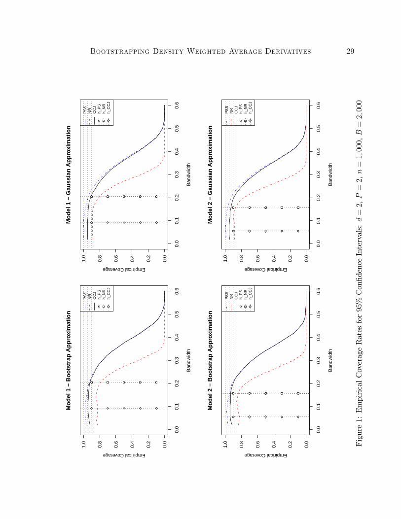
The results are summarized in Figure 1 (P = 2) and Figure 2 (P = 4). These figures

plot the empirical coverage for the three competing 95% confidence intervals as a function

of the choice of bandwidth. To facilitate the analysis two additional horizontal lines at 0.90

and at the nominal coverage rate 0.95 are included for reference. In each figure, the first

and second rows correspond to Models 1 and 2, respectively. Also, for each figure, the first

column depicts the results for the competing confidence intervals using the standard non-

parametric bootstrap to approximate the quantiles of interest, while the second column does

the same but using the large sample distribution quantiles (e.g., Φ−11 (0.975) ≈ 1.96). Finally,

each plot also includes three population bandwidth selectors available in the literature for

density-weighted average derivatives as vertical lines. Specifically, hPS, hNR and hCCJ de-

note the population “optimal”bandwidth choices described in Powell and Stoker (1996), NR

and Cattaneo, Crump, and Jansson (2010), respectively. The bandwidths differ in general,

although hPS = hNR when d = 2 and P = 2. (For a detailed discussion and comparison of

these bandwidth selectors, see Cattaneo, Crump, and Jansson (2010).)

The main results are consistent across all designs considered. First, it is seen that boot-

strapping PSS induces a “bias” in the distributional approximation for small bandwidths,


as predicted in Theorem 1. Second, bootstrapping CCJ (which uses V1,n) provides a close-

to-correct approximation for a range of small bandwidth choices, as predicted by Theorem

2. Third, by comparing these results across columns (bootstrapping vs. Gaussian approx-

imations), it is seen that the “bias” in the distributional approximation of PSS for small

bandwidths is smaller (leading to shorter confidence intervals) than the corresponding “bias”

introduced from using the Gaussian approximation (longer confidence intervals), as predicted

by Theorem 1.

In addition, it is found that the range of bandwidths with close-to-correct coverage has

been enlarged for both PSS and CCJ when using the bootstrap approximation instead of

the Gaussian approximation. The bias correction proposed by Nishiyama and Robinson

(2000, 2005) does not seem to work well when P = 2 (Figure 1), but works somewhat better

when P = 4 (Figure 2).7

Based on the theoretical results developed in this paper, and the simulation evidence

presented, it appears that confidence intervals based on the bootstrap distribution of CCJ

perform the best, as they are valid under quite weak conditions. In terms of bandwidth

selection, the Monte Carlo experiment shows that hCCJ falls clearly inside the “robust”

range of bandwidths in all cases. Interestingly, and because bootstrapping CCJ seems to

enlarge the “robust”range of bandwidths, the bandwidth selectors hPS and hNR also appear

to be “valid”when coupled with the bootstrapped confidence intervals based on CCJ∗.

5. Conclusion

Employing the “small bandwidth”asymptotic framework of CCJ, this paper has developed

theory-based predictions of finite sample behavior of a variety of bootstrap-based inference

procedures associated with the kernel-based density-weighted averaged derivative estimator

proposed by PSS. In important respects, the predictions and methodological prescriptions

emerging from the analysis presented here differ from those obtained using Edgeworth expan-

sions by NR. The results of a small-scale Monte Carlo experiment were found to be consistent

with the theory developed here, indicating in particular that while the properties of inference

procedures employing the variance estimator of PSS are very sensitive to bandwidth choice,

this sensitivity can be ameliorated by using a “robust”variance estimator proposed in CCJ.

7It seems plausible that these conclusions are sensitive to the choice of initial bandwidth bn for theconstruction of the estimator Bn, but we have made no attempt to improve on the initial bandwidth choiceadvocated by Nishiyama and Robinson (2000, 2005).


6. Appendix

For any λ ∈ Rd, let Uij,n (λ) = λ′[U (zi, zj;hn)− θ (hn)] and define the n-varying U -statistics

T1,n(λ) =

(n

2

)−1 ∑1≤i<j≤n

Uij,n(λ), T2,n(λ) =

(n

2

)−1 ∑1≤i<j≤n

Uij,n(λ)2,

T3,n(λ) =

(n

3

)−1 ∑1≤i<j<k≤n

Uij,n(λ)Uik,n(λ) + Uij,n(λ)Ujk,n(λ) + Uik,n(λ)Ujk,n(λ)

3,

T4,n(λ) =

(n

4

)−1 ∑1≤i<j<k<l≤n

Uij,n(λ)Ukl,n(λ) + Uik,n(λ)Ujl,n(λ) + Uil,n(λ)Ujk,n(λ)

3,

as well as their bootstrap analogues

T ∗1,m(λ) =

(m

2

)−1 ∑1≤i<j≤m

U∗ij,m(λ), T ∗2,m(λ) =

(m

2

)−1 ∑1≤i<j≤m

U∗ij,m(λ)2,

T ∗3,m(λ) =

(m

3

)−1 ∑1≤i<j<k≤m

U∗ij,m(λ)U∗ik,m(λ) + U∗ij,m(λ)U∗jk,m(λ) + U∗ik,m(λ)U∗jk,m(λ)

3,

T ∗4,m(λ) =

(m

4

)−1 ∑1≤i<j<k<l≤m

U∗ij,m(λ)U∗kl,m(λ) + U∗ik,m(λ)U∗jl,m(λ) + U∗il,m(λ)U∗jk,m(λ)

3,

where U∗ij,m(λ) = λ′[U(z∗i , z∗j ;hm) − θ∗ (hm)]. (Here, and elsewhere in the Appendix, the

dependence of m(n) on n has been suppressed.)

The proof of Lemma 2 uses four technical lemmas, proofs of which are available upon

request. The first lemma is a simple algebraic result relating Σn and ∆n (and their bootstrap

analogues) to T1,n, T2,n, T3,n, and T4,n (and their bootstrap analogues).

Lemma A-1. If the assumptions of Lemma 2 hold and if λ ∈ Rd, then

(a) λ′Σn(hn)λ = 4 [1 + o (1)]n−1T2,n(λ) + 4[1 + o (1)]T3,n(λ)− 4T1,n(λ)2,

(b) h−(d+2)n λ′∆n(hn)λ = [1 + o (1)]T2,n(λ)−T1,n(λ)2− 2[1 + o (1)]T3,n(λ) + 2[1 + o (1)]T4,n(λ),

(c) λ′Σ∗m(hm)λ = 4 [1 + o (1)]m−1T ∗2,m(λ) + 4[1 + o (1)]T ∗3,m(λ)− 4T ∗1,m(λ)2,

(d) h−(d+2)m λ′∆∗m(hm)λ = [1+o (1)]T ∗2,m(λ)−T ∗1,m(λ)2−2[1+o (1)]T ∗3,m(λ)+2[1+o (1)]T ∗4,m(λ).

The next lemma, which follows by standard properties of (n-varying) U -statistics (e.g.,

NR and CCJ), gives some asymptotic properties of T1,n, T2,n, T3,n, and T4,n (and their boot-


strap analogues). Let ηn = 1/min(1, nhd+2

n

).


(a) T1,n(λ) = op(√ηn),

(b) T2,n(λ) = E[Uij,n(λ)2] + op(h−(d+2)n ),

(c) T3,n(λ) = E[(E[Uij,n(λ)|zi])2] + op(ηn),

(d) T4,n(λ) = op (ηn),

(e) hd+2n E[Uij,n(λ)2]→ λ′∆λ and E[(E[Uij,n(λ)|zi])2]→ λ′Σλ/4,

(f) T ∗1,m(λ) = op(√ηm),

(g) T ∗2,m(λ) = E∗[U∗ij,m(λ)2] + op(h−(d+2)m ),

(h) T ∗3,m(λ) = E∗[(E[U∗ij,m(λ)|Zn, z∗i ])2] + op(ηm),

(i) T ∗4,m(λ) = op(ηm),

(j) hd+2m E∗[U∗ij,m(λ)2]→p λ

′∆λ and E∗[(E[U∗ij,m (λ) |Zn, z∗i ])2]− λ′Σn(hm)λ/4→p 0.

The next lemma, which can be established by expanding sums and using simple bounding

arguments, is used to establish a pointwise version of (4).


(a) E[(E[U∗ij,m(λ)|Zn, z∗i ])4] = O(η2m + h2

mη3m),

(b) E[U∗ij,m(λ)4] = O(h−(3d+4)m ),

(c) E[(E[U∗ij,m(λ)2|Zn, z∗i ])2] = O(m−1h−(3d+4)m + h

−(2d+4)m ),

(d) E[(E[U∗ij,m(λ)U∗ik,m(λ)|Zn, z∗j , z∗k])2] = O(h−(d+4)m +m−2h

−(3d+4)m ),

(e) E[(E[E[U∗ij,m(λ)|Zn, z∗i ]U∗ij,m(λ)|Zn, z∗j ])2] = O(1 +m−1h−(d+4)m +m−3h

−(3d+4)m ).

Finally, the following lemma about quadratic forms is used to deduce (4) from its point-

wise counterpart.

Lemma A-4. There exist constants C and J (only dependent on d) and a collection

l1, . . . , lJ ∈ Λd such that, for every d× d matrix M ,

supλ∈Λd

(λ′Mλ)2 ≤ C

J∑j=1

(l′jMlj

)2.

Proof of Lemma 2. By the properties of the (conditional on Zn) Hoeffding decompo-


sition, E[L∗(z∗i ;h)|Zn] = 0 and E[W ∗(z∗i , z∗j ;h)|Zn, z∗i ] = 0, so

V∗[θ∗m] = m−1V∗[L∗ (z∗i ;hm)] +

(m

2

)−1

V∗[W ∗(z∗i , z∗j ;hm)],

where, using Lemmas A-1 and A-2,

V∗[L∗(z∗i ;hm)] =

(n− 1

n

)2

Σn(hm) = Σ + 2m2

n

(m

2

)−1

h−(d+2)m ∆ + op (ηm) .

Also, for any λ ∈ Rd, it can be shown that

λ′V∗[W ∗(z∗i , z∗j ;hm)]λ = h−(d+2)

m

(n− 1

n

)[λ′∆n(hm)λ+ op (1)

]− 3

2

(n− 1

n

)2

λ′Σn(hm)λ.

Therefore, using Lemmas A-1 and A-2,

V∗[W ∗(z∗i , z∗j ;hm)] = h−(d+2)

m ∆ + op (mηm) ,

completing the proof of part (a).

Next, using Lemmas A-1 and A-2,

λ′Σ∗m(hm)λ = 4[1 + o (1)]m−1T ∗2,m(λ) + 4[1 + o (1)]T ∗3,m(λ)− 4T ∗1,m(λ)2

= λ′Σn(hm)λ+ 4m−1h−(d+2)m λ′∆λ+ op(ηm)

= λ′Σ∗mλ+ op (ηm) ,

establishing part (b).

Finally, to establish part (c), the theorem of Heyde and Brown (1970) is employed to

prove the following condition, which is equivalent to (4) in view of part (a):

supλ∈Λd

supt∈Rd

∣∣∣∣∣∣P∗λ′(θ∗m − θ∗m)√

λ′V∗[θ∗m]λ

≤ t

− Φ1 (t)

∣∣∣∣∣∣→p 0.

For any λ ∈ Λd,λ′θ∗m − λ′θ∗m√λ′V∗[θ

∗m]λ

=

m∑i=1

Y ∗i,m (λ) ,


where, defining L∗i,m (λ) = λ′L∗(z∗i ;hm) and W ∗ij,m (λ) = λ′W ∗(z∗j , z

∗i ;hm),

Y ∗i,m (λ) =1√

λ′V∗[θ∗m]λ

[m−1L∗i,m (λ) +

i−1∑j=1

(m

2

)−1

W ∗ij,m (λ)

].

For any n,(Y ∗i,m (λ) ,F∗i,n

)is a martingale difference sequence, whereF∗i,n = σ (Zn, z∗1 , . . . , z∗i ) .

Therefore, by the theorem of Heyde and Brown (1970), there exists a constant C such that

supλ∈Λd

supt∈Rd

∣∣∣∣∣∣P∗λ′(θ∗m − θ∗m)√

λ′V∗[θ∗m]λ

≤ t

− Φ1 (t)

∣∣∣∣∣∣≤ C sup

λ∈Λd

m∑i=1

E∗[Y ∗i,m (λ)4]+ E∗

( m∑i=1

E[Y ∗i,m (λ)2

∣∣F∗i−1,n

]− 1

)2

1/5

.

Moreover, by Lemma A-4,

supλ∈Λd

m∑i=1

E∗[Y ∗i,m (λ)4]+ E∗

( m∑i=1

E[Y ∗i,m (λ)2

∣∣F∗i−1,n

]− 1

)2→p 0

if (and only if) the following hold for every λ ∈ Λd:

m∑i=1

E∗[Y ∗i,m (λ)4]→p 0 (5)

and

E∗( m∑

i=1

E[Y ∗i,m (λ)2

∣∣F∗i−1,n

]− 1

)2→p 0. (6)

The proof of part (c) will be completed by fixing λ ∈ Λd and verifying (5)—(6) . First,

using (λ′V∗[θ∗m]λ)−1 = Op(mη

−1m ) and basic inequalities, it can be shown that (5) holds if

R1,m = m−2η−2m

m∑i=1

E[L∗i,m (λ)4]→ 0


and

R2,m = m−6η−2m

m∑i=1

E

( i−1∑j=1

W ∗ij,m (λ)

)4→ 0.

Both conditions are satisfied because, using Lemma A-3,

R1,m = O(m−1η−2

m E[(E[U∗ij,m (λ) |Zn, z∗i ])4])

= O(m−1 +m−1h2

mηm)

= O(m−1 +m−2h−dm

)→ 0

and

R2,m = O(m−4η−2

m E[U∗ij,m (λ)4

]+m−3η−2

m E[(E[U∗ij,m (λ)2 |Zn, z∗i ])2])

= O(m−4η−2

m h−(3d+4)m +m−3η−2

m h−(2d+4)m

)= O

(m−2h−dm +m−1

)→ 0.

Next, consider (6). Because

(λ′V∗[θ∗m]λ)

[m∑i=1

E[Y ∗i,m (λ)2

∣∣F∗i−1,n

]− 1

]

=

(m

2

)−2 m∑i=1

E( i−1∑

j=1

W ∗ij,m (λ)

)2∣∣∣∣∣∣F∗i−1,n

− i−1∑j=1

E∗[W ∗ij,m (λ)2]

+ 2m−1

(m

2

)−1 m∑i=1

i−1∑j=1

E[L∗i,m (λ)W ∗

ij,m (λ) |F∗i−1,n

],

it suffi ces to show that

R3,m = m−6η−2m E

( m∑i=1

i−1∑j=1

E[W ∗ij,m (λ)2

∣∣F∗i−1,n

]− E∗

[W ∗ij,m (λ)2])2

→ 0,

R4,m = m−6η−2m E

( m∑i=1

i−1∑j=1

j−1∑k=1

E[W ∗ij,m (λ)W ∗

ik,m (λ)∣∣F∗i−1,n

])2→ 0,

R5,m = m−4η−2m E

( m∑i=1

i−1∑j=1

E[L∗i,m (λ)W ∗

ij,m (λ) |Zn, z∗j])2

→ 0.


By simple calculations and Lemma A-3,

R3,m = O(m−4η−2

m E[W ∗ij,m (λ)4]

)= O

(m−4η−2

m E[U∗ij,m (λ)4])

= O(m−4η−2

m h−(3d+4)m

)= O

(m−2h−dm

)→ 0,

R4,m = O(m−2η−2

m E[(E[W ∗

ij,m (λ)W ∗ik,m (λ) |Zn, z∗j , z∗k]

)2])

= O

(m−2η−2

m E[(E[U∗ij,m (λ) U∗ik,m (λ) |Zn, z∗j , z∗k]

)2])

= O(m−2η−2

m h−(d+4)m +m−4η−2

m h−(3d+4)m

)= O

(hdm +m−2h−dm

)→ 0,

R5,m = O(m−1η−2

m E[(E[L∗i,m (λ)W ∗

ij,m (λ) |Zn, z∗j])2])

= O

(m−1η−2

m E[(E[E[U∗ij,m (λ) |Zn, z∗i ]U∗ij,m (λ) |Zn, z∗j

])2])

= O(m−1η−2

m +m−2η−2m h−(d+4)

m +m−4η−2m h−(3d+4)

m

)= O

(m−1 + hdm +m−2hdm

)→ 0,

as was to be shown.


ReferencesAbadie, A., and G. W. Imbens (2008): “On the Failure of the Bootstrap for MatchingEstimators,”Econometrica, 76(6), 1537—1557.

Andrews, D. W. K., and M. Buchinsky (2000): “A Three-Step Method for Choosingthe Number of Bootstrap Repetitions,”Econometrica, 68(1), 23—51.

Cattaneo, M. D., R. K. Crump, and M. Jansson (2009): “Small Bandwidth Asymp-totics for Density-Weighted Average Derivatives,”working paper.

(2010): “Robust Data-Driven Inference for Density-Weighted Average Derivatives,”forthcoming in Journal of the American Statistical Association.

Chen, X. (2007): “Large Sample Sieve Estimation of Semi-Nonparametric Models,” inHandbook of Econometrics, Volume VI, ed. by J. J. Heckman, and E. Leamer, pp. 5549—5632. Elsevier Science B.V., New York.

Chen, X., O. Linton, and van Keilegom (2003): “Estimation of Semiparametric Modelswhen The Criterion Function Is Not Smooth,”Econometrica, 71(5), 1591—1608.

Gine, E., and J. Zinn (1990): “Bootstrapping General Empirical Measures,”Annals ofProbability, 18(2), 851—869.

Gonçalves, S., and T. J. Vogelsang (2010): “Block Bootstrap HAC Robust Tests: TheSophistication of the Naive Bootstrap,”forthcoming in Econometric Theory.

Heyde, C. C., and B. M. Brown (1970): “On the Departure from Normality of a CertainClass of Martingales,”Annals of Mathematical Statistics, 41(6), 2161—2165.

Horowitz, J. (2001): “The Bootstrap,” in Handbook of Econometrics, Volume V, ed. byJ. Heckman, and E. Leamer, pp. 3159—3228. Elsevier Science B.V., New York.

Kiefer, N. M., and T. J. Vogelsang (2005): “A New Asymptotic Theory forHeteroskedasticity-Autocorrelation Robust Tests,” Econometric Theory, 21(6), 1130—1164.

Linton, O. (1995): “Second Order Approximation in the Partialy Linear RegressionModel,”Econometrica, 63(5), 1079—1112.

Newey, W. K. (1994a): “The Asymptotic Variance of Semiparametric Estimators,”Econo-metrica, 62(6), 1349—1382.

(1994b): “Kernel Estimation of Partial Means and a General Variance Estimator,”Econometric Theory, 10(2), 1349—1382.


Newey, W. K., and D. L. McFadden (1994): “Large Sample Estimation and Hypoth-esis Testing,” in Handbook of Econometrics, Volume IV, ed. by R. F. Engle, and D. L.McFadden, pp. 2111—2245. Elsevier Science B.V., New York.

Nishiyama, Y., and P. M. Robinson (2000): “Edgeworth Expansions for SemiparametricAveraged Derivatives,”Econometrica, 68(4), 931—979.

(2001): “Studentization in Edgeworth Expansions for Estimates of SemiparametricIndex Models,”in Nonlinear Statistical Modeling: Essays in Honor of Takeshi Amemiya,ed. by C. Hsiao, K. Morimune, and J. L. Powell, pp. 197—240. Cambridge University Press,New York.

(2005): “The Bootstrap and the Edgeworth Correction for Semiparametric AveragedDerivatives,”Econometrica, 73(3), 197—240.

Politis, D., J. Romano, and M. Wolf (1999): Subsampling. Springer, New York.

Powell, J. L., J. H. Stock, and T. M. Stoker (1989): “Semiparametric Estimation ofIndex Coeffi cients,”Econometrica, 57(6), 1403—1430.

Powell, J. L., and T. M. Stoker (1996): “Optimal Bandwidth Choice for Density-Weighted Averages,”Journal of Econometrics, 75(2), 291—316.

Xiong, S., and G. Li (2008): “Some Results on the Convergence of Conditional Distribu-tions,”Statistics and Probability Letters, 78(18), 3249—3253.


Table1:SummaryofMainResults

limn→∞nhd+

2n

=κ∈R

+limn→∞nhd+

2n6=

limn→∞nhd+

2n

κ=∞

κ∈

(0,∞

)κ

=0

PSS

Largesampledistribution

N(0,Id)

N(0,Ω

0)

N(0,Id/2

)—

Standardbootstrap

N(0,Id)

N(0,Ω∗ 0)

N(0,3I d/4

)—

Replacementsubsampling

N(0,Id)

N(0,Ω

0)

N(0,Id/2

)—

CCJ 1


N(0,Id)

N(0,Id)

N(0,Id)

N(0,Id)

Standardbootstrap

N(0,Id)

N(0,Id)

N(0,Id)

N(0,Id)


N(0,Id)

N(0,Id)

N(0,Id)

N(0,Id)

CCJ 2


N(0,Id)

N(0,Id)

N(0,Id)

N(0,Id)

Standardbootstrap

N(0,Id)

N(0,Ω∗ 2)

N(0,3I d/2

)—


N(0,Id)

N(0,Id)

N(0,Id)

N(0,Id)

Notes:

(i)PSS,CCJ 1andCCJ 2denotethestudentizedteststatisticsusingV0,n,V1,nandV2,n,respectively.

(ii)

Ω0,

Ω∗ 0,

Ω∗ 2aredefinedinLemma1(b),Theorem

1(b)andTheorem

3(a),respectively.

(iii)Lemmas1—2specifyotherassumptionsandconditionsimposed.


0.0

0.1

0.2

0.3

0.4

0.5

0.6

0.0

0.2

0.4

0.6

0.8

1.0

Mo

del

1 −

Bo

ots

trap

Ap

pro

xim

atio

n

Ban

dwid

th

Empirical Coverage

PS

SN

RC

CJ

h_P

Sh_

NR

h_C

CJ

0.0

0.1

0.2

0.3

0.4

0.5

0.6

0.0

0.2

0.4

0.6

0.8

1.0

Mo

del

1 −

Gau

ssia

n A

pp

roxi

mat

ion

Ban

dwid

th

Empirical Coverage

PS

SN

RC

CJ

h_P

Sh_

NR

h_C

CJ

0.0

0.1

0.2

0.3

0.4

0.5

0.6

0.0

0.2

0.4

0.6

0.8

1.0

Mo

del

2 −

Bo

ots

trap

Ap

pro

xim

atio

n

Ban

dwid

th

Empirical Coverage

PS

SN

RC

CJ

h_P

Sh_

NR

h_C

CJ

0.0

0.1

0.2

0.3

0.4

0.5

0.6

0.0

0.2

0.4

0.6

0.8

1.0

Mo

del

2 −

Gau

ssia

n A

pp

roxi

mat

ion

Ban

dwid

th

Empirical Coverage

PS

SN

RC

CJ

h_P

Sh_

NR

h_C

CJ

Figure1:EmpiricalCoverageRatesfor95%ConfidenceIntervals:d

=2,P

=2,n

=1,

000,B

=2,

000


0.0

0.2

0.4

0.6

0.8

0.0

0.2

0.4

0.6

0.8

1.0

Mo

del

1 −

Bo

ots

trap

Ap

pro

xim

atio

n

Ban

dwid

th

Empirical Coverage

PS

SN

RC

CJ

h_P

Sh_

NR

h_C

CJ

0.0

0.2

0.4

0.6

0.8

0.0

0.2

0.4

0.6

0.8

1.0

Mo

del

1 −

Gau

ssia

n A

pp

roxi

mat

ion

Ban

dwid

th

Empirical Coverage

PS

SN

RC

CJ

h_P

Sh_

NR

h_C

CJ

0.0

0.2

0.4

0.6

0.8

0.0

0.2

0.4

0.6

0.8

1.0

Mo

del

2 −

Bo

ots

trap

Ap

pro

xim

atio

n

Ban

dwid

th

Empirical Coverage

PS

SN

RC

CJ

h_P

Sh_

NR

h_C

CJ

0.0

0.2

0.4

0.6

0.8

0.0

0.2

0.4

0.6

0.8

1.0

Mo

del

2 −

Gau

ssia

n A

pp

roxi

mat

ion

Ban

dwid

th

Empirical Coverage

PS

SN

RC

CJ

h_P

Sh_

NR

h_C

CJ

Figure2:EmpiricalCoverageRatesfor95%ConfidenceIntervals:d

=2,P

=4,n

=1,

000,B

=2,

000

Many Terms in a Series Estimator of the Partially Linear Model1

Matias D. Cattaneo, Department of Economics, University of Michigan, [email protected].

Michael Jansson, Department of Economics, UC Berkeley, [email protected].

Whitney K. Newey, Department of Economics, MIT, [email protected].

September, 2010

VERY PRELIMINARY AND INCOMPLETE DRAFT

JEL classication: C13, C31.

Keywords: partially linear model, many terms, adjusted variance.

1This very preliminary version of the paper was prepared for the Fourth Annual Meeting of the Impact EvaluationNetwork (IEN), Latin American and the Caribbean Economic Association (LACEA).

mailto:[email protected]



Proposed Running Head: Many Terms Asymptotics

Corresponding Author:

Whitney K. Newey

Department of Economics

MIT, E52-262D

Cambridge, MA 02142-1347

Abstract

This papers studies the asymptotic behavior of a series-based semiparametric estimator for the

partially linear model, and derives a generalized large sample theory that accommodates (but does

not require) a large number of terms (or covariates) relative to the sample size. This asymp-

totic distribution theory covers the classical large sample results based on the asymptotic linear

representation of the estimator, and also provides a distributional approximation even when the es-

timator is not asymptotically linear. Using these large sample results, it is shown that the classical

unbiased standard errors estimator from least squares theory is consistent under homoskedastic-

ity, even when the number of regressors grows proportionally to the sample size. On the other

hand, the classical Eicker-Huber-White heteroskedasticity-robust standard errors are shown to be

inconsistent in general. Two new heteroskedasticity- and many terms-robust standard errors are

proposed.

1

1 Introduction

Semiparametric procedures are popular in econometrics because they reduce misspecication biases

while retaining many of the attractive properties of parametric modelling. These procedures typi-

cally require choosing a preliminary nonparametric estimator that depends on user-dened tuning

and smoothing parameters (e.g., a bandwidth and a kernel, or the number of terms in and a form

of series of approximation). Unfortunately, such procedures are considerably less popular among

empirical researchers because inference based on classical large sample approximations is known

to be highly sensitive to perturbations in the choice of tuning and smoothing parameters, making

empirical work unreliable in general. The lack of robustness of semiparametric-based statistical

procedures with respect to changes in these parameters is a common problem in many econometric

models. As a consequence, inference procedures that are insensitive to changes in the tuning and

smoothing parameters are highly desirable, as they will increase substantially the validity of the

empirical results obtained in specic empirical applications.

This papers studies the asymptotic behavior of a series-based semiparametric estimator for the

partially linear model, and derives a generalized large sample theory based on an alternative as-

ymptotic experiment. Specically, this paper studies the asymptotic behavior of the corresponding

semiparametric t-test under tuning parameter sequences (i.e., the number of terms in the series

approximation) that may render asymptotic linearity invalid, and hence capturing features of the

semiparametric statistic that are typically assumed away by conventional large sample results (e.g.,

Newey and McFadden (1994) and Chen (2007)). This type of large sample approximations have

been shown to provide a better nite sample characterization of the statistic of interest, when

compared to the classical, asymptotically linear distributional approximations. This idea has been

employed in a variety of contexts, including matching estimators with xed number of matches

(Abadie and Imbens (2006)), IV estimators with many/weak instruments (Hansen, Hausman, and

Newey (2008)), and density-weigthed average derivatives (Cattaneo, Crump, and Jansson (2010)).

The new asymptotic approximation presented here is not only important from a theoretical

point of view, but also relevant for applications. The semiparametric linear model is popular among

empirical researchers because ts naturally into a control functionapproach, is a commonly used

dimension reduction technique, and may be justied in the context of a conditional independence

assumption. Moreover, as discussed in detail below, the theoretical results presented here also

apply to linear models where the number of regressors is large compared to the sample size, even

if there is no approximation bias.

This paper presents four main results. First, it is shown that a generalized central limit theorem

may be obtained for the classical series-based partially linear estimator, which is based on an ap-

proximate bilinear expansion. This result is shown to cover the classical asymptotic approximation

under conventional asymptotics, although in general the estimator has a larger asymptotic variance,

2

which is not invariant with respect to the tuning and smoothing parameters employed. Second, it

is shown that under known homoskedasticity the classical degrees-of-freedom-corrected standard

errors estimator from least squares is valid, even when the number of terms in the approximation

series is large. Third, it is shown that the conventional Eicker-Huber-White heteroskedasticity-

robust (HR) standard errors estimator is inconsistent in general under the generalized asymptotics.

In particular, when the underlying model is homoskedastic, the HR standard errors estimator is

biased downwards, leading to liberal inference. Finally, three new HR standard errors estimators

are proposed that are also asymptotically valid when the number of terms (or regressors) is large

relative to the sample size.

2 Model and Classical Results

Let (yi; x0i; z0i)0, i = 1; : : : ; n, be a random sample of the random vector (y; x0; z0)0, where y 2 R

is a dependent variable, and x 2 Rdx1 and z 2 Rdz1 are explanatory variables. The so-calledpartially linear model is given by

yi = x0i + g(zi) + "i, E ["ijxi; zi] = 0, 2(xi; zi) = E"2i jxi; zi

,

where vi = xi h(zi), with h(zi) = E [xijzi].2 Donald and Newey (1994) provide su¢ cient

conditions forpn-consistency and asymptotic linearity of a series-based semiparametric estima-

tor of . Specically, the estimator is constructed by regressing yi on xi and pK(zi), where

pK(z) = (pK1(z); : : : ; pKK(z))0 is an appropriate basis of approximation, such as polynomials or

splines, and K = K (n)!1.To formally describe this estimator, let Y = [y1; ; yn]0 2 Rn1, X = [x1; ; xn]0 2 Rndx ,

Z = [z1; ; zn]0 2 Rndz , " = ["1; ; "n]0 2 Rn1, V = [v1; ; vn]0 2 Rndx , G = [g(z1); ; g(zn)]0 2Rn1, H = [h(z1); ; h(zn)]0 2 Rndx , and P = [pK(z1); : : : ; pK(zn)]0. The series-based estimatorof is given by

= (X 0MX)X 0MY , M = I Q, Q = P (P 0P )P 0,

where A denotes a generalized inverse of a matrix A (satisfying AAA = A). For xed n,

this estimator coincides with a partial-out regression estimator = ( ~X 0 ~X) ~X 0 ~Y , where ~X =

MX = [~x1; ; ~xn]0 and ~Y = MY = [~y1; ; ~yn]0. (Similarly, denote ~" = M" = [~"1; ;~"n]0 and~V =MV = [~v1; ; ~vn]0.)The estimator may be intuitively interpreted as a two-step semiparametric estimator with

smoothing parameter pK () and tuning parameter K, because the unknown (regression) functions2See Robinson (1988) for the analysis of this model when using kernel regression, and Linton (1995) for the

corresponding higher-order properties.

3

g() and h () are non-parametrically estimated in a preliminary step by the series estimator. Inparticular, the following assumption characterizes the rate at which the approximation error of

series estimator should vanish.

Assumption B. (i) For some h > 0, there exists h so that

1

nH 0MH =

1

nminkH Pk2 = 1

n

nXi=1

h (zi) pK (zi)0 h 2 = Oas(K2h).

(ii) For some g > 0, there exists g so that

1

nG0MG =

1

nminkG Pk2 = 1

n

nXi=1

g (zi) pK (zi)0 g

2= Oas(K

2g).

The conditions required in Assumption B are implied by conventional assumptions from the

series-based nonparametric literature (e.g., Newey (1997, Assumption 3)). Thus, under appropriate

assumptions, commonly used basis of approximation such as polynomials or splines will satisfy

Assumption B with h = dz=sh and g = dz=sg, where sh and sg denotes the number of continuous

derivatives of h and g, respectively.

Under regularity conditions (given in Section 3) and Assumption B, Donald and Newey (1994)

obtained the following (infeasible) classical asymptotic approximation for : if

nK2(h+g) ! 0 andK

n! 0 (1)

thenpn( ) = 1p

n

nXi=1

i + op(1)!d N (0;) , = 11, (2)

where

i = 1vi"i, = E

viv

0i

, = E

viV ["jX;Z] v0i

.

The classical asymptotic linear representation of , given in (2), is established by analyzing the

rst-order stochastic properties of the numeratorand denominatorof the estimator. Intuitively,

in each case, the analysis proceeds by rst nding conditions so thatQX H andQ (Y X) G,

which captures the bias introduced by the series approximation, and then nding conditions so that

the corresponding reminders are well-behaved asymptotically. Specically, for the denominator

of , it can be shown (see Lemma 1 below) that if Condition (1) holds, then the (Hessian) matrix

4

satises (recall that M = I Q and QP = P )

n =1

nX 0MX 1

nV 0MV =

1

nV 0V 1

nV 0QV 1

n

nXi=1

viv0i !p ,

where the rst approximation captures the bias introduced by the series estimator (Assumption

B(i)), and the second approximation requires the contribution of V 0QV to vanish asymptotically.

Similarly, for the numeratorof , it can be shown (see Lemmas 24 below) that

1pnX 0M (Y X) 1p

nV 0M" =

1pnV 0" 1p

nV 0Q" 1p

n

nXi=1

vi"i !d N (0;) ,

where the rst approximation is again related to the bias introduced by the nonparametric estimator

and the second approximation requires V 0Q" to be asymptotically negligible.

In both cases, the approximation error associated with the bias is controlled by the condition

nK2(h+g) ! 0, which requires K to be large(provided the underlying functions g and h are

smooth enough). On the other hand, condition K=n ! 0 guarantees that both V 0QV and V 0Q"

are asymptotically negligible, as required for the classical, asymptotically linear, approximation to

be valid. The latter condition controls the variance of the estimator, and it is directly related to

the behavior of the nonparametric estimator, which in this case is described by Q.

The classical approach to form a condence interval for 0 is to use the asymptotic distribu-

tional result coupled with a consistent standard errors estimator. A plug-in approach employs the

(asymptotically) pivotal test statistic T0;n(K) = 1=20

pn(), together with a plug-in consistent

estimator for 0. Under heteroskedasticity, the feasible test statistic is given by

T0;n(Kn) = 1=2n

pn( ), n =

1n n

1n ,

where

n =X 0MX

n, n =

1

nK dx

nXi=1

~xi~x0i"2i , " = ~Y ~X 0 = ["1; ; "n]0.

In this case, the standard errors estimator is the classical Heteroskedasticity-Robust (HR) stan-

dard errors estimator commonly used in regression analysis. Under Condition (1) it is not di¢ cult

to show that 1n 0 !p Idx .

3 Generalized Asymptotic Distribution

This section derives a generalized asymptotic distribution forpn(), which relaxes the condition

Kn=n! 0. This non-standard asymptotic theory encompasses the classical result discussed in the

5

previous section, and also captures the e¤ect of the quadratic term of the expansion, which is

assumed away by Condition (1). Intuitively, this asymptotic experiment captures the e¤ect of K

large(relative to n) by breaking down the asymptotic linearity of the estimator.

To characterize the generalized central limit theory, it is natural to study the stochastic behavior

of the estimatorpn( ) as a ratioof two bilinear forms:

pn( ) =

1

nX 0MX

1pnX 0M (Y X) = n

1pnX 0M (Y X) .

The following lemma characterizes the behavior of the Hessian matrix n under quite weak

conditions. (Throughout this paper Aij denotes the (i; j)-th element of a matrix A.)

Lemma 1. Suppose that E[kvik4 jzi] Cv <1 (a.s.) and Assumption B(i) holds. Then,

n =1

nX 0MX = n + op(K=n), n =

1

n

nXi=1

MiiEviv

0ijzi= Oas(1 +K=n).

This lemma characterizes the stochastic behavior of the Hessian matrix under conditions that

are weaker than those entertained by the classical, asymptotically linear, distribution theory. Specif-

ically, because M = IQ is an idempotent symmetric matrix, Mii 2 (0; 1) andPni=1Mii nK,

Lemma 1 implies that n remains asymptotically bounded even when K=n 6! 0. In particu-

lar, n = E [viv0i] + op (1) when K=n ! 0. Moreover, in the case of homoskedasticity of vi,

that is, if E [viv0ijzi] = E [viv0i] (and rank (Q) = K), then n = (1K=n)E [viv0i]. Finally, if

min (E [viv0ijzi]) FV > 0 and Mii = 1 Qii FQ > 0 (a.s.) then min (n) FQFV > 0.

(min (A) denotes the minimum eigenvalue of a matrix A.)

To fully characterize the asymptotic behavior of the numeratorofpn( ) it is convenient

to proceed in two steps. First, under appropriate bias assumptions, it is possible to show that the

numerator is asymptotically equivalent to quadratic form based on mean-zero random variables.

Lemma 2. Suppose the assumptions of Lemma 1 hold, and E["4i jzi] C" < 1 (a.s.) and

Assumption B(ii) holds. Then,

1pnX 0M (Y X) = 1p

nV 0M"+Op(

pnK(h+g) +Kh +Kg).

As in Lemma 1, this result only requires bounded moments and a bias condition. In this case,

the bias arises from both the approximation of the unknown functions h and g. As mentioned above,

6

the high-level Assumption B is implied by the standard assumption of best approximation from the

sieve literature. Interestingly, in this model there is a trade-o¤ in terms of curse of dimensionality:

provided that min fh; gg > 0, the bias condition is given bypnK(h+g) ! 0, which implies a

trade-o¤ between smoothness and dimensionality between h and g.

Lemma 2 justies focusing on the bilinear form

n =1pnV 0M" =

1pn

nXi=1

nXj=1

Mijvi"j ,

where E [njZ;X] = 0. Moreover, under the assumptions imposed in Lemma 2, a simple variancecalculation yields

n = V [njZ] =1

n

nXi=1

nXj=1

M2ijE[viv0i"2j jzi; zj ] = Oas

1 +

K

n

.

In particular, if K=n! 0 then

n =1

n

nXi=1

M2iiEviv

0i"2i jzi+ op (1) = E

viv

0i"2i

+ op (1) = + op (1) ,

as given in Section 2. Moreover, under homoskedasticity, that is, if E"2i jxi; zi

= 2, then

V1pnV 0M"

X;Z = 2

nV 0MV ,

and

n =2

n

nXi=1

nXj=1

M2ijEviv

0ijzi= 2n,

becausePnj=1M

2ij =Mii. Furthermore, if E

"2i jxi; zi

= 2 and E [viv0ijzi] = E [viv0i] (and rank (Q) =

K (a.s.)), then n = 2 (1K=n)E [viv0i]. Finally, if minEviv

0i"2jzi FV " > 0 and Mii =

1Qii FQ > 0 (a.s.), then min (n) F 2QFV " > 0.

The following Lemma characterizes the asymptotic distribution of the bilinear form n.

Lemma 3. Suppose the assumptions of Lemma 2 hold, and Mii > FM > 0 (a.s.) and

min (n) > F > 0 (a.s.). Then,

1=2n

1pnV 0M"!d N (0; Idx) .

The following theorem is a direct consequence of the previous lemmas and Slutsky Theorem,

7

and constitutes the main result of this section.

Theorem 1. Suppose the assumptions Lemma 3 hold and suppose min (n) > FH > 0. Then,

if

nK2(x+g) ! 0 andK

n! 2 [0; 1) (3)

then

1=2n ( )!d N (0; Idx) . (4)

If, moreover, (n;n) = (1;1) + op (1) for some (1;1), then

pn( )!d N (0;1) , 1 = 11 1

11 .

If, moreover, E"2i jxi; zi

= 2 for some 2, then

pn( )!d N

0; 211

.

Theorem 1 shows that the central limit theorem for holds under the weaker condition (3).

(Compare to Condition (1).) This result does not rely on asymptotic linearity, nor on the actual

convergence of the matrices n and n. However, if K=n! 0, then (n;n) = (;)+ op (1) with

= E [viv0i] and = Eviv

0i"2i

, and the resulting large sample distribution theory does rely on the

asymptotically linear representation of , as given in (2).

Importantly, if K=n 9 0 and (n;n) = (;) + op (1), then 6= E [viv0i] and 6= Eviv

0i"2i

,

in general. For instance, if (vi; "i) is independent of zi, then n = (1K=n)E [viv0i] and

n =

1 K

n

Eviv

0i"2i

+

1

n

nXi=1

Q2ii K

n

!Eviv

0i"2i

E

viv

0i

E"2i.

4 Standard Errors

This section discusses di¤erent homoskedastic- and heteroskedastic- standard errors estimators, and

their properties under the generalized asymptotics studied in this paper.

4.1 Homoskedasticity

If E"2i jxi; zi

= 2 for all i = 1; 2; ; n, then n = 2n . Thus, a natural plug-in estimator is

given by VHOM = 2, where 2 is chosen so that 2 = 2 + op (1). The usual OLS estimator is

2n =1

nK dx

nXi=1

"2i =1

nK dx"0".

8

As shown in Lemma 1, n = n + op(1) under the many terms asymptotics discussed in this

paper (Condition (3)), and therefore it remains to verify that 2n is also consistent under this

generalized asymptotic experiment. Heuristically, this estimator is consistent because

"0" = (Y X)0M(Y X) "0M" (nK)2,

where the rst approximation is based on thepn-consistency of and the approximation bias of

the series estimator, while the second approximation is based on the fact that the bilinear form

"0M" = "0(I Q)" is dominated by its diagonal. These heuristics are formalized in the following

theorem.

Theorem 2. Suppose the assumptions of Theorem 1 hold. Then, 2n = 2 + op (1).

It follows by Lemma 1, Theorem 2 and Slutsky Theorem that

VHOM = 2n + op (1) = n + op (1) ,

and therefore

V1=2HOM ( 0)!d N (0; Id) ,

under Condition (3). Thus, under known homoskedasticity, the usual nite sample standard errors

estimator from least squares theory turns out to be valid even when K is large. However, the con-

sistent but biased standard errors estimator ("0"=n)n will not be consistent unless K=n ! 0,

which implies that using the nite sample, unbiased standard errors estimator under homoskedas-

ticity is important even in large samples when the degrees of freedom is small (i.e., when K is

large).

4.2 Heteroskedasticity

Under heteroskedasticity of unknown form, a natural candidate for standard errors estimator is the

(family of) Eicker-Huber-White estimators given by

VHR = ( ~X0 ~X) ~X 0 ~X( ~X 0 ~X) =

1

nn n

n ,

n =1

nX 0MMX, = diag

!1"

21; ; !n"2n

=

2664!1"

21

. . .

!n"2n

3775where f!i : i = 1; ; ng are appropriate weights. Classical choices of weights include !i = 1,

!i = n=(nKdx), !i =M1ii , etc. Since n = n+op(1) according to Lemma 1, it only remains

9

to characterized the middle matrix of this classical sandwich formula. Heuristically, the asymptotic

properties of n are given by

n =1

n

nXi=1

!i~xi~x0i"2i

1

n

nXi=1

!i~vi~v0i~"2i

1

n

nXi=1

E!i~vi~v

0i~"2i

Z ,where, as before, the rst approximation captures the bias of the series estimator and removes

the estimation error of , and the second approximation shows that a (conditional) law of large

numbers holds in this case (i.e., a variance condition). This idea is summarized in the following

theorem.

Theorem 3. Suppose the assumptions of Theorem 1 hold with h > 1=2, and !i 2 (Z) forall i. Then, n = ~n + op(1), where

~n =1

n

nXi=1

nXj=1

nX`=1

!iM2i`M

2j`

!Eviv

0i"2j

zi; zj .

Recall that the population asymptotic middle matrix n is given by

n =1

n

nXi=1

nXj=1

M2ijE[viv0i"2j jzi; zj ],

which implies that the classical HR standard errors will not be consistent in general when Condition

(3). For example, the bias may be characterized under homoskedasticity: assuming E"2i jxi; zi

=

2 and !i = 1, a simple calculation yields

n =2

n

nXi=1

MiiEviv

0ijzi,

while, using basic properties of idempotent matrices, it is easy to verify that

~n = n 1

n

nXi=1

nXj=1

M2ij (1Mjj)E

viv

0ijzi< n.

As a consequence, the classical Eicker-Huber-White estimator is downward biased when K is

large. It is important to note that this result continue to hold in a simple linear model where

the number of regressors is largewhen compared to the sample size. Therefore, there is an im-

portant sense in which the classical HR standard errors estimator is not robust, even in a simple

linear model.

10

On the other hand, if K=n ! 0, then the asymptotic results presented above imply that~n = n+op(1), which veries that the classical HR standard errors estimator is indeed consistent

under heteroskedasticity of unknown form.

4.3 HR and Many Terms Robust Standard Errors

Intuitively, the failure of the classical HR standard errors estimator is due to the fact that both ~xiand "i are estimated with too much error when K=n 6! 0. Thus, it is possible to x this problem by

considering alternative (consistent) estimators for either ~xi or "i. To describe the new estimators,

let Kg and Kh be two choices of truncation for an approximation series, and let

~X = (I Qh)X, Qh = PKh(P 0Kh

PKh)P 0Kh

, Mh = I Qh,

" = (I Qg)", Qg = PKg(P0KgPKg)

P 0Kg, Mg = I Qg.

Using this notation, Theorem 3 may be extended to the following result.

Theorem 4. Suppose the assumptions of Theorem 3 hold, then

n =1

n

nXi=1

nXj=1

nX`=1

!iM2h;i`M

2g;j`

!Eviv

0i"2j jzi; zj

.

This theorem leads naturally to two alternative recipes for heteroskedasticity and many terms

robust estimators. Specically, for !i = 1, if minfKh;Kgg = o (n) and maxfKh;Kgg = K, thenn = n + op(1). This result implies that

V1=2HET ( 0)!d N (0; Id) , VHET =

1

nn n

n .

5 Simulations

To explore the consequences of using many terms in the partially linear model, or alternatively

using many covariates in a linear model, this section reports preliminary results from a Monte

Carlo experiment. Specically, the simulations consider the following model:

yi = x0i + g(zi) + "i, "i = " (xi; zi)u1i,

xi = h (zi) + vi, vi = v (zi)u2i,

with dx = 1, dz = 10, g (z) = 1, h (z) = 0, and u = (u1i; u1i)0 N (0; I2) and zi U (1; 1)

independently of u. Note that this data generating process does not have smoothing bias. Four

11

models of heteroskedasticity are considered, as given in Table 1 (with = (1; 1; ; 1)0 2 Rdz).

Table 1: Simulation Models ()

2v (zi) = 1 2v (zi) = (z0i)2

2" (xi; zi) = 1 Model 1 Model 3

2" (xi; zi) = (z0i+ xi)

2 Model 2 Model 4

For simplicity, the simulations consider additive-separable power series, that is, the unknown

function g(zi) is assumed to satisfy g(zi) = 1 + g1 (z1i) + + gdz (zdzi) and each component is

estimated by gj (zji) pK (zji)0 j , j = 1; 2; ; dz, with pK (zji) = (0; zji; z2ji; ; zK1ji )0.

We consider the classical least squares homoskedasticity-consistent standard errors estimators

VHO1 ="0"

n and VHO2 =

"0"

nK dx,

and the classical heteroskedasticity-consistent standard errors estimators

VHR1 = ~X 0 ~X, = diag ("1; ; "n) =n,

VHR2 = ~X 0 ~X, = diag ("1; ; "n) =(nK dx).

Also, we report the two alternative heteroskedasticity- and many terms- robust standard errors

estimators proposed in Theorem 4. These estimators are given by

VCJN1 = ~X 0 ~X, = diag ("1; ; "n) =n, Kh = KCV , Kg = K,

VCJN2 = ~X 0 ~X, = diag ("1; ; "n) =n, Kh = K, Kg = KCV ,

where KCV represents a cross-validation estimate of the optimal K.

The results are presented in Figure 1, for a grid of K = (0; 1; 2; ; 20). The e¤ective degreesof freedom is determined by the choice of K and dz.

12

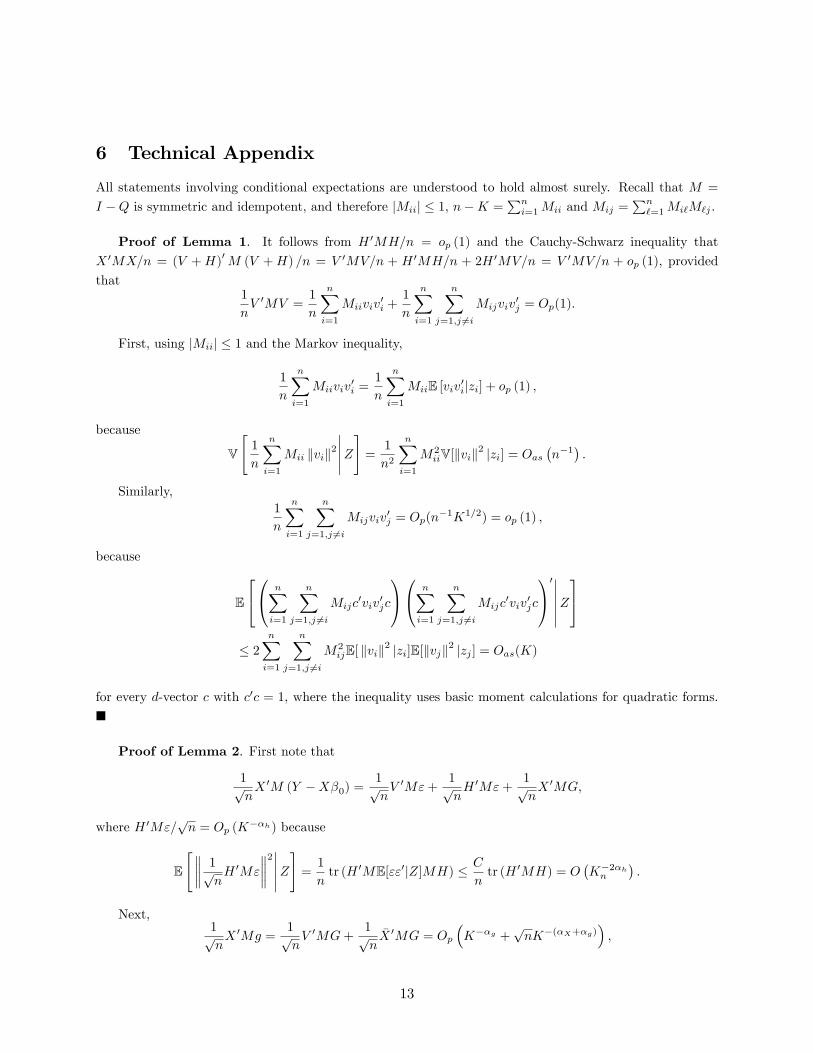
6 Technical Appendix

All statements involving conditional expectations are understood to hold almost surely. Recall that M =

I Q is symmetric and idempotent, and therefore jMiij 1, nK =Pn

i=1Mii and Mij =Pn

`=1Mi`M`j .

Proof of Lemma 1. It follows from H 0MH=n = op (1) and the Cauchy-Schwarz inequality that

X 0MX=n = (V +H)0M (V +H) =n = V 0MV=n + H 0MH=n + 2H 0MV=n = V 0MV=n + op (1), provided

that1

nV 0MV =

1

n

nXi=1

Miiviv0i +

1

n

nXi=1

nXj=1;j 6=i

Mijviv0j = Op(1).

First, using jMiij 1 and the Markov inequality,

1

n

nXi=1

Miiviv0i =

1

n

nXi=1

MiiE [viv0ijzi] + op (1) ,

because

V

"1

n

nXi=1

Mii kvik2Z#=1

n2

nXi=1

M2iiV[kvik

2 jzi] = Oasn1

.

Similarly,1

n

nXi=1

nXj=1;j 6=i

Mijviv0j = Op(n

1K1=2) = op (1) ,

because

E

240@ nXi=1

nXj=1;j 6=i

Mijc0viv

0jc

1A0@ nXi=1

nXj=1;j 6=i

Mijc0viv

0jc

1A0Z35

2nXi=1

nXj=1;j 6=i

M2ijE[ kvik

2 jzi]E[kvjk2 jzj ] = Oas(K)

for every d-vector c with c0c = 1, where the inequality uses basic moment calculations for quadratic forms.

Proof of Lemma 2. First note that

1pnX 0M (Y X0) =

1pnV 0M"+

1pnH 0M"+

1pnX 0MG,

where H 0M"=pn = Op (K

h) because

E

" 1pnH 0M"

2Z#=1

ntr (H 0ME[""0jZ]MH) C

ntr (H 0MH) = O

K2hn

.

Next,1pnX 0Mg =

1pnV 0MG+

1pnX 0MG = Op

Kg +

pnK(X+g)

,

13

because

E

" 1pnV 0MG

2Z#=1

nG0ME [V V 0jZ]MG C

nG0MG = Oas

K2g

,

and1pnH 0MG

pn

r1

nH 0MH

r1

nG0MG = Oas

pnK(X+g)

,

which completes the proof.

Lemma 4. Suppose E[ kVik4 jZi] < CV <1 and E"4i jZi

< C" <1 (a.s.). If 1Qii > FQ > 0 (a.s.)

and if min (n) > F > 0; then

1=2n

1pnV 0(I Q)"!d N (0; Id) .

Proof of Lemma 4. Use Lemma A2 in Chao, Swanson, Hausman, Newey, and Woutersen (2009).

Proof of Theorem 2. First, it follows from G0MG=n = op (1) and the Cauchy-Schwarz inequality that

1

n"0" =

1

n(Y X)0M(Y X)

=1

n(Y X G)0M(Y X G) + 1

nG0MG 2

n(Y X G)0MG

=1

n(Y X G)0M(Y X G) + op(1),

provided (Y X G)0M(Y X G)=n = Op (1). Next, note that Lemma 1 and = op(1) imply

( )0X 0MX( )=n = op (1), which together with the Cauchy-Schwarz inequality gives

1

n(Y X G)0M(Y X G)

=1

n"0M"+

1

n( )0X 0MX( ) 2

n(Y X( )G)0M( )

=1

n"0M"+ op(1) =

1

n~"0~"+ op(1).

Finally, consider the bilinear form

1

n~"0~" =

1

n"0M" =

1

n

nXi=1

Mii"2i +

1

n

nXi=1

nXj=1;j 6=i

"iMij"j .

First, using jMiij 1 and the fact that Sn = E [SnjZ] +Op(E [V [SnjZ]])1=2

,

1

n

nXi=1

Mii"2i =

1

n

nXi=1

MiiE"2i jzi

+ op (1) =

nKn

2 + op(1),

14

because

E

"V

"1

n

nXi=1

Mii"2i

Z##= E

"1

n2

nXi=1

M2iiV["2i jzi]

# 1

n2

nXi=1

EV["2i jzi]

CV

n= o (1) .

Second, using similar arguments,

1

n

nXi=1

nXj=1;j 6=i

Mij"i"j = Op

n1K1=2

= op (1) ,

because

E

2640@ 1n

nXi=1

nXj=1;j 6=i

Mij"i"j

1A2Z375 = 2

n2

nXi=1

nXj=1;j 6=i

M2ijE["2i jzi]E["2j jzj ]

2CVK

n2.

Therefore, because (nK)=(nK d)! 1,

2 =1

nK d "0" = 2 + op(1),

which completes the proof.

Proof of Theorem 3. Special case of Theorem 4.

Proof of Theorem 4. Available upon request.

15

References

Abadie, A., and G. W. Imbens (2006): Large Sample Properties of Matching Estimators for Average

Treatment E¤ects,Econometrica, 74(1), 235267.

Cattaneo, M. D., R. K. Crump, and M. Jansson (2010): Small Bandwidth Asymptotics for Density-

Weighted Average Derivatives,working paper.

Chao, J. C., N. R. Swanson, J. A. Hausman, W. K. Newey, and T. Woutersen (2009): Asymptotic

Distribution of JIVE in a Heteroskedastic IV Regression with Many Instruments,working paper.

Chen, X. (2007): Large Sample Sieve Estimation of Semi-Nonparametric Models,in Handbook of Econo-

metrics, Volume VI, ed. by J. Heckman, and E. Leamer, pp. 55505632. Elsevier Science B.V.

Donald, S. G., and W. K. Newey (1994): Series Estimation of Semilinear Models,Journal of Multi-

variate Analysis, 50(1), 3040.

Hansen, C., J. Hausman, and W. K. Newey (2008): Estimation with Many Instrumental Variables,

Journal of Business and Economic Statistics, 26(4), 398422.

Linton, O. (1995): Second Order Approximation in the Partialy Linear Regression Model,Econometrica,

63(5), 10791112.

Newey, W. K. (1997): Convergence Rates and Asymptotic Normality for Series Estimators,Journal of

Econometrics, 79, 147168.

Newey, W. K., and D. McFadden (1994): Large Sample Estimation and Hypothesis Testing, in

Handbook of Econometrics, Volume IV, ed. by R. F. Engle, and D. L. McFadden, pp. 21122245. Elsevier

Science B.V.

Robinson, P. M. (1988): Root-N-Consistent Semiparametric Regression,Econometrica, 56(4), 931954.

16

0.0

0.1

0.2

0.3

0.4

0.5

0.6

0.7

0.8

0.9

1.0

Mo

del

1

Kn

Empirical Coverage

0.95

VH

O1

VH

O2

VH

R1

VH

R2

VC

JN

1

VC

JN

2

0.0

0.1

0.2

0.3

0.4

0.5

0.6

0.7

0.8

0.9

1.0

Mo

del

2

Kn

Empirical Coverage

0.95

0.0

0.1

0.2

0.3

0.4

0.5

0.6

0.7

0.8

0.9

1.0

Mo

del

3

Kn

Empirical Coverage

0.95

0.0

0.1

0.2

0.3

0.4

0.5

0.6

0.7

0.8

0.9

1.0

Mo

del

4

Kn

Empirical Coverage

0.95

Figure1:EmpiricalCoverageRatesfor95%CondenceIntervals:n=500,S=3;000

17

matias d. cattaneo department of economics, …econ.msu.edu/seminars/docs/matias...

Documents