Team Cornell’s Skynet: Challenges and Achievements in Urban

Perception and Planning

Speaker:

Isaac MillerTeam Leaders:

Mark Campbell, Dan Huttenlocher

2 of 21

Team Cornell’s “Skynet”

• 2007 Chevrolet Tahoe: steering, throttle, brake, transmission actuated• Front sensing: 3 Ibeo LIDARs, 5 Delphi radars, 2 optical cameras• Back sensing: 1 SICK LIDAR, 3 Delphi radars, 1 optical camera

Delphi millimeter- wave radar

Ibeo LIDAR

Basler optical camera

Velodyne LIDAR

SICK LIDAR

3 of 21

Team Cornell’s “Skynet”

• Litton LN-200 tactical grade inertial measurement unit (IMU)• Stock GM ABS wheel encoders, 64 count / revolution• Septentrio PolaRx2e@ 3-antenna GPS / WAAS receiver• Trimble Ag252 high precision (HP) differential corrections receiver

Septentrio PolaRx2e@

Trimble Ag252

GM ABS wheel

encoder

Litton LN- 200 IMU

4 of 21

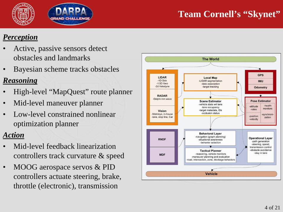
Team Cornell’s “Skynet”

Perception• Active, passive sensors detect

obstacles and landmarks• Bayesian scheme tracks obstaclesReasoning• High-level “MapQuest” route planner• Mid-level maneuver planner• Low-level constrained nonlinear

optimization plannerAction• Mid-level feedback linearization

controllers track curvature & speed• MOOG aerospace servos & PID

controllers actuate steering, brake, throttle (electronic), transmission

5 of 21

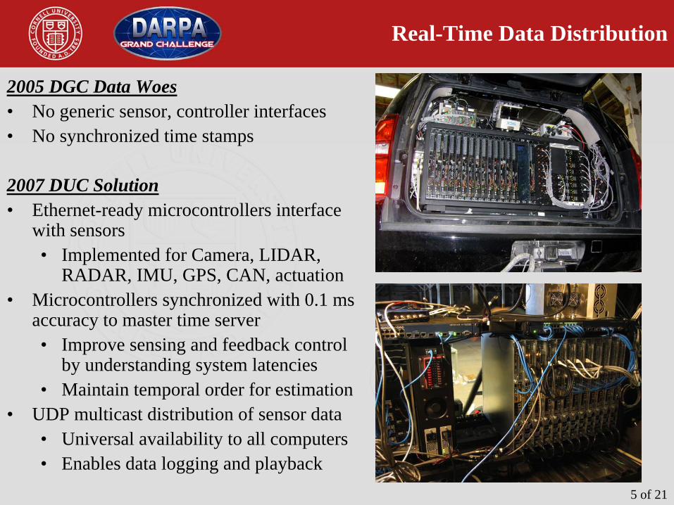
Real-Time Data Distribution

2005 DGC Data Woes• No generic sensor, controller interfaces• No synchronized time stamps

2007 DUC Solution• Ethernet-ready microcontrollers interface

with sensors• Implemented for Camera, LIDAR,

RADAR, IMU, GPS, CAN, actuation• Microcontrollers synchronized with 0.1 ms

accuracy to master time server• Improve sensing and feedback control

by understanding system latencies• Maintain temporal order for estimation

• UDP multicast distribution of sensor data• Universal availability to all computers• Enables data logging and playback

6 of 21

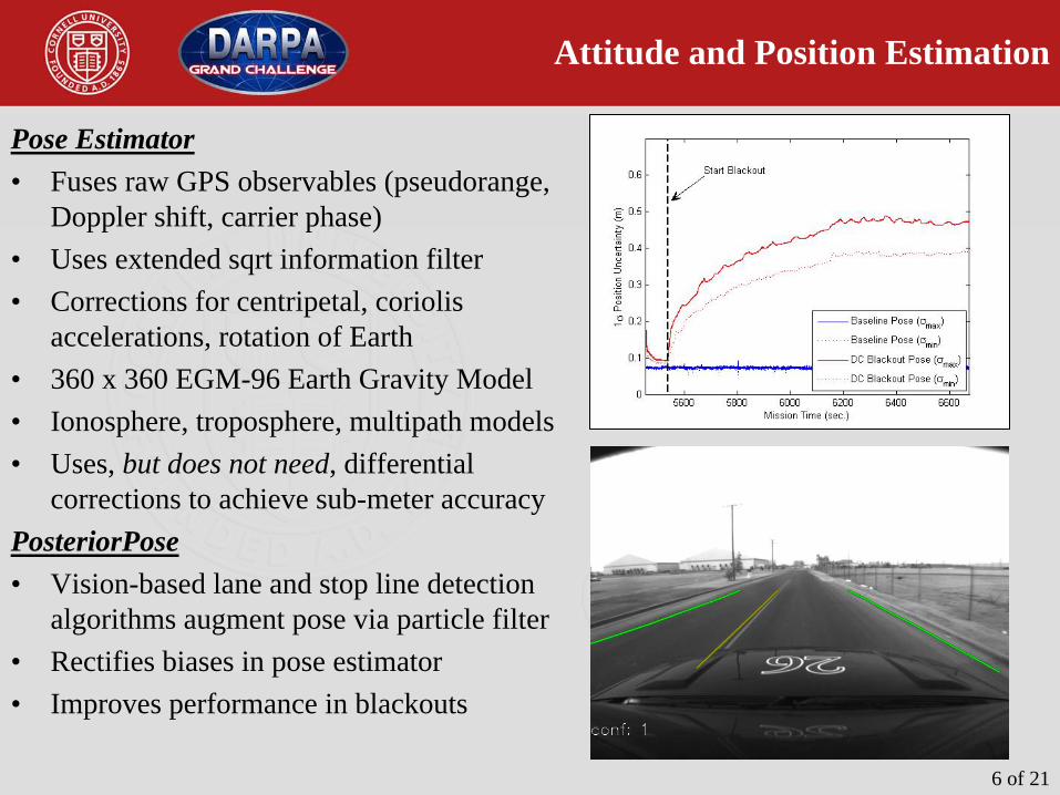
Attitude and Position Estimation

Pose Estimator• Fuses raw GPS observables (pseudorange,

Doppler shift, carrier phase)• Uses extended sqrt information filter• Corrections for centripetal, coriolis

accelerations, rotation of Earth• 360 x 360 EGM-96 Earth Gravity Model• Ionosphere, troposphere, multipath models• Uses, but does not need, differential

corrections to achieve sub-meter accuracyPosteriorPose• Vision-based lane and stop line detection

algorithms augment pose via particle filter• Rectifies biases in pose estimator• Improves performance in blackouts

7 of 21

Obstacle Detection and Tracking

Algorithm Overview1. Segmenting sensor data2. Determining number of obstacles /

assigning measurements3. Tracking obstacles4. Determining tracked object metadata 5. Maintaining stable track IDs

• Key design choice: obstacles not assumed to have structured motion

• Key design choice: interface between obstacle tracker / planner based on assigned obstacle identification tag

8 of 21

Obstacle Detection and Tracking

Segmenting Sensor Data• Multiple sensors (laser, radar, camera)

fused at object tracking level• Delphi radar tracks used “as is”• MobilEye camera tracks used “as is”• LIDAR detections segmented

• Grid-based ground model constructed from low-pass filtered LIDAR, similar to DGC ’05

• Ground model Skynet-centric• Subtract “obvious” static

environment using ground model• Remainder of points may still be

cars, must be considered further

Gray Unclassified

9 of 21

Obstacle Detection and Tracking

Clustering LIDAR Data• LIDAR obstacle points clustered into

objects via Euclidean distance• 1m spacing rule defines cluster bounds• Multi-threshold, single frame

clustering removes unstable clusters• Occlusion contours determined via

range reasoning• Stable measurements extracted

• Occlusion contour bearings• Range to closest point

• Key point: segmentation is brittle, so only extract measurements from distinct, stable objects

Gray Unclassified

Ego-vehicle

Stable clusters Unstable clustersGround hits

3 Ibeos, 12 colored laser beams

10 of 21

Obstacle Detection and Tracking

Determining the Number of Obstacles• Factorize over assignments N and

obstacle states O:

• Data assignment solved by particle filter

• Tracking solved by hybrid sigma point filters run for each obstacle in each particle

• Each particle is a complete hypothesis of the world – 4 for DUC

• Number of obstacles is determined automatically in the filter

• Inexpensive: particles are only used for measurement assignment

( ) ( ) ( )ZNOpZNpZONp ,, ⋅=( )ZNp

( )ZNOp ,

Tracked objects

Untracked obstacle points

11 of 21

Obstacle Detection and Tracking

Tracking Obstacles• Obstacle points stored in obstacle-centric frame, with floating origin• Obstacle state: 2d rigid body transform + ground speed, heading• EKF prediction integrates rigid body transform over time, sigma point update

compares predicted and measured points to update transform & velocity• Cluster points replaced after each update• Fixed measurement location (back axle or center of mass) not required

Tracked objects

12 of 21

Obstacle Detection and Tracking

Tracked Object Metadata• Raw tracking data too low-level• Planner needs behavior-level metadata

• HMM used to tell if car-like and whether stopped/disabled

• Monte Carlo sampling used for obstacle lane occupancy probabilities• Tracker predicts when obstacles

should be visible and when not• Occlusion reasoning persists

tracked obstacles when not visible• Obstacles only deleted when there’s

evidence they don’t existOccluded, stopped

Visible, stopped

Visible, moving

Ego-vehicle

13 of 21

Obstacle Detection and Tracking

Maintaining Track Identification• Track IDs generated from obstacles via global maximum likelihood matching to

previous frame given all measurements Z

• Stable cluster measurements used to match existing tracks with new obstacles• Dynamic programming solves correspondences efficiently• Persistent track IDs allow frame-to-frame reasoning in planner

( ) ( ) ( )( )ZkOkOpkO ii

=+=+ 1maxarg1

Tracked obstacles

Untracked points

Ego vehicle

14 of 21

Obstacle Detection and Tracking

15 of 21

Intelligent Planning

• Decision making and execution• Behavioral (macro planning): route planning, replanning• Tactical (local planning): changing lanes, passing, intersections, merging• Operational (plan execution): path generation

• Robust against unforeseen, complex scenarios

16 of 21

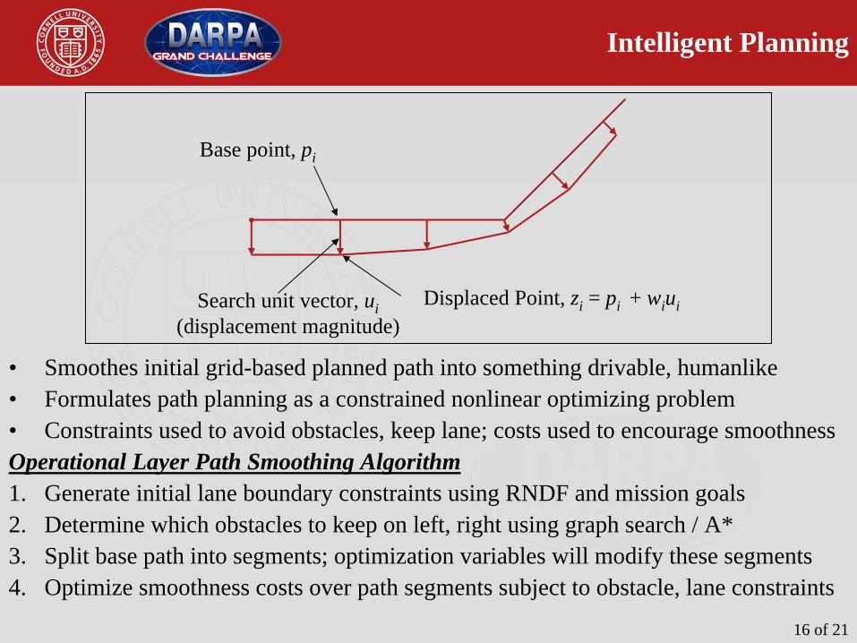
Intelligent Planning

• Smoothes initial grid-based planned path into something drivable, humanlike• Formulates path planning as a constrained nonlinear optimizing problem• Constraints used to avoid obstacles, keep lane; costs used to encourage smoothnessOperational Layer Path Smoothing Algorithm1. Generate initial lane boundary constraints using RNDF and mission goals2. Determine which obstacles to keep on left, right using graph search / A*3. Split base path into segments; optimization variables will modify these segments4. Optimize smoothness costs over path segments subject to obstacle, lane constraints

Base point, pi

Search unit vector, ui(displacement magnitude)

Displaced Point, zi = pi + wi ui

17 of 21

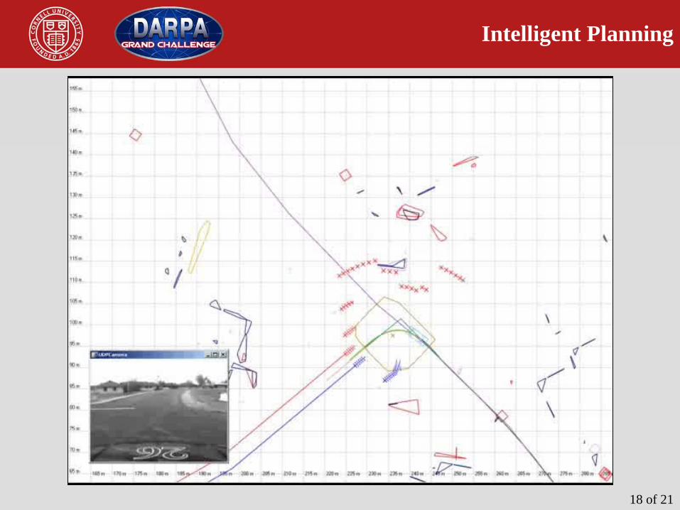
Intelligent Planning

RNDF

Laneboundaries

Convex hulls of obstacles

Ego- vehicle

Plannerconstraints

Constraints around parked car

18 of 21

Intelligent Planning

19 of 21

Overall DUC Statistics

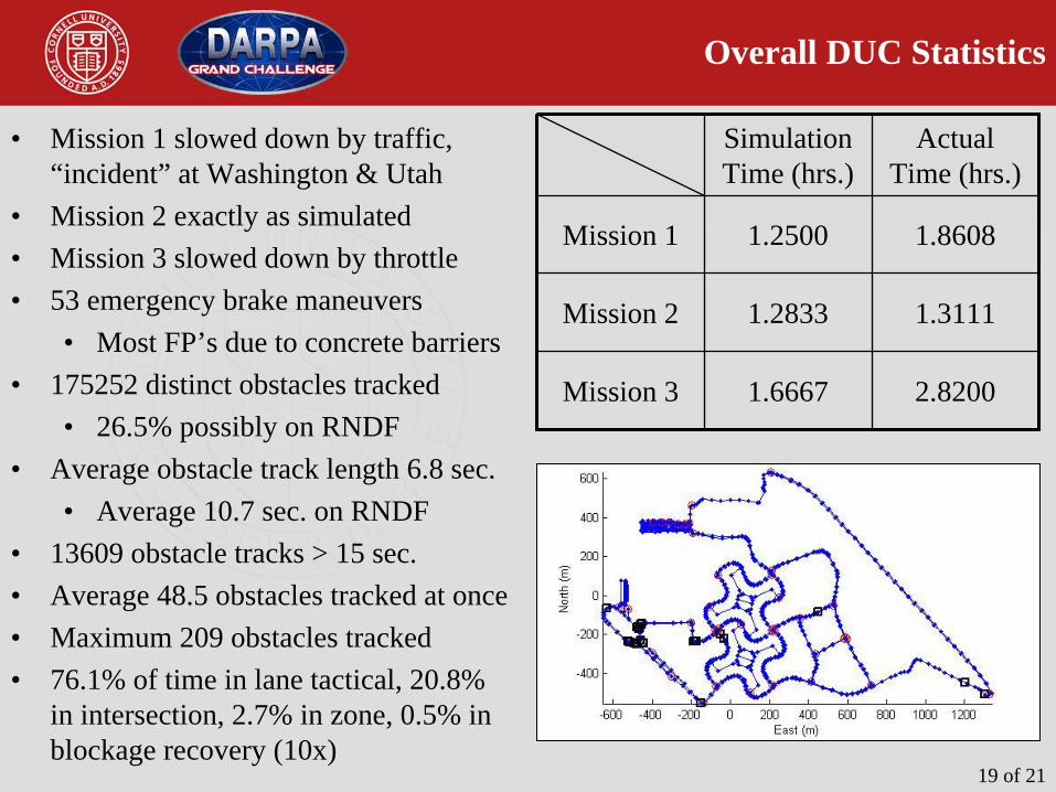
• Mission 1 slowed down by traffic, “incident” at Washington & Utah

• Mission 2 exactly as simulated• Mission 3 slowed down by throttle• 53 emergency brake maneuvers

• Most FP’s due to concrete barriers• 175252 distinct obstacles tracked

• 26.5% possibly on RNDF• Average obstacle track length 6.8 sec.

• Average 10.7 sec. on RNDF• 13609 obstacle tracks > 15 sec.• Average 48.5 obstacles tracked at once• Maximum 209 obstacles tracked• 76.1% of time in lane tactical, 20.8%

in intersection, 2.7% in zone, 0.5% in blockage recovery (10x)

Simulation Time (hrs.)

Actual Time (hrs.)

Mission 1 1.2500 1.8608

Mission 2 1.2833 1.3111

Mission 3 1.6667 2.8200

20 of 21

Even When Everything Goes Right…

21 of 21

Lessons Learned

• Synchronization and accurate time stamps permit stable tracking• Accurate, continuous pose estimator foundation of successful driving• Fusion of multiple data sources, including vision, important for

vehicle localization• Sensor segmentation algorithms are brittle at best

• Model the ground to remove ground hits for better clustering• Stable clusters not enough, need stable measurements

• Evidence from raw sensors cleans up tracking mistakes• Stable track metadata critical for high level reasoning• Constrained optimization mature enough for real-world path planning• Deterministic high-level reasoning is delicate for urban driving• Many single points of failure inevitable; must understand the risks