tdem surveying

TIME-DOMAIN ELECTROMAGNETIC

SURVEYING(TDEM)

Summary

Suska Ulin Agusta

Trainee Geophysicist

[email protected]

Khumsup Pty Ltd

2012

04/11/2023Suska Ulin Agusta | Khumsup Pty Ltd 2

OUTLINE Introduction The Phenomenon Measurement Mathematics Data Quality Good Field Data Acquisition

Practices Data Processing Data Interpretation Applicability Airborne TDEM Borehole TDEM References


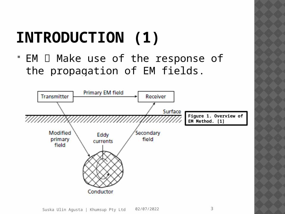
INTRODUCTION (1) EM Make use of the response of the

propagation of EM fields.

Figure 1. Overview of EM Method. [1]


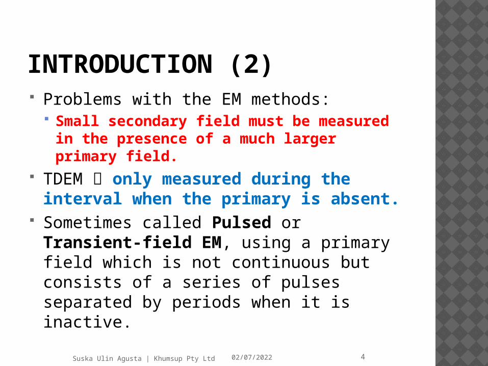
INTRODUCTION (2) Problems with the EM methods:

Small secondary field must be measured in the presence of a much larger primary field.

TDEM only measured during the interval when the primary is absent.

Sometimes called Pulsed or Transient-field EM, using a primary field which is not continuous but consists of a series of pulses separated by periods when it is inactive.


Applications of Time-Domain Electromagnetic (TDEM) Techniques Determining electrical conductivity

of soils at depth 30 feet – 3000 feet Mapping soils and changes in soil

types in that depth of range Mapping sand and gravel aquifers Mapping clayey layers restricting

ground-water flow Mapping conductive leachate in

groundwater Mapping salt water intrusion Determining the depth of the

bedrock

INTRODUCTION (3)


Ampere’s law with Maxwell’s correction states that magnetic field can be generated in two ways: by electrical current by changing electric fields

The correction shows that not only a changing

magnetic field induces an electric field,

but also a changing electric field induces a magnetic field.

THE PHENOMENON (1)

Figure 2. Electromagnetic Induction caused by electrical current (taken from http://www.google.co.id/imghp?hl=id&tab=wi)


All moving charged particles produce magnetic fields.

Magnetic field lines form in concentric circles around a cylindrical current-carrying conductor, such as a length of wire. The direction of such a magnetic field can be determined by using the "right hand grip rule" (see figure at right).

THE PHENOMENON (2)

Figure 3. Right hand grip rule. taken from http://www.google.co.id/imghp?hl=id&tab=wi

http://en.wikipedia.org/wiki/Concentric

http://en.wikipedia.org/wiki/Cylinder_(geometry)

http://en.wikipedia.org/wiki/Right_hand_grip_rule


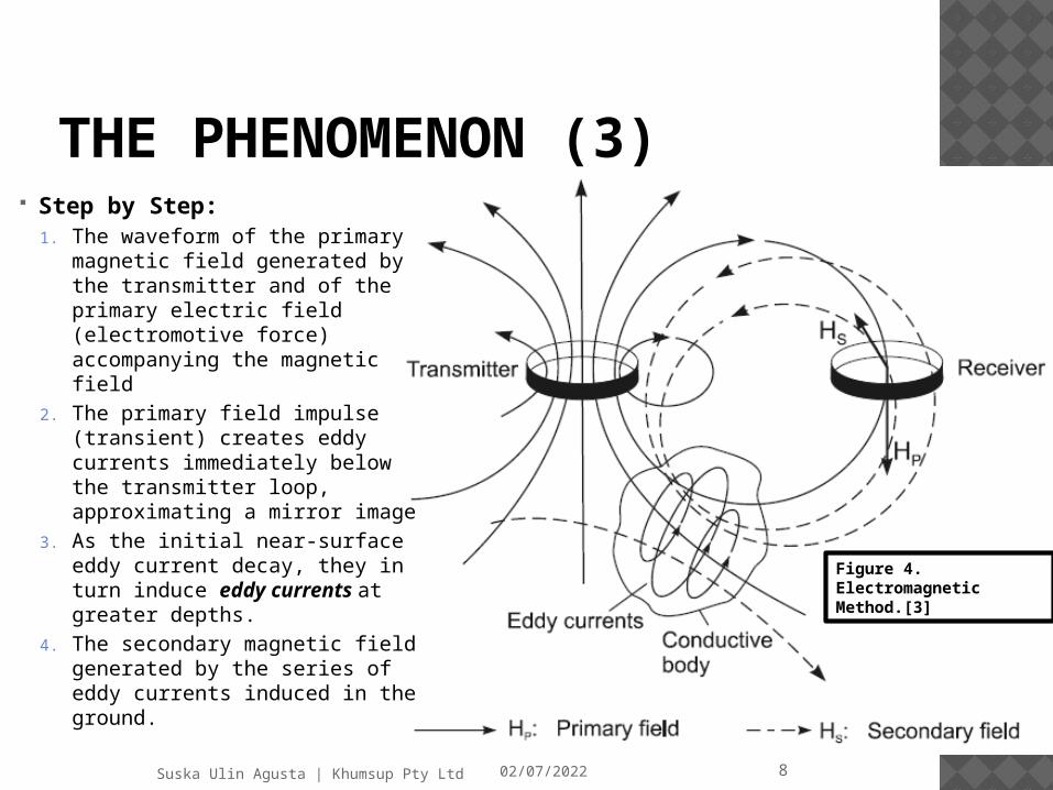
Figure 4. Electromagnetic Method.[3]

THE PHENOMENON (3) Step by Step:

1. The waveform of the primary magnetic field generated by the transmitter and of the primary electric field (electromotive force) accompanying the magnetic field

2. The primary field impulse (transient) creates eddy currents immediately below the transmitter loop, approximating a mirror image

3. As the initial near-surface eddy current decay, they in turn induce eddy currents at greater depths.

4. The secondary magnetic field generated by the series of eddy currents induced in the ground.


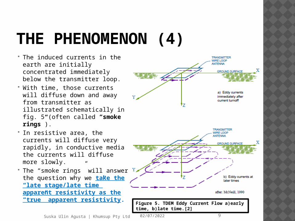
THE PHENOMENON (4) The induced currents in the earth

are initially concentrated immediately below the transmitter loop.

With time, those currents will diffuse down and away from transmitter as illustrated schematically in fig. 5 (often called “smoke rings”).

In resistive area, the currents will diffuse very rapidly, in conductive media the currents will diffuse more slowly.

The “smoke rings” will answer the question why we take the “late stage/late time” apparent resistivity as the “true” apparent resistivity. Figure 5. TDEM Eddy Current Flow a)early time,

b)late time.[2]


Main Equipments TEM Transmitter

Specifications include: current waveform, base frequency (Hz), turn-off time (μs), transmitter loop (in single turn loop & 8-turn loop), output voltage (V), power supply (V, rechargeable/not), battery life, weight, and dimensions.

TEM Receiver + Antenna

Specifications include: rate of decay induced magnetic field (nV/m2), EM sensor, channels, time gates, dynamic range (bits), base frequency (Hz), integration time (s), display (dot graphic LCD), memory, synchronization, power supply, weight, dimensions.

Loop of Wires Rx Coil Generator/power supply (if needed)

MEASUREMENT (1)


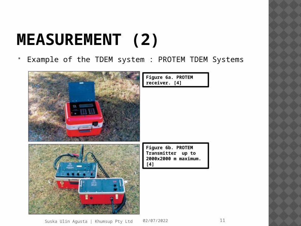
MEASUREMENT (2) Example of the TDEM system : PROTEM TDEM Systems

Figure 6a. PROTEM receiver. [4]

Figure 6b. PROTEM Transmitter up to 2000x2000 m maximum.[4]


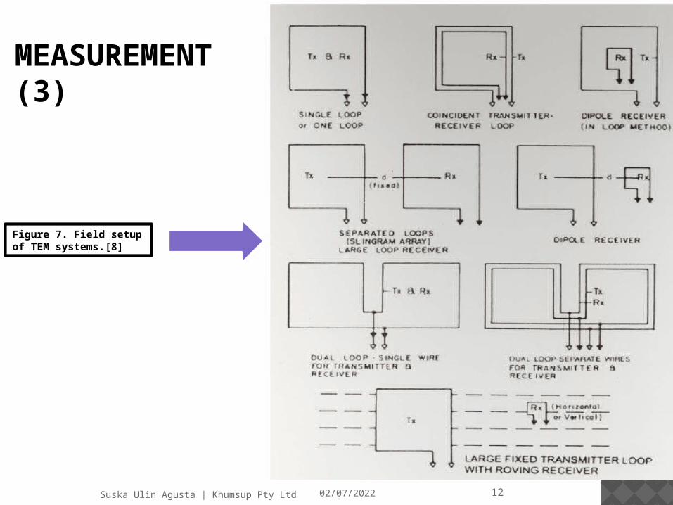
MEASUREMENT (3)

Figure 7. Field setup of TEM systems.[8]


MEASUREMENT (4) Figure 5 shows a typical for a “central loop”

TDEM sounding.

Figure 8. TDEM field configuration2].


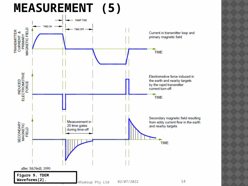
MEASUREMENT (5)

Figure 9. TDEM Waveforms[2].


After each measurement, the sign changes in the primary magnetic field are applied for suppression of:1. The coherent noise signals from power lines, if

the repetition frequency is chosen as a sub harmonics of the power line frequency

2. Offsets of the instrumental amplifiers

This measuring technique is referred to as synchronous detection

MEASUREMENT (6)


The datasets are recorded in decay time windows often called gates (dB/dt) the time derivative of the magnetic flux passing the coil).

The gates arranged with a logarithmically increasing width to improve the signal/noise (S/N) ratio especially at late times.

S/N ratio compares the level of a desired signal to the level of background noise.

This is called “Log-Gating” and 8-10 gates per decade in decay time are commonly used.

MEASUREMENT (7)

Figure 10. The quantification of a decaying TDEM response by measurement of its amplitude in a number of channels (1-6) at increasing times (t1-6) after primary field cut-off. The amplitudes of the response in the different channels are recorded along a profile.[1]


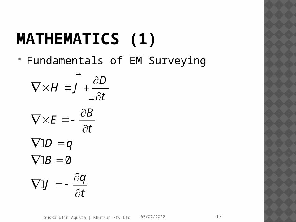
Fundamentals of EM Surveying

MATHEMATICS (1)

0

DH J

t

BE

tD q

B

qJ

t


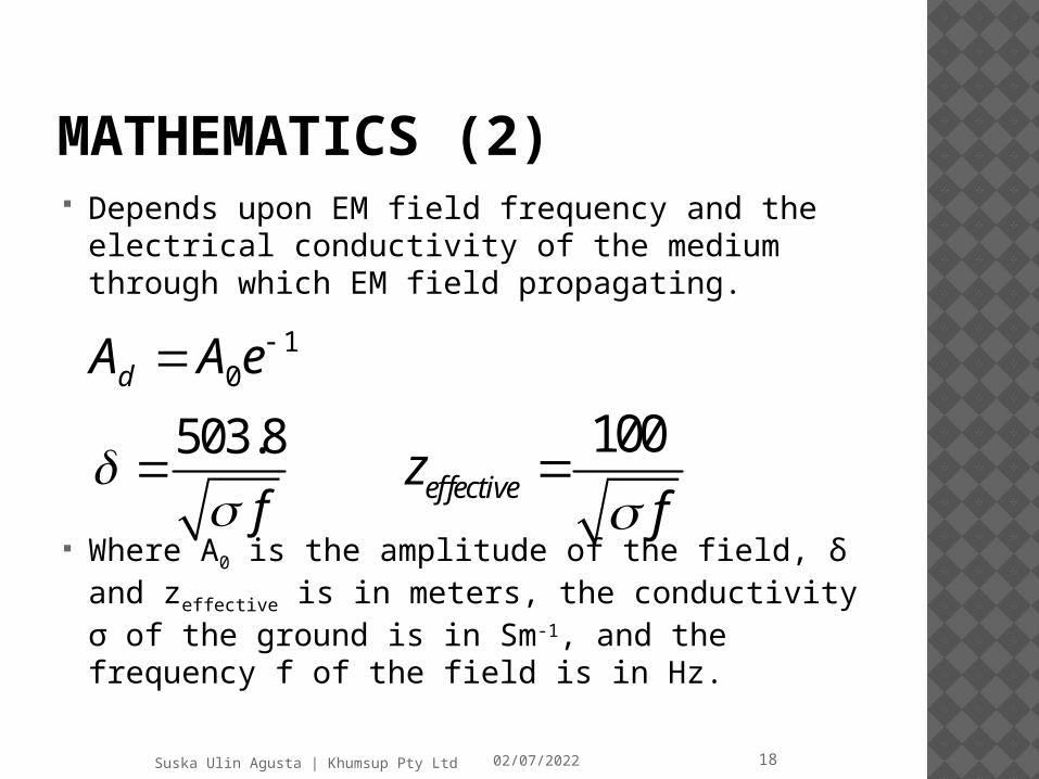
Depends upon EM field frequency and the electrical conductivity of the medium through which EM field propagating.

Where A0 is the amplitude of the field, δ and zeffective is in meters, the conductivity σ of the ground is in Sm-1, and the frequency f of the field is in Hz.

10dA A e

503.8

f

100effectivez

f

MATHEMATICS (2)


The decaying secondary magnetic field is referred to b or the step response.

The actual measurement is that of db/dt. Is called the impulse response.

At late-times, the impulse response can be written as:

As seen db/dt has a decay development proportional to t-5/2.

MATHEMATICS (3)

3/2 5/2 25/20

1/220z I ab

tt

Figure 11. In the impulse responses (db/dt) for a homogeneous halfspace with varying resistivities are presented.[5]


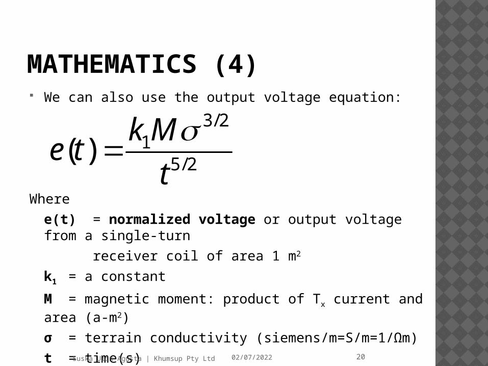
We can also use the output voltage equation:

Where

e(t) = normalized voltage or output voltage from a single-turn

receiver coil of area 1 m2

k1 = a constant

M = magnetic moment: product of Tx current and area (a-m2)

σ = terrain conductivity (siemens/m=S/m=1/Ωm)

t = time(s)

MATHEMATICS (4)

3/21

5/2( )

k Me t

t


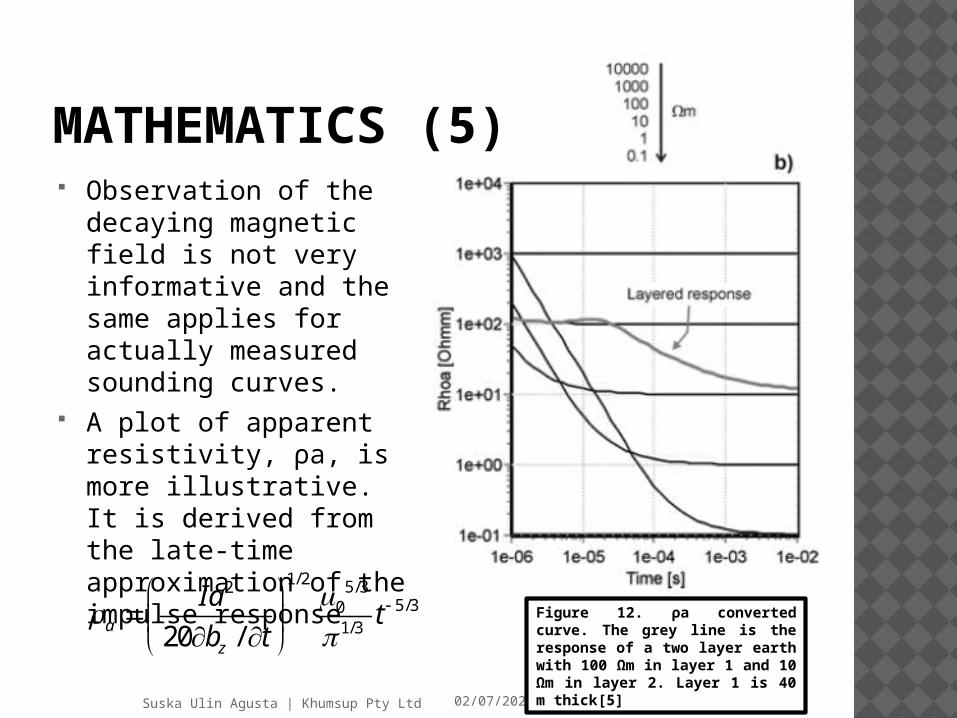
Observation of the decaying magnetic field is not very informative and the same applies for actually measured sounding curves.

A plot of apparent resistivity, ρa, is more illustrative. It is derived from the late-time approximation of the impulse response

MATHEMATICS (5)

1/2 5/325/30

1/320 /az

Iat

b t

Figure 12. ρa converted curve. The grey line is the response of a two layer earth with 100 Ωm in layer 1 and 10 Ωm in layer 2. Layer 1 is 40 m thick[5]


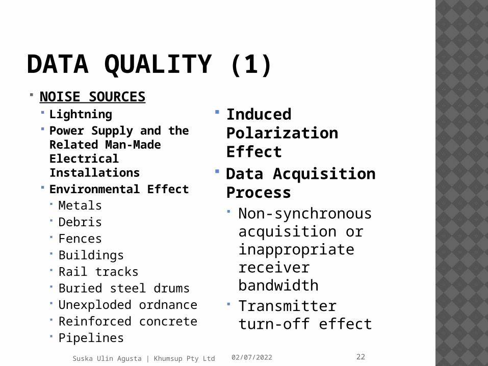
DATA QUALITY (1) NOISE SOURCES

Lightning Power Supply and the

Related Man-Made Electrical Installations

Environmental Effect Metals Debris Fences Buildings Rail tracks Buried steel drums Unexploded ordnance Reinforced concrete Pipelines

Induced Polarization Effect

Data Acquisition Process Non-synchronous

acquisition or inappropriate receiver bandwidth

Transmitter turn-off effect


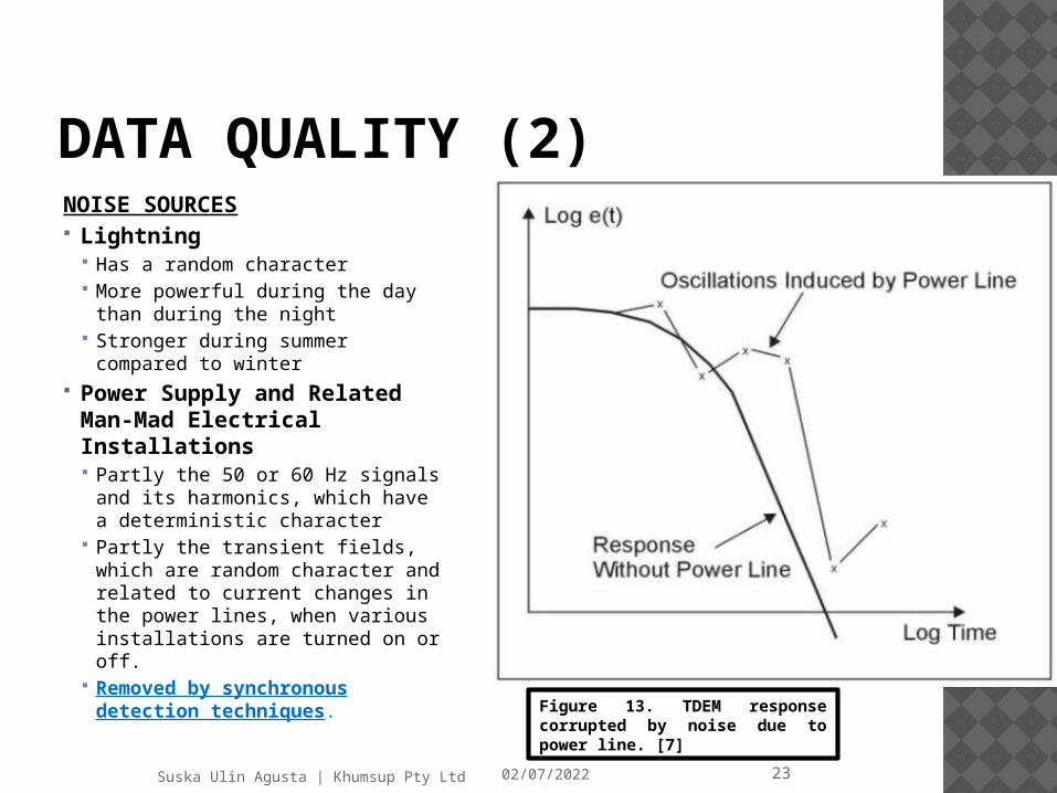
DATA QUALITY (2)NOISE SOURCES Lightning

Has a random character More powerful during the day than

during the night Stronger during summer compared

to winter Power Supply and Related

Man-Mad Electrical Installations Partly the 50 or 60 Hz signals and

its harmonics, which have a deterministic character

Partly the transient fields, which are random character and related to current changes in the power lines, when various installations are turned on or off.

Removed by synchronous detection techniques.

Figure 13. TDEM response corrupted by noise due to power line. [7]


NOISE SOURCES Environmental Effect

Example: Presence of small metal objects, or “clutter”.

We can see that the very-late time TDEM Signals are virtually free of geologic and clutter-generated noise.

DATA QUALITY (3)

Figure 14. The TDEM response of a vertical buried plate target with clutter. Solid dots indicate response without clutter. Solid lines indicate responses with 5 different realizations of clutter. Each plot shows the spatial response at a single time gate.[6]


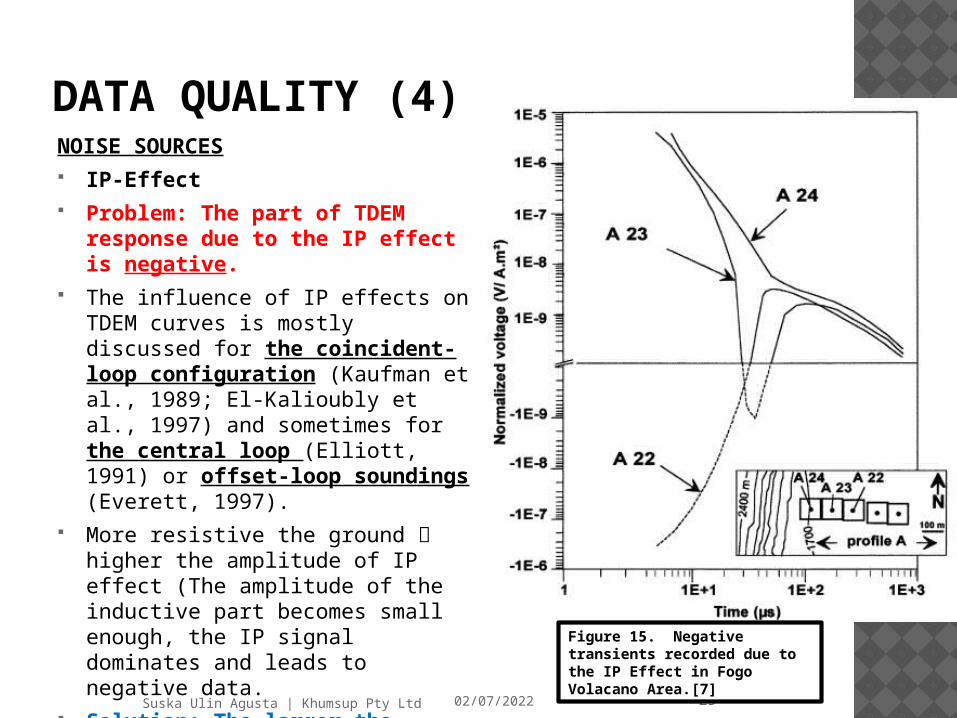
NOISE SOURCES IP-Effect Problem: The part of TDEM response

due to the IP effect is negative. The influence of IP effects on TDEM

curves is mostly discussed for the coincident-loop configuration (Kaufman et al., 1989; El-Kalioubly et al., 1997) and sometimes for the central loop (Elliott, 1991) or offset-loop soundings (Everett, 1997).

More resistive the ground higher the amplitude of IP effect (The amplitude of the inductive part becomes small enough, the IP signal dominates and leads to negative data.

Solution: The larger the transmitter loop, the less predominant the IP Effect should be.

DATA QUALITY (4)

Figure 15. Negative transients recorded due to the IP Effect in Fogo Volacano Area.[7]


NOISE SOURCES Data Acquisition Process

Non-synchronous acquisition or inappropriate receiver bandwidth

1. Could lead to the fact that the first windows of the transient should have been registered during the turn-off of the primary signal.

2. A limited receiver bandwidth could integrate the receiver response to the primary field so it extends into the time window of early measurements.

EFFECT: An increasing amplitude of early time positive measurements, but never in reversing their polarity delayed response.

DATA QUALITY (5)


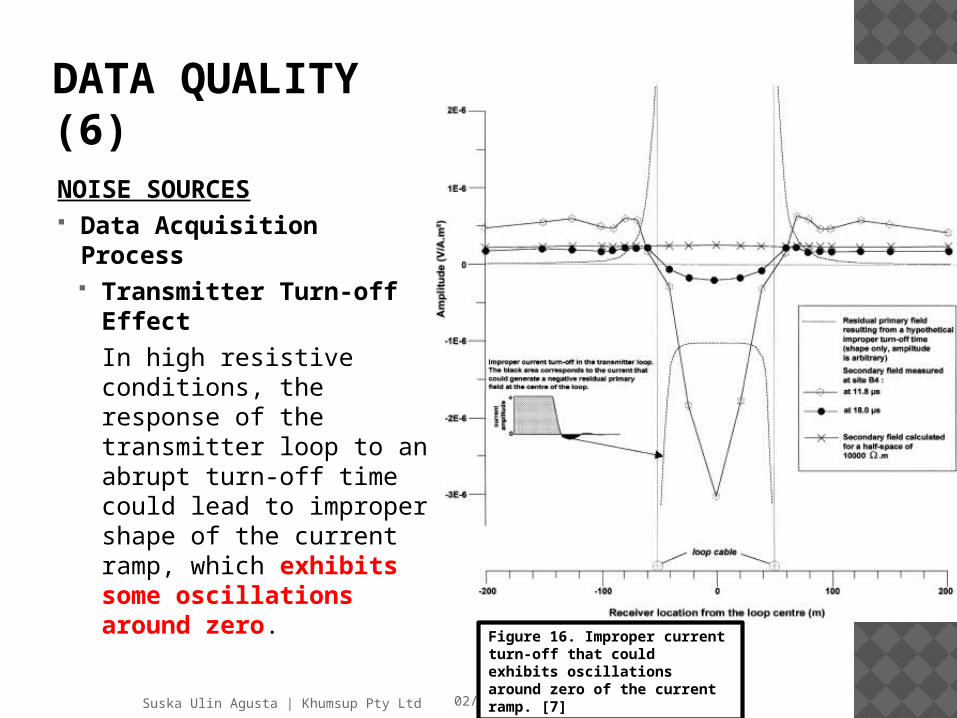
NOISE SOURCES Data Acquisition

Process Transmitter Turn-off

Effect

In high resistive conditions, the response of the transmitter loop to an abrupt turn-off time could lead to improper shape of the current ramp, which exhibits some oscillations around zero.

DATA QUALITY (6)

Figure 16. Improper current turn-off that could exhibits oscillations around zero of the current ramp. [7]


GOOD FIELD DATA ACQUISITION PRACTICES (1) Important element of the data quality precise

knowledge of the parameters of the applied instrument. Timing parameters must be known accurately

because of their severe impact on “early-time” data.

The geometry of the transmitter-receiver configuration must be accurate, especially for the offset-loop configuration.

Beware of the metal objects, buildings, fences, etc near the observation area.

High resistive area is not going to give a good recorded data.


A small transmitter coil with a high current is very field efficient, but 3 issues must be tackled in the configuration design: Saturated amplifiers will produce distorted signals for several

milliseconds.

Solution: Also use a large transmitter loop or a large offset between the transmitter and the receiver coils as a comparison.

The IP-effect.

Solution: Use offset configuration and moves to later decay-times as the offset between the transmitter and the receiver coil is increased.

At early times, measurements using the offset configuration are extremely sensitive to small variations in the resistivity in the near surface.

Solution: use central loop configuration that produces datasets which are less-affected by near-surface resistivity variations.

GOOD FIELD DATA ACQUISITION PRACTICES (2)


Borehole TDEM – Processing Short Manual

DATA PROCESSING (1)


What do the numbers that we work with mean? dB/dt or Impulse Response

The time derivative of the magnetic flux passing the coil is usually called “Normalized Voltage”. Output voltage which is normalized to a receiver coil

moment of 1-turn m2 (single turn with a coil area of square meter) and a transmitter current of 1 Ampere (A). Unit : μV/A, nV/m2, nV/Am2, V/A.

Apparent resistivity

A volume average of heterogeneous half-space.

Unit: Ω-m

DATA INTERPRETATION (1)


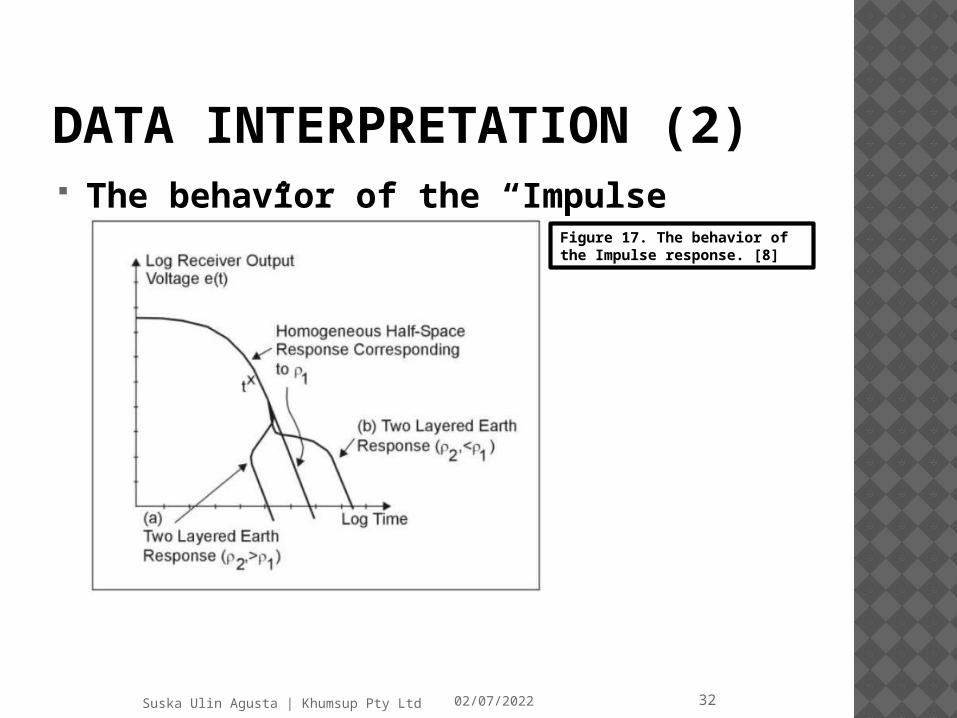
The behavior of the “Impulse Response”


Figure 17. The behavior of the Impulse response. [8]


The behavior of the “Apparent Resistivity” curves.


Figure 18. The behavior of the Apparent Resistivity. [8]


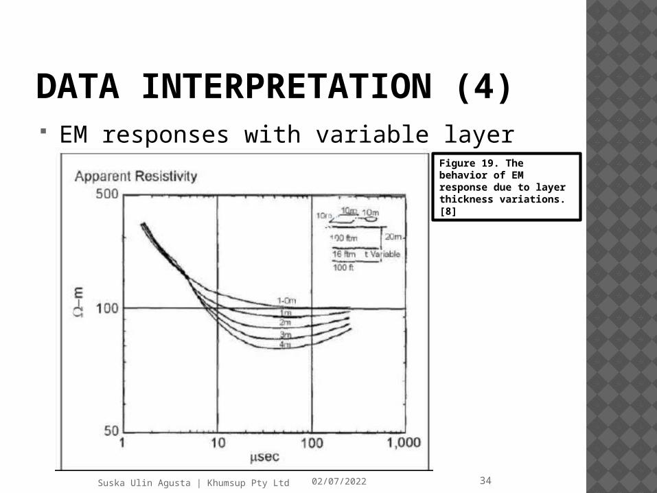
EM responses with variable layer thickness


Figure 19. The behavior of EM response due to layer thickness variations. [8]


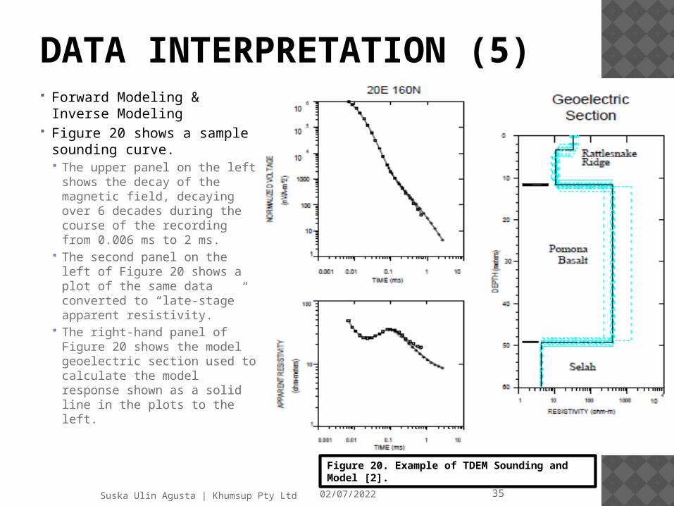
Forward Modeling & Inverse Modeling

Figure 20 shows a sample sounding curve. The upper panel on the left

shows the decay of the magnetic field, decaying over 6 decades during the course of the recording from 0.006 ms to 2 ms.

The second panel on the left of Figure 20 shows a plot of the same data converted to “late-stage” apparent resistivity.

The right-hand panel of Figure 20 shows the model geoelectric section used to calculate the model response shown as a solid line in the plots to the left.


Figure 20. Example of TDEM Sounding and Model [2].


1. Mineral Exploration – metallic elements are found in highly conductive massive sulfide ore bodies.

2. Groundwater Investigations – groundwater contaminants such as salts and acids significantly increase the groundwater conductivity.

3. Stratigraphy Mapping – rock types may have different conductivities.

4. Geothermal Energy – geothermal alteration due to hot water increases the conductivity of the host rock.

5. Permafrost Mapping – there is a significant conductivity contrast at the interface between frozen and unfrozen ground.

6. Environmental - locate hazards such as drums and tanks, contaminant plumes, etc.

APPLICABILITY (1)


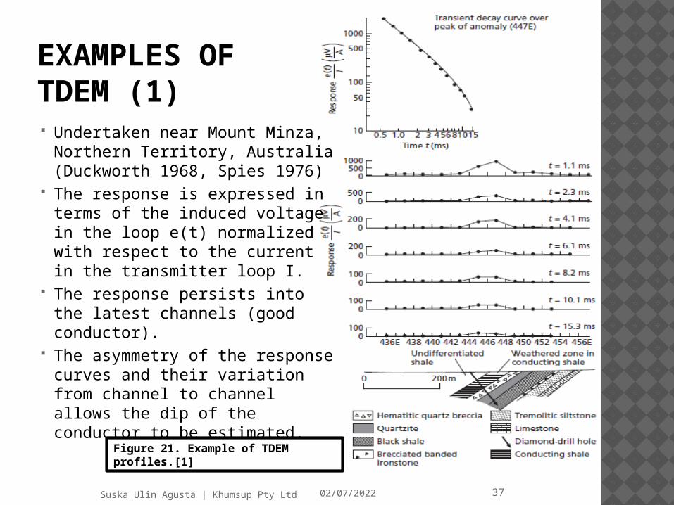
EXAMPLES OF TDEM (1) Undertaken near Mount Minza,

Northern Territory, Australia (Duckworth 1968, Spies 1976)

The response is expressed in terms of the induced voltage in the loop e(t) normalized with respect to the current in the transmitter loop I.

The response persists into the latest channels (good conductor).

The asymmetry of the response curves and their variation from channel to channel allows the dip of the conductor to be estimated.

Figure 21. Example of TDEM profiles.[1]


EXAMPLES OF TDEM (2) Borehole TDEM from the

Single Tree Hill area, NSW, Australia (Boyd & Wiles 1984)

In hole PDS1, the response at early times indicates the presence of a conductor at a depth of 145 m (negative response at later times diffusion of the eddy currents).

In hole DS1 and DS2, negative response respectively, indicate that the receiver passed outside, but near the edges of, the conductor at these depths.

A model consisting of a rectangular current-carrying loop. Figure 22. Borehole TDEM .[1]


Passive systems only the receiver is airborne. Include airborne versions of the VLF and AFMAG methods.

Active systems both transmitter and receiver are mobile. More commonly used Ground mobile transmitter-receiver systems lifted into the air

and interfaced with a continuous recording device. Comprise 2 main types: fixed separation & quadrature.

AIRBORNE TDEM (1)

Figure 23. Airborne EM Field Operation. [8]


Airborne TDEM Methods The discontinuous primary field is

generated by passing pulses of current through a transmitter coil strung about an aircraft.

The transient primary field induces currents persist during the period when the primary field is shut off and the receiver becomes active.

The exponential decay curve is sampled at several points and the signals displayed on a strip chart.

The signal amplitude in successive sampling channels is, to a certain extent, diagnostic of the type of conductor present.

Poor conductors produce a rapidly decaying voltage and only register on those channels sampling the voltage shortly after primary cut-off.

AIRBORNE TDEM (2)

Figure 24. Airborne EM schematic diagram.[8]


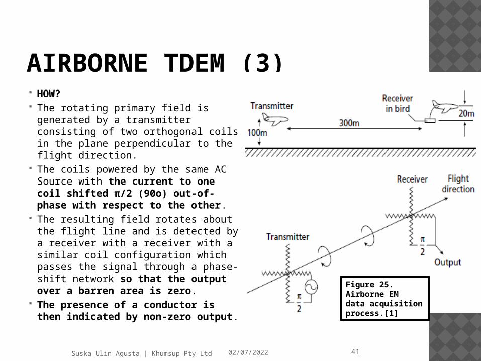
AIRBORNE TDEM (3) HOW? The rotating primary field is generated

by a transmitter consisting of two orthogonal coils in the plane perpendicular to the flight direction.

The coils powered by the same AC Source with the current to one coil shifted π/2 (90o) out-of-phase with respect to the other.

The resulting field rotates about the flight line and is detected by a receiver with a receiver with a similar coil configuration which passes the signal through a phase-shift network so that the output over a barren area is zero.

The presence of a conductor is then indicated by non-zero output.

Figure 25. Airborne EM data acquisition process.[1]


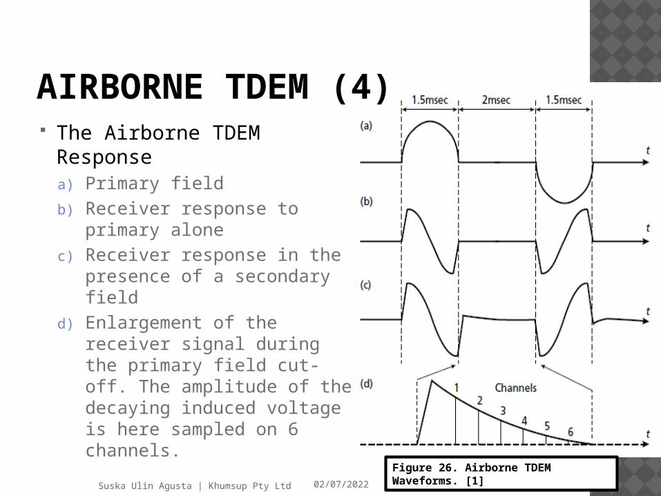
The Airborne TDEM Responsea) Primary field

b) Receiver response to primary alone

c) Receiver response in the presence of a secondary field

d) Enlargement of the receiver signal during the primary field cut-off. The amplitude of the decaying induced voltage is here sampled on 6 channels.

AIRBORNE TDEM (4)

Figure 26. Airborne TDEM Waveforms. [1]


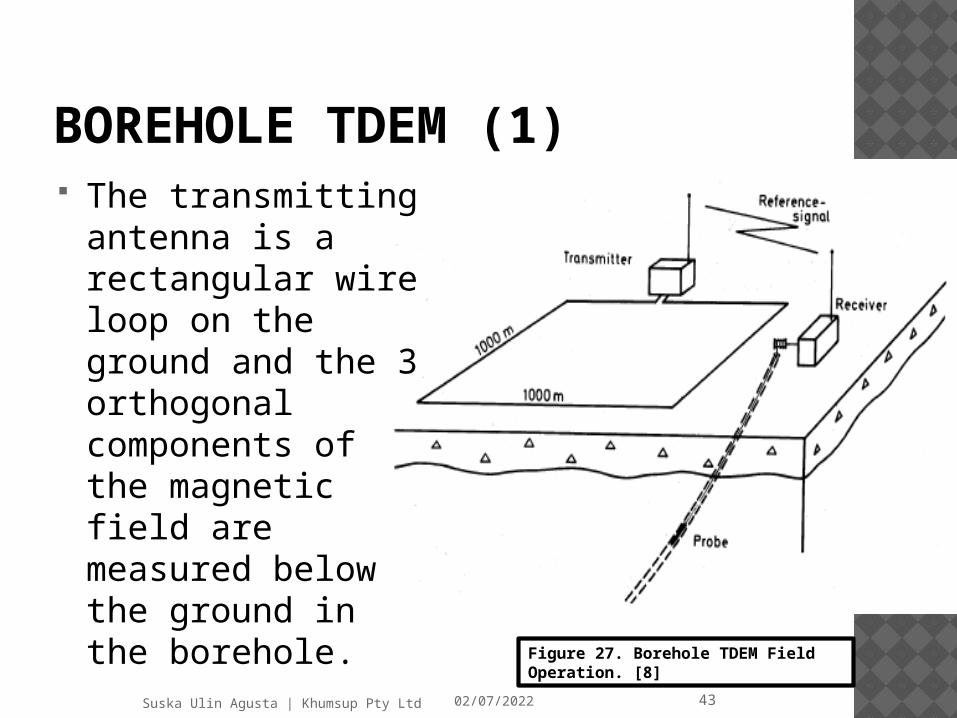
BOREHOLE TDEM (1) The transmitting

antenna is a rectangular wire loop on the ground and the 3 orthogonal components of the magnetic field are measured below the ground in the borehole.

Figure 27. Borehole TDEM Field Operation. [8]


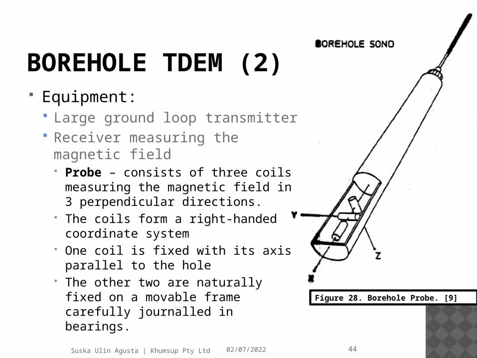
Equipment: Large ground loop transmitter Receiver measuring the magnetic

field Probe – consists of three coils

measuring the magnetic field in 3 perpendicular directions.

The coils form a right-handed coordinate system

One coil is fixed with its axis parallel to the hole

The other two are naturally fixed on a movable frame carefully journalled in bearings.

BOREHOLE TDEM (2)

Figure 28. Borehole Probe. [9]


REFERENCES1. Kearey, P., Brooks, M., Hill, Ian. 2002. An Introduction to Geophysical

Exploration. London : Blackwell Science Ltd.

2. Time-domain Electromagnetic Exploration. Northwest Geophysical Associates, Inc.

3. Lange, G., Seidel, K. Electromagnetic Methods. Environmental Geology, 4 Geophysics.

4. PROTEM TDEM Systems Brochure Specifications.

5. Sorensen, K. I., Christiansen. A. V., Auken, E. The Transient Electromagnetic Method. Burval.

6. Everett, M. E., Benavides, A., Pierce J. C. 2005. An experimental study of the time-domain electromagnetic response of a buried conductive plate. Geophysics VOL 70, NO.1.

7. Descloitres, M., Guerin, R., Albuoy, Y., Tabbagh, A., Ritz, M. 2000. Improvement in TDEM sounding interpretation in presence of IP. Journal of Applied Geophysics 45 (2000) 1-18.

8. Lecture 12 TDEM Methods. Applied and Environmental Geophysics.

9. Malmqvist, L., Pantze, R., Kristensson, G., Karlsson, A. 1990. Electromagnetic Fields in Boreholes – Measurements in 3D. Department of Electroscience Electromagnetic Theory Lund Institute of Technology Sweden.

tdem surveying

Documents