thomasc.mtcmlee/pdffiles/2002anzjs.pdf · dresses the denoising of noisy data using the bob method....

Aust. N. Z. J. Stat. 44(1), 2002, 23–39

TREE-BASED WAVELET REGRESSION FOR CORRELATED DATAUSING THE MINIMUM DESCRIPTION LENGTH PRINCIPLE

Thomas C.M. Lee1

Colorado State University

Summary

This paper considers the problem of non-parametric regression using wavelet techniques.Its main contribution is the proposal of a new wavelet estimation procedure for recoveringfunctions corrupted by correlated noise, although a similar procedure for independent noiseis also presented. Two special features of the proposed procedure are that it imposes a so-called ‘tree constraint’ on the wavelet coefficients and that it uses the minimum descriptionlength principle to define its ‘best’ estimate. The proposed procedure is empirically com-pared with some existing wavelet estimation procedures, for the cases of independent andcorrelated noise.

Key words: correlated noise; minimum description length principle; non-Gaussian noise; tree con-straint; wavelet regression.

1. Introduction

In recent years wavelet techniques for non-parametric regression have attracted enormousattention from researchers across different fields. Two main reasons for this are that waveletestimators enjoy excellent minimax properties and that they are capable of adapting to spatialand frequency inhomogeneities (see e.g. Donoho & Johnstone, 1994, 1995; Donoho et al.,1995). Also, they are backed up by a fast algorithm (see e.g. Mallat, 1989).

Most existing wavelet-based non-parametric regression methods were designed for re-covering data corrupted by independent Gaussian noise. The primary goal of this paper is topropose a wavelet function estimation procedure that is capable of handling correlated data.Two characteristics of this procedure are that it imposes a so-called ‘tree constraint’on the classof all plausible function estimates and that the final function estimate is chosen by the mini-mum description length (MDL) principle (see Rissanen, 1989 Chapter 3, and references giventherein). Of course, the proposed procedure also handles independent noise; furthermore, itcan be made specialized to handle non-Gaussian noise (see Section 6.1).

This paper is arranged as follows. Section 2 provides background material for waveletregression. Section 3 describes how the MDL principle can be applied to the problem of

Received April 1999; revised September 2000; accepted October 2000.∗Author to whom correspondence should be addressed.1 Dept of Statistics, Colorado State University, Fort Collins, CO 80523-1877, USA.

e-mail: [email protected]. The author thanks Victor Solo for many discussions, Michael Stein for many constructivecomments and an insightful discussion which led to the idea of tree representation, Kenneth Wilder for dis-cussions on classification trees, and Fanis Sapatinas and Bernard Silverman for providing their BUTHRESHroutines. The author also thanks the referees and the associate editor for many useful comments and ques-tions which have led to this substantially improved version of the paper. Numerical work was done using thewavethresh package of Nason & Silverman (1994). S-PLUS® codes for the SURE procedure were adoptedfrom Luo & Wahba (1997).

c© Australian Statistical Publishing Association Inc. 2002. Published by Blackwell Publishing Ltd.

24 THOMAS C.M. LEE

wavelet regression. Section 4 presents an existing MDL criterion (due to Saito). In Section 5,we show that, to some extent, Saito’s criterion can be simplified by imposing a tree constrainton the wavelet coefficients. Section 6 presents the proposed procedure. Section 7 reportssimulation results and Section 8 draws conclusions.

While this paper was being revised, the author became aware of the closely related workby Moulin (1996), in which an MDL tree-based wavelet regression procedure is proposed.However, Moulin (1996) does not handle correlated noise or provide any simulation resultsregarding the practical performance of the procedure.

2. Background: wavelet regression

Suppose we observe n equidistant noisy observations:

yi = fi + ei, fi = f( i

n − 1

)(i = 0, . . . , n − 1) ,

where f is an unknown function, and the ei are noise. Our goal is to recover f using waveletmethods. For simplicity, we assume that n = 2J+1 is an integer power of 2, and considerboth independent and correlated noise.

Broadly speaking, wavelet methods for non-parametric regression involve two steps. Thefirst step is to obtain the empirical wavelet coefficient vector w by applying a discrete wavelettransform (DWT) to the observations y = (y0, . . . , yn−1). If we denote the DWT matrix byW (see e.g. Donoho & Johnstone, 1994), w is given by w = Wy. Here w is an n× 1 vectorand we follow Donoho & Johnstone (1994) and use a double indexing scheme to label itselements:

w = (w−1,0︸︷︷︸,︷︸︸︷w0,0, w1,0, w1,1︸︷︷︸,

︷︸︸︷w2,0, w2,1, w2,2, w2,3, . . . , wj,k, . . . , wJ,0, . . . , wJ,2J −1︸︷︷︸) .

Therefore, with the exception of the first element, the indexing scheme is: wj,k , j = 0, . . . , J ;k = 0, . . . , 2J − 1.

The second step is to apply a filtering operation (e.g. thresholding) to w and obtain anestimated wavelet coefficient vector w. Then an estimate f of f = (f0, . . . , fn−1) can be

obtained by applying the inverse DWT to w: f = W Tw. Below we describe three types offiltering operation: thresholding, recursive partitioning and methods based on hidden Markovmodels.

2.1. Thresholding

Thesholding is perhaps the most widely studied filtering operation; it is widely knownthat the quality of f is highly dependent on the threshold values. For the case of independentnoise, various automatic methods have been proposed for choosing their values. These meth-ods include the ‘universal’ thresholding scheme of Donoho & Johnstone (1994), the SUREthresholding scheme of Donoho & Johnstone (1995), the cross-validation scheme of Nason(1996) and the cross-validatory AIC scheme of Hurvich & Tsai (1998). Bayesian methodshave also been proposed: see Chipman, Kolaczyk & McCulloch (1997), Abramovich, Sap-atinas & Silverman (1998) and Vidakovic (1998). Of particular interest to the present paperis the MDL-based scheme proposed by Saito (1994). This MDL-based scheme was furtherstudied by Antoniadis, Gijbels & Gregoire (1997) and it is discussed in detail in Section 4.

c© Australian Statistical Publishing Association Inc. 2002

TREE-BASED WAVELET REGRESSION FOR CORRELATED DATA 25

Correlated noise has also been considered (although to a much smaller extent). Wang(1996) provides some asymptotic minimax results, and modifies the independent noise ‘uni-versal’ and cross-validation thresholding schemes so that they can be applied to correlateddata. Johnstone & Silverman (1997) demonstrate that, even though the SURE thresholdingscheme of Donoho & Johnstone (1995) was originally designed for independent noise, it isalso applicable for correlated data. They also establish many theoretical minimax results. An-other proposal for dealing with correlated noise is described in Solo (1998). His approach isto define the estimate f as the minimizer of an L1-penalized weighted least squares criterion.Because the minimization of such a criterion is not trivial, a minimization algorithm, modifiedfrom the CLEAN algorithm of radiophysics, was developed.

2.2. Recursive partitioning

Engel (1994) provides another example of a filtering operation for handling independentdata. His procedure is specialized to the Haar wavelet system, and is closely related to theCART method developed by Breiman et al. (1984). The idea behind it is to approximate thetrue function by a piecewise constant function and use a recursive partitioning scheme to finda ‘best-fit’piecewise constant function. Note that in similar situations, a recursive partitioningscheme can usually be treated as some sort of tree-growing or pruning algorithm.

Donoho (1997) discusses a connection between the CART method for non-parametricregression and the BOB (best-ortho-basis) method for time-frequency analysis. He also ad-dresses the denoising of noisy data using the BOB method. However, he does not discuss theissue of correlated data.

2.3. Hidden Markov models

Crouse, Nowak & Baraniuk (1998) introduced a novel wavelet regression procedure thatuses hidden Markov models. Their procedure was designed for independent noise, and can bedescribed as follows. Each wavelet coefficient is associated with a hidden binary state variableS; the value of S is unobservable. If S = 0, say, the corresponding wavelet coefficient is‘suspected’ to be a ‘noise coefficient’, and is treated as a realization of a zero-mean Gaussiandensity with a small variance σ 2

S . On the other hand, if S = 1, say, the correspondingwavelet coefficient is ‘suspected’ to be a ‘signal coefficient’, and is treated as a realization ofa zero-mean Gaussian density with a high variance σ 2

H . Both σ 2S and σ 2

H are unknown.Then the dependencies of the state variables are modelled by a probabilistic graph with

a tree structure. Note that this is different from imposing a tree dependency structure directlyon the wavelet coefficients (which is the approach taken by the present paper). The nextstep is to apply an EM algorithm to obtain the maximum likelihood estimates of the hiddenstate probabilities, σ 2

S and σ 2H . Once these estimates are computed, final wavelet coefficient

estimates are obtained by an empirical Bayesian procedure.

3. MDL for wavelet regression

We motivate our discussion of the MDL principle by the following problem. Supposea set of observed data z and a class of plausible models � = {θ1, . . . , θm} for z are given,and our goal is to select a ‘best’ model for z from �. It is allowed that different θi mayhave different numbers of parameters. One typical example is subset selection in the multipleregression context.


26 THOMAS C.M. LEE

The MDL principle provides a powerful method for attacking such model selection prob-lems. In short, the MDL principle defines the ‘best’ model as the one that enables the bestencoding (or compression) of the data z, so that z can be transmitted in the most economicalway. That is, the best fitted model is the one that produces the shortest codelength of z. Inthe present context, the codelength of z can be treated as the amount of memory space that isrequired to store z.

One general method for encoding z is to ‘split’ z into two components: a fitted model θ

plus the corresponding residuals r. Rissanen (1989 pp. 54–58) called this ‘two-part coding’.We follow Rissanen’s notation and use L(a) to denote the codelength for the object a. Wehave

L(z) = L(θ) + L(r | θ) .

The MDL principle defines the best θ as the one that gives the smallest L(z). In the aboveexpression we have stressed that r is ‘conditional’ on θ .

For the wavelet regression problem that we consider here, z corresponds to y, θ corre-sponds to f or w (note that there is a one-to-one correspondence between f and w), andr corresponds to e = y − f . In other words, the MDL principle suggests that w should bechosen as the one that minimizes

L(y) = L(w) + L(e | w) . (1)

Thus to apply the MDL principle to the problem of wavelet regression, we must first derive anexpression for L(y), and then develop a procedure for minimizing the derived expression.

4. An existing MDL criterion for independent noise

When the noise is independent, Saito (1994) developed an MDL-based procedure for ob-taining w (and hence f ). His procedure keeps the first m largest (in terms of absolute value)wavelet coefficients and deletes all the remaining ones, where m is chosen as the minimizer ofan MDL criterion that he derived (i.e. an expression for L(y)). Thus his procedure is equivalentto a global thresholding scheme that has its threshold value chosen as any number between themth and (m + 1)th largest absolute values of the empirical wavelet coefficients. Antoniadiset al. (1997) provide supportive theoretical and simulation results for Saito’s criterion.

To encode w so that it can be transmitted, we need to encode (i) the indices, and (ii) theactual estimated values of those non-zero coefficients wjk in w. Since the index of a non-zerocoefficient wjk is an integer between 1 and n, Saito asserts that the codelength for encodingsuch an index is log2 n. For the codelength of encoding the actual values of those estimatednon-zero coefficients in w, we can apply the result of Rissanen (1989 pp .55–56), which saysthe codelength for encoding one of these estimated values is 1

2 log2 n. One heuristic argumentfor this result is as follows. Each wjk is estimated from n noisy observations, so there is noneed to encode wjk to a precision that is finer than its standard error. Now as the standard error

is asymptotically of order√

n, it suggests that wjk can be effectively encoded with 12 log2 n

bits. Thus, if there are m non-zero coefficients in w, the total codelength for encoding w is

L(w) = L(‘indices’) + L(‘actual estimated values’)

= m log2 n + 12 m log2 n = 3

2 m log2 n . (2)



Now if an estimated w is ‘reasonable’, the residual e approximately satisfies the modelassumption (independent Gaussian for the current situation). Rissanen (1989 pp .54–55)shows that, by using this fact, the codelength L(e | w) for encoding e is given by the nega-tive of the conditional log-likelihood (base 2) of e given w. When the noise is independentGaussian and if we estimate σ 2 by σ 2 = ‖e‖2/n, this negative conditional log-likelihoodbecomes (‖x‖2 is defined as xTx)

− log2

{( 1√2πσ 2

)n

exp(

− ‖e‖2

σ 2

)}= 1

2n log2 2π + 12n log2

‖e‖2

n+ n .

Thus, for minimization purposes, we can take

L(e | w) = 12n log2

‖e‖2

n. (3)

Therefore, combining (1), (2) and (3), we have Saito’s criterion

LS(y) = L(w) + L(e | w) = 32 m log2 n + 1

2n log2‖e‖2

n. (4)

However, in cases where the non-zero wavelet coefficients ‘cluster’ together, we claimthat there is redundancy in Saito’s criterion. By ‘cluster’ we mean that if wjk is non-zerothen wj−1,k , wj,k−1 , wj,k+1 and wj+1,k are also non-zero. Thus, when encoding such aw, we can make use of this fact and obtain a smaller value for L(w) (i.e. with a shortercodelength expression for w). This means that, in cases where ‘clustering’ is present (asdefined previously), Saito’s criterion over-penalizes the number of non-zero coefficients andhence has a tendency to underestimate the ‘true’ m.

5. Tree constraint

How can a w be encoded so that the above ‘clustering’property is captured? One possibleapproach is to use a tree to represent the indices of the non-zero elements of w. As we shallsee later, another advantage of using a tree representation is that it agrees with the intuitionthat wavelet coefficients at a finer level (or resolution) should have a greater chance of beingdeleted than those coarser level wavelet coefficients at the same relative location. The firstelement w−1,0 of a w carries the information of the mean of y, so it should always be kept(unless y is a zero-mean white noise). For this reason, we ignore the index of w−1,0 andfocus on the indices of the remaining non-zero elements of a w.

Define wj+1,2k and wj+1,2k+1 as the ‘children’ of wjk, 0 ≤ j < J. We also call wjk

the ‘parent’ of wj+1,2k and wj+1,2k+1. We impose the constraint that, if wjk is deleted, noneof its children can survive. That is, for 0 ≤ j < J,

wjk = 0 ⇒ wj+1,2k = 0 and wj+1,2k+1 = 0 .

This sort of constraint, sometimes known as tree constraint, is just a severe executioner of theintuition mentioned above that wavelet coefficients at finer levels should have higher chancesof being deleted.

Once tree constraint is imposed, the idea of tree representation is straightforward. Weillustrate it with an example. Suppose the only non-zero elements of w are w00 , w10 , w11 ,


28 THOMAS C.M. LEE

w

w w

w

w

w w

00

10 11

20 22 23

31w w30 35

Figure 1. An example illustrating the tree representation of the indices of non-zero coefficients in w

L(2)

T(1)

N(4) N(5)

R(7)

N(8)

N(9)T(3)

T(6)

Figure 2. Node attributes and traversal order (in parenthesis) of the tree displayed in Figure 1

w20 , w22 , w23 , w30 , w31 and w35 . The indices, or the relative positions, of these elementscan be represented by the tree shown in Figure 1. Note that w10 and w22 have only one child.

By imposing tree-constraint on wavelet coefficients we can capture the ‘clustering’ prop-erty as defined previously. However, it is known that large coefficients do not always ‘cluster’together, especially from one resolution level to another (i.e. from j to j + 1). Indeed, it istrue only along a sub-sequence of the resolution levels (see Daubechies, 1992 p .300). There-fore, by imposing tree constraint we might delete large wavelet coefficients at high resolutionlevel and induce numerical errors even without noise. Of course, there are cases where thosenumerical errors are smaller than the error due to noise and in such cases the proposed methodis acceptable. Section 7.1 provides some examples.

The next task is to construct a method for encoding the tree structure. Various methodsfor encoding and optimizing classification trees are proposed in the literature; see e.g. Quinlan& Rivest (1989), Wallace & Patrick (1993) and Rissanen (1997). However, these methods arenot suitable for our purposes because they all assume that all internal nodes of a classificationtree have two children. Note also that the tree structure implicitly defined by the waveletrecursive partitioning scheme of Engel (1994) also falls into this category.

Here we suggest a tree-encoding method which allows for the possibility that an internalnode possesses only one child. First notice that a node can only have one of the followingfour attributes: possesses no children (N), possesses a left child (L), possesses a right child(R) and possesses two children (T). Thus, if we agree to traverse a tree in a recursive, top-down, depth-first and left-first manner, we can encode the tree structure by just encoding theattributes of its nodes in the order that the nodes are visited.

To illustrate the idea, the tree in Figure 1 is re-drawn in Figure 2 with node attributes andtraversal order displayed. Therefore, by using the above traversal scheme, the tree structureis represented by ‘TLTNNTRNN’.



6. A tree-based MDL criterion

We present a new MDL criterion using a tree constraint on wavelet coefficients. First, weassume that the noise is independent and then we explain how to handle the case of correlatednoise. We also briefly describe a tree-growing strategy for (approximately) minimizing thisnew criterion.

6.1. Independent noise

Recall that an MDL criterion, or codelength expression, for wavelet regression is ofthe form L(y) = L(w) + L(e | w), and L(w) can be further decomposed into L(w) =L(‘indices’) + L(‘actual estimated values’); see (2). What is L(‘indices’) when the indicesare represented by a tree?

There are only four possible attributes for each node of a tree. Thus log2 4 = 2 bitsare needed to encode the attribute of one node. If there are m non-zero wavelet coefficients(i.e. m nodes), L(‘indices’) = 2m and hence L(w) = 2m + 1

2 m log2 n; see (2). Using theslightly vague argument that because n is usually large and m is small and thus the term 2m

is negligible, we approximate L(w) by L(w) ≈ 12 m log2 n .

If the noise is independent Gaussian, combining (1), L(w) ≈ 12 m log2 n and (3), L(y)

can be approximated by

MDLIND(f ) = 12 m log2 n + 1

2n log2‖e‖2

n. (5)

When the noise is known to be independent Gaussian, we propose that f can be estimatedby the minimizer of MDLIND(f ), subject to the condition that the tree constraint is satisfied.

The criterion MDLIND(f ) can be modified for handling non-Gaussian noise if the densityfunction of the noise, say g, is known up to a dispersion parameter φ. The second term ofMDLIND(f ) is the codelength for encoding the residual e and it is given by the negative ofthe conditional log-likelihood of e given w. Thus a modified criterion for non-Gaussian noisecan be obtained by replacing the second term in MDLIND(f ) by − log2 g(e | w). Previouswork on non-Gaussian noise can be found, for example, in Moulin (1994), Neumann & vonSachs (1995) and Gao (1997).

6.2. Correlated noise

Suppose that the noise ei is correlated, and can be adequately modelled by an autore-gressive (AR) series of an unknown order p:

ei = a1ei−1 + a2ei−2 + · · · + apei−p + τi ,

where a = {a1, . . . , ap} are unknown AR parameters and τi is a Gaussian innovation. Thisreduces to the independent noise case when p = 0. Extension to autoregressive moving-average (ARMA) noise or even autoregressive integrated moving-average (ARIMA) noise isconceptually simple, but for computational reasons we do not pursue it here.

Under the autoregressive dependence, the codelength expression L(e | w) can be decom-posed into

L(e | w) = L(a | w) + L(τ | a, w) ,


30 THOMAS C.M. LEE

where a is an estimate of a, τ = (τ1, . . . , τn) with τi = ei − a1ei−1 −· · ·− ap ei−p , and p isan estimate of p. Now as each of a1, a2, . . . , ap is estimated from n data points, L(a | w) ≈12 p log2 n (see the heuristic argument given in the second paragraph of Section 4). Also, ifw and a are reasonable estimates, then, by model assumption, τ would be (approximately)independent normal, and hence L(τ | a, w) ≈ 1

2n log2(‖τ‖2/n) (similar to (3)). Thereforewe have

L(e | w) = L(a | w) + L(τ | a, w) ≈ 12 p log2 n + 1

2n log2‖τ‖2

n.

The ei can be treated as an AR series, and the above codelength expression agrees with theclassical one discussed for example in Hannan & Quinn (1979).

Using steps similar to those in Section 6.1, we obtain the following criterion, which canbe taken as an approximation for L(y) when the noise is autoregressively correlated:

MDLCOR(f ) = 12 (m + p) log2 n + 1

2n log2‖τ‖2

n. (6)

When the noise is correlated, we propose that f can be estimated by the minimizer of thecriterion MDLCOR(f ), subject to the tree constraint.

Observe that MDLCOR(f ) is a generalization of MDLIND(f ), as MDLCOR(f ) reducesto MDLIND(f ) when p = 0. For this reason, if it is not clear whether the noise is indepen-dent or correlated, we recommend using MDLCOR(f ) as the target. In fact, in the numericalexperiments reported in Section 7, we always use MDLCOR(f ) as our target even when thenoise is independent.

6.3. Tree-growing

The imposition of the tree constraint suggests a natural tree-growing algorithm for ap-proximating the minimizer of MDLIND(f ) (or MDLCOR(f )). The idea is straightforward:the root node (w00) is the initial tree, and at each time-step the tree grows by the addition ofa best-embryo node. An embryo node is a node which is directly linked but does not belongto the current tree, and a best-embryo node is defined as the embryo node that has the largestabsolute value amongst all other embryo nodes. (A best-embryo node can also be defined in adifferent way. For example, a best embryo node can be defined as the embryo node such that,when it is added to the current tree, it gives the largest reduction in the value of MDLIND(f )

or MDLCOR(f ).)

The tree-growing algorithm continues until the size, in terms of number of nodes, of thetree hits a pre-set limit SMAX (a maximal tree is of size n − 1). Thus, when the algorithmfinishes, a nested sequence of SMAX trees is produced, and the tree that gives the smallestvalue of MDLIND(f ) or MDLCOR(f ) is taken as the final estimate. When we are searchingfor the minimizer of MDLCOR(f ), an additional step for searching for a ‘best’ AR order isrequired, and that a maximal AR searching order pMAX has to be imposed. Also, we maywant to impose a minimum size limit SMIN for the final chosen tree, recognising that, in someexisting wavelet thresholding schemes, low level wavelet coefficients are not thresholded.Throughout our numerical experiments we set SMAX = 1

2n, SMIN = 0 and pMAX = 4.



Blocks

0.0 0.2 0.4 0.6 0.8 1.0

-20

24

6

Doppler

0.0 0.2 0.4 0.6 0.8 1.0-0.6

-0.4

-0.2

0.0

0.2

0.4

0.6

Heavisine

0.0 0.2 0.4 0.6 0.8 1.0

-6-4

-20

24

Bumps

0.0 0.2 0.4 0.6 0.8 1.0

01

23

4

BrokenPoly

0.0 0.2 0.4 0.6 0.8 1.0

0.0

0.2

0.4

0.6

0.8

1.0

Figure 3. Plots of test functions

Saito’s criterion (4) can, in principle, be extended to handle correlated noise, just as weextended criterion (5) to (6). However, the minimization of such a modified Saito’s criterionmay not be practically feasible, as the tree-growing algorithm can no longer be applied.

7. Numerical experiments

This section reports results of three numerical experiments. We used five test func-tions: the four test functions Blocks, Doppler, Heavisine and Bumps of Donoho & Johnstone(1994), and the broken polynomial test function (which we call BrokenPoly) of Nason &Silverman (1994). These five test functions are plotted in Figure 3. Also, throughout the threeexperiments, we used Daubechies’s order 4 ‘least asymmetric’ wavelet (Daubechies, 1992pp. 198–199). For evaluating the quality of an estimated f , we used the numerical measureMISE(f ) = ‖f − f ‖2, which was taken as an approximation of the mean integrated squarederror.

7.1. No noise

To investigate the possibility that imposing the tree constraint may prevent a true func-tion from being completely recovered, we applied our tree-growing algorithm for minimizingMDLCOR(f ) to recover the testing functions using the functions themselves as the observeddata. That is, no noise was present. The recovered functions are virtually identical to thetrue functions, except for some numerical errors: the values of log MISE(f ) for the five testfunctions are −46.82, −18.92, −23.06, −12.90 and −50.77, respectively. These valuesare much smaller than the corresponding values of log MISE(f ) reported below.

7.2. Independent noise

In this subsection we investigate the relative practical performances of four wavelet re-gression methods when the noise is independent:

1. the SURE thresholding procedure of Donoho & Johnstone (1995);2. the Bayesian thresholding procedure of Abramovich et al. (1998);3. the MDL-based thresholding (MDL-Thresh) procedure of Saito (1994); and4. the proposed tree-growing procedure (MDL-Tree) which aims to minimize MDLCOR(f )

(rather than MDLIND(f )).

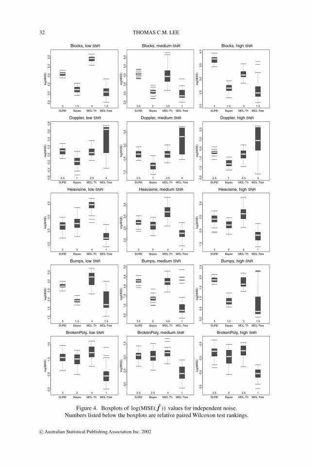
We defined the signal-to-noise ratio (SNR) as SNR = ‖f ‖/σ (as in Donoho & Johnstone,1994), and used three levels: high SNR = 9, medium SNR = 7 and low SNR = 5. For eachcombination of test function and SNR, 50 sets of noisy observations were simulated, and thenumber of data points n for each dataset was 512.

For each simulated dataset, we applied the four wavelet methods listed above to estimatethe test function. For each combination of test function and SNR, Figure 4 displays boxplots


32 THOMAS C.M. LEE

3.0

3.5

4.0

4.5

5.0

5.5

SURE Bayes MDL-Th MDL-Tree

Blocks, low SNRlo

g(M

ISE

)

3 1.5 4 1.5

2.5

3.0

3.5

4.0

4.5

5.0


Blocks, medium SNR

log(

MIS

E)

3.5 2 3.5 1 2.0

2.5

3.0

3.5

4.0


Blocks, high SNR

log(

MIS

E)

4 1.5 3 1.5

-0.6

-0.4

-0.2

0.0

0.2

0.4

0.6

0.8


Doppler, low SNR

log(

MIS

E)

2.5 1 2.5 4

-1.0

-0.5

0.0

0.5


Doppler, medium SNRlo

g(M

ISE

)

2.5 1 2.5 4 -2.0

-1.5

-1.0

-0.5

0.0

0.5


Doppler, high SNR

log(

MIS

E)

2.5 1 2.5 4

2.5

3.0

3.5

4.0


Heavisine, low SNR

log(

MIS

E)

2 3 4 1

2.0

2.5

3.0

3.5


Heavisine, medium SNR

log(

MIS

E)

3 2 4 1

1.5

2.0

2.5

3.0


Heavisine, high SNR

log(

MIS

E)

3 2 4 1

1.0

1.5

2.0

2.5

3.0

3.5


Bumps, low SNR

log(

MIS

E)

3 1.5 4 1.5

0.5

1.0

1.5

2.0

2.5

3.0


Bumps, medium SNR

log(

MIS

E)

3.5 2 3.5 1 0.0

0.5

1.0

1.5

2.0

2.5


Bumps, high SNR

log(

MIS

E)

4 1.5 3 1.5

-2.5

-2.0

-1.5

-1.0


BrokenPoly, low SNR

log(

MIS

E)

3 2 4 1

-3.0

-2.5

-2.0

-1.5


BrokenPoly, medium SNR

log(

MIS

E)

2.5 2.5 4 1

-3.5

-3.0

-2.5

-2.0


BrokenPoly, high SNR

log(

MIS

E)

3.5 2 3.5 1

Figure 4. Boxplots of log(MISE(f )) values for independent noise.Numbers listed below the boxplots are relative paired Wilcoxon test rankings.



noisy data

0.0 0.2 0.4 0.6 0.8 1.0

-20

24

6

SURE

MISE= 53.7530.0 0.2 0.4 0.6 0.8 1.0

-20

24

6

MDL-Thresh

MISE= 55.7360.0 0.2 0.4 0.6 0.8 1.0

-20

24

6

Bayes

MISE= 26.0180.0 0.2 0.4 0.6 0.8 1.0

-20

24

6

MDL-Tree

MISE= 17.4750.0 0.2 0.4 0.6 0.8 1.0

-20

24

6

noisy data

0.0 0.2 0.4 0.6 0.8 1.0-0.6

-0.4

-0.2

0.0

0.2

0.4

0.6

SURE

MISE= 0.828540.0 0.2 0.4 0.6 0.8 1.0-0

.6-0

.4-0

.20.

00.

20.

40.

6

MDL-Thresh

MISE= 0.898710.0 0.2 0.4 0.6 0.8 1.0-0

.6-0

.4-0

.20.

00.

20.

40.

6

Bayes

MISE= 0.519750.0 0.2 0.4 0.6 0.8 1.0-0

.6-0

.4-0

.20.

00.

20.

40.

6

MDL-Tree

MISE= 1.03630.0 0.2 0.4 0.6 0.8 1.0-0

.6-0

.4-0

.20.

00.

20.

40.

6

noisy data

0.0 0.2 0.4 0.6 0.8 1.0

-6-4

-20

24

SURE

MISE= 13.9110.0 0.2 0.4 0.6 0.8 1.0

-6-4

-20

24

MDL-Thresh

MISE= 27.8260.0 0.2 0.4 0.6 0.8 1.0

-6-4

-20

24

Bayes

MISE= 19.3310.0 0.2 0.4 0.6 0.8 1.0

-6-4

-20

24

MDL-Tree

MISE= 9.93380.0 0.2 0.4 0.6 0.8 1.0

-6-4

-20

24

noisy data

0.0 0.2 0.4 0.6 0.8 1.0

01

23

4

SURE

MISE= 10.9850.0 0.2 0.4 0.6 0.8 1.0

01

23

4

MDL-Thresh

MISE= 10.0840.0 0.2 0.4 0.6 0.8 1.0

01

23

4

Bayes

MISE= 4.14540.0 0.2 0.4 0.6 0.8 1.0

01

23

4MDL-Tree

MISE= 2.12770.0 0.2 0.4 0.6 0.8 1.0

01

23

4noisy data

0.0 0.2 0.4 0.6 0.8 1.0

0.0

0.2

0.4

0.6

0.8

1.0

SURE

MISE= 0.14870.0 0.2 0.4 0.6 0.8 1.0

0.0

0.2

0.4

0.6

0.8

1.0

MDL-Thresh

MISE= 0.107260.0 0.2 0.4 0.6 0.8 1.0

0.0

0.2

0.4

0.6

0.8

1.0

Bayes

MISE= 0.108450.0 0.2 0.4 0.6 0.8 1.0

0.0

0.2

0.4

0.6

0.8

1.0

MDL-Tree

MISE= 0.0746840.0 0.2 0.4 0.6 0.8 1.0

0.0

0.2

0.4

0.6

0.8

1.0

Figure 5. Estimates of the five test functions obtained fromindependent noisy observations, medium SNR

of the values of log MISE(f ) (for all f ). We also performed paired Wilcoxon tests to test ifthe difference between the median MISE(f ) values of two wavelet methods was significantor not. The significance level used was 1.25%, and the relative rankings, with 1 being thebest, are also listed below the corresponding boxplots in Figure 4. Ranking the methods inthis manner is not perfectly legitimate, but it provides an indicator of the relative merits of themethods (see Wand, 2000).

To visually evaluate and compare the performances of the four wavelet regression meth-ods, we did the following. For the combination of the test function Blocks and medium SNR,we ranked the 50 f s obtained by the proposed tree-based method, according to their values ofMISE(f ). The 25th best f , together with the corresponding simulated noisy data, is plottedin Figure 5. Estimates obtained by applying the other three wavelet regression methods to thissame simulated noisy dataset are also plotted in Figure 5. The same procedure was repeatedfor the remaining four test functions, and the results are also displayed in Figure 5.


34 THOMAS C.M. LEE

12

34

SURE MDL-Tree

Blocks, AR(1)

log(

MIS

E)

2 1

2.0

2.5

3.0

3.5

SURE MDL-Tree

Blocks, AR(2)

log(

MIS

E)

1.5 1.5 2.6

2.8

3.0

3.2

3.4

3.6

3.8

4.0

SURE MDL-Tree

Blocks, ARMA(1,1)

log(

MIS

E)

2 1

-2.0

-1.5

-1.0

-0.5

0.0

0.5

SURE MDL-Tree

Doppler, AR(1)

log(

MIS

E)

2 1

-1.5

-1.0

-0.5

0.0

0.5

SURE MDL-Tree

Doppler, AR(2)

log(

MIS

E)

1 2

-1.5

-1.0

-0.5

0.0

0.5

SURE MDL-Tree

Doppler, ARMA(1,1)

log(

MIS

E)

1 2

01

23

SURE MDL-Tree

Heavisine, AR(1)

log(

MIS

E)

2 1

12

3

SURE MDL-Tree

Heavisine, AR(2)

log(

MIS

E)

2 1

2.0

2.5

3.0

SURE MDL-Tree

Heavisine, ARMA(1,1)lo

g(M

ISE

)

1.5 1.5

12

3

SURE MDL-Tree

Bumps, AR(1)

log(

MIS

E)

2 1

1.5

2.0

2.5

SURE MDL-Tree

Bumps, AR(2)

log(

MIS

E)

2 1

1.5

2.0

2.5

3.0

3.5

SURE MDL-Tree

Bumps, ARMA(1,1)

log(

MIS

E)

1.5 1.5

-5-4

-3-2

SURE MDL-Tree

BrokenPoly, AR(1)

log(

MIS

E)

2 1

-4-3

-2-1

SURE MDL-Tree

BrokenPoly, AR(2)

log(

MIS

E)

2 1 -3.0

-2.5

-2.0

-1.5

SURE MDL-Tree

BrokenPoly, ARMA(1,1)

log(

MIS

E)

2 1

Figure 6. Boxplots of log(MISE(f )) values for correlated noise.Numbers listed below the boxplots are relative paired Wilcoxon test rankings.



noisy Blocks, AR(1)

0.0 0.2 0.4 0.6 0.8 1.0

-20

24

SURE estimate

MISE= 14.4320.0 0.2 0.4 0.6 0.8 1.0

-20

24

MDL-Tree estimate

MISE= 8.07940.0 0.2 0.4 0.6 0.8 1.0

-20

24

noisy Doppler, AR(1)

0.0 0.2 0.4 0.6 0.8 1.0

-0.4

-0.2

0.0

0.2

0.4

SURE estimate

MISE= 0.578390.0 0.2 0.4 0.6 0.8 1.0

-0.4

-0.2

0.0

0.2

0.4

MDL-Tree estimate

MISE= 0.506390.0 0.2 0.4 0.6 0.8 1.0

-0.4

-0.2

0.0

0.2

0.4

noisy Heavisine, AR(1)

0.0 0.2 0.4 0.6 0.8 1.0

-6-4

-20

24

SURE estimate

MISE= 14.2530.0 0.2 0.4 0.6 0.8 1.0

-6-4

-20

24

MDL-Tree estimate

MISE= 1.680.0 0.2 0.4 0.6 0.8 1.0

-6-4

-20

24

noisy Bumps, AR(1)

0.0 0.2 0.4 0.6 0.8 1.0

01

23

4

SURE estimate

MISE= 10.3270.0 0.2 0.4 0.6 0.8 1.0

01

23

4

MDL-Tree estimate

MISE= 3.11790.0 0.2 0.4 0.6 0.8 1.0

01

23

4

noisy BrokenPoly, AR(1)

0.0 0.2 0.4 0.6 0.8 1.0

0.0

0.2

0.4

0.6

0.8

1.0

SURE estimate

MISE= 0.10270.0 0.2 0.4 0.6 0.8 1.0

0.0

0.2

0.4

0.6

0.8

1.0

MDL-Tree estimate

MISE= 0.0164380.0 0.2 0.4 0.6 0.8 1.0

0.0

0.2

0.4

0.6

0.8

1.0

Figure 7. SURE and MDL-Tree estimates obtained from AR(1) correlated noisy observations


36 THOMAS C.M. LEE

noisy Blocks, AR(2)

0.0 0.2 0.4 0.6 0.8 1.0

-20

24

6SURE estimate

MISE= 25.3920.0 0.2 0.4 0.6 0.8 1.0

-20

24

6

MDL-Tree estimate

MISE= 18.8080.0 0.2 0.4 0.6 0.8 1.0

-20

24

6

noisy Doppler, AR(2)

0.0 0.2 0.4 0.6 0.8 1.0

-0.4

-0.2

0.0

0.2

0.4

SURE estimate

MISE= 0.374710.0 0.2 0.4 0.6 0.8 1.0

-0.4

-0.2

0.0

0.2

0.4

MDL-Tree estimate

MISE= 0.878030.0 0.2 0.4 0.6 0.8 1.0

-0.4

-0.2

0.0

0.2

0.4

noisy Heavisine, AR(2)

0.0 0.2 0.4 0.6 0.8 1.0

-6-4

-20

24

SURE estimate

MISE= 50.6380.0 0.2 0.4 0.6 0.8 1.0

-6-4

-20

24

MDL-Tree estimate

MISE= 7.07250.0 0.2 0.4 0.6 0.8 1.0

-6-4

-20

24

noisy Bumps, AR(2)

0.0 0.2 0.4 0.6 0.8 1.0

01

23

4

SURE estimate

MISE= 12.280.0 0.2 0.4 0.6 0.8 1.0

01

23

4

MDL-Tree estimate

MISE= 6.61790.0 0.2 0.4 0.6 0.8 1.0

01

23

4

noisy BrokenPoly, AR(2)

0.0 0.2 0.4 0.6 0.8 1.0

0.0

0.2

0.4

0.6

0.8

1.0

SURE estimate

MISE= 0.484790.0 0.2 0.4 0.6 0.8 1.0

0.0

0.2

0.4

0.6

0.8

1.0

MDL-Tree estimate

MISE= 0.0355910.0 0.2 0.4 0.6 0.8 1.0

0.0

0.2

0.4

0.6

0.8

1.0

Figure 8. Similar to Figure 7 except for AR(2) noise



noisy Blocks, ARMA(1,1)

0.0 0.2 0.4 0.6 0.8 1.0

-20

24

6SURE estimate

MISE= 24.70.0 0.2 0.4 0.6 0.8 1.0

-20

24

6

MDL-Tree estimate

MISE= 22.8250.0 0.2 0.4 0.6 0.8 1.0

-20

24

6

noisy Doppler, ARMA(1,1)

0.0 0.2 0.4 0.6 0.8 1.0

-0.4

-0.2

0.0

0.2

0.4

SURE estimate

MISE= 0.284510.0 0.2 0.4 0.6 0.8 1.0

-0.4

-0.2

0.0

0.2

0.4

MDL-Tree estimate

MISE= 0.774540.0 0.2 0.4 0.6 0.8 1.0

-0.4

-0.2

0.0

0.2

0.4

noisy Heavisine, ARMA(1,1)

0.0 0.2 0.4 0.6 0.8 1.0

-6-4

-20

24

SURE estimate

MISE= 40.4630.0 0.2 0.4 0.6 0.8 1.0

-6-4

-20

24

MDL-Tree estimate

MISE= 14.5030.0 0.2 0.4 0.6 0.8 1.0

-6-4

-20

24

noisy Bumps, ARMA(1,1)

0.0 0.2 0.4 0.6 0.8 1.0

01

23

4

SURE estimate

MISE= 7.62460.0 0.2 0.4 0.6 0.8 1.0

01

23

4

MDL-Tree estimate

MISE= 7.86060.0 0.2 0.4 0.6 0.8 1.0

01

23

4

noisy BrokenPoly, ARMA(1,1)

0.0 0.2 0.4 0.6 0.8 1.0

0.0

0.2

0.4

0.6

0.8

1.0

SURE estimate

MISE= 0.21450.0 0.2 0.4 0.6 0.8 1.0

0.0

0.2

0.4

0.6

0.8

1.0

MDL-Tree estimate

MISE= 0.099640.0 0.2 0.4 0.6 0.8 1.0

0.0

0.2

0.4

0.6

0.8

1.0

Figure 9. Similar to Figure 7 except for ARMA(1,1) noise


38 THOMAS C.M. LEE

Except for those cases associated with Doppler, the MDL-Tree procedure compares favour-ably with the other three procedures, although it also exhibits some instability, as the lengthof some MDL-Tree boxplots is relatively large.

7.3. Correlated noise

Here we are interested in the performances of the SURE procedure and the proposedMDL-Tree procedure (which aims to minimize MDLCOR(f )) when the noise is correlated.Johnstone & Silverman (1997) show that the SURE procedure is also applicable when thenoise is correlated.

The setup for this correlated noise experiment was essentially the same as for the inde-pendent noise experiment, with the exception that the noise e = (e1, . . . , en) was generatedfrom the ARMA(p, q) model

ei = a1ei−1 + · · · + apei−p + τi + b1τi−1 + · · · + bqτi−q ,

where τi denotes a Gaussian innovation. Three different types of ARMA noise were con-sidered: AR(1) with a1 = −0.8, AR(2) with a1 = 4/3 and a2 = −8/9, and ARMA (1,1)with a1 = 0.2 and b1 = −0.9. Throughout the whole experiment, the noise was alwayslinearly stretched so that (max(f ) − min(f ))/(max(e) − min(e)) = 5. Note that Johnstone& Silverman (1997) also use the same AR(2) noise in their numerical examples, and that theARMA(1,1) case does not satisfy the assumption made by MDLCOR(f ).

Boxplots, together with the corresponding paired Wilcoxon test rankings, are displayedin Figure 6, and the ‘25th best estimates’ are displayed in Figures 7–9. As before, except forDoppler, the MDL-Tree procedure compares favourably with the SURE procedure.

8. Conclusions

In this paper, a tree-based wavelet non-parametric regression procedure is proposed. Thisprocedure is designed to handle autoregressively correlated noise, and applies the MDL prin-ciple to choose its best estimate. Results of numerical experiments demonstrate that, exceptfor the cases of highly oscillating functions (e.g. Doppler), the proposed procedure providessatisfactory performances.

References

Abramovich, F., Sapatinas, T. & Silverman, B.W. (1998). Wavelet thresholding via a Bayesian approach.J. R. Stat. Soc. Ser. B Stat. Methodol. 60, 725–749.

Antoniadis, A., Gijbels, I. & Gregoire, G. (1997). Model selection using wavelet decomposition andapplications. Biometrika 84, 751–763.

Breiman, L., Friedman, J.H., Olshen, R.A. & Stone, C.J. (1984). Classification and Regression Trees.Belmont, CA: Wadsworth.

Chipman, H.A., Kolaczyk, E.D. & McCulloch, R.E. (1997). Adaptive Bayesian wavelet shrinkage.J. Amer. Statist. Assoc. 92, 1413–1421.

Crouse, M.S., Nowak, R.D. & Baraniuk, R.G. (1998). Wavelet-based statistical signal processing usinghidden Markov models. IEEE Trans. Signal Process. 46, 886–902.

Daubechies, I. (1992). Ten Lectures on Wavelets, Vol. 1. Philadelphia: Society for Industrial and AppliedMathematics.

Donoho, D.L. (1997). CART and best-ortho-basis: a connection.Ann. Statist. 25, 1870–1911.



Donoho, D.L. & Johnstone, I.M. (1994). Ideal spatial adaptation by wavelet shrinkage. Biometrika81, 425–455.

Donoho, D.L. & Johnstone, I.M. (1995). Adapting to unknown smoothness via wavelet shrinkage. J.Amer.Statist. Assoc. 90, 1200–1224.

Donoho, D.L., Johnstone, I.M., Kerkyacharian, G. & Picard, D. (1995). Wavelet shrinkage: asymp-topia? (With discussion). J. R. Stat. Soc. Ser. B Stat. Methodol. 57, 301–369.

Engel, J. (1994). A simple wavelet approach to nonparametric regression from recursive partitioning schemes.J. Multivariate Anal. 49, 242–254.

Gao, H-Y. (1997). Choice of thresholds for wavelet shrinkage estimate of the spectrum. J. Time Ser. Anal. 18,231–251.

Hannan, E.J. & Quinn, B.G. (1979). The determination of the order of an autoregression. J. R. Stat. Soc.Ser. B Stat. Methodol. 41, 190–195.

Hurvich, C.M.&Tsai, C-L. (1998).A crossvalidatoryAIC for hard wavelet thresholding in spatially adaptivefunction estimation. Biometrika 85, 701–710.

Johnstone, I.M. & Silverman, B.W. (1997). Wavelet threshold estimators for data with correlated noise.J. R. Stat. Soc. Ser. B Stat. Methodol. 59, 319–351.

Luo, Z. &Wahba, G. (1997). Hybrid adaptive splines. J. Amer. Statist. Assoc. 92, 107–116.Mallat, S.G. (1989). A theory for multiresolution signal decomposition: The wavelet representation. IEEE

Trans. Pattern Analysis and Machine Intelligence 11, 674–693.Moulin, P. (1994). Wavelet thresholding techniques for power spectrum estimation. IEEE Trans. Signal

Process. 42, 3126–3136.Moulin, P. (1996). Signal estimation using adapted tree-structured bases and the MDL principle. In Proc.

IEEE Signal Processing Symposium on Time-Frequency and Time-Scale Analysis, pp. 141–143. Paris.Nason, G.P. (1996). Wavelet shrinkage using cross-validation. J. R. Stat. Soc. Ser. B Stat. Methodol.

58, 463–479.Nason, G.P. & Silverman, B.W. (1994). The discrete wavelet transform. J. Comput. Graph. Statist. 3,

163–191.Neumann, M.H. & von Sachs, R. (1995). Wavelet thresholding: beyond the Gaussian i.i.d. situation. In

Wavelets and Statistics, eds A. Antoniadis & G. Oppenheim, pp. 301–330. New York: Springer-Verlag.Quinlan, J.R.&Rivest,R.L. (1989). Inferring decision trees using the minimum description length principle.

Inform. and Comput. 80, 227–248.Rissanen, J. (1989). Stochastic Complexity in Statistical Inquiry. Singapore: World Scientific.Rissanen, J. (1997). Stochastic complexity in learning. J. Comput. System Sci. 55, 89–95.Saito, N. (1994). Simultaneous noise suppression and signal compression using a library of orthonormal bases

and the minimum description length criterion. InWavelets in Geophysics, eds E. Foufoula-Georgiou &P. Kumar, pp. 299–324. New York: Academic Press.

Solo, V. (1998). Wavelet signal estimation in coloured noise with extension to Transfer Function estimation.In Proc. 37th IEEE CDC, Tampa, Florida.

Vidakovic, B. (1998). Nonlinear wavelet shrinkage with Bayes rules and Bayes factors. J. Amer. Statist.Assoc. 93, 173–179.

Wallace, C.S. & Patrick, J.D. (1993). Coding decision trees.Machine Learning 11, 7–22.Wand, M.P. (2000). A comparison of regression spline smoothing procedures. Comput. Statist. 15, 443–462.Wang,Y. (1996). Function estimation via wavelet shrinkage for long-memory data.Ann. Statist. 24, 466–484.


thomasc.mtcmlee/pdffiles/2002anzjs.pdf · dresses the denoising of noisy data using the bob method....

Documents