tax-loss selling and the january effect: evidence … selling and the january effect: evidence from...

Tax-Loss Selling and the January Effect:

Evidence from Municipal Bond Closed-End Funds

Laura T. Starks * [email protected]

Li Yong [email protected]

Lu Zheng [email protected]

November, 2002

Preliminary Please Do Not Quote without the Authors’ Permission

* Starks is at the McCombs School of Business, UT-Austin, Austin, TX 78712-1179. Yong is at the McCombs School of Business, UT-Austin, Austin, TX 78712-1179. Zheng is at the School of Business Administration, University of Michigan, Ann Arbor, MI 48109-1234. The authors would like to thank participants at a seminar at the University of Texas at Austin. All errors are our own.

Tax-Loss Selling and the January Effect:

Evidence from Municipal Bond Closed-End Funds

Abstract

This paper evaluates the tax-loss-selling hypothesis as an explanation for the January

effect. We examine the turn-of-the-year return and volume patterns of municipal bond

closed-end funds, which are held mostly by tax-sensitive individual investors. First, we

document a January effect for the municipal bond closed-end funds. Next, we provide

direct evidence that the observed January effect can be largely explained by the tax-loss-

selling activities at the end of the previous year. In addition, we find that funds

associated with brokerage firms display more tax-loss selling behavior. The empirical

findings provide new evidence supporting the tax-loss selling explanation of the January

effect.

1

Introduction

Among the numerous stock return “anomalies”, probably none has generated

more interest than the “turn-of-the-year” or “January” effect, referring to the phenomenon

that small capitalization stocks have unusually high returns in early January.1 A number

of hypotheses to explain this phenomenon have been offered. Examples include the tax-

loss-selling hypothesis, the window-dressing hypothesis, the insider trading/information

release hypothesis, and the seasonality of the risk-return relation hypothesis. The

predominance of empirical evidence supports the tax-loss-selling hypothesis, with

limited evidence in favor of the window-dressing hypothesis. The empirical evidence is

not consistent with the insider trading hypothesis or the seasonality of risk-return

hypothesis. Nevertheless, there is still a debate on whether the tax-loss selling of

individual investors or the window-dressing of institutional investors is the main driver of

the turn-of-the-year effect. Musto (1997) finds a turn-of-the-year effect among money

market instruments, which do not generate capital losses, i.e., tax effects. He concludes

that at least some of the January effect in the equity market represents window-dressing

by portfolio managers, and not tax-loss selling. On the other hand, Sias and Starks

1 Rozeff and Kinney (1976) first document the “January effect”, whereby stock returns are higher, on average, in January than in other months. Using a combination of several indices, they find that from 1904 to 1974, the average return for NYSE stocks in January is 3.48 percent, as compared to an average of only 0.42 percent for each of the other eleven months. Banz (1981) and Reinganum (1983) document that the effect is driven by smaller firms, as measured by market capitalization, which have higher average rates of return than do larger firms. While Keim (1983) reports that roughly half of the annual difference between the rates of return on small and large stocks over the period 1963 to 1979 occurs during the month of January, Blume and Stambaugh (1983) adjust Keim’s results for “bid-ask spread” bias, and show that virtually all of the size effect occurs in the month of January. Roll (1983) dubs this interrelationship the “turn-of-the-year effect”.

2

(1997) and Poterba and Weisbenner (2001) document evidence consistent with the tax-

loss-selling hypothesis in the equity market. As pointed out by Poterba and Weisbenner

(2001), one difficulty in evaluating the tax-loss-selling hypothesis is that many of its

predictions coincide with those of the window-dressing hypothesis for institutional

investors. It is thus difficult to separate out institutional trades from individual trades,

and tax-motivated trades from other trades. In fact, Sias and Starks (1997) and Poterba

and Weisbenner (2001) both design controlled tests in order to disentangle and evaluate

the two hypotheses in the equity market.2

In this paper, we examine the turn-of-the-year effect in a different financial

market in which it is less difficult to isolate the trades of tax-sensitive individual

investors. Specifically, we examine the trading and return patterns of a set of securities

that are held almost exclusively by individual investors particularly sensitive to taxes:

municipal bond closed-end funds.3 If tax-loss selling explains the “January” effect in the

equity market, we should observe a similar or stronger effect in municipal bond closed-

end funds because these fund investors are most tax-sensitive by self-selection; thus they

are more likely to sell on losses for tax reasons. Establishing a “January” effect in

municipal closed-end bond funds is thus a more direct link between the turn-of-the-year

price effects and tax-loss trading activities.

Two additional features of municipal bond closed-end funds are important for our

study. First, unlike open-end funds, closed-end funds are traded like stocks. As a result,

2 Sias and Starks (1997) examine differences between securities dominated by individual investors versus those dominated by institutional investors and find that the effect is more pervasive in the former. Poterba and Weisbenner (2001) investigate the effect of specific features of the U.S. capital gains tax on turn-of-the-year stock returns and provide support for the role of tax-loss trading in contributing to the turn-of-the-year return patterns. 3 See, for example, Laing (1987), Quinn (1987), Siconolfi (1987).

3

we are able to observe possible price effects of trading activities as well as patterns in

trading volumes. Second, municipal bond closed-end funds are a relatively new set of

securities introduced in the 1990s. Thus, there is less ambiguity in the tax basis of

investors, that is, the differences in when securities are purchased as compared to that

encountered in studying the tax effects of most equity shares.

We study a sample of 168 municipal bond closed-end funds from 1990 - 2000.4

We first document that, during our sample period, the average return for municipal bond

closed-end funds in January is 2.21 percent and is significantly higher than the average

monthly return of -0.19 percent for the other eleven months in a calendar year. Even

after controlling for the monthly returns on the municipal bond index, the January effect

remains significant. Furthermore, our empirical results indicate a direct link between the

observed January price effect and the tax-loss selling behavior of individual investors at

year-end. Specifically, in cross-sectional tests of the closed-end funds, we find that the

abnormal returns in January are positively correlated with the previous year-end volume

measures and that the year-end volume measures are negatively related to past fund

returns.5 The year-end volume is significantly larger in years when fund prices have

declined. Moreover, the losses appear to have a subsequent effect on the following year-

end trading volumes when funds still have not regained their previous prices. As

indicated by the year-by-year regressions and the fixed-effect panel regression, the year-

end volume is negatively related to both the current and the previous years’ returns. This

4 Three funds went defunct during our sample period. 5 To measure abnormal returns, we control for the average returns in the other months of the previous calendar year or the same period T-bill returns.

4

relation is more pronounced in years when the closed-end funds experience large price

declines.

We also provide an additional unique analysis for the tax-loss selling hypothesis.

We examine whether brokers play a role in advising investors to sell on losses. We

hypothesize that fund investors who have access to brokerage advice, and presumably

tax-counseling, display more tax-loss selling behavior. We find evidence to support this

hypothesis in that funds associated with brokerage firms are more subject to year-end tax-

loss selling, suggesting that brokerage firms advise their clients to engage in tax-

motivated trading.

In summary, we find evidence that the January effect in municipal bond closed-

end fund prices is largely explained by the fund investors’ tax-loss selling behavior at the

turn of the year. Our findings provide new evidence in support of the tax-loss-selling

hypothesis in explaining the January effect.

The remainder of the paper is organized as follows. Section I discusses the

literature of January effect. Section II describes the data. Section III presents the

empirical results. Section IV concludes.

I. Literature Review

The cause of the January effect is still not clear, despite the fact that a variety of

explanations have been offered. The main explanations include tax-loss selling by

individual investors, insider trading/information-release, a January seasonal in the risk-

return relation, and window-dressing by institutional investors. Empirical results are

5

largely consistent with the tax-loss selling and window-dressing hypotheses, and

inconsistent with the insider trading or risk-return hypotheses.6

The tax-loss-selling hypothesis has been the most frequently cited explanation for

the January effect since Branch (1977) documented high returns in January for stocks that

incur negative returns during the previous year. The hypothesis posits that investors sell

securities in which they have losses in order to take advantage of accrued capital losses

before the end of the year. This selling pressure would depress prices and the prices

would rebound in January.

Empirical tests of the tax-loss selling hypothesis provide mixed results. For

example, Dyl (1977) finds abnormally high volume in December for stocks that had

declined in price over a previous period. Reinganum (1983) finds higher January returns

for stocks that experience large declines in price in the preceding year.7 More recently,

Badrinath and Lewellen (1991), Odean (1998) and Grinblatt and Keloharju (2001)

document tax-loss selling behavior of individual investors at the end of the year by

analyzing individual trading data.

On the other hand, Reinganum (1983) finds that small firm stocks without price

declines also have abnormally high January returns. Constantinides (1984) evaluates

rational tax trading and concludes that the optimal strategy is not to delay loss realization

until December. Chan (1986) shows empirical evidence that is inconsistent with a model

that explains the January seasonal by optimal tax trading. Jones, Pearce, and Wilson

6 For empirical results of the insider trading hypothesis, see Seyhun (1988) and Brauer and Chang (1990). For empirical tests of the seasonality of risk-return relation, see Rozeff and Kinney (1976), Tinic and West (1984) and Ritter and Chopra (1989). 7 Other studies with results consistent with the tax-loss selling hypothesis include Ritter (1988), Lakonishok and Smidt (1986), Slemrod (1982), Dyl and Maberly (1992) and Eakins and Sewell (1993).

6

(1987) discovers a January effect before the imposition of income taxes when examining

U.S. stock returns back to 1871. These results are inconsistent with the tax-loss selling

hypothesis.

An alternative explanation for the January effect, proposed by Haugen and

Lakonishok (1988) is institutional investor window-dressing. Window-dressing refers to

actions by portfolio managers in which they sell losing issues before a period ends when

they must disclose their portfolio holdings. The selling is an attempt to avoid revealing

that they have held poorly performing stocks. Ritter and Chopra (1989) and Musto

(1997) find evidence consistent with the window-dressing hypothesis.

Because many of the predictions of the window-dressing and tax-loss selling

hypotheses are the same, it is difficult to determine which, if either, drives the January

effect. Sias and Starks (1997) and Poterba and Weisbenner (2001) both design controlled

tests to disentangle and evaluate the two hypotheses in the equity market and find

evidence consistent with the tax-loss-selling hypothesis. However, neither of these

studies is able to completely control for the potential existence of the window-dressing

hypothesis.

In this paper, we provide a test of the tax-loss-selling hypothesis under conditions

in which the window-dressing hypothesis would not be a competing explanation. We

analyze the turn-of-year returns and trading patterns of municipal bond closed-end funds,

which are held almost exclusively by tax-sensitive individuals.

II. Data

The principal data for this study is from the CRSP monthly stock file. For each

year from 1990-2000, we obtain prices, shares outstanding, volumes and monthly returns

7

for a sample of 168 municipal bond closed-end funds (most of which were established in

the early to mid 1990s). The number of funds grew from 17 in 1990 to 165 in 2000, as

shown in the summary statistics in Table 1. Three funds went defunct during our sample

period. The fund categorization is provided by CDA/Wiesenberger.

III. Empirical Results

1. The January effect: evidence from the municipal bond closed-end funds.

To test for a January effect among the municipal bond closed-end funds, we

calculate, for each month, the average return for all funds that are available in that month

for the period 1990-2000. In Table 2, we report the time-series average returns for each

of the 12 months in a year. We find that the average return in January is 2.21 percent, as

compared to an average of -0.19 percent for each of the other eleven months. We plot the

monthly average returns in Figure 1.

Using a simple time-series regression of cross-fund average returns on a January

dummy, we find that the return is significantly higher in January than in any other month

at the one percent level. Even after controlling for the municipal bond index returns, the

average returns in January are still significantly higher compared to other months. This

means that the observed January effect is not due to the return seasonal in the underlying

municipal bond index, which is a proxy for the NAV of the closed-end funds. Both

regression results are shown in Table 2. The findings indicate that the well documented

January return seasonal is also present among the municipal bond closed-end funds.

2. Tax-loss selling of municipal bond closed-end funds

8

Under the tax-loss-selling hypothesis, investors sell securities in which they have

experienced losses by the end of the year in order to realize capital losses for tax benefits.

Stock prices for these securities then rebound in January when the selling pressure

dissipates. If tax-loss selling is the true explanation for the January effect, we would

expect that the abnormal returns in January are positively correlated with the previous

year-end volume measures. Although Constantinides (1984) argues that delaying the tax-

loss-selling to the end of the year is not optimal, Badrinath and Lewellen (1990) find that

most sales of losers occur in November and December. Further, Bhabra, Dhillon, and

Ramirez (1999) document a November effect related to tax-loss selling. Thus, we use

November and December volume in our volume measures. The regression equation we

estimate is:

ititttitit ratiovolretrretJan εαα ++=− −−− 110

1021 _ ,

where Janret is the return in January and 102−ret is the average monthly holding period

return from February to October in the preceding year. We estimate the abnormal returns

in January by controlling for the previous February to October returns. On the right-hand

side, ratiovol _ is defined as:

tyearinifundofvolumetradingOctobertoFebruaryaveragetyearinifundofvolumetradingDecemberandNovemberaverageratiovol it =_ ,

where ratiovol _ is the average trading volume of the previous November and December

divided by the average volume from February to October of the previous year. We report

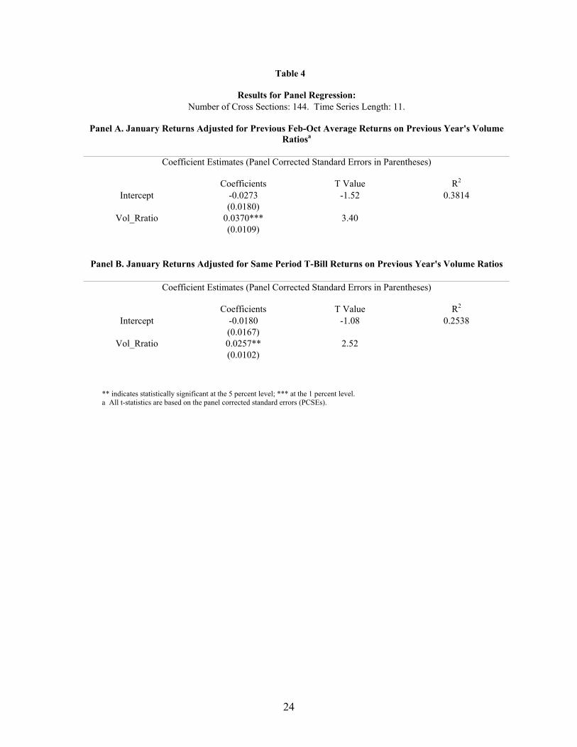
the year-by-year regression results in Table 3.8 The coefficient on ratiovol _ is positive

and statistically significant at the 5 percent level for ten out of the eleven years. In Table

9

4 Panel A, we report the results for the panel regression: the coefficient on ratiovol _ is

positive and significant at the 1 percent level.9 The regression results show that abnormal

returns in January are positively related to the previous year-end trading volume. The R-

squared is 0.3814, indicating that a large proportion of the abnormal returns in January

can be explained by the previous year-end trading activities. As a robustness test, in a

similar set of regressions, instead of controlling for the previous February to October

returns, we subtract from the January fund return the t-bill return for the same month.

The estimates for the panel regressions are reported in Panel B of Table 4. The results are

similar to those in Panel A. In summary, these results suggest that the abnormally high

returns in January can be largely explained by the abnormally high volumes at year-end.

This is consistent with the tax-loss selling hypothesis that the abnormal returns in January

are due to the previous year-end selling pressure on these securities.

In order to examine further whether the observed January return seasonal is

caused by loss-taking trading of individual investors at the previous year-end, we study

the year-end volume and tax-loss selling attributes of municipal bond closed-end funds.

If the January effect is caused by tax-loss selling, we would expect year-end volume to be

greater for funds that declined in price during the year. Since municipal bond closed-end

funds are held mostly by tax sensitive individuals, we expect to observe a relatively clear

relation between year-end trading activities and tax-loss selling attributes. Specifically,

we expect funds to display significant increases in year-end trading volume, i.e. tax-loss

selling at year-end, when they have experienced negative returns.

8 All year-by-year regressions report t-statistics based on the Newey-West (1987) heteroskedasticity and autocorrelation consistent standard errors. 9 All panel regressions report t-statistics based on the panel corrected standard errors (PCSEs).

10

Figure 2 exhibits the average annual return across funds for each year from 1990-

2000. The return for a year is calculated by compounding the monthly average returns.

In 3 of the 11 years, the average annual return is negative: around -3%, -20%, -22% in

1990, 1994 and 1999 respectively. Figure 3 shows the average turnover across funds for

the sample of municipal bond closed-end funds for each month in the 1990-2000 period.

Monthly average turnover is calculated by summing up the turnovers of all available

funds in that month and dividing by the number of funds. (Due to the fact that closed-end

funds have a relatively stable number of shares outstanding, there are no upward or

downward trends in the data.) We find that, in each of the three years with negative

returns, the year-end turnover is indeed larger. The pattern is most prominent in 1994

and 1999, when these funds experience the largest losses. Further, in years following

large loss years, in particular 1995, 1996 and 2000, the year-end turnover is still higher

most likely due to a lag effect. The losses in 1994 and 1999 are so large that the funds

still do not regain their previous prices in the subsequent years of 1995 and 2000. Thus,

investors can continue to realize accrued capital losses at the following year-ends. In

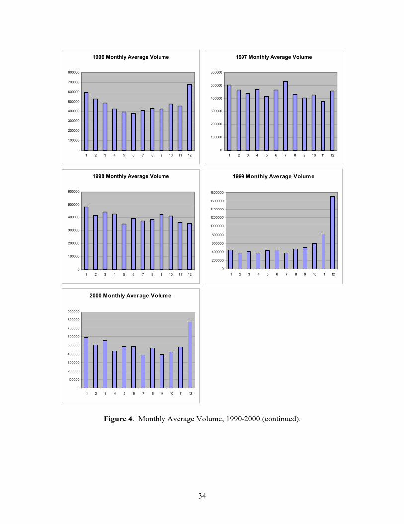
order to see the year-by-year pattern more clearly, we display the monthly average

volume for each year from 1990-2000 in Figure 4. Again, the pattern displayed is not

subject to changes in shares outstanding. Notice that not all years display the same year-

end volume pattern: only in the years of losses and the years subsequent to the large

drops in prices is the year-end volume significantly larger than the volume in the other

months; there is no clear pattern in the other years. In summary, the return and volume

patterns seem to suggest that these fund investors display tax-loss selling behavior at the

end of the year.

11

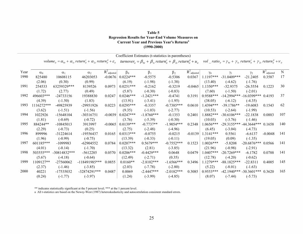
We also run cross-sectional regressions of the year-end volume measures on the

current and the previous year returns for each year from 1990-2000. We again focus on

year-end volume as the average trading volume of November and December. We use

three different measures of year-end volume for each fund:

=itvolume tyearinifundofvolumetradingDecemberandNovemberaverage

tyearinifundofvolumetradingOctobertoFebruaryaverage

tyearinifundofvolumetradingDecemberandNovemberaverageratiovol it =_

The first measure is the average trading volume of November and December, denoted by

volume. The second measure is turnover, defined as the average trading volume of

November and December divided by the number of shares outstanding. This measure is

not subject to variation in the numbers of outstanding shares across funds. Vol_ratio, the

third measure of year-end volume, is defined as the average trading volume of November

and December divided by the average volume from February to October of that the same

calendar year. It measures the year-end volume relative to that of the other months in the

same year for a fund. The relative volume measure controls for the fund-specific and

time-specific fluctuations. For example, noise due to trends in the trading volume of

individual funds is moderated by adjusting the year-end volume by the nine-month

average. Also, the vol_ratio and turnover measures of trading volume allow comparisons

across firms even when their normal trading volumes differ in magnitude.

The current year return of a fund is defined as the monthly return of holding that

fund from January to October in that year. The previous year return is defined as the

tyearinifundofg outstandinsharesofNumbertyearinifundofvolumetradingDecemberandNovemberaverageturnoverit =

12

monthly holding period return of the fund in the previous calendar year, from January to

December. We run the following sets of regressions for each year 1990-2000:

itpitt

citttit returnreturnvolume εααα +++= 210

itpitt

citttit ureturnreturnturnover +++= 210 βββ

itpitt

citttit returnreturnratiovol νγγγ +++= 210_

where creturn and preturn represent the current year return and the previous year return,

respectively.

The coefficient estimates and their corresponding t statistics are reported in Table

5. Among the three year-end volume measures, the relative measures (turnover and

vol_ratio) capture the volume-return relation better than the absolute measure (volume)

as expected. Using turnover as the dependent variable, we find a negative coefficient on

the current year return in all years but 1997. In seven out of the 11 years studied, the

coefficient is statistically significant at the 5 percent level. The coefficient on the

previous year return is negative in all years but 1998, and is significant at the 1 percent

level in 5 years. Using Vol_ratio as the dependent variable, we find that the estimated

coefficient on the current year return is negative and significant at the 5 percent level in

eight years. The estimated coefficient on the previous year return is negative in all 11

years and is significant at the 1 percent level in four years. Furthermore, the negative

relation between the year-end volume and the current year return is most prominent in

1994 and 1999, when funds experience the largest losses (the average annual returns are

around –20% and –22%, respectively) and in years immediately following them. The

negative relation between the year-end volume and the previous year return is strongest

in 1995 and 2000 because of the lag tax-loss effect. Because of the huge losses in 1994

13

and 1999 for municipal bond closed-end funds, in the years immediately following them

the funds still do not fully recover from their previous losses. As a result, investors

continue to gain tax benefits from late-in-the-year loss-taking activities. The regression

results again suggest a negative relation between year-end volume and current / previous

fund returns and confirm the evidence presented in Figures 2 and 3.

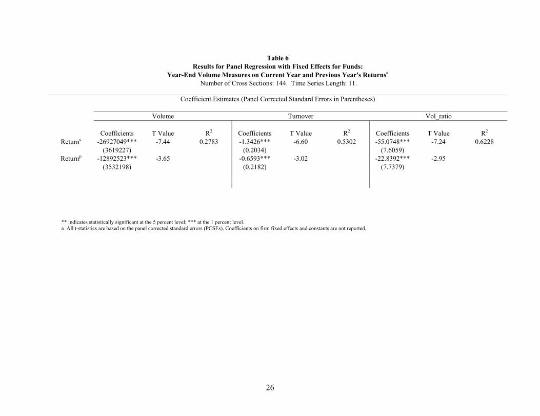
In Table 6, we report the results of the panel regressions with fund fixed effects.

The regressions include a total of 144 closed-end funds in 11 years. 10 The model

specification is very similar to that of Table 5 (the year-end volume measures on the

current and the previous year returns). The fixed effects control for the variations across

funds. The coefficients on the returns are all negative and significant at the 1 percent

level, indicating a negative relation between the year-end volume and past fund returns.

When turnover and vol_ratio are used as volume measures, both R2 values are higher

than 50 percent, indicating that the past fund returns explain a large proportion of the

volume variation. The above findings provide substantial support for the hypothesis that

income tax considerations result in abnormal year-end trading volumes.

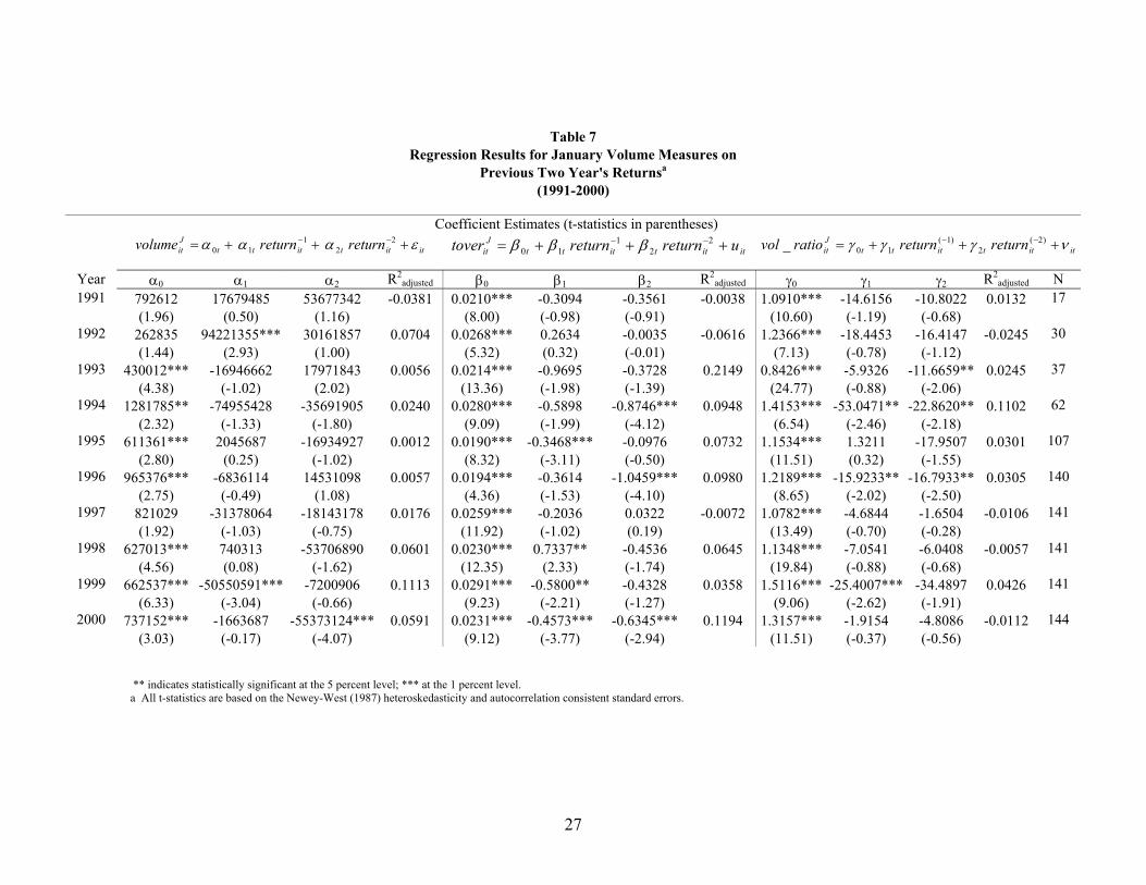
According to the tax-loss-selling hypothesis, the trading volume in January would

also be higher for closed-end funds that have declined in value during the previous years,

since the investors will reinvest in these funds in January. To test this hypothesis, we run

similar regressions as those in Table 5 for each year from 1990 to 2000, using January

volume measures (volume, turnover and vol_ratio) instead of year-end volume measures.

Table 7 summarizes the results. When turnover is used as a proxy for January volume,

the coefficient on the previous year return is negative in eight out of 10 years, and in four

10 We lose some fund observations because we require each fund to have complete return data for the past two years.

14

of those years the coefficient is significant at the five percent level. Further, the

coefficient on the lagged two year return is negative in nine years, in three of those years

the coefficient is statistically significant at the five percent level. When we use vol_ratio

as the dependent variable, the coefficients on the returns are almost all negative, and

three-tenth of them are significant at the five percent level. We notice that the magnitude

of the estimates is generally smaller than that in the November/December regressions.

However, in years with large losses, the negative return-volume relation is still present

and mostly significant. The results of the panel regressions with fund fixed effects are

shown in Table 8. The regressions include a total of 141 closed-end funds in ten years.

All the coefficients on the returns are negative and except for one, all are significant at

the five percent level, indicating a negative relation between the volume in January and

previous fund returns.

In summary, we find evidence that the abnormal returns in January can be

explained largely by the year-end trading activities, which are in turn closely related to

the tax-loss attributes of these funds in the previous two years.

3. Tax-loss selling and brokerage firms

In this section, we examine whether funds associated with brokerage firms display

a stronger pattern of year-end tax-loss selling. The brokerage hypothesis can be viewed

as a direct implication of the tax-loss-selling hypothesis. It posits that closed-end funds

held by investors who receive more tax counseling would experience more tax-loss

selling. Under this hypothesis, funds associated with a brokerage firm are more subject

to tax-loss selling because the brokers would presumably advise the investors to take

advantage of the tax benefits in realizing capital losses at year-end.

15

To test this hypothesis, we include a brokerage dummy and its interaction terms

with the current and previous year returns. We do not estimate the year-by-year

regressions because the number of closed-end funds associated with brokerage firms is

smaller. The fixed-effect panel regression results are shown in Table 9. The three

columns of the table differ in their dependent variables: the first column uses volume as

the year-end volume measure while the second and third columns use turnover and

vol_ratio, respectively. Note that the dummy variable estimates are not listed in the table

because they are picked up by the intercepts (fixed effects). As shown in the table, the

coefficients on the past fund returns and the brokerage-return interaction terms are all

negative and they are significant at the five percent level in all but one case. The

regression results indicate that in addition to the negative return-volume relation,

brokerage counseling is an important factor that explains investor year-end tax-motivated

trading activities. Thus, funds associated with brokerage firms display a stronger pattern

of tax-loss selling at the end of the year, which supports the hypothesis that brokerage

firms advise their clients to engage in tax-motivated trading.

In summary, Table 9 indicates that the end-of-year trading volume of municipal

bond closed-end funds is closely related to the past fund returns. Furthermore, we find

evidence that tax counseling has significant effects on year-end tax-motivated trading as

the brokerage-related closed-end funds display a stronger pattern of tax-loss selling.

IV. Conclusion

The fact that municipal bond closed-end funds are held almost entirely by tax-

sensitive individual investors make them good candidates for the study of tax-loss selling

as an explanation for the January effect. In this paper we find evidence that the tax-loss

16

selling behavior of investors at year-end accounts for a large proportion of the January

effect for this particular set of securities. In particular, we find that the abnormal returns

of the municipal bond closed-end funds in January are positively correlated with the year-

end trading volumes and that the year-end volumes are negatively related to the current

and the previous year returns. Our findings support the tax-loss-selling hypothesis. In

addition, we find that closed-end funds that are associated with brokerage firms display

more tax-loss selling behavior.

In summary, we find a significant January effect among a set of securities that are

held only by individual investors. We provide direct evidence that the observed January

effect can be explained by the tax-loss-selling hypothesis.

17

REFERENCES

Badrinath, S. G., and Wilbur G. Lewellen, 1991, Evidence on tax-motivated securities

trading behavior, Journal of Finance 46, 369-382.

Banz, R. W., 1981, The relationship between return and market value of common stocks,

Journal of Financial Economics 9, 3-18.

Bhabra, Harjeet, Upinder Dhillon, and Gabriel Ramirez, 1999, A November effect?

revisiting the tax-loss-selling hypothesis, Financial Management 28, 5-15.

Blume, M. E., and R. F. Stambaugh, 1983, Bias in computed returns: An application to

the size effect, Journal of Financial Economics 12, 387-404.

Branch, B., 1977, A tax loss trading rule, Journal of Business 50, 198-207.

Brauer, Greggory A., and Eric C. Chang, 1990, Return seasonality in stocks and their

underlying assets: tax-loss selling versus information explanations, Review of

Financial Studies 3, 255-280.

Brickley, J., S. Manaster, and J. Schallheim, 1991, The tax timing option and the discount

on closed-end investment companies, Journal of Business 64, 287-312.

Chan, K. C., 1986, Can tax-loss selling explain the January seasonal in stock returns,

Journal of Finance 41, 1115-1128.

Chang, Eric C., and Michael J. Pinegar, 1986, Return seasonality and tax-loss selling in

the market for long-term government and corporate bonds, Journal of Financial

Economics 17, 391-415.

Constantinides, George, 1984, Optimal stock trading with personal taxes, Journal of

Financial Economics 13, 65-89.

Dyl, Edward, 1977, Capital gains taxation and year-end stock market behavior, Journal

18

of Finance 32, 165-175.

Dyl, Edward, and Edwin Maberly, 1992, Odd-lot transactions around the turn of the year

and the January effect, Journal of Financial and Quantitative Analysis 27, 591-

604.

Eakins, Stan, and Susan Sewell, 1993, Tax-loss selling, institutional investors, and the

January effect: A note, Journal of Financial Research 16, 377-384.

Givoly, Dan and Arie Ovadia, 1983, Year-end induced sales and stock market

seasonality, Journal of Finance 38, 171-185.

Grinblatt, Mark, and Matti Keloharju, 2001, What makes investors trade, Journal of

Finance 56, 589-616.

Haugen, Robert, and Josef Lakonishok, 1988, The incredible January effect: The stock

market’s unsolved mystery (Dow Jones-Irwin, Homewood, Illinois).

Jones, Charles, Douglas Pearce, and Jack Wilson, 1987, Can tax-loss selling explain the

January effect? A note, Journal of Finance 42, 453-461.

Keim, Donald, 1983, Size-related anomalies and stock return seasonality: Further

empirical evidence, Journal of Financial Economics 12, 12-32.

Laing, J. R., 1987, Burnt offerings: Closed-end funds bring no blessings to shareholders,

Barron’s August 10, 1987, 32-36.

Lakonishok, Josef, and Seymour Smidt, 1986, Volume for winners and losers: taxation

and other motives for stock trading, Journal of Finance 41, 951-974.

Musto, David K., 1997, Portfolio disclosures and year-end price shifts, Journal of

Finance 52, 1563-1588.

Odean, Terrance, 1998, Are investors reluctant to realize their losses, Journal of Finance

19

53, 1775-1798.

Peavy, John III W., 1995, New evidence on the turn-of-the-year effect from closed-end

fund IPOs, Journal of Financial Services Research 9, 49-64.

Poterba, James M. and Scott J. Weisbenner, 2001, Capital gains tax rules, tax-loss

trading, and turn-of-the-year returns, Journal of Finance 56, 353-368.

Quinn, J. B., 1987, Playing the closed-end funds, Newsweek August 17, 1987, 65.

Reinganum, Marc, 1983, The anomalous stock market behavior of small firms in January,

Journal of Financial Economics 12, 89-104.

Ritter, Jay, 1988, The buying and selling behavior of individual investors at the turn of

the year, Journal of Finance 43, 701-717.

Ritter, Jay, and Navin Chopra, 1989, Portfolio rebalancing and the turn of the year effect,

Journal of Finance 44, 149-166.

Roll, Richard, 1983, Vas ist das? The turn-of-the-year effect and the return premia of

small firms, Journal of Portfolio Management 9, 18-28.

Rozeff, Michael and William Kinney, 1976, Capital market seasonality: The case of

stock returns, Journal of Financial Economics 3, 379-402.

Seyhun, H. Nejat, 1988, The January effect and aggregate insider trading, Journal of

Finance 43, 129-141.

Sias, Richard W., and Laura T. Starks, 1997, Institutions and individuals at the turn-of-

the-year, Journal of Finance 52, 1543-1562.

Siconolfi, M., 1987, Launching of closed-end funds may ease, Wall Street Journal

November 27, 1987, 29.

Slemrod, Joel, 1982, The effect of capital gains taxation on year-end stock market

20

behavior, National Tax Journal 35, 69-77.

Tinic, Seha M., and Richard R. West, 1984, Risk and return: January vs. the rest of the

year, Journal of Financial Economics 13, 561-574.

21

Table 1 Descriptive Statistics of Municipal Bond Closed-End Funds

Over the Period 1990-2000

a All variables are on a monthly basis. Shares outstanding are in units of one thousand shares.

Year Variable Mean Std Dev Minimum Maximum N SHROUT 27018.94 28225.53 3113 159110

VOL 637467.8 610549.5 21500 4066100

1990 RETX -0.00234 0.028391 -0.10811 0.090909

17

SHROUT 25828.05 25783.04 3119 161132

VOL 653597 555367.4 12300 3702800

1991 RETX 0.004562 0.020862 -0.08955 0.075758

30

SHROUT 21954.01 22673.08 2607 162145

VOL 572512.9 580170.5 5000 5329000

1992 RETX 0.000124 0.027073 -0.10084 0.088496

37

SHROUT 17157.68 19615.5 1007 164230

VOL 477409.9 551556.5 3500 5723700

1993 RETX 0.00159 0.027923 -0.125 0.103896

62

SHROUT 16641.69 19241.33 1007 166371

VOL 557166.8 762609 9200 9102200

1994 RETX -0.01822 0.040001 -0.14851 0.105263

107

SHROUT 17435.09 19180.86 1007 166371

VOL 491234.1 561003.2 8000 6709800

1995 RETX 0.012917 0.034963 -0.08491 0.192771

140

SHROUT 18002.86 21027.94 1007 194960

VOL 473169.8 598960.7 5900 10940500

1996 RETX 0.003026 0.025149 -0.08929 0.130952

141

SHROUT 18106.74 21131.1 1007 194960

VOL 450436.8 618346.5 8800 8608000

1997 RETX 0.00757 0.021618 -0.07767 0.085

141

SHROUT 18039.57 20996.81 1007 194960

VOL 403139.2 513977.3 4800 6470200

1998 RETX 0.003163 0.023215 -0.09884 0.072034

141

SHROUT 17949.15 20039.73 1007 194960

VOL 579137.8 871530.1 1200 15146498

1999 RETX -0.02072 0.02801 -0.19745 0.075438

145

SHROUT 18029.93 20124.97 1007 194960

VOL 497481.7 608110.4 3500 7449100

2000 RETX 0.008166 0.030918 -0.17949 0.139535

165

22

Monthly Return = -0.00192 (Intercept) + 0.02404 (Jan) 11 (-1.03) (2.74)*** Monthly Return = -0.00369 (Intercept) + 0.02007 (Jan) + 0.46942 (Muni index return) 12 (-1.74) (2.31)** (2.80)***

11 Dummies for the other months are also included in the regression, but the estimated coefficients are not statistically different from zero. ** indicates statistically significant at the 5 percent level; *** at the 1 percent level. All t-statistics are based on the Newey-West (1987) heteroskedasticity and autocorrelation consistent standard errors (t-statistics in parentheses). 12 Monthly returns on muni index are available from January 1990 through April 1999.

Table 2

Monthly Average Return for Municipal Bond Closed-End Funds

(1990-2000)

Month Average Return

1 0.0221 2 0.0011 3 -0.0153 4 -0.0025 5 -0.0012 6 0.0065 7 0.0102 8 -0.0033 9 -0.0093

10 -0.0105 11 0.0023 12 0.0009

23

Table 3

Regression Results for January Returns Adjusted for Previous Feb-Oct Average Returns on Previous Year's Volume Ratiosa

(1990-2000)

Coefficient Estimates (t-statistics in parentheses)

ititttitit ratiovolretrretJan εαα ++=− −− 110210

1 _

Year α0 α1 R2

adjusted N 1990 -0.0455** 0.0582*** 0.2029 17

(-2.72) (3.49) 1991 -0.0187 0.0341 0.0834 30

(-0.77) (1.90) 1992 -0.0314*** 0.0429*** 0.2355 37

(-2.78) (4.08) 1993 -0.0079 0.0376** 0.0658 62

(-0.60) (2.47) 1994 0.0008 0.0133** 0.0434 107

(0.11) (2.14) 1995 0.0418** 0.0313*** 0.2142 140

(2.61) (4.79) 1996 -0.0127 0.0307*** 0.2043 141

(-1.65) (6.13) 1997 -0.0133** 0.0203*** 0.0682 141

(-1.99) (3.80) 1998 0.0006 0.0150*** 0.0421 141

(0.11) (2.76) 1999 -0.0539*** 0.0208*** 0.0472 145

(-8.02) (2.86) 2000 0.0245*** 0.0081*** 0.0501 165

(3.14) (2.96)

** indicates statistically significant at the 5 percent level; *** at the 1 percent level. a All t-statistics are based on the Newey-West (1987) heteroskedasticity and autocorrelation consistent standard errors.

24

Table 4

Results for Panel Regression: Number of Cross Sections: 144. Time Series Length: 11.

Panel A. January Returns Adjusted for Previous Feb-Oct Average Returns on Previous Year's Volume

Ratiosa

Coefficient Estimates (Panel Corrected Standard Errors in Parentheses)

Coefficients T Value R2 Intercept -0.0273 -1.52 0.3814

(0.0180) Vol_Rratio 0.0370*** 3.40

(0.0109)

Panel B. January Returns Adjusted for Same Period T-Bill Returns on Previous Year's Volume Ratios


Coefficients T Value R2

Intercept -0.0180 -1.08 0.2538 (0.0167)

Vol_Rratio 0.0257** 2.52 (0.0102)

** indicates statistically significant at the 5 percent level; *** at the 1 percent level. a All t-statistics are based on the panel corrected standard errors (PCSEs).

25

Table 5 Regression Results for Year-End Volume Measures on

Current Year and Previous Year's Returnsa (1990-2000)


itpitt

citttit returnreturnvolume εααα +++= 210 it

pitt

citttit ureturnreturnturnover +++= 210 βββ it

pitt

citttit returnreturnratiovol νγγγ +++= 210_

Year α0 α1 α2 R2

adjusted β0 β1 β2 R2adjusted γ0 γ1 γ2 R2

adjusted N 1990 825480 10608115 46203053 -0.0676 0.0224*** -0.5575 -0.5306 0.0367 1.1197*** -31.0409*** -21.2405 0.3587 17

(2.06) (0.30) (0.99) (6.19) (-1.98) (-1.38) (13.40) (-4.62) (-1.76) 1991 254533 63259329*** 8139526 0.0973 0.0251*** -0.2162 -0.3219 -0.0465 1.1350*** -32.9375 -26.5554 0.1223 30

(1.72) (2.77) (0.49) (5.87) (-0.30) (-0.83) (7.60) (-1.50) (-2.01) 1992 496603*** -24733156 19388830 0.0247 0.0246*** -1.2421*** -0.4741 0.3191 0.9588*** -14.2994*** -16.0399*** 0.4193 37

(4.39) (-1.50) (1.83) (13.91) (-3.41) (-1.95) (38.05) (-6.12) (-4.35) 1993 1116272*** -49825939 -29951926 0.0223 0.0295*** -0.3357 -0.7385*** 0.0610 1.4394*** -39.1786** -19.6083 0.1543 62

(3.62) (-1.51) (-1.56) (9.35) (-1.03) (-2.77) (10.53) (-2.64) (-1.99) 1994 1022926 -15648104 -30316751 -0.0039 0.0247*** -1.8760*** -0.1353 0.2401 1.8882*** -30.6106*** -22.1838 0.0883 107

(1.81) (-0.69) (-0.72) (3.76) (-5.39) (-0.30) (10.03) (-3.76) (-1.46) 1995 884244** -10845013 3913997 -0.0065 0.0139*** -0.7737** -1.9054*** 0.2348 1.0656*** -29.3155*** -44.3644*** 0.1658 140

(2.29) (-0.73) (0.25) (2.75) (-2.48) (-4.96) (6.45) (-3.04) (-4.73) 1996 899996 -31224614 -19556437 0.0165 0.0313*** -0.0755 -0.0215 -0.0139 1.3141*** 0.5561 -6.6137 -0.0048 141

(1.96) (-0.99) (-0.75) (13.39) (-0.33) (-0.11) (19.05) (0.09) (-1.35) 1997 601185*** -1099983 -62904552 0.0784 0.0207*** 0.5679*** -0.7552*** 0.1523 1.0026*** -5.8208 -20.6876*** 0.0566 141

(4.01) (-0.14) (-1.70) (13.32) (2.81) (-3.85) (21.96) (-0.98) (-2.91) 1998 503555*** -30814832*** -5612285 0.0570 0.0206*** -0.4429*** 0.0648 0.0479 1.0407*** -20.7269*** -6.1782 0.0788 141

(5.67) (-4.18) (-0.64) (12.49) (-2.71) (0.35) (12.78) (-4.20) (-0.62) 1999 1109127** -27560062 -118491985*** 0.0855 0.0160** -2.8102*** -1.6566*** 0.3496 1.1279*** -88.1825*** -22.8311 0.4005 145

(2.37) (-1.46) (-3.85) (2.03) (-7.78) (-2.80) (5.22) (-8.01) (-1.63) 2000 40221 -17535032 -32874291*** 0.0487 0.0069 -2.4447*** -2.0182*** 0.3085 0.9553*** -42.1940*** -30.3601*** 0.3620 165

(0.24) (-1.77) (-3.97) (1.24) (-3.99) (-4.85) (8.07) (-7.44) (-5.73)


26

Table 6 Results for Panel Regression with Fixed Effects for Funds:

Year-End Volume Measures on Current Year and Previous Year's Returnsa Number of Cross Sections: 144. Time Series Length: 11.


Volume Turnover Vol_ratio Coefficients T Value R2 Coefficients T Value R2 Coefficients T Value R2

Returnc -26927049*** -7.44 0.2783 -1.3426*** -6.60 0.5302 -55.0748*** -7.24 0.6228 (3619227) (0.2034) (7.6059)

Returnp -12892523*** -3.65 -0.6593*** -3.02 -22.8392*** -2.95 (3532198) (0.2182) (7.7379)

** indicates statistically significant at the 5 percent level; *** at the 1 percent level. a All t-statistics are based on the panel corrected standard errors (PCSEs). Coefficients on firm fixed effects and constants are not reported.

27

Table 7

Regression Results for January Volume Measures on Previous Two Year's Returnsa

(1991-2000)


itittittt

Jit returnreturnvolume εααα +++= −− 2

21

10 itittittt

Jit ureturnreturntover +++= −− 2

21

10 βββ itittitttJit returnreturnratiovol νγγγ +++= −− )2(

2)1(

10_

Year α0 α1 α2 R2adjusted β0 β1 β2 R2

adjusted γ0 γ1 γ2 R2adjusted N

1991 792612 17679485 53677342 -0.0381 0.0210*** -0.3094 -0.3561 -0.0038 1.0910*** -14.6156 -10.8022 0.0132 17 (1.96) (0.50) (1.16) (8.00) (-0.98) (-0.91) (10.60) (-1.19) (-0.68)

1992 262835 94221355*** 30161857 0.0704 0.0268*** 0.2634 -0.0035 -0.0616 1.2366*** -18.4453 -16.4147 -0.0245 30 (1.44) (2.93) (1.00) (5.32) (0.32) (-0.01) (7.13) (-0.78) (-1.12)

1993 430012*** -16946662 17971843 0.0056 0.0214*** -0.9695 -0.3728 0.2149 0.8426*** -5.9326 -11.6659** 0.0245 37 (4.38) (-1.02) (2.02) (13.36) (-1.98) (-1.39) (24.77) (-0.88) (-2.06)

1994 1281785** -74955428 -35691905 0.0240 0.0280*** -0.5898 -0.8746*** 0.0948 1.4153*** -53.0471** -22.8620** 0.1102 62 (2.32) (-1.33) (-1.80) (9.09) (-1.99) (-4.12) (6.54) (-2.46) (-2.18)

1995 611361*** 2045687 -16934927 0.0012 0.0190*** -0.3468*** -0.0976 0.0732 1.1534*** 1.3211 -17.9507 0.0301 107 (2.80) (0.25) (-1.02) (8.32) (-3.11) (-0.50) (11.51) (0.32) (-1.55)

1996 965376*** -6836114 14531098 0.0057 0.0194*** -0.3614 -1.0459*** 0.0980 1.2189*** -15.9233** -16.7933** 0.0305 140 (2.75) (-0.49) (1.08) (4.36) (-1.53) (-4.10) (8.65) (-2.02) (-2.50)

1997 821029 -31378064 -18143178 0.0176 0.0259*** -0.2036 0.0322 -0.0072 1.0782*** -4.6844 -1.6504 -0.0106 141 (1.92) (-1.03) (-0.75) (11.92) (-1.02) (0.19) (13.49) (-0.70) (-0.28)

1998 627013*** 740313 -53706890 0.0601 0.0230*** 0.7337** -0.4536 0.0645 1.1348*** -7.0541 -6.0408 -0.0057 141 (4.56) (0.08) (-1.62) (12.35) (2.33) (-1.74) (19.84) (-0.88) (-0.68)

1999 662537*** -50550591*** -7200906 0.1113 0.0291*** -0.5800** -0.4328 0.0358 1.5116*** -25.4007*** -34.4897 0.0426 141 (6.33) (-3.04) (-0.66) (9.23) (-2.21) (-1.27) (9.06) (-2.62) (-1.91)

2000 737152*** -1663687 -55373124*** 0.0591 0.0231*** -0.4573*** -0.6345*** 0.1194 1.3157*** -1.9154 -4.8086 -0.0112 144 (3.03) (-0.17) (-4.07) (9.12) (-3.77) (-2.94) (11.51) (-0.37) (-0.56)


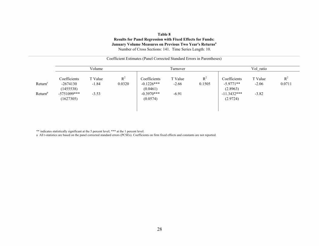
28

Table 8 Results for Panel Regression with Fixed Effects for Funds:

January Volume Measures on Previous Two Year's Returnsa Number of Cross Sections: 141. Time Series Length: 10.



Returnc -2674130 -1.84 0.0320 -0.1226*** -2.66 0.1505 -5.9771** -2.06 0.0711 (1455538) (0.0461) (2.8963)

Returnp -5751099*** -3.53 -0.3970*** -6.91 -11.3432*** -3.82 (1627305) (0.0574) (2.9724)


29

Table 9 Results for Panel Regression with Fixed Effects for Funds: Year-End Volume Measures on

Current Year and Previous Year's Returns with Brokerage Dummy and Interaction Terms Addeda Number of Cross Sections: 144. Time Series Length: 11.



Returnc -24020598*** -7.06 0.2900 -1.1636*** -5.80 0.5665 -51.4226*** -7.53 0.6319 (3402351) (0.2005) (6.8305)

Returnp -11273099*** -3.46 -0.5458** -2.56 -21.7059*** -3.10 (3258121) (0.2134) (6.9959)

Returnc_D -12908240*** -4.76 -0.8001*** -6.27 -15.7831** -2.02 (2711815) (0.1277) (7.8270)

Returnp_D -8378671*** -2.89 -0.5984*** -5.26 -5.9738 -0.70 (2896743) (0.1138) (8.4917)


30

Monthly Average Return for Muni Bond Funds

-2.0%

-1.5%

-1.0%

-0.5%

0.0%

0.5%

1.0%

1.5%

2.0%

2.5%

1 2 3 4 5 6 7 8 9 10 11 12

Figure 1.. Monthly Average Return for Muni Bond Funds, 1990-2000.

31

Average Annual Return

-25.0%

-20.0%

-15.0%

-10.0%

-5.0%

0.0%

5.0%

10.0%

15.0%

20.0%

90 91 92 93 94 95 96 97 98 99 00

Figure 2. Average Annual Return, 1990-2000.

32

Turnover Trend 1990-2000

Dec-90

Dec-00

Dec-99

Dec-96

Dec-95

Dec-94

0

0.01

0.02

0.03

0.04

0.05

0.06

0.07

0.08

0.09

0.1

Jan-9

0Ju

l-90

Jan-9

1Ju

l-91

Jan-9

2Ju

l-92

Jan-9

3Ju

l-93

Jan-9

4Ju

l-94

Jan-9

5Ju

l-95

Jan-9

6Ju

l-96

Jan-9

7Ju

l-97

Jan-9

8Ju

l-98

Jan-9

9Ju

l-99

Jan-0

0Ju

l-00

Figure 3. Monthly Average Turnover Trend, 1990-2000.

33

1990 Monthly Average Volume

0

100000

200000

300000

400000

500000

600000

700000

800000

900000

1 2 3 4 5 6 7 8 9 10 11 12


0

100000

200000

300000

400000

500000

600000

700000

800000

1 2 3 4 5 6 7 8 9 10 11 12


0

100000

200000

300000

400000

500000

600000

700000

800000

1 2 3 4 5 6 7 8 9 10 11 12


0

100000

200000

300000

400000

500000

600000

700000

1 2 3 4 5 6 7 8 9 10 11 12


0

200000

400000

600000

800000

1000000

1200000

1 2 3 4 5 6 7 8 9 10 11 12


0

100000

200000

300000

400000

500000

600000

700000

800000

1 2 3 4 5 6 7 8 9 10 11 12

Figure 4. Monthly Average Volume, 1990-2000.

34


0

100000

200000

300000

400000

500000

600000

700000

800000

1 2 3 4 5 6 7 8 9 10 11 12


0

100000

200000

300000

400000

500000

600000

1 2 3 4 5 6 7 8 9 10 11 12


0

100000

200000

300000

400000

500000

600000

1 2 3 4 5 6 7 8 9 10 11 12


0

200000

400000

600000

800000

1000000

1200000

1400000

1600000

1800000

1 2 3 4 5 6 7 8 9 10 11 12


0

100000

200000

300000

400000

500000

600000

700000

800000

900000

1 2 3 4 5 6 7 8 9 10 11 12

Figure 4. Monthly Average Volume, 1990-2000 (continued).

tax-loss selling and the january effect: evidence … selling and the january effect: evidence from...

Documents