task 3b report: analysis of economic costs and … 3b report analysis of economic costs and benefits...
TRANSCRIPT

Task 3b Report: Analysis of Economic Costs and Benefits of Solar Program
Prepared for the
Massachusetts Department of Energy Resources
By
La Capra Associates, Inc., and Sustainable Energy Advantage, LLC
In association with
Meister Consultants Group and Cadmus
September 30, 2013

Task 3b Report Analysis of Economic Costs and Benefits of Solar Program
About the Massachusetts Department of Energy Resources (DOER) DOER’s mission is to create a cleaner energy future for the Commonwealth, economically and environmentally,
including:
Achieving all cost-effective energy efficiencies,
Maximizing development of cleaner energy resources,
Creating and leading implementation of energy strategies to ensure reliable supplies and improve relative costs,
and
Support clean tech companies and spurring clean energy employment.
DOER is an agency of the Massachusetts Executive Office of Energy and Environmental Affairs (EEA).
About this Report The Team completed our Analysis of Economic Costs and Benefits of Solar Program (Task 3b Report) in support of the
DOER’s Solar Policy Program and post 400-MW policy analysis under a competitive contract awarded to The Cadmus
Group.
As part of the effort, Cadmus, La Capra Associates, Meister Consultants Group, and Sustainable Energy Advantage, LLC,
are to develop five companion reports:
Task 1: Evaluation of Current Solar Costs and Needed Incentive Levels across Sectors Task 2: Comparative Evaluation of Carve-out Policy with Other Policy Alternatives Task 3a: Evaluation of the 400 MW Solar Carve-out Program’s Success in Meeting Objectives Task 3b: Analysis of Economic Costs and Benefits of Solar Program Task 4: Comparative Regional Economic Impacts of Solar Ownership/ Financing Alternatives
Report Authors
La Capra Associates
Alvaro Pereira, PhD (Lead)
Sustainable Energy Advantage, LLC
Robert Grace Mimi Zhang

Task 3b Report Analysis of Economic Costs and Benefits of Solar Program
1
1 Introduction In developing a new policy, it is important to consider and analyze the potential benefits and costs of that policy to
society and the impacted stakeholders. The Massachusetts Department of Energy Resources (DOER) commissioned
Cadmus (Prime Contractor), Sustainable Energy Advantage, LLC (Project Manager), Meister Consultants Group, and La
Capra Associates (collectively known as the Consulting Team) to provide an analysis of Massachusetts solar photovoltaic
(PV) deployment costs and benefits.
1.1 Purpose and Scope
In this report, the Consulting Team provides a detailed economic benefit-cost analysis of a growing solar market in
Massachusetts. Our analysis categorizes, quantifies, and discusses the incremental costs and benefits of the SREC-II Solar
Policy, which consists of a separate modified solar carve-out tier currently under design by DOER to expand the
Commonwealth’s solar PV installations to a target of 1,600 MW by 2020.
The new PV capacity, to be secured under the SREC-II policy, will be 1,600 MW less the final capacity secured under
SREC I. For purposes of this study, the SREC I policy was assumed to enable 400 MW of installed solar PV capacity.1 In
this report, we discuss these various impacts to Massachusetts ratepayers and the economy:
Direct program costs of the SREC-II solar incentives borne by ratepayers
Ratepayer cost savings due to impacts of solar PV penetration on the electricity system clearing price
Cost savings to ratepayers due to delayed or eliminated distribution and transmission utility upgrades
Bill impacts to a typical residential, commercial, and industrial customer
Job creation in Massachusetts and globally
Reductions in imported fuels and greenhouse gas emissions
Potential for increased resilience from solar PV combined with storage during grid outages
The report uses and cites previous information and available literature to supplement the original modeling conducted
specifically for this review of the SREC-II Policy. The work described in this report is related to and builds upon other
tasks commissioned by DOER from the Consulting Team, notably the evaluation of solar costs (Task 1) and policy options
(Task 2).
1.2 Limitations of this Analysis
The analysis in this report represents a high-level calculation of a number of benefit and cost components that could be
used to evaluate the SREC-II policy. The Consulting Team included the most prominent and obvious components, but
there may be a number of benefits (notably regarding impacts on natural gas prices and non-air-emissions-related
environmental impacts2) that were not included or not completely quantified. In addition, realization of benefits
requires use of certain assumptions in terms of solar PV’s interactions with existing market and regulatory mechanisms.
1 DOER has adjusted this target level to accommodate a larger volume but the analysis of this report examines the impacts of an
additional 1200 MW due to SREC-II. 2 For example, solar deployment will undoubtedly displace fossil-fuel generation and thus reduce water usage by these facilities.

Task 3b Report Analysis of Economic Costs and Benefits of Solar Program
2
In this report, we did not attempt to determine the actual cost of the SREC-II Policy; we did use two cost futures to
bound the analysis: one assumed the SREC program cost cleared at the alternative compliance payment (ACP) rate and
another assumed the SREC program cost cleared at the auction floor price. Actual costs (and benefits) of the program
will depend on the specific types (residential, commercial, and utility-scale) of solar deployed and their locations.
Macroeconomic impact modeling of the SREC-II policy was beyond the scope of the current study, but we discuss the
potential job impacts of the SREC-II Policy by drawing upon findings from prior economic analysis of solar expansion in
Massachusetts and elsewhere. The discussion is framed to inform and, we hope, motivate a detailed job impact analysis,
but it should not be considered or used as an estimate of job creation of the SREC-II Solar Policy.
1.3 Organization of this Report
The report is organized as follows:
Section 2 describes the approach used in developing this report.
Section 3 describes some key assumptions used in the report analysis.
Section 4 summarizes the key results of the analysis developed for this report.
Section 5 describes the costs of the SREC-II program.
Section 6 presents the analysis of ratepayer impact, including wholesale market effects, avoided REC payments,
effects, and avoided generation capacity effects. Impacts on typical customer bills are also projected.
Section 7 presents the derivation and results of a statewide benefit-cost analysis, including impacts on emissions
and fuel use.
Section 8 discusses the potential jobs impacts associated with the SREC-II policy.
Section 9 discusses the potential for increased system resilience to result from solar PV combined with energy
storage.
Appendix A describes the key assumptions used in the wholesale market price forecast, with which the Consulting Team
assessed both the cost premium and the wholesale energy market benefits.

Task 3b Report Analysis of Economic Costs and Benefits of Solar Program
3
2 Approach The Consulting Team provides a detailed economic benefit-cost analysis for 1200 MW of solar deployment attributed to
the SREC-II Policy. We conducted both a literature review and an original analysis of a number of benefits to solar
developers and electric consumers as a whole compared to the costs of the SREC-II Policy.
Although a number of studies have quantified the benefits and costs of solar, actual results can vary from location to
location, depending on the local solar policies and investment levels. We use the AURORA production cost model,3
discussed in Appendix A, to accurately capture the particular hourly load shape of the solar deployment and forecast the
revenue streams to solar developers and sponsors and, in turn, calculate the necessary incentive or premium levels for
market penetration of additional solar (as shown in the Task 1 analysis). We supplement the results of this market model
with additional market results from prior studies and literature.
We also examine and calculate how the wholesale energy market impacts would affect all ratepayers. These impacts are
calculated by comparing the proposed policy and build-out case (with expanded solar under SREC-II) to our current
Massachusetts and New England reference case, which includes only current policies (the SREC I Policy and other state
and federal policies).
We make the same comparison in order to analyze the environmental impacts, such as reductions in imported fuels and
changes in air emissions levels, including greenhouse gas emissions.
We will discuss a final set of benefits related to distribution and transmission system reliability and planning derived
from our review of the literature.
We provide estimates and analyze major benefits and costs under a range of cost assumptions and calculate net cost or
benefits and benefit-cost ratios under two different benefit-cost perspectives—a ratepayer perspective and a more
inclusive statewide perspective. Two things are important to note: additional perspectives are possible, and the
objective of this report is to provide estimates for different benefit and cost categories rather than conclude that one
particular perspective is most appropriate.
As shown in Table 1, the Consulting Team analyzed these two perspectives and six categories.
Table 1. Components Considered in Rate Impact and Cost-Benefit Analyses
Solar
Program Costs
Wholesale Energy Market Effects
Avoided
Class I REC
Payments
Generation Investment
Transmission and
Distribution (T&D)
Investment
Carbon and Other Pollutants
Net Electricity Ratepayer Impact
Statewide Benefit-Cost
3 AURORAxmp® is a forecasting and modeling tool developed by EPIS, Inc. (http://epis.com/aurora_xmp/) and is maintained and
adjusted by La Capra Associates for specific policy and project analyses.

Task 3b Report Analysis of Economic Costs and Benefits of Solar Program
4
The order of the categories in the table headings are progressively additive (but not duplicative), such that the statewide
benefit-cost framework in the lower row incorporates the net ratepayer benefit-cost framework in the prior row.
Net electricity ratepayer impact perspective includes categories for the cost of the solar program and various potential
benefit categories, such as:
Wholesale energy market effects as solar facilities displace generation with higher variable and fuel costs in the
energy markets4
Avoidance of Class I REC costs due to the use of a carve-out of Class I renewable portfolio standards RPS
requirements for solar RECs
Avoided investment in generation facilities due to solar deployment
Statewide benefit-cost perspective incorporates potential benefits to Massachusetts residents and businesses that
would not immediately be seen in, or impact, electricity rates and bills.
These two tests differ by the speed and level at which benefits can be captured for ratepayers,5 and the two tests will
converge as these two additional benefit categories are enabled. Two additional benefit categories are included in the
statewide benefit-cost analysis:
Avoided investment in transmission and distribution facilities due to solar deployment
Avoided carbon dioxide (CO2) and other pollutant costs due to the zero air emissions of solar production6
Following discussion of these two benefit calculations, we discuss additional possible impacts, such as potential job
creation or loss. This discussion is necessarily at a high level and relies on other studies, since a job or economic impact
analysis is beyond the scope of the current study.
It is important to note that there are a number of difficult-to-quantify benefits, such as mitigation of generation fuel cost
variability and grid security enhancements, which were beyond the scope of the current study and were not included in
the overall calculations of net benefit. As a result, the benefit-cost estimates shown in this report may understate the
benefit. We describe the interaction between storage and enabling of these difficult-to-quantify benefits (and
supporting capture of additional transmission and distribution [T&D]-related benefits).
4 We calculate only wholesale market effects on energy markets. Solar facilities’ participation in capacity markets has been limited to
participation by utility-owned or sponsored projects (see discussion in Task 1 report). 5 For example, avoidance of transmission and distribution costs would require analysis of the localized benefits of solar and
participation in regulatory proceedings to demonstrate that additional investments would not be needed. By contrast, the benefit categories in the ratepayer analysis have existing mechanisms (for example, wholesale energy and capacity markets and REC markets) to pass along these benefits.
6 The environmental benefits in the benefit-cost analysis of this report consider a limited set of environmental benefits. For example,
solar deployment may serve to reduce water usage by fossil-fueled generation and a number of emissions beyond what are included and quantified here.

Task 3b Report Analysis of Economic Costs and Benefits of Solar Program
5
3 Key Assumptions Key assumptions specific to the SREC-II policy used throughout this report are summarized in this section.
Economic Life of Solar PV Installations. A 25-year economic life is assumed for solar installations.
Time Horizon. The time horizon of the analyses in this report is 2014-2045. This period covers 2014 (the first
year of the expanded solar program) though 2021, the expected year of the last SREC-II installation. Systems
installed in the last year of policy incentives are assumed to produce through 2045.
Nominal Dollars and Discounting. All annual values shown in this chapter are shown in nominal dollars. Net
present value (NPV) calculations use these values with a nominal discount rate of 5.0%.7 Selection of a relevant
discount rate is important, since higher interest rates will, all things equal, reduce the benefit-cost calculations
shown here because toward the beginning of the study period solar cost programs are more heavily weighted
than benefits.
Scale of the SREC-II Policy. Subsequent to the commissioning of this study and through the adoption of
emergency regulations, DOER has committed to set a value higher than the SREC-I policy’s original target of 400
MW; however, the final total MW of SREC-I will not be finalized until mid-2014. Once finalized, the size of the
SREC-II policy will be the difference between the 1600 MW target and the final SREC-I quantity. This analysis
assumes that the SREC-II policy will add 1200 MW to the initial 400 MW target to reach a total goal of 1600 MW.
Federal Investment Tax Credits (ITC) were not assumed to be extended beyond their current statutory
timeframe.
Incremental Policy Analysis. This study considers only the incremental benefits and costs beyond current policy
already in place. The analysis does not include benefits and costs of existing renewable portfolio standards, state
tax credits, and net metering policy.
Alternative Compliance Payment and Auction Floor. Table 2 shows the floor prices and alternative compliance
payment (ACP) used to calculate the low and high cost levels discussed throughout this report.
7 Use of a 5% nominal rate and assumption of 2.5% inflation yields a real discount rate of approximately 2.4%, which is higher
compared to the discount rate used, for example, in the most recent (2013) release of the Avoided Energy Supply Cost (AESC) study used in the cost-effectiveness analyses performed by Massachusetts energy efficiency program administrators. The 2013 AESC study uses a real discount rate of 1.36, which is based on 30-year U.S. Treasury yields as of February 2013, and thus is indicative of an extremely low-rate environment. We elected to use a slightly higher rate consistent with the 2011 AESC study to account for some potential increase in interest rates going forward.

Task 3b Report Analysis of Economic Costs and Benefits of Solar Program
6
Table 2. Auction Floor and ACP Rate
Year Auction Floor
Price ($/MWh) ACP Rate ($/MWh)
2014 285 375
2015 285 375
2016 285 350
2017 271 350
2018 257 350
2019 244 333
2020 232 316
2021 221 300
SREC-II MWh Production. SREC-II production assumed a 13% capacity factor measured at the nameplate. The
total electric system impacts derive from the total quantity of solar production projected from SREC-II
installations. The quantity of SRECs is lower, however, because the assumed policy structure would convey less
than I.0 SREC per MWh produced for the first 10 years of production from each SREC-II facility.
SREC Factors and Distribution of Installations. The SREC factors and distribution of installations across different
categories—see Task 1 and Task 2 reports—impact the expected policy incentive cost and are shown in Table 3.
Table 3. SREC Factors and Distribution of Installation
SREC Factors Distribution of
Installations
Residential (non-Forward Minting) 0.9 9%
Residential (Forward Minting) 0.9 6%
Onsite 0.9 21%
LF-BF 0.8 12%
GRD<500 0.7 12%
Managed 0.6 41%
Forward Minting. Forward minting, whereby solar facilities are provided SRECs prior to generation, was
assumed for a certain percentage of installations (shown in table above).

Task 3b Report Analysis of Economic Costs and Benefits of Solar Program
7
4 Summary of Results Key results from the Consulting Team’s study are these:
Two cost futures bound the analysis with a high-cost future of $1.98 billion and a low-cost future of $1.54 billion
in NPV over the 32-year study period.
The rate impact analysis yields increases between $500 million and $933 million (of NPV) over the entire 32-year
(2014-2045) study period after accounting for wholesale energy market, avoided REC, and avoided generation
capacity cost.
Over the entire study period (on an NPV basis) the solar program is expected to lead to rate impacts between
1.2% and 1.5% of total bills.
Bill impact calculations show that monthly bill increases for a residential customer will average between slightly
less than $1.00 per month to $1.50 per month over the entire study period, depending on which cost futures are
analyzed.
The 1200 MW SREC-II policy is expected to provide approximately 420 MW of reductions during peak load
conditions.
Under a more expansive benefit-cost analysis that included avoidance of transmission and distribution cost and
carbon emissions, solar deployment resulted in a net benefit between $138 million (low-cost future) and $571
million (high-cost future) over the 2014-2045 study period.
Ratios under the statewide benefit-cost test were between 1.07 and 1.37 (corresponding to the high- and low-
cost futures, respectively).
Emissions reductions average 1.4% for CO2, 0.8% for NOx, and 1.7% for SO2 per year.
Solar deployment reduces coal, oil, and natural gas usage from New England generators by 1% to 2% over the
entire study period; 90% of the fuel savings are attributed to natural gas and correspond to approximately a
year’s worth of natural gas usage by Massachusetts’ power generators or 15 months by Massachusetts’
households.
Job impacts were not calculated in this study but, as we found in a review of existing studies, jobs due to
construction, installation, and equipment could lead to job increases ranging between 900 and 6,300 job-years
depending on the underlying economic modeling, consideration of impacts beyond those directly related to
solar spending, and specific solar build-out assumptions. These job impacts would be reduced by depressive
elements, such as increased costs to ratepayers.
If new grid technology enables customers to provide and sell reliability services back to the grid, storage paired
with solar could become an attractive investment and support the avoidance of supply and delivery facilities.

Task 3b Report Analysis of Economic Costs and Benefits of Solar Program
8
5 Costs of the SREC-II Solar Program Costs of the solar program are based on the “premium” or above-market payments to solar owners and developers in
order to construct, service, and operate the facilities. At a high level, this premium is calculated as the difference
between the total costs to build (which incorporates the effect of all federal, state, and other solar incentives, such as
tax credits, grants, low-interest financing, etc.) and the wholesale market revenues received from energy markets and,
for smaller behind-the-meter installations, net metering credits.8
This premium is calculated as a levelized payment over a ten-year period (see the Task 1 report). Solar program costs
start in 2014, the first year of installations under this program, and end in 2030 as the ten-year period ends for
installations within service dates in 2021.
Rather than use the actual premiums required for different types and locations of facilities, we used two cost futures to
bound the cost estimates for this analysis: a high-cost future based on the ACP rate and a low-cost future based on the
auction floor price. Figure 1 shows the build-out that was assumed for the work in this report.
Figure 1. Solar Program Build-Out, 2014-2045.
Application of an assumed 13% capacity factor to these nameplate capacity numbers yields a forecast of solar megawatt
hour (MWh) production that follows a similar curve. We discounted solar generation by the SREC factors to calculate the
number of SRECs generated. For certain customer segments, costs during the initial years of the study period were
expanded due to use of forward minting, which means SRECs are being produced (and transferred to owners) before the
MWh are generated by the solar facilities. Finally, we multiplied SRECs by the premium calculation (shown in Table 2) to
8 Solar facilities are currently eligible for net metering credits. For purposes of this report, we have assumed that the net metering
program will continue and operate independently of the solar program. As a result, we did not include the costs of the net metering payments to solar facilities in the analysis shown below, thereby assuming that such payments could have been made to any eligible facility rather than simply the solar program facilities.
0
200
400
600
800
1000
1200
1400
Cu
mu
lati
ve M
W I
n S
erv
ice

Task 3b Report Analysis of Economic Costs and Benefits of Solar Program
9
generate SREC costs per year, which we used in the benefit-cost calculations shown in Figure 2. In total, solar costs range
from $1.54 billion to $1.98 billion in NPV for the low-cost future (using premium calculations based on the auction floor)
and the high-cost future (using premium calculations based on the ACP), respectively.
Figure 2 shows the data supporting this discussion for the period 2014-2035. As we described, solar generation
continues after this period and declines to zero by the end of 2045 as solar facilities reach the end of their useful lives.
Figure 2. Solar Generation and Market Costs
0
200000
400000
600000
800000
1000000
1200000
1400000
1600000
0
50
100
150
200
250
300
350
2014 2015 2016 2017 2018 2019 2020 2021 2022 2023 2024 2025 2026 2027 2028 2029 2030 2031 2032 2033 2034 2035
Sola
r Ge
ne
rati
on
, MW
h p
er y
ear
SREC
Co
st, m
illi
on
$ p
er
year
Program Year
SREC Market CostsAt ACP Rate
At AuctionFloor Price
Solar Generation, MWh/yr

Task 3b Report Analysis of Economic Costs and Benefits of Solar Program
10
6 Ratepayer Impact This section discusses ratepayer impacts and includes benefits and costs (or avoided costs) that would impact
Massachusetts ratepayers in a direct and quantifiable manner. This net-rate impact concept can be considered an
estimate of the ultimate cost responsibility that all Massachusetts ratepayers will eventually pay.
Rate impacts are calculated by adding various benefit components to the cost levels described above and shown in
Figure 2. The formula for rate impacts is shown here and the following subsections address each of its components:
Ratepayer Impacts = SREC Cost + Wholesale energy market effects
+ Avoided Class I REC Payments + Avoided Generation Capacity Costs9
6.1 Wholesale Market Effects
Wholesale energy market effects are considered a benefit to consumers, that is, to the extent that this impact effects a
transfer from producers to consumers that is not accounted for in other energy products or market mechanisms, and
thus serves to reduce the level of solar program costs. We calculated these energy market effects of deploying solar
compared to a base case (see Appendix A for a list of assumptions) that excludes the 1200 MW assumed SREC-II build-
out shown in Figure 1. We provide the calculation of these effects in this section but acknowledge that there may be
different views regarding the persistence of these benefits and their transferability to retail bills paid by ratepayers.
Therefore, we use the assumptions and methodology described in the 2013 Avoided Energy Supply Component Study
(AESC) regarding the calculation of demand-reduction-induced-price-effects (DRIPE).10 At a high level, AESC’s
methodology consists of first calculating a gross DRIPE impact, which for this study we calculated as the difference
between the base case (business-as-usual) wholesale electric energy prices and the prices that reflect the impact of the
solar program build-out.
We then adjusted these price differences per unit ($/MWh) using a dissipation schedule, shown in Table 4 (and based on
Exhibit 7-9 of the 2013 AESC Study). This dissipation schedule considers the declining persistence in energy market
effects as market participants adjust their bidding and other market behavior to account for (and anticipate) the market
impacts of additional solar deployment.
9 Benefit components serve to reduce costs and thus would have an opposite sign to costs. Thus, assuming that SREC cost is positive
in this equation, the three benefit components would have a negative sign and would, in effect, be subtracted from cost. 10
http://www.synapse-energy.com/Downloads/SynapseReport.2013-07.AESC.AESC-2013.13-029-Report.pdf

Task 3b Report Analysis of Economic Costs and Benefits of Solar Program
11
Table 4. Energy Market Effect Adjustments
Production Year(s) Dissipation
% Load Subject to
Solar Market Effects 1 13% 18%
2 18% 72%
3 21% 81%
4 28% 90%
5 34% 90%
6 47% 90%
7 59% 91%
8 70% 91%
9 81% 91%
10 91% 92%
11-end of study period 100% 92%
The next step involves multiplying the adjusted market effects ($/MWh) by the relevant load levels (from the business-
as-usual case) to estimate the total dollar value saved by consumers from solar resources.
For the calculations in this study, we assumed any savings to consumers due to wholesale energy market effects that
apply to Massachusetts load would be subject to changes in spot energy market conditions. While the load-serving
entities that are responsible for most of Massachusetts’ load have divested their generation assets and regularly procure
energy to serve their load through frequent short-term market solicitations, assuming that customer savings applies to
all load may overstate the energy market benefits due to existing terms of long-term contracts. For example, there may
be long-term contracts for load that have been entered into prior to deployment of solar in a particular year or for
production used for self-supply by resources owned or controlled by load-serving entities that are not conducted
through the spot market and thus would not be impacted by solar deployment. Therefore, we apply an adjustment (see
Table 4, based on Exhibit 7-7 of the 2013 AESC) that reduces the potential effects especially during the early years of the
study period.
Figure 3 compares the gross market effects ($/year) to the net market effects calculated after making the dissipation
and load adjustments.11 The data show a peak year around 2038 with a gross market effect of about $65 million; the
gross market effects then decline until the end of the study period as solar facilities retire and less generation
contributes to energy markets. By contrast, net market effects peak in 2021 at about $16 million and then dissipate to
zero in 2030 as the energy market effects dissipate for the last SREC-II installations.
11
Gross market effects show some volatility due to changing market (supply/demand) conditions; this volatility is not a function of the SREC program assumptions.

Task 3b Report Analysis of Economic Costs and Benefits of Solar Program
12
Figure 3. Wholesale Energy Market Effects, Gross vs. Net, 2014-2045
6.2 Avoided Class I REC Payments
In Massachusetts, renewable portfolio standards require non-municipal-utility load serving entities (LSEs) to supply a
certain percentage from renewable (Class I) generation, which is usually the acquisition of RECs or payment of the ACP.
The solar PV program carves out a portion of this requirement, essentially reducing the requirements on LSEs, and thus
can be included as an avoided cost (or benefit) of the program to ratepayers.
Prices for Class I RECs for 2014-2030 were derived from Figure F-1 of the 2013 AESC study and adjusted for inflation for
use in the ratepayer impact calculations; the Consulting Team assumed that prices after 2030 remain constant (in real
terms) at the 2030 level (Figure 4). These prices were multiplied by the SRECs generated (Figure 2) to calculate a stream
of avoided Class I REC costs.
Solar facilities also produce Class I RECs independent of SRECs (after the first 10 years of production), but the potential
revenues from sale of these RECs are already embedded in the cost estimates and thus were not included as a separate
benefit in order to avoid double-counting.
$-
$10,000,000
$20,000,000
$30,000,000
$40,000,000
$50,000,000
$60,000,000
$70,000,000
Gross Net

Task 3b Report Analysis of Economic Costs and Benefits of Solar Program
13
Figure 4. Assumed Class I REC Prices, 2014-2045
6.3 Solar Contribution to Electric System Peaks A number of benefit categories relate to the ability of solar to displace delivery and supply resource investments during
times of peak electric demand. To estimate solar PV’s contribution to meeting peak need, a percentage of nameplate
(less than 100%) needs to be applied. But to provide an accurate estimate, a detailed analysis on the specific solar
facilities’ location and system load shapes would have to be conducted. Not surprisingly, estimates for this factor vary by
location and particular treatment of the solar resource.12
For this report, we relied upon a 2006 NREL study that contained Massachusetts-specific data.13 That study calculated
solar’s effective load-carrying capability (ELCC), which can be defined as the ability of a generator to increase load-
carrying capability of a utility or region without causing loss of load. Calculation of ELCC involves examining the
coincidence between demand and generation; the NREL study used actual utility data (load and solar generation) from
across the United States and extrapolated the sample results to conditions in different states. ELCC values are a function
of the penetration of solar (with greater penetration reducing the ELCC values) and the geometries of the solar facilities
with two-axis tracking as the ideal case and southwest-facing 30o-tilt as the worst case.
Values for Massachusetts ranged from 26% to 56% depending on the penetration level and the geometry. The south-
facing 30o-tilt values are shown in Table 5 for different solar penetration levels.
12
See, for example, J. Rogers, K. Porter “Summary of Time Period-Based and Other Approximation Methods for Determining the Capacity Value of Wind and Solar in the United States.” National Renewable Energy Laboratory, March 2012, and “Methods to Model and Calculate Capacity Contributions of Variable Generation for Resource Adequacy and Planning.” NERC, May 2011.
13 R. Perez, R. Margolis, M. Kmeicik, M. Schwab, and M. Perez, “Update: Effective Load-Carrying Capability of Photovoltaics in the
United States.
$-
$10.00
$20.00
$30.00
$40.00
$50.00
$60.00
$70.00
2014 2016 2018 2020 2022 2024 2026 2028 2030 2032 2034 2036 2038 2040 2042 2044

Task 3b Report Analysis of Economic Costs and Benefits of Solar Program
14
Table 5. ELCC Values for Different Solar Penetration Levels
Penetration 2% 5% 10% 15% 20%
ELCC Values 45% 41% 35% 30% 26%
An examination of peak forecasts for Massachusetts compared to the 1600 MW build-out yields a maximum penetration
of solar in 2020 of 10.9% and averages about 9% over the study period.14 Therefore, we used 35% for ELCC, assuming a
10% penetration, and determined that the 1200 MW nameplate capacity of the solar program would provide
approximately 420 MW of peak contribution on a statewide basis.
6.4 Avoided Generation
We used the Exhibit 5-14 of the 2013 AESC study for avoided capacity cost in order to approximate solar’s displacement
of generation resources by effectively reducing the corresponding peak loads that would be procured (through the net
installed capacity requirement or NICR) in ISO-NE’s forward capacity market.15 The AESC forecast assumed that capacity
prices would eventually rebound from current prices in 2020 and that shortage conditions would drive capacity prices
into the future (through 2030).
We further assumed that these conditions would continue to the end of the study period. Though actual capacity prices
may differ (lower or higher) from these price streams, we have essentially valued the capacity contribution of solar in
later years of the study at the cost of providing marginal capacity similar to price levels necessary to procure peak
generating resources to meet capacity needs.
In the AESC study, this stream of forecasted prices16 is further grossed up for reserves (17.2%), distribution losses (8%),
transmission or pool transmission facilities (PTF) losses (1.5%), and a default wholesale risk premium (9%). For purposes
of this report, we did not use the default wholesale risk premium but did maintain the other assumptions in order to
account for solar’s important characteristic of being located relatively close to load. Figure 5 shows the costs (on a $/kw-
year basis) used in the rate-impact analysis.
14
1600 MW/15,540 MW Peak Forecasted Load. This forecasted load is at the wholesale level, thus penetration at retail levels will be slightly lower.
15 As such, we do not assume that solar facilities would participate directly in the forward capacity auction, rather the impact would
be indirectly felt by reducing the amount that would have to be procured in these auctions. 16
The AESC study did not provide prices on a zonal basis, and it appears that the FCM will incorporate the potential for zonal separation in Massachusetts, but a more detailed FCM forecast was not available.

Task 3b Report Analysis of Economic Costs and Benefits of Solar Program
15
Figure 5. Avoided Generation Capacity Costs
To calculate avoided generation capacity benefits, we applied the avoided capacity prices shown in this figure to the
peak contribution value provided by solar. We excluded avoided capacity through May 2018, since net ICR values have
already been finalized for the upcoming FCM auction for the 2017-2018 power year to be held in February of 2014, as
well as prior auctions.
6.5 Rate Impact Calculation
Figure 6 and Figure 7 show the components used to calculate the net rate impact for each year in the study period under
ACP and auction floor cost conditions, respectively. Benefits are positive and costs are negative. An examination of the
net ratepayer impacts illustrate some offsetting benefits during the payment of SREC-related costs, but only generation
capacity cost avoidance benefits continue beyond 2028, resulting in rate savings as SREC costs disappear in 2030 for the
high cost (ACP) level; rate savings are enabled one year earlier (in 2027) under low cost (auction floor) conditions.
$-
$50.00
$100.00
$150.00
$200.00
$250.00
$300.00
20
14
20
16
20
18
20
20
20
22
20
24
20
26
20
28
20
30
20
32
20
34
20
36
20
38
20
40
20
42
20
44
$/k
w-Y
ear

Task 3b Report Analysis of Economic Costs and Benefits of Solar Program
16
Figure 6. Ratepayer Impact Components, with Cost at ACP, 2014-2045
Figure 7. Ratepayer Impact Components, with Cost at Auction Floor, 2014-2045
$(350)
$(300)
$(250)
$(200)
$(150)
$(100)
$(50)
$-
$50
$100
$150M
illio
n $
Solar Program Costs Wholesale Energy Market Effects Avoided REC Payments Avoided Gen Rate Impact
$(350)
$(300)
$(250)
$(200)
$(150)
$(100)
$(50)
$-
$50
$100
$150
Mill
ion
$
Solar Program Costs Wholesale Energy Market Effects Avoided REC Payments Avoided Gen Rate Impact

Task 3b Report Analysis of Economic Costs and Benefits of Solar Program
17
Table 6 shows the rate components in terms of net present value using the discount rate discussed earlier. The sum of
the components yields a total rate impact of between $500 and $933 million over the entire 32-year (2014-2045) study
period.
Table 6. NPV of Rate Impact Components, Cost at ACP vs. Auction Floor (million $)
Cost at
ACP Cost at
Auction Floor
Solar Program Costs (1,976) (1,543)
Wholesale Energy Market Effects 87 87
Avoided REC Payments 184 184
Avoided Generation Capacity Costs 772 772
Rate Impact (933) (500)
Retail rate impact (as a percentage of bills) is calculated as the total rate impact (as shown in Table 6) divided by total
(forecasted) annual electricity expenditures in Massachusetts. Thus, it is assumed for these purposes that the total costs
of the policy options will be borne by all non-municipal utility ratepayers in proportion to their total bill.17
We used the Energy Information Administration’s (EIA’s) Annual Energy Outlook 2013 forecast for the Northeast region
along with historical Massachusetts revenue data to calculate weighted average total retail revenue (delivery and supply
charges) for each year in the study period.18 For years after 2040 (the last year in the EIA forecast), the 2030-2040
compound average annual growth rate of 2.3% was applied in each year. Figure 8 below shows the forecasts of total
retail electricity expenditures in nominal dollars.
17
Municipal utilities’ customers were assumed to be exempt from solar program costs (and participation) due to their exemption from retail choice and RPS requirements. Hence, total Massachusetts revenues were reduced by 13% to only account for investor-owned distribution customers.
18http://www.eia.gov/forecasts/aeo/

Task 3b Report Analysis of Economic Costs and Benefits of Solar Program
18
Figure 8. Total Retail Electricity Expenditures (Non-Municipal Utility Customers),
Massachusetts, 2014-2045
Rate impacts as a percentage of total bills were calculated by taking the solar rate impact calculation for each year and
dividing by the total retail expenditures for that year. For example, in 2020, rate impacts reach their peak between $170
and $240 million, depending on the cost future. Dividing that figure by the total forecasted retail electricity expenditures
in that year of approximately $7.2 billion yields a rate increase between 2.4% and 3.4% for that year.
The annual rate impact as a percentage of total bills is shown for each year in the study period in Figure 9 for both cost
futures. Bill impacts peak in 2020, in the last full year of the deployment, and decline thereafter as increases in overall
electricity costs outpace the increase in ratepayer impacts from the solar program as projects reach the end of their
useful lives. Over the entire study period (on an NPV basis), the solar program is expected to lead to rate impacts
between 1.2% and 1.5%.
0
2000
4000
6000
8000
10000
12000
14000
20
14
20
15
20
16
20
17
20
18
20
19
20
20
20
21
20
22
20
23
20
24
20
25
20
26
20
27
20
28
20
29
20
30
20
31
20
32
20
33
20
34
20
35
20
36
20
37
20
38
20
39
20
40
20
41
20
42
20
43
20
44
20
45
Mill
ion
No
min
al $

Task 3b Report Analysis of Economic Costs and Benefits of Solar Program
19
Figure 9. Rate Impact as a Percentage of Total Bills, 2014-2045
6.6 Bill Impacts
A final way to examine rate impacts is to apply the above annual percentage impacts to monthly or annual bills. Table 7
shows some summary metrics for rate impacts on three representative customer groups.
Table 7. Monthly Rate Impacts by Customer Type, ACP vs. Auction Floor
Average Monthly Usage
(Kwh)
ACP Auction Floor
Average Rate Impact
Max Rate Impact
Average Rate Impact
Max Rate Impact
Residential 746 $1.48 $3.49 $0.91 $2.44
Commercial 4,475 $8.65 $20.43 $5.36 $14.31
Industrial 79,297 $142.94 $337.80 $88.62 $236.53
The calculations show that monthly bill impacts for a residential customer will average between slightly less than $1.00
per month to $1.50 per month over the entire study period. It is important to note that the estimates shown above are
illustrative, since actual costs will depend on specific rates filed by the relevant local distribution companies.
-1.50%
-1.00%
-0.50%
0.00%
0.50%
1.00%
1.50%
2.00%
2.50%
3.00%
3.50%
4.00%
20
14
20
15
20
16
20
17
20
18
20
19
20
20
20
21
20
22
20
23
20
24
20
25
20
26
20
27
20
28
20
29
20
30
20
31
20
32
20
33
20
34
20
35
20
36
20
37
20
38
20
39
20
40
20
41
20
42
20
43
20
44
20
45
% o
f To
tal B
ill
ACP Auction Floor

Task 3b Report Analysis of Economic Costs and Benefits of Solar Program
20
7 Statewide Benefit-Cost Analysis For the benefit-cost calculations, we use the calculations from the ratepayer impact analysis above and consider two
additional benefit (or avoided cost) categories related to electricity delivery and emissions. Specifically,
Statewide Cost-Benefit = SREC Cost + Wholesale energy market effects + Avoided REC Payments + Avoided
Generation Capacity Costs + Avoided Transmission and Distribution Investment +
Avoided Carbon (and Other Emissions) Effects19
The additional T&D benefit category relates to the ability of solar to displace delivery-related investments during peak
times. As in the case of the avoided generation cost, a percentage of nameplate (less than 100%) needs to be applied to
estimate solar’s contribution to meeting peak needs.
The following subsections address the two additional components of this formula.
7.1 Avoided T&D Avoided generation costs were included as a component of the rate impact in the prior section. Solar can also avoid the
construction of transmission and distribution facilities that connect these generation resources to load centers. We
acknowledge that there may be synergies between additional T&D (but less with distribution) and generation
resources,20 but there is currently enough separation in the two planning and market processes underlying delivery and
supply infrastructure that we have, for this benefit-cost test, assumed that avoided T&D benefits would be additive to
the avoided generation capacity benefits calculated for rate impact purposes.
In terms of valuing the avoided T&D, we used data from Exhibit G-1 of the 2013 AESC study, which is based on a survey
of New England utilities; data for Massachusetts utilities are replicated in Table 8.
Table 8. Massachusetts Utilities’ Transmission and Distribution
Year $
Transmission $/kW-Year
Distribution $/kW-Year
National Grid MA 2013 88.64 111.37
NSTAR 2011 21.00 68.69
Unitil MA 2013 NA 171.15
WMECO 2011 22.27 76.08
19
For this equation, costs are considered as a negative term, thus benefits are positive and added to the cost estimate. 20
Generation resources can, in certain cases, provide reliability benefits as an alternative to transmission investment, thus it is possible for the two types of facilities to be substitutes rather than complements. The same is also true of distribution facilities, but non-transmission alternatives (NTA) analysis has been more readily conducted in New England than non-distribution system alternatives.

Task 3b Report Analysis of Economic Costs and Benefits of Solar Program
21
These values were converted to nominal dollars and weighted by each utility’s contribution to peak load for use in the
benefit-cost calculations. The calculated values are shown in Figure 10. Prices were assumed to be constant in real terms
and only increase for inflation (as reflected in the GDP-PI).21
Figure 10. Avoided Transmission and Distribution Costs, Massachusetts, 2014-2045
7.2 Avoided Emissions Effects The final component in the benefit-cost formulation involves reduction in emissions costs due to fossil fuel emissions
displaced by solar production. In similar fashion to the calculation of gross wholesale energy market effects, we
compared the output of the AURORA-based Northeast Market Model ( NMM) with the SREC-II deployment to a base
case without this incremental solar capacity. Changes to three emissions—CO2, sulfur dioxide (SO2), and nitrogen oxides
(NOx)—were examined and monetized using allowance price prices from the 2013 AESC (see Exhibit 4-1 from that
study).
Overall, there was little impact on SO2 and NOx emissions of displacement of generation resources by solar, with
maximum annual percentage reductions in New England and New York emissions of 4.4% and 1.4%, respectively. This
low level of impacts is mostly due to movement away from oil- and, more recently, coal-powered generation to newer,
natural gas-powered generation, which produces these emissions at much lower levels. In addition, NOx and SO2
allowance prices are forecasted to stay low.22 As a result, we have combined the NOx and SO2 monetized avoided
emissions impacts with the CO2 emissions impacts.
For CO2 emission-allowance monetization, we used the pricing based on lower Regional Greenhouse Gas Initiative
(RGGI) caps (91 million compared to 165 million tons) announced in February 2012. Analysis subsequent to this
21
This assumption is conservative compared to the recent annual increases in transmission costs and rates in New England. 22
For example, see Exhibit 4-1 of the 2013 AESC report.
$-
$50.00
$100.00
$150.00
$200.00
$250.00
$300.00
20
14
20
16
20
18
20
20
20
22
20
24
20
26
20
28
20
30
20
32
20
34
20
36
20
38
20
40
20
42
20
44
$/k
w-Y
ear
Avoided Transmission Avoided Distribution

Task 3b Report Analysis of Economic Costs and Benefits of Solar Program
22
announcement indicated that prices would rise from about $4 per short ton (2010$) to over $10 in 2020. Prices were
further assumed to remain at 2020 levels (in 2010$) throughout the remainder of the study period.
Figure 11 shows the assumed prices (in nominal dollars) and the emissions impacts of the solar programs for each year
of the study period. 23 The figure shows the assumption of inflation growth for emission prices following 2020 and the
declining emissions impacts as solar facilities begin to retire.
Figure 11. CO2 Allowance Prices and Emissions Impacts of Solar Program
We also calculated fuel impacts of the solar deployment (Table 9). Solar facilities reduce fossil fuel usage by generators
due to displacement. This benefit was not explicitly included in the benefit-cost analysis, because some of this benefit
category is transferred via the emissions valuation and energy market impacts already included; thus, we did not want
to double-count benefits. The table below shows the fuel usage impacts that resulted from our production cost
modeling.
Table 9. Fuel Usage Impacts of SREC-II Policy
Total (MMBtu) % of Total
Usage
Coal (15,380,921) -2%
Oil (112,244) -1%
Natural Gas (163,717,334) -2%
23
Emissions Impacts are shown for New England and New York to approximate the RGGI region; there may be additional emissions in other RGGI states, but this impact will be small due to distance and import/export constraints. Emissions impacts in any particular year are a function of a number of variables including actual dispatch, imports/exports between regions, unit availability, fuel prices, and load levels. Thus, annual emissions impacts may be volatile on a year-to-year basis.
-
0.10
0.20
0.30
0.40
0.50
0.60
0.70
0.80
0.90
1.00
0
5
10
15
20
25
20
14
20
15
20
16
20
17
20
18
20
19
20
20
20
21
20
22
20
23
20
24
20
25
20
26
20
27
20
28
20
29
20
30
20
31
20
32
20
33
20
34
20
35
20
36
20
37
20
38
20
39
20
40
20
41
20
42
20
43
20
44
20
45
Mill
ion
s o
f Sh
ort
To
ns
$/S
ho
rt T
on
CO2 Emissions CO2 Price

Task 3b Report Analysis of Economic Costs and Benefits of Solar Program
23
Not surprisingly, reductions were greatest for natural gas,24 due to that fuel’s increasing usage in electric generation
with the opposite conclusion for oil-powered generation. The natural gas savings shown above correspond to
approximately a year’s worth of natural gas usage by Massachusetts’ power generators or 15 months of Massachusetts’
household usage.
7.3 Benefit-Cost Calculations Figure 12 and Figure 13 show the components used to calculate the benefits and costs for each year in the study period
under ACP and auction floor cost conditions, respectively. A comparison of these figures to Figure 6 and Figure 7 (the
analogous figures for rate impact) show the additional large contributions played by avoided T&D. This benefit category
serves to offset some of the solar program costs during most of the years in the 2014-2030 period. These benefits are
expected to continue throughout the study period with decreases tracking the end of the useful lives for the solar
facilities.
Figure 12. Benefit-Cost Components, ACP, 2014-2045 (nominal $)
24
Solar facilities will reduce the demand for natural gas (and other fossil fuels) thus some price impact should be expected. We did not attempt to measure the impact of such price impacts and did not include this benefit in the cost-benefit or rate impact calculations.
$(400)
$(300)
$(200)
$(100)
$-
$100
$200
$300
Mill
ion
$
Solar Program Costs Wholesale Energy Market Effects Avoided Emissions
Avoided REC Payments Avoided T&D Avoided Gen
All Benefit-Cost Components

Task 3b Report Analysis of Economic Costs and Benefits of Solar Program
24
Figure 13. Cost-Benefit Components, Auction Floor, 2014-2045
Table 10 shows the rate components of the benefit-cost components in terms of net present value using the discount
rate discussed earlier; the program costs and first three benefit components are identical to those used in the ratepayer
impact calculation. The sum of the components yields a net benefit of between $138 and $571 million over the 2014-
2045 study period.
Table 10. NPV of Cost-Benefit Components, ACP vs. Auction Floor ($ Millions)
ACP Auction Floor
Solar Program Costs (1,976) (1,543)
Wholesale Market Effects $87 $87
Avoided REC Payments $184 $184
Avoided Generation Capacity Costs $772 $772
Avoided Emissions $122 $122
Avoided T&D $949 $949
Net Benefit 138 571
Benefit-cost Ratio 1.07 1.37
The final row of the table shows that the solar program has benefit-cost ratios greater than one, largely due to the
avoidance of T&D and generation.
$(400)
$(300)
$(200)
$(100)
$-
$100
$200
$300
Mill
ion
$
Solar Program Costs Wholesale Energy Market Effects Avoided Emissions
Avoided REC Payments Avoided T&D Avoided Gen
All Benefit-Cost Components

Task 3b Report Analysis of Economic Costs and Benefits of Solar Program
25
8 Potential Job Impacts As discussed throughout the sections above, the above analysis did not consider a number of environmental benefits,
nor did it consider macroeconomic and job impacts due to increased spending related to deployment of the solar
program. That is, the solar program costs used above in the benefit-cost analysis are revenues to solar owners and
developers who utilize these revenues to purchase equipment and hire labor to construct, operate, and maintain the
solar facilities. Thus, the portion of this additional economic activity that would occur within the state could be counted
as a separate benefit. Similarly, in order to conduct a balanced benefit-cost analysis, we would also have to include the
economic activity that would otherwise occur (notably, related to avoided generation and T&D costs) but is now avoided
due to the development of solar. Finally, any net rate impacts would also have to be included in a full jobs or economic
impact analysis.
Such an analysis is beyond the scope of the current task, but in this section we provide some discussion of the possible
job impacts of the solar deployment to Massachusetts. This discussion is based on a brief literature review and publicly
available models, such as the JEDI economic impact model.25 Additional discussion of job impacts can be found in the
Task 4 report.
The most relevant study to the current task is an economic impact analysis that was conducted by REMI for the SREC-I
Policy,26 which was supposed to reach its 400 MW target by 2018. That study provided economic impact analysis due to
construction and energy cost savings, but the meaning of the latter category is unclear given the rate increases
calculated above. As a result, we concentrated on the construction related impacts, which were calculated for the 305
MW assumed to be built between 2012 and 2018; 95 MW had already been installed by the end of 2011.
In total, the results showed that 2,214 job-years were to be generated due to construction or installation (including
inputs) during the 2012-2018 period. Dividing this figure by the 305 MW yields approximately 7.3 jobs per MW.
Application of this ratio to the 1200 MW build-out results in 8711 jobs over the 2014-2021 installation/construction
period or supporting about 1,089 jobs per year.27 These jobs results would be for Massachusetts and use the REMI
model with embedded assumptions of 0.63, 0.56, and 0.58, as the portion of total demand for installation that would be
supplied in Massachusetts for residential, commercial, and utility-scale installations, respectively; hence, job increases in
total (including outside of the state) would average about 1,845 per year over this period based on the study results.
The work described in the Task 4 report of this consulting work for DOER utilized the JEDI model and calculated
economic impacts per 1,000 residential installations. Assuming 5 kW per installation yields impacts for 5,000 kW or 5
MW. Total job impacts from the construction and installation expenses totaled 136 and 211 jobs for the third-party and
direct ownership constructs, respectively. Conversion to jobs per MW yields 27.2 and 42.2, which are much higher than
the ratios calculated based on the REMI analysis described previously. Of course, the REMI results were based on a
25
JEDI stands for “Jobs and Economic Development Impact” and was developed by the National Renewable Energy Laboratory, More information on JEDI is available at www.nrel.gov/analysis/jedi/about_jedi.html.
26 “Modeling the Economic Impacts of Solar PV Development in Massachusetts.” Presentation to the New England Energy and
Commerce Association Renewables and Distributed Generation Committee, March 28, 2012. REMI stands for Regional Economic Models, Inc., and is the firm that developed (and updates) the REMI model—a general equilibrium, econometric model used for economic impact and policy analysis.
27 All jobs figures in this section are “job-years.”

Task 3b Report Analysis of Economic Costs and Benefits of Solar Program
26
dynamic, multiyear model compared to JEDI’s static single-year results and included build-out of less costly (and thus
less-stimulative) installations. The higher ratios are consistent with work cited by NREL between 19 and 42 jobs per MW
depending on the type of installation.28 Application of this range yields job estimates per year between 2,850 and 6,300
jobs per year.
A job impact analysis using REMI was performed for a comprehensive NYSERDA study of a 5,000 MW expansion of
solar.29 The economic impacts included in that study were numerous and feature analysis of construction/
installation, equipment, rate impacts, and foregone investment analysis, among others. Overall, the solar deployment
examined in the NSYERDA study showed overall job losses mostly due to increased ratepayer costs under base PV costs,
but the low cost case did show overall job gains due to the much lower level of ratepayer impact. Solar
construction/installation and equipment jobs were calculated for the 2013-2025 installation period and, under base PV
cost assumptions, resulted in 2,300 job-years on average or about 30,000 jobs in total over this period. Dividing this
figure by the 5000 MW yields a six-job-per-MW ratio, which is similar to the Massachusetts REMI solar study discussed
above; applying this ratio to the 1,200 MW build-out yields job-year increases of 900 over the 2014-2021 installation
period.
A final way to examine the job impacts of solar deployment is to examine jobs on a national scale with no attempt to
determine state-specific or regional impacts of a particular project. The Solar Foundation publishes annual estimates of
“solar jobs,”30 which are defined as the number of employees spending at least 50% of their time on solar-related work.
According to this census, these jobs should be considered as “direct” jobs and thus do not include multiplier impacts
that are found in some of the job estimates provided in this section. The 2012 census yielded an estimate of 119,052
jobs nationally as September 2012. This census includes all parts of the supply chain from manufacturing to installation,
including sales and project development. Assuming 6500 MW of total nameplate installed as of Q3 2012, yields a job per
MW ratio of approximately 18.3, which is similar to the low-end estimate provided by the NREL document.
28
NREL PV/Jobs Intensity Project, NREL, November 19, 2009. 29
New York Solar Study, NYSERDA, January 2012. 30
National Solar Jobs Census, The Solar Foundation, November 2012.

Task 3b Report Analysis of Economic Costs and Benefits of Solar Program
27
9 Increased Resilience from PV Combined with
Energy Storage As Massachusetts and New England continues to develop solar resources, microgrids and reliability becomes an
increasingly important issue. When paired with storage, distributed solar provides a clean alternative to diesel
generators without the same refueling requirements, making it ideal for maintaining local reliability and providing off-
grid power during extended outages. In addition, use of storage would increase the avoided T&D and generation benefit
estimates provided above (with additional investment and costs as described below). This section will provide some
background on energy storage with emphasis on microgrids and distributed renewables.
Background on Storage
Energy storage includes a wide array of technologies ranging from mechanical systems to batteries. Pumped hydro has
been around for over a century, while other technologies have evolved over the decades to provide grid-scale storage
capability.
Pumped storage operates using two reservoirs, pumping water to the higher reservoir during off-peak times for
release to power generators when needed. These hydro projects require large upfront investment and must
usually be on the order of 100 MW or more to be cost-effective.
Compressed air energy storage (CAES) requires a cavern to store compressed air, which is filled during off-peak
hours and released to help run a natural gas generator. New versions of CAES use smaller, manufactured
compartments that allow for easier siting, better scalability, and usage in more applications.
Flywheels can come in all sizes. Very small ones are often used as uninterruptible power (UPS) systems at
customer sizes, while companies such as Beacon Power have installed 20 MW systems to provide ancillary
services.
Batteries are very scalable and range in technology from lead acid to lithium ion to flow batteries. The different
types of systems range in price, cycle life, and roundtrip efficiency, but their small size make battery systems a
good candidate for many distributed generation applications, especially at small customer sites.
While the core function of energy storage is to store power to dispatch when needed, storage can serve many additional
applications, ranging from time-shifting to ancillary services. Figure 14 illustrates the main types of applications, along
with their associated power and energy requirements.

Task 3b Report Analysis of Economic Costs and Benefits of Solar Program
28
Figure 14. Energy Storage Applications by Power and Energy (illustrative)
Table 11 provides more detail about the different types of applications, including their timing and other requirements.
Table 11. Energy Storage Applications and Requirements
Timing Application Description Requirements Seconds-minutes
Frequency Regulation
Fast response for system load changes (ancillary service)
High cycle life
Power Quality Fast response to ride through outages (end-use) Compatible size
1 hr+ Renewables Addressing challenges from RE integration, such as reliability, time-shift, T&D capacity deferral
Varies
Load Shifting Shifting energy from low to high demand periods, price arbitrage
High energy
Peak Shifting Reducing system peak to lower generation and system capacity requirements (end users reduce demand charges)
High energy
Capacity Deferral/ Optimization
Bypass or delay T&D investment by optimizing usage of existing capacity
Ability to site at constraints
Backup Power Provide backup power (end-use, currently served with lead acid batteries or generators)
High energy, compatible size
Reserves Spinning reserve on a system (ancillary service) High energy
Other Services Black start, voltage and VAR support varies
Cost of Energy Storage Storage system costs vary by technology and by the specifics of the project at hand. For battery systems, costs can scale
up by both the power and energy requirements, as power electronic costs dictate the power capability while cell costs
dictate the energy capability. Costs are often presented as a sum of two components: $/kW and $/kWh. For example, a
battery system may cost $500/kW and $500/kWh, so installing a 1 kW system that can discharge for four hours would
cost $500 + 4*($500) = $2,500.
Task 3b Report Analysis of Economic Costs and Benefits of Solar Program
29
The cost of energy storage is currently high compared to generators that may provide the same ancillary services, but
introducing methods for storage devices to serve reliability functions will enhance its value. Storage is inherently
different from generation and should not be compared on a $/kW or $/kWh basis. And while the cost of energy storage
is currently high, costs are expected to decrease significantly over the next decade, especially as market penetration
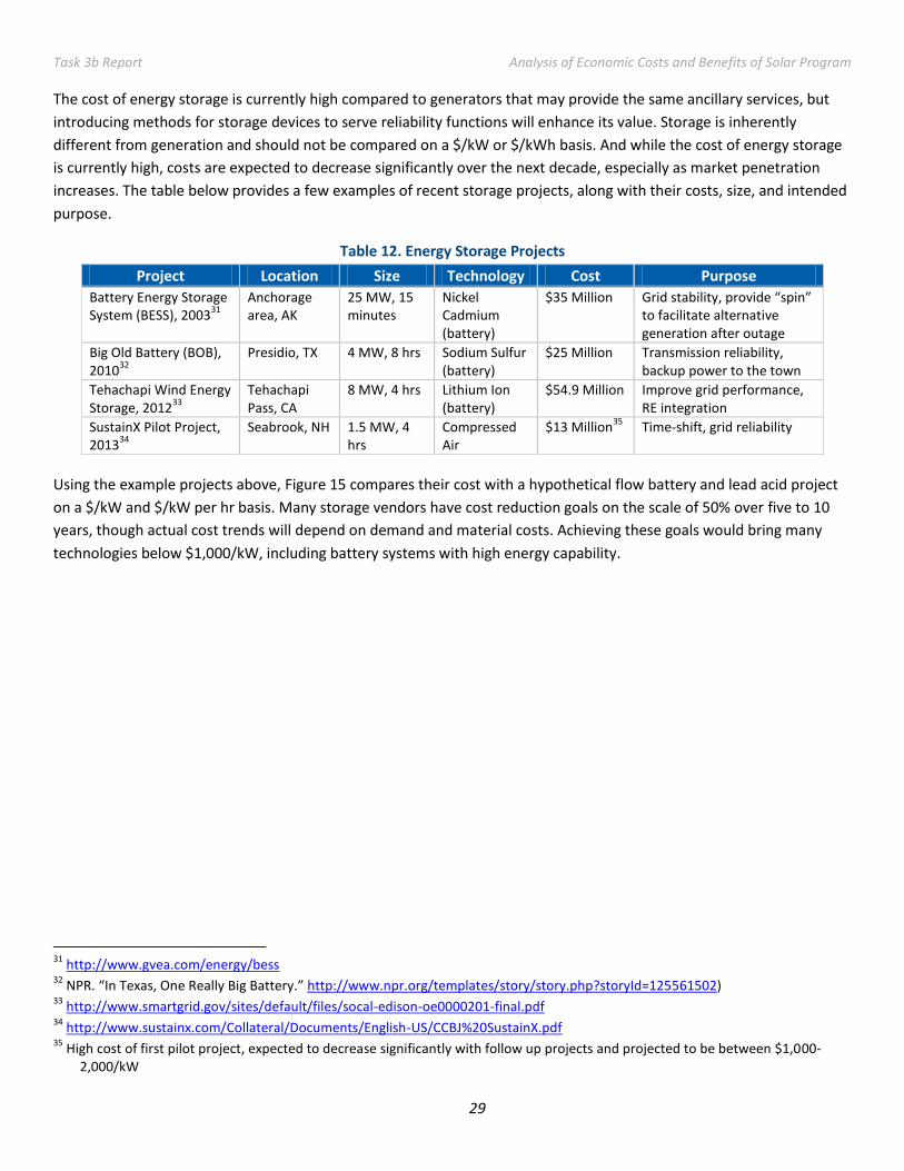
increases. The table below provides a few examples of recent storage projects, along with their costs, size, and intended
purpose.
Table 12. Energy Storage Projects
Project Location Size Technology Cost Purpose
Battery Energy Storage System (BESS), 2003
31
Anchorage area, AK
25 MW, 15 minutes
Nickel Cadmium (battery)
$35 Million Grid stability, provide “spin” to facilitate alternative generation after outage
Big Old Battery (BOB), 2010
32
Presidio, TX 4 MW, 8 hrs Sodium Sulfur (battery)
$25 Million Transmission reliability, backup power to the town
Tehachapi Wind Energy Storage, 2012
33
Tehachapi Pass, CA
8 MW, 4 hrs Lithium Ion (battery)
$54.9 Million Improve grid performance, RE integration
SustainX Pilot Project, 2013
34
Seabrook, NH 1.5 MW, 4 hrs
Compressed Air
$13 Million35
Time-shift, grid reliability
Using the example projects above, Figure 15 compares their cost with a hypothetical flow battery and lead acid project
on a $/kW and $/kW per hr basis. Many storage vendors have cost reduction goals on the scale of 50% over five to 10
years, though actual cost trends will depend on demand and material costs. Achieving these goals would bring many
technologies below $1,000/kW, including battery systems with high energy capability.
31
http://www.gvea.com/energy/bess 32
NPR. “In Texas, One Really Big Battery.” http://www.npr.org/templates/story/story.php?storyId=125561502) 33
http://www.smartgrid.gov/sites/default/files/socal-edison-oe0000201-final.pdf 34
http://www.sustainx.com/Collateral/Documents/English-US/CCBJ%20SustainX.pdf 35
High cost of first pilot project, expected to decrease significantly with follow up projects and projected to be between $1,000-2,000/kW

Task 3b Report Analysis of Economic Costs and Benefits of Solar Program
30
Figure 15. Project Cost Comparison36
Storage, Solar, and Microgrids Energy storage is an ideal technology for renewable energy integration because it can address the array of grid
integration challenges posed by variable generation: off-peak generation, requirements for new T&D capacity, need for
ancillary services, and other reliability impacts. Figure 16 depicts how storage could be used to balance out a system that
is entirely reliant on renewables. Hydro and biomass provide some baseload while wind generation fluctuates and often
exceeds load. Solar production occurs during peak hours, but it is not peak coincident. In total, renewables would be
under or over-generating at any given time without the usage of storage to keep things in balance.
36
Cost values for the hypothetical flow battery, lead acid, and flywheel projects are based on the following reference: Schoenung, Susan. “Energy Storage Systems Cost Update”. SANDIA National Labs. 4/2011 (SAND2011-2730)
-
1,000
2,000
3,000
4,000
5,000
6,000
7,000
8,000
9,000
10,000
$/kW $/kW per hr
($)
BESS
BOB
Tehachapi Project
Sustainx Pilot
Flow Battery (4hr)
Lead Acid (4hr)
Flywheel (15 min)

Task 3b Report Analysis of Economic Costs and Benefits of Solar Program
31
Figure 16. Hourly Supply and Demand, with Storage
The New England power grid has very high natural gas generation, which is ideal for ramping to follow changes in load
and variable generation. On the utility-scale, the challenges posed by large-scale renewables are focused around
transmission and distribution upgrades, ancillary services, and maintaining grid-wide reliability. As Massachusetts sees a
sharp rise in solar generation, utilities could employ energy storage technologies located on the system to address grid
reliability needs.
From a distributed generation standpoint, storage could alleviate these same challenges on a local scale, with benefits
attributed to both customers and the system. On a system with real time or dynamic pricing, solar production would be
worth more when shifted a few hours later to follow the load curve. Pairing storage with solar on the customer side
allows customers to be “islanded” from the grid.
Existing microgrid programs, such as the one in Connecticut, include microgrids of just one customer with backup
generation ranging from natural gas generators, fuel cells, or systems of solar, storage, and possibly a smaller generator.
It is also possible for multiple customers to share one storage system, though this is more easily implemented in
regulated utility territories where a utility installs one storage system for multiple customers to reduce their load
variability. If these customers install solar or other distributed generation (DG), the storage system could address
reliability issues before it affects the distribution grid.
Interest in microgrids has grown along with greater focus on both DG and grid modernization. Microgrids offer the
ability to enhance the DG asset, to lessen its burden on the grid, and allow the customer to island during outages or
faults. Table 13 lists the benefits of microgrid systems that accrue to the customer vs. the grid or system. One of the
challenges with storage is that the same storage project will provide benefits to multiple parties, but customers may be
asked to bear the entire cost of the storage project while not getting compensated for the grid benefits. Aside from high
costs, the storage industry has faced challenges from regulatory barriers that prevent one entity from capturing all
potential revenue streams for their investment.

Task 3b Report Analysis of Economic Costs and Benefits of Solar Program
32
Table 13. Customer Type and Grid/System
Customer Grid/System Provides backup power/ride-through capability Avoid high ramps in DG output, lowers system-wide
variability
Enables islanding during faults/outages Provide voltage/VAR support
Ability to shift production to capture higher peak prices
Ancillary Services
Lowers system peak demand
Looking forward With the roll-out of smart meters and enhanced communication and controls between utilities and customers, storage
on the customer side of the meter can provide more grid benefits than what is currently possible. As solar policies
continue to provide the incentives for customers to buy and install distributed solar, regulatory and policy support for
storage could lead to development of more storage and microgrid projects. If new grid technology enables customers to
provide and sell reliability services back to the grid, storage paired with solar could become an attractive investment.

Task 3b Report Analysis of Economic Costs and Benefits of Solar Program
33
Appendix A. Wholesale Market Price Forecast Key Assumptions
Market energy price projections are derived from the La Capra Associates Northeast Market Model (NMM). The La
Capra Associates NMM uses an hourly chronologic electric energy market simulation model based on the AURORAxmp®
software platform (AURORA). The model provides a zonal representation of the electrical system of New England and
the neighboring regions. For New England, the zones and corresponding transfer capabilities represented in the model
conform to the information provided in ISO New England’s Regional System Plan.
The underlying technology, AURORA, is a well-established, industry-standard simulation model that uses and captures
the effects of multiarea, transmission-constrained dispatch logic to simulate real market conditions. AURORA captures
the dynamics and economics of electricity markets.
The NMM utilizes a comprehensive database representing the entire Eastern Interconnect, including representations of
power generation units, zonal electrical demand, and transmission configurations. EPIS, the developer of AURORA,
provides a default database, which La Capra Associates supplements with updates to key inputs for the New England
market.
The NMM is used to develop a forecast that is representative of a 50/50 price outlook over the long-term. The reference
case assumptions for the 50/50 market price forecast are described in more detail below.
Retirement assumptions: The retirement assumptions are developed as part of the thermal expansion
development process. The schedule of retirements is based on both publicly announced retirements and the de-
list bids from the ISO-NE Forward Capacity Auctions (FCA). While submitting a de-list bid in advance and being
approved is not a guarantee that the unit will retire, using the FCA results provides for a retirement schedule
that is based on publicly-available market information that is not specific to any particular study. For years in
which no FCA had yet cleared, professional judgment was used to determine an expected life for the oil-fired
and coal-fired units remaining online in New England.
Natural Gas:
o Henry Hub: Prices are a blend of EIA’s May 2013 Short-Term Energy Outlook (2013-2015) and EIA’s 2013
Annual Energy Outlook (AEO) (2015 and after).
o New England Basis Differential: Basis differential is a blend of Algonquin City Gate Basis Swap Futures for the
short-term (2013-2015) and the implied basis differential from EIA’s 2013 AEO in the long-term (blended
until 2020 and fully from the 2013 AEO thereafter).
Carbon Policy/Price: All New England states participate in RGGI, a cap-and-trade program aimed at reducing CO2
emissions from the power sector. On February 7, 2013 the RGGI states announced their commitment to an
Updated Model Rule that would tighten the caps significantly in 2014. A RGGI-commissioned study of the
Updated Model Rule projects that emission allowance prices will rise from about $4 (2010$) per ton in 2014 to
over $10 (2010$) per ton by 2020.37 The NMM incorporates this updated outlook on RGGI allowance prices.
37
RGGI, Inc. 2/7/2013 Press Release. http://www.rggi.org/docs/PressReleases/PR130207_ModelRule.pdf

Task 3b Report Analysis of Economic Costs and Benefits of Solar Program
34
After 2020, the reference case assumes that a national CO2 pricing program is implemented and that prices will
reflect the “Low” case of Synapse Energy Economics, Inc.’s 2012 Carbon Dioxide Price Forecast.38
New Renewable Generation: For the renewable build-out, it was assumed that the RPS programs would
continue throughout the study period and developed a build-out that included enough renewable energy to
meet the current targets each year. Most of the states’ required percentages stop increasing at some point in
the study period, after this additional build-out is based on maintaining the percentage target as load increases.
For example, the Connecticut RPS requirement increases each year to 20% by 2020, for 2021 and beyond we
assume that Connecticut will require additional renewables to maintain the 20% requirement as load grows. The
Massachusetts requirement is assumed to continue to grow 1% per year through 2031 to 26%; after that we
maintain the 26% requirement and additional renewables required are due to load growth. We assumed that
imports from New York would start at 1125 GWh in 2013 and increase to 1800 GWh by 2018. Imports from
Canada were assumed to be fixed at 717 GWh per year. Finally, the production tax credit (PTC) was phased out
on the schedule similar to one proposed by the American Wind Energy Association (AWEA). The PTC is assumed
to be 100% of its current level through 2014 and decreasing between 2015 and 2019, as shown in the table
below.
2014 2015 2016 2017 2018 2019 and
Beyond
100% 80% 70% 60% 60% 0%
Inflation: The NMM uses the GDP Chain-type Price Index from the Macroeconomic Indicators table of the 2013
AEO.
Load and DSM: The 2013 CELT report was used to estimate gross peak and energy load and peak and energy
load net of energy efficiency (EE) for the first ten years of the study period. For later years, gross load is assumed
to grow at the 2016-2021 compound annual growth rate. EE reductions are extrapolated such that EE’s percent
of gross load, both peak and energy, in 2021 remains constant through the rest of the study period. These
extrapolations are done separately for each zone in the system.
Transmission: The NMM assumes the following upgrades to the existing New England transmission system:
o The Maine Power Reliability Project (Completed by 2013),
o Northern Pass (Completed by 2019), and
o New England East-West Solution (Greater Springfield Reliability Project completed by 2014,
o Interstate Reliability Project completed by 2016).
38
Synapse, http://www.synapse-energy.com/Downloads/SynapseReport.2012-10.0.2012-CO2-Forecast.A0035.pdf