task 2 - physical hardening of binders and mixtures task 3

Task 2 - Physical Hardening of Binders and Mixtures

Raul Velasquez Hassan Tabatabaee Hussain Bahia 10/05/2011

Low Temperature

Pooled Fund Study

Phase II

Task 5 - Modeling Asphalt Mixtures Contraction- Expansion

Task 3 - Development of the Single-Edge Notched Beam (SENB) Test

Objectives Task 2

1. Develop method to simplify measurements of physical hardening

2. Model to adjust Stiffness and m-value based on climatic condition

3. Collect physical hardening for variety of asphalt binders

4. Use Tg to quantify effect of isothermal storage on dimensional stability of asphalt mixtures

5. Effect of PPA, WMA additives, and Polymers on physical hardening

Physical hardening (aging)- Not a new topic

• It is caused by time dependent isothermal

changes in specific volume.

• It is similar to reducing temperature.

• Effect completely removed when material is heated

to room temperatures.

• Physical hardening for polymers can be

explained by free volume theory in Glass

Transition region (Struik (1978) and Ferry (1980))

Physical Hardening Model For Asphalt Binders (1) and (2)

• Mechanism of gradual particle rearrangement toward lower free volume,

resulting in gradual increase in stiffness, can be described as a “creep”

behavior.

• In which:

– ϵPH is isothermal contraction

– ΔS/S0 is the hardening rate

– T0 is the peak temperature for hardening rate, assumed to be the Tg (

C)

– T is the conditioning temperature (

C)

– tc is the conditioning time (hrs)

– 2x is the length of the temperature range of the glass transition region (

C)

– G and η are model constants, derived by fitting the model

Temp dependant “stress” term

Kelvin-Voigt Model Structure

Physical Hardening and Temperature

•Physical hardening for 40 binders investigated:

– Physical hardening was small at T >> Tg

– Physical hardening peaked at T ≈ Tg

– In half of binders, physical hardening was less at Tc < Tg

0.10

0.20

0.30

0.40

0.50

0.60

-25 -15 -5 5 15 25

Ha

rden

ing

Ra

te a

t 2

4 h

rs (

-)

T-Tg (

C)

Binder 1 Binder 2 Binder 3 Binder 4 Binder 5

(Planche et al., 1998)

Specific

Volume

Temperature Glass Transition

Temperature (Tg)

0

0.2

0.4

0.6

0.8

1

1.2

-60 -55 -50 -45 -40 -35 -30 -25 -20 -15 -10 -5 0x x

Temp dependant “stress” term

Physical Hardening Model (1) and (2)

• Physical hardening is limited to glass transition region

• Physical hardening Rate peaks at Tg

(Hardening rate= ∆S/S0)

Obtaining parameters of physical hardening model (2)

First approach:

1. Run BBR test for sample at 3 conditioning times (i.e. 1, 3, and 6 hrs, or longer!)

2. Use Glass Transition temperature (Tg) and length of Tg region from binder Tg test.

The longer the test duration, higher the accuracy

Second approach: 1. Run BBR test at 1 hr conditioning time at 3

temperatures, as in performance grading 2. Calculate power law slope, B. 3. Use B along with Tg and length of Tg region from

glass transition test to predict model parameters G and η

G and η are unique for every binder, thus constant at all

conditioning times and temperatures Tg may be indirectly estimated from BBR conditioning

tests at 3 temperatures

Obtaining parameters of physical hardening model (2)

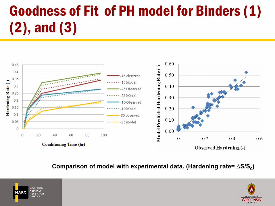
Goodness of Fit of PH model for Binders (1) (2), and (3)

Comparison of model with experimental data. (Hardening rate= ∆S/S0)

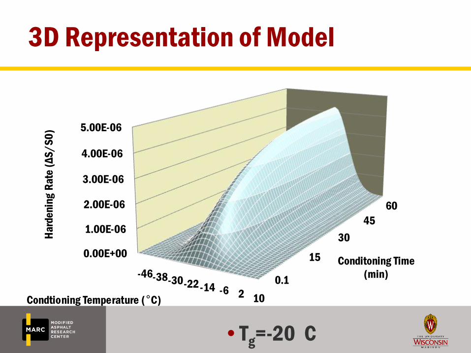
3D Representation of Model

•Tg=-20

C

102-6-14-22-30-38-46

0.00E+00

1.00E-06

2.00E-06

3.00E-06

4.00E-06

5.00E-06

0.1

15

30

45

60

Condtioning Temperature ( C)

Ha

rde

nin

g R

ate

(Δ

S/

S0

)

Conditoning Time

(min)

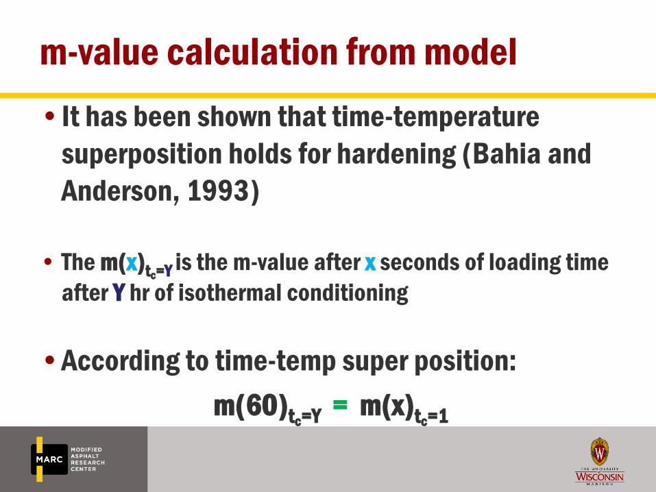
m-value calculation from model

•It has been shown that time-temperature

superposition holds for hardening (Bahia and

Anderson, 1993)

• The m(x)tc=Y is the m-value after x seconds of loading time

after Y hr of isothermal conditioning

•According to time-temp super position:

m(60)tc=Y = m(x)tc=1

2.50

2.60

2.70

2.80

2.90

3.00

3.10

0.00 0.50 1.00 1.50 2.00 2.50

Log

S

Loading time (Sec)

AAB1 Observed Log S at -25 1hr

AAB1 Modeled Log S at -25 6hr



superpositioned curve

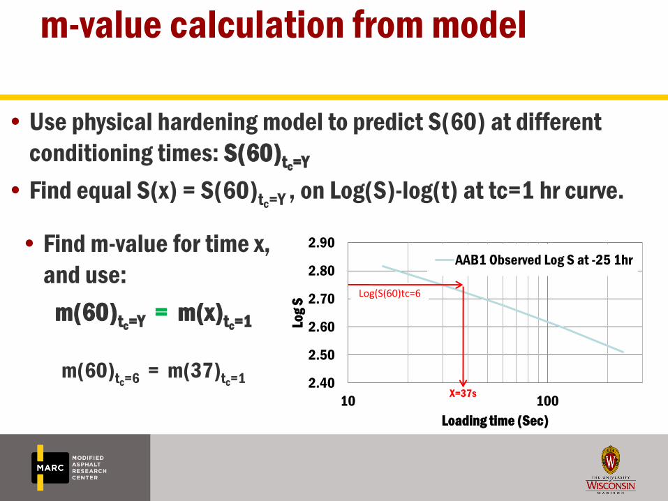
• Use physical hardening model to predict S(60) at different

conditioning times: S(60)tc=Y

• Find equal S(x) = S(60)tc=Y , on Log(S)-log(t) at tc=1 hr curve.


2.40

2.50

2.60

2.70

2.80

2.90

10 100

Log

S

Loading time (Sec)

AAB1 Observed Log S at -25 1hr

X=37s

Log(S(60)tc=6

• Find m-value for time x,

and use:

m(60)tc=Y = m(x)tc=1

m(60)tc=6 = m(37)tc=1


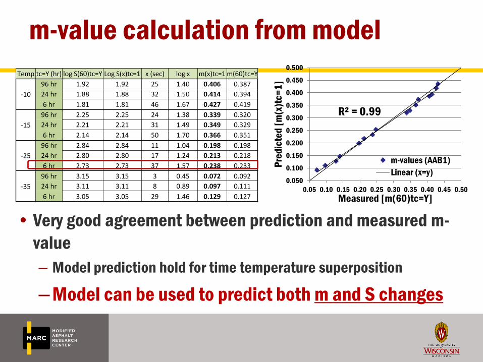
Temp tc=Y (hr) log S(60)tc=Y Log S(x)tc=1 x (sec) log x m(x)tc=1 m(60)tc=Y

-10

96 hr 1.92 1.92 25 1.40 0.406 0.387

24 hr 1.88 1.88 32 1.50 0.414 0.394

6 hr 1.81 1.81 46 1.67 0.427 0.419

-15

96 hr 2.25 2.25 24 1.38 0.339 0.320

24 hr 2.21 2.21 31 1.49 0.349 0.329

6 hr 2.14 2.14 50 1.70 0.366 0.351

-25

96 hr 2.84 2.84 11 1.04 0.198 0.198

24 hr 2.80 2.80 17 1.24 0.213 0.218

6 hr 2.73 2.73 37 1.57 0.238 0.233

-35

96 hr 3.15 3.15 3 0.45 0.072 0.092

24 hr 3.11 3.11 8 0.89 0.097 0.111

6 hr 3.05 3.05 29 1.46 0.129 0.127

R² = 0.99

0.050

0.100

0.150

0.200

0.250

0.300

0.350

0.400

0.450

0.500

0.05 0.10 0.15 0.20 0.25 0.30 0.35 0.40 0.45 0.50

Pre

dic

ted

[m

(x)t

c=1

]

Measured [m(60)tc=Y]

m-values (AAB1)

Linear (x=y)

• Very good agreement between prediction and measured m-

value

– Model prediction hold for time temperature superposition

–Model can be used to predict both m and S changes

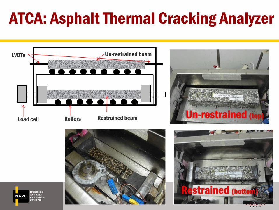
ATCA: Asphalt Thermal Cracking Analyzer

Load cell Rollers Restrained beam

Un-restrained beam LVDTs

Un-restrained (top)

Restrained (bottom)

ATCA System: Sample preparation

TSRST

Sample

Preparation:

ATCA=>Quantify effect of isothermal storage

on dimensional stability of asphalt mixtures (4)

The ATCA can simultaneously test two asphalt mixture

beams under following conditions:

– unrestrained specimen from which change in length with

temperature is measured

– restrained specimen to measure thermal stress buildup.

– Both specimens produced from same sample and both exposed to

same thermal history

0.0

0.2

0.4

0.6

0.8

1.0

1.2

1.4

1.6

1.8

2.0

0 50 100 150 200 250Time (min)

Stre

ss (

MP

a)

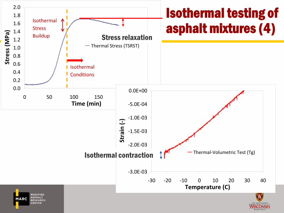
Thermal Stress (TSRST)

Stress relaxation

Isothermal

Conditions

Isothermal

Stress

Buildup

-3.0E-03

-2.5E-03

-2.0E-03

-1.5E-03

-1.0E-03

-5.0E-04

0.0E+00

-30 -20 -10 0 10 20 30 40Temperature (C)

Stra

in (

-)

Thermal-Volumetric Test (Tg)Isothermal contraction

Isothermal testing of asphalt mixtures (4)

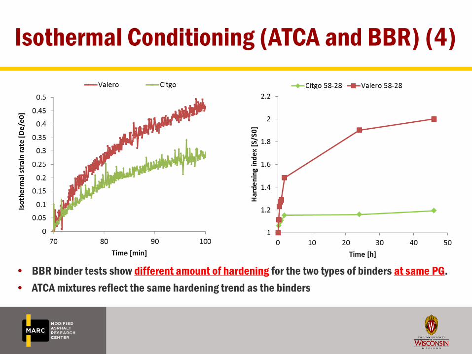
Isothermal Conditioning (ATCA and BBR) (4)

• BBR binder tests show different amount of hardening for the two types of binders at same PG.

• ATCA mixtures reflect the same hardening trend as the binders

Effect of Cooling Rate

• Delayed strain during fast cooling takes place isothermally

• If enough isothermal time is given, mixes reach same stress level

Isothermal

Stress

Buildup

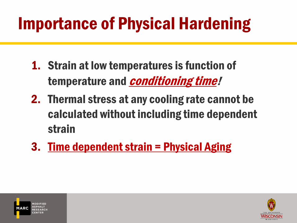
Importance of Physical Hardening

1. Strain at low temperatures is function of

temperature and conditioning time!

2. Thermal stress at any cooling rate cannot be

calculated without including time dependent

strain

3. Time dependent strain = Physical Aging

Importance of Physical Hardening

Isothermal Stress Build-up

Fracture

MN County Road 112-CITGO restrained

beam fracture under isothermal conditions

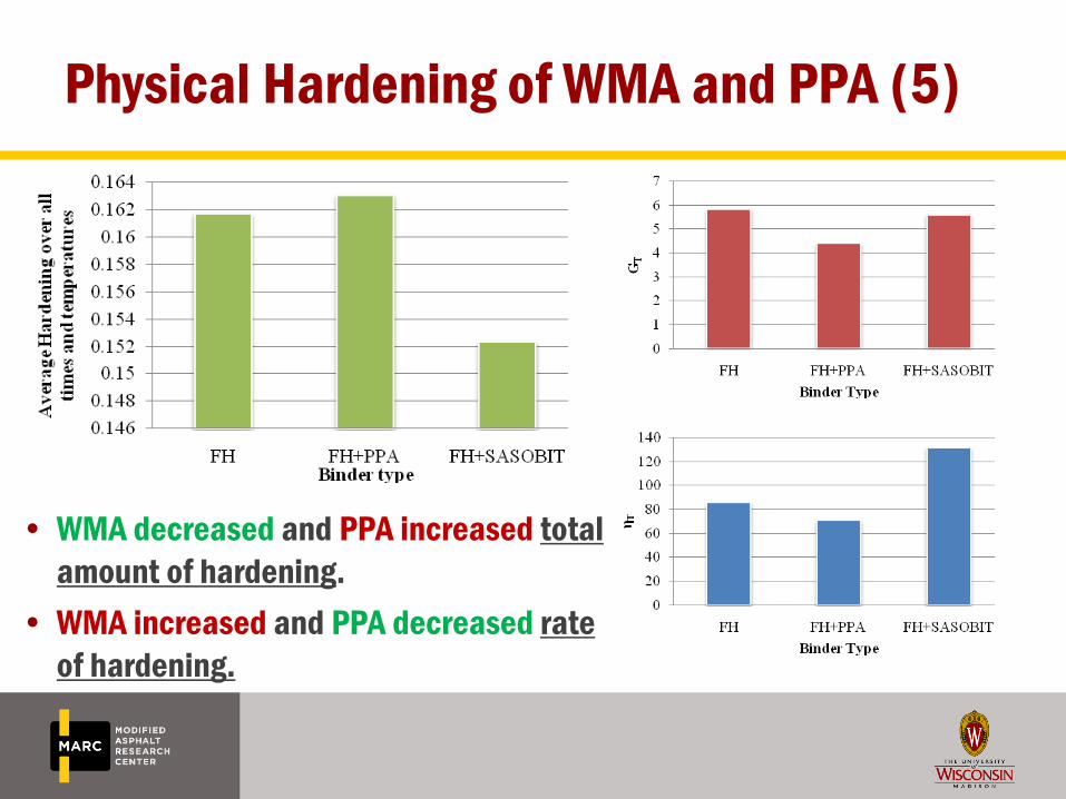
Physical Hardening of WMA and PPA (5)

• WMA decreased and PPA increased total

amount of hardening.

• WMA increased and PPA decreased rate

of hardening.

Conclusions Task 2

• Physical hardening in asphalt binders results in significant

changes in their creep response at temperatures below or near

glass transition

• Physical hardening can be represented with “creep” model with

parameters obtained from BBR and/or Tg tests

• Thermal stress calculations are not accurate without

accounting for Glass Transition and time-dependant strain

(isothermal contraction)

• Effect of isothermal contraction becomes very important when

using lab tests at faster cooling rates to predict field conditions

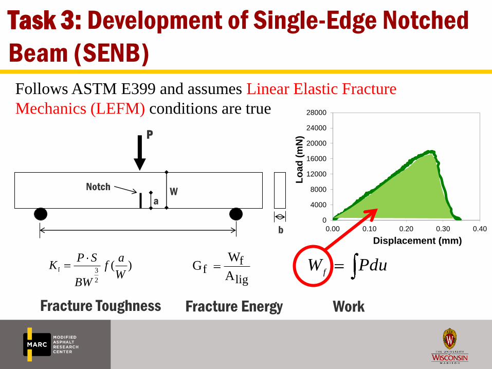
Task 3: Development of Single-Edge Notched

Beam (SENB)

b

P

W a

Notch

3

2

( )P S a

K fW

BW

Follows ASTM E399 and assumes Linear Elastic Fracture

Mechanics (LEFM) conditions are true

lig

ff

A

WG PduW

f

Fracture Toughness Fracture Energy Work

0

4000

8000

12000

16000

20000

24000

28000

0.00 0.10 0.20 0.30 0.40

Lo

ad

(m

N)

Displacement (mm)

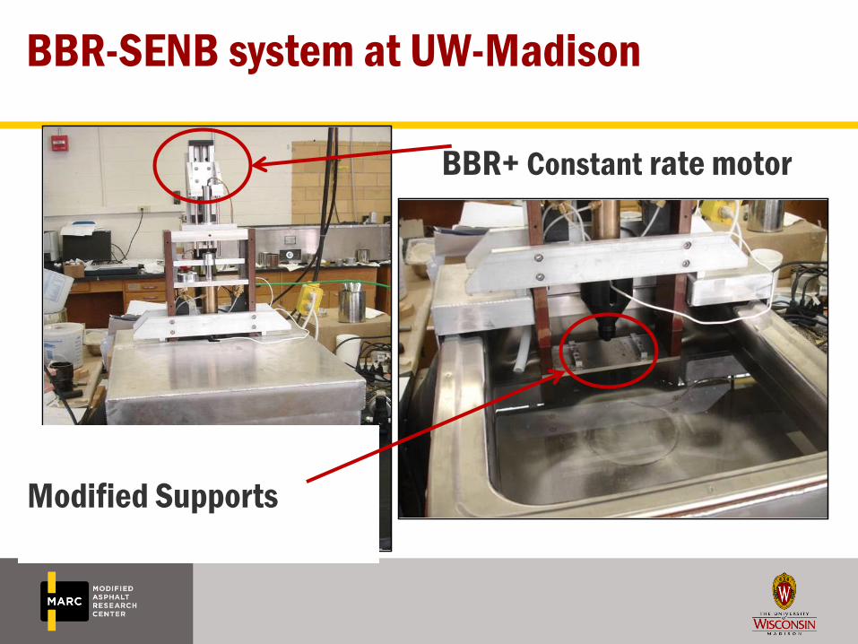
BBR-SENB system at UW-Madison

Modified Supports

BBR+ Constant rate motor

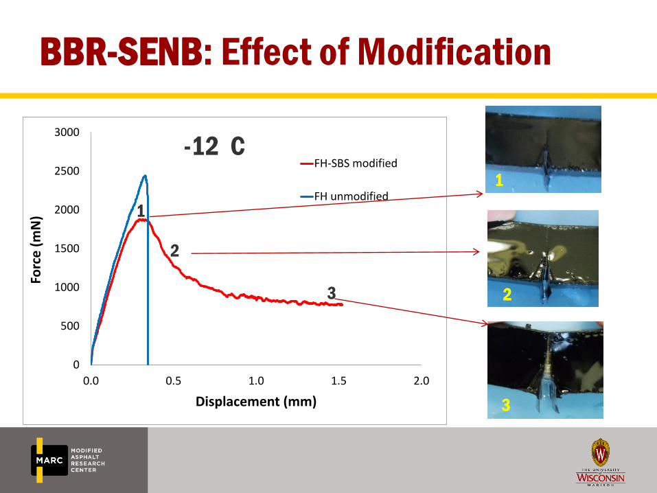
BBR-SENB: Effect of Modification

0

500

1000

1500

2000

2500

3000

0.0 0.5 1.0 1.5 2.0

Forc

e (

mN

)

Displacement (mm)

FH-SBS modified

FH unmodified

1

2

3

1

2

3

-12

C

R² = 0.25

0

10

20

30

40

50

60

70

80

0.2 0.3 0.4 0.5 0.6

Gf

(J/m

2)

m(60) (-)

-12 C -18 C -24 C

R² = 0.17

0

10

20

30

40

50

60

70

80

0.2 0.3 0.4 0.5 0.6

KIC

(K

Pa.

m0

.5)

m(60) (-)

-12 C -18 C -24 C

SENB vs. BBR

• BBR m-value and creep stiffness have very poor correlation with the SENB

parameters.

• BBR criteria fails to account for many binders with low fracture energy.

SENB vs. BBR

R² = 0.37

0

10

20

30

40

50

60

70

80

0 100 200 300 400 500 600 700

Gf

(J/m

2)

S(60) (MPa)

-12 C -18 C -24 C

R² = 0.10

0

10

20

30

40

50

60

70

80

0 100 200 300 400 500 600 700

KIC

(K

Pa.

m0

.5)

S(60) (MPa)

-12 C -18 C -24 C

SENB fracture energy (Gf) clearly discriminates between binders with similar stiffness and m-value.

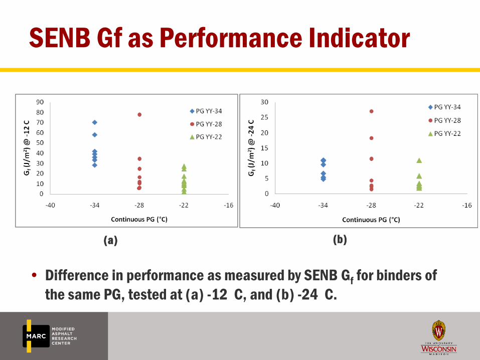
SENB Gf as Performance Indicator

• Difference in performance as measured by SENB Gf for binders of

the same PG, tested at (a) -12

C, and (b) -24

C.

(a) (b)

Brittle-Ductile Transition

• KIC does not show a clear trend above and below TG.

• Gf decreases at temps below TG.

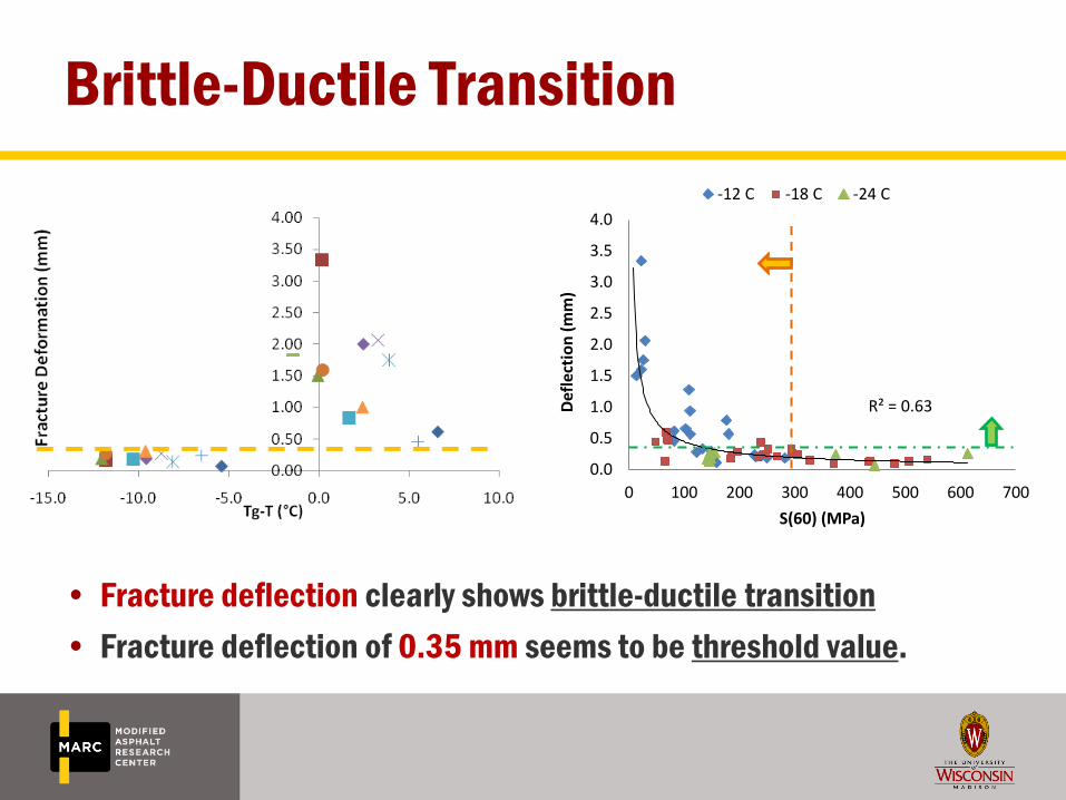
R² = 0.63

0.0

0.5

1.0

1.5

2.0

2.5

3.0

3.5

4.0

0 100 200 300 400 500 600 700

Def

lect

ion

(m

m)

S(60) (MPa)

-12 C -18 C -24 C

• Fracture deflection clearly shows brittle-ductile transition

• Fracture deflection of 0.35 mm seems to be threshold value.

Brittle-Ductile Transition

SENB vs LTPP Data

90961 (9.3)

• Lower TC index shows better low temp performance

• Binders with lower TC Index have higher Gf and failure deflection

TC Index: # of Thermal Cracks/Freeze Index

LTPP ID code

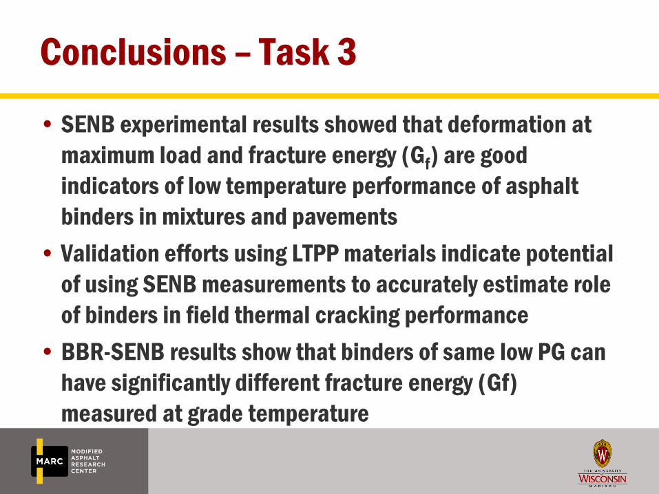
Conclusions – Task 3

• SENB experimental results showed that deformation at

maximum load and fracture energy (Gf) are good

indicators of low temperature performance of asphalt

binders in mixtures and pavements

• Validation efforts using LTPP materials indicate potential

of using SENB measurements to accurately estimate role

of binders in field thermal cracking performance

• BBR-SENB results show that binders of same low PG can

have significantly different fracture energy (Gf)

measured at grade temperature

Objectives Task 5

1. Expand database of thermo-volumetric properties of asphalt binders and mixtures

2. Develop micromechanics-numerical model to estimate glass transition and coefficient of thermal expansion of mixtures from properties of binder and aggregate

3. Conduct thermal cracking sensitivity to determine which of glass transition parameters are statistically important

Mixture and Binder TG measurements (1)

-1.2

-1

-0.8

-0.6

-0.4

-0.2

0

0.2

-80 -60 -40 -20 0 20 40

Len

gth

Ch

ange

(m

m)

Dummy temperature [°C]

Cell 35 (Mixture)

Cell 20 (Mixture)

-10

0

10

20

30

40

-40 -20 0 20 40

Vo

lum

e ch

ange

[m

m3

/mm

3]

Dummy temperature [°C]

Cell 20 (Binder)

Cell 35 (Binder)

= c + g(T – Tg) + R( l – g) ln{1 + exp[(T – Tg)/R]}

Database of thermo-volumetric

measurements extended

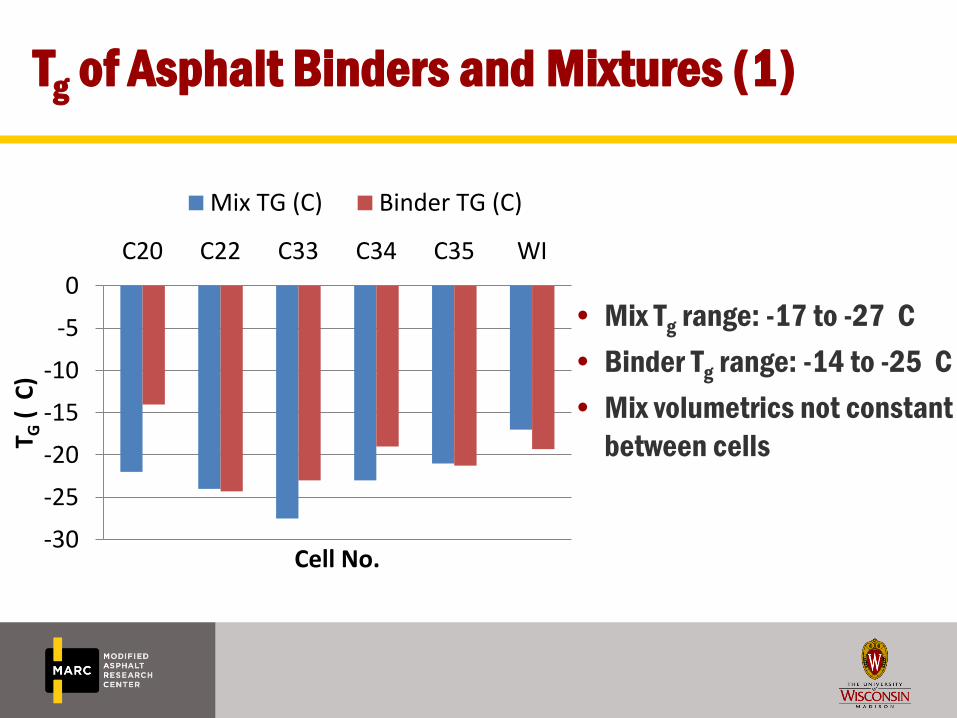
• Mix Tg range: -17 to -27

C

• Binder Tg range: -14 to -25

C

• Mix volumetrics not constant

between cells

-30

-25

-20

-15

-10

-5

0

C20 C22 C33 C34 C35 WI

T G (

C

)

Cell No.

Mix TG (C) Binder TG (C)

Tg of Asphalt Binders and Mixtures (1)

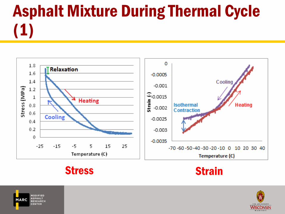
Asphalt Mixture During Thermal Cycle (1)

Stress Strain

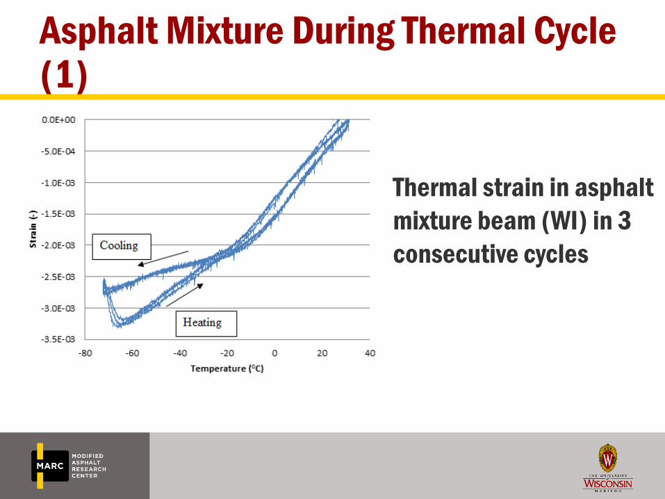
Asphalt Mixture During Thermal Cycle (1)

Thermal strain in asphalt

mixture beam (WI) in 3

consecutive cycles

Stress curves under thermal cycling and isothermal conditioning for MnROAD Cell 33

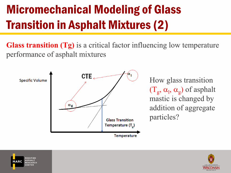
Micromechanical Modeling of Glass

Transition in Asphalt Mixtures (2)

Glass transition (Tg) is a critical factor influencing low temperature

performance of asphalt mixtures

How glass transition

(Tg, l, g) of asphalt

mastic is changed by

addition of aggregate

particles?

Motivation for development of micromechanical

model for prediction of CTEs (2)

• Existing models for thermal cracking predictions over- simplify thermo-volumetric properties of AC

• Glass transition and coefficient of thermal expansion/contraction of mixtures above and below Tg needed for accurate prediction of thermal stresses

TOTAL

AGGAGGbinderMIX

V

VVMAL

3Currently in MEPDG

Internal Structure of AC: Digital Image Analysis

Scanned images of AC are converted to black

and white (BW) images

BW images are matrixes of 0 (mastic) and 1

0 (aggregate)

iPas => Matlab based program to calculate

aggregate proximity index (API), aggregate

orientation, “contact” length, API in branches,

# of branches Developed in collaboration

with Prof. Kutay from MSU

Input Image

Intensity Distribution

181

0 255

Thresholded Black and white image

Input Image


176

0 255

12

3

4

5

6

7

8

9

10

11

12

13

14

15

16

17

18

19

20

Input Image


176

0 255

12

3

4

5

6

7

8

9

10

11

12

13

14

15

16

17

18

19

20

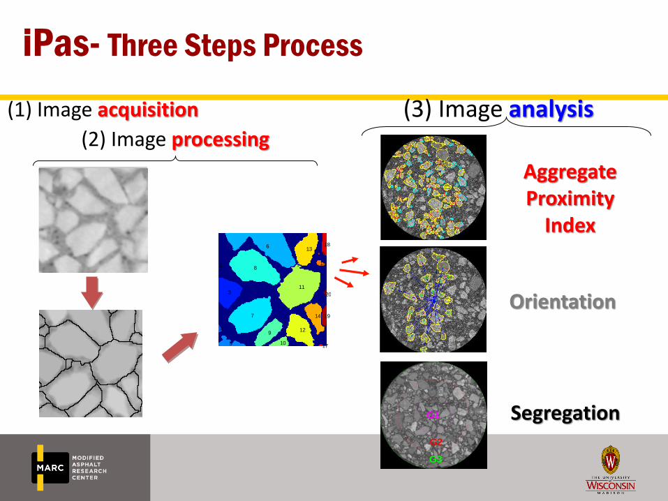
(2) Image processing

(3) Image analysis

Aggregate Proximity

Index

Orientation

Segregation G1

G2

G3

iPas- Three Steps Process

(1) Image acquisition

Aggregate Proximity Index (API)=> “contact points”

Minimum aggregate size & surface distance threshold needs to be

defined for Aggregate Proximity Index (API) estimation

Other internal structural parameters

“Contact” Length

Aggregate Branches-

Connectivity

Contact Orientation

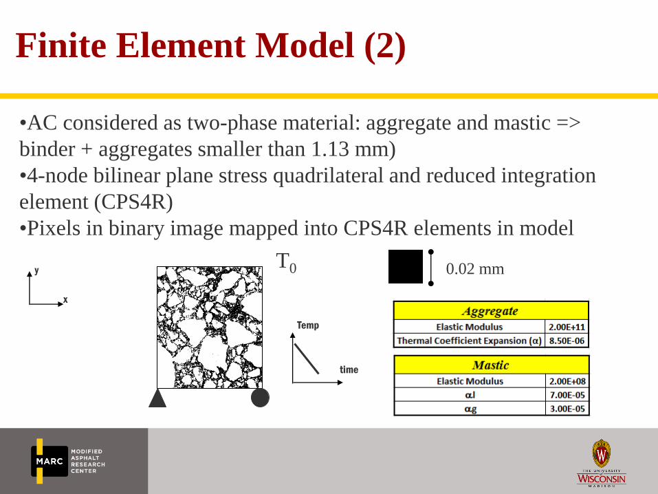
Finite Element Model (2)

•AC considered as two-phase material: aggregate and mastic =>

binder + aggregates smaller than 1.13 mm)

•4-node bilinear plane stress quadrilateral and reduced integration

element (CPS4R)

•Pixels in binary image mapped into CPS4R elements in model

y

x

0.02 mm T0

Temp

time

Finite Element Model Input (2)

Mixes with

different

gradations

0

10

20

30

40

50

60

70

80

90

100

0.01 0.1 1 10 100

% P

ass

ing

Sieve Size (mm)

Mix 5

Mix 1 & 3

Mix 2 & 4

Superpave Limits

Thermo-Volumetric Response of AC

0.00

0.02

0.04

0.06

0.08

0.10

0.12

0.14

-60 -40 -20 0

The

rma

l Str

ain

(%

)

Temperature (

C)

High connectivity

Low connectivity

0.00

0.05

0.10

0.15

0.20

0.25

0.30

0.35

-70 -60 -50 -40 -30 -20 -10 0 10 20 30 40

Str

ain

(%

)

Temperature (°C)

Tg ≈ -14 C

Typical measured

FE simulation

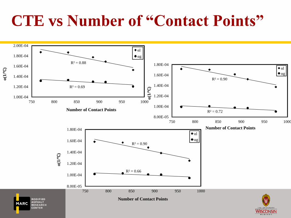
CTE vs Number of “Contact Points”

R² = 0.88

R² = 0.69

1.00E-04

1.20E-04

1.40E-04

1.60E-04

1.80E-04

2.00E-04

750 800 850 900 950 1000

α(1

/℃)

Number of Contact Points

αl

αg

R² = 0.90

R² = 0.72

8.00E-05

1.00E-04

1.20E-04

1.40E-04

1.60E-04

1.80E-04

750 800 850 900 950 1000

α(1

/℃)


αl

αg

R² = 0.90

R² = 0.66

8.00E-05

1.00E-04

1.20E-04

1.40E-04

1.60E-04

1.80E-04

750 800 850 900 950 1000

α(1

/℃)


αl

αg

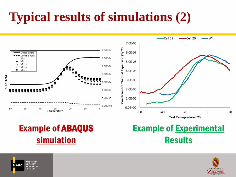
Typical results of simulations (2)

0.0E+00

1.0E-05

2.0E-05

3.0E-05

4.0E-05

5.0E-05

6.0E-05

7.0E-05

-60 -40 -20 0 20

Co

effi

cien

t o

f Th

erm

al E

xpan

sio

n (

1/°

C)

Test Temeprature (°C)

Cell 22 Cell 20 WI

Example of ABAQUS

simulation

Example of Experimental

Results

Proposed Semi-empirical Micromechanics Model for CTE (2)

Based on the commonly used Hirsch model for estimation of

modulus of asphalt mixes.

•

and

are arithmetic mean of CTE of mastic and aggregate

•

and

are harmonic mean of CTE of mastic and aggregate, which is a

function of stiffness ratio ( Emastic/E aggregate)

• F is an empirical function of mastic stiffness and aggregate contact points (internal

structure)

Validation of model for CTE (2)

To validate model=> 9 different mixtures which

have different aggregate structures and mastic

properties have been used

R² = 0.96

y = x

5.00E-05

1.00E-04

1.50E-04

2.00E-04

2.50E-04

5.00E-05 1.00E-04 1.50E-04 2.00E-04 2.50E-04

αl ev

alu

ate

d f

rom

th

e S

imu

lati

on

(1/℃

)

αl evaluated from the model (1/℃)

R² = 0.88

y = x

6.00E-05

9.00E-05

1.20E-04

1.50E-04

1.80E-04

6.00E-05 9.00E-05 1.20E-04 1.50E-04 1.80E-04

αg e

va

lua

ted

fro

m t

he

Sim

ula

tion

(1/℃

)

αg evaluated from the model (1/℃)

Thermal Cracking Sensitivity to Thermo-volumetric parameters (3)

Run 1 Run 2 Run 3 Run 4 Run 5 Run 6 Run 7 Run 8 Run 9 Run 10 Run 11 Run 12 Run 13 Run 14 Run 15 Run 16 Run 17

Coolin

g

Tg -17 -20 -13 -17 -17 -17 -17 -17 -17 -17 -17 -17 -17 -17 -17 -17 -17

R 6 6 6 7 5 6 6 6 6 6 6 6 6 6 6 6 6

αl 5E-5 5E-5 5E-5 5E-5 5E-5 6E-5 4E-5 5E-5 5E-5 5E-5 5E-5 5E-5 5E-5 5E-5 5E-5 5E-5 5E-5

αg 1E-5 1E-5 1E-5 1E-5 1E-5 1E-5 1E-5 1.3E-5 9E-6 1E-5 1E-5 1E-5 1E-5 1E-5 1E-5 1E-5 1E-5

Hea

ting

Tg -17 -17 -17 -17 -17 -17 -17 -17 -17 -20 -13 -17 -17 -17 -17 -17 -17

R 6 6 6 6 6 6 6 6 6 6 6 7 5 6 6 6 6

αl 5E-5 5E-5 5E-5 5E-5 5E-5 5E-5 5E-5 5E-5 5E-5 5E-5 5.E-5 5.E-5 5.E-5 6E-5 4E-5 5.E-5 5.E-5

αg 1E-5 1E-5 1E-5 1E-5 1E-5 1E-5 1E-5 1E-5 1E-5 1E-5 1E-5 1E-5 1E-5 1E-5 1E-5 1.3E-5 9E-6

• Analysis matrix was designed to systematically vary thermo-volumetric

parameters in cooling and heating

• Thermal stress model from Tabatabaee et al., 2012 (submitted to TRB)

used.

• Model accounts for thermo-volumetric parameters in cooling and

heating and effect of physical hardening.

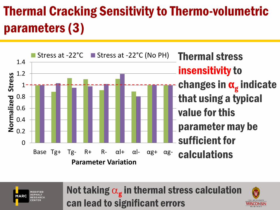
Thermal Cracking Sensitivity to Thermo-volumetric

parameters (3)

0

0.2

0.4

0.6

0.8

1

1.2

1.4

Base Tg+ Tg- R+ R- αl+ αl- αg+ αg-

No

rmal

ize

d S

tre

ss

Parameter Variation

Stress at -22°C Stress at -22°C (No PH) Thermal stress

insensitivity to

changes in αg indicate

that using a typical

value for this

parameter may be

sufficient for

calculations

Not taking g in thermal stress calculation

can lead to significant errors

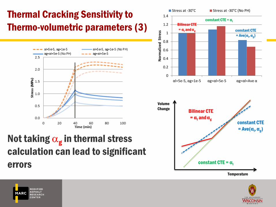
Thermal Cracking Sensitivity to

Thermo-volumetric parameters (3)

0

0.2

0.4

0.6

0.8

1

1.2

1.4

αl=5e-5, αg=1e-5 αg=αl=5e-5 αg=αl=Ave α

No

rmal

ize

d S

tres

s

Stress at -30°C Stress at -30°C (No PH)

Bilinear CTE

= αl and αg constant CTE

= Ave(αl, αg)

constant CTE = αl

Not taking g in thermal stress

calculation can lead to significant

errors constant CTE = αl

constant CTE

= Ave(αl, αg)

Bilinear CTE

= αl and αg

Temperature

Volume

Change

Conclusions – Task 5

• Thermo-volumetric behavior of AC can not be described

only with volumetric information of constituents

• Information about internal structure of AC needs to be

included in estimation of CTE

• Glass transition temperature of Binder is very similar to

Mixture

• When taking into account Physical Hardening, thermal

stress calculation is sensitive to: l, Tg, width of Tg region

(R)

task 2 - physical hardening of binders and mixtures task 3

Documents