Taking Stock:A Rigorous Modelling of Animal Spirits

in Macroeconomics

Reiner Franke∗ and Frank Westerhoff

University of Kiel (GER) and University of Bamberg (GER)

December 2016

Abstract

This paper is a survey of the burgeoning literature that seeks to take the enig-matic concept of the animal spirits more seriously by building heterodox mac-rodynamic models that can capture some of its crucial aspects in a rigorousway. Two approaches are considered: the discrete choice and the transi-tion probability approach, where individual agents face a binary decision andchoose one of them with a certain probability. These assessments are adjustedupward or downward in response to what the agents observe, which leads tochanges in the aggregate sentiment and the macroeconomic variables resultingfrom the corresponding decisions. Typical applications of the two approachesalternatively give rise to what will be called a weak and a strong form ofanimal spirits. On the whole, the literature included in this survey providesexamples of applications of a modelling tool that demonstrates a considerableflexibility within a canonical framework.

JEL classification: C 02, D84, E12, E30.

Keywords: Business sentiment, discrete choice approach, transition probabil-ity approach, cyclical behaviour, estimation.

∗Corresponding author, email: franke@uni-bremen.de .

1 Introduction

A key issue in which heterodox macroeconomic theory differs from the orthodoxy isthe notion of expectations, where it determinedly abjures the Rational ExpectationsHypothesis. Instead, to emphasize its view of a constantly changing world with itsfundamental uncertainty, heterodox economists frequently refer to the famous ideaof the ‘animal spirits’. This is a useful keyword that poses no particular problemsin general conceptual discussions. However, given the enigma surrounding the ex-pression, what can it mean when it comes to rigorous formal modelling? Moreoften than not, authors garland their model with this word, even if there may beonly loose connections to it. The present survey focusses on heterodox approachesthat take the notion of the ‘animal spirits’ more seriously and, seeking to learn moreabout its economic significance, attempt to design dynamic models that are able todefinitively capture some of its crucial aspects.1

The background of the term as it is commonly referred to is Chapter 12 ofKeynes’ General Theory, where he discusses another elementary “characteristic ofhuman nature,” namely, “that a large proportion of our positive activities depend onspontaneous optimism rather than on a mathematical expectation” (Keynes, 1936,p. 161). Although the chapter is titled “The state of long-term expectation”, Keynesmakes it clear that he is concerned with “the state of psychological expectation”(p. 147).2

It is important to note that this state does not arise out of the blue from whimsand moods; it is not an imperfection or plain ignorance of human decision-makers.Ultimately, it is due to the problem that decisions resulting in consequences thatreach far into the future are not only complex, but also fraught with irreducibleuncertainty. “About these matters”, Keynes wrote elsewhere to clarify the basicissues of the General Theory, “there is no scientific basis on which to form anycalculable probability whatever” (Keynes, 1937, p. 114). Needless to say, this facetof Keynes’ work is completely ignored by the “New-Keynesian” mainstream.

To cope with uncertainty that cannot be reduced to a mathematical risk cal-culus, enabling us nevertheless “to behave in a manner which saves our faces as

1The term is so appealing that a number of orthodox economists also invoke it to advertise theirmodels. In a branch of the Dynamic Stochastic General Equilibrium literature, the term is usedinterchangeably with sunspot equilibria and self-fulfilling prophecies. It goes without saying thatthe discussion in the present paper has nothing to do with these (very elaborate) refinements ofrational expectations, where observations of an exogenous stochastic process induce the agents tocoordinate on recurrent switches between multiple equilibria; see, for example, Farmer and Guo(1994), and Galı (1994).

2The actual term ‘animal spirits’ is mentioned in the same chapter on p. 161.

1

rational economic men” (ibid.), Keynes refers to “a variety of techniques”, or “prin-ciples”, which are worth quoting in full.

“(1) We assume that the present is a much more serviceable guide tothe future than a candid examination of past experience would show itto have been hitherto. In other words we largely ignore the prospect offuture changes about the actual character of which we know nothing.

“(2) We assume that the existing state of opinion as expressed in pricesand the character of existing output is based on a correct summing upof future prospects, so that we can accept it as such unless and untilsomething new and relevant comes into the picture.

“(3) Knowing that our own individual judgment is worthless, we en-deavor to fall back on the judgment of the rest of the world which isperhaps better informed. That is, we endeavor to conform with the be-havior of the majority or the average. The psychology of a society ofindividuals each of whom is endeavoring to copy the others leads towhat we may strictly term a conventional judgment.” (Keynes, 1937,p. 114; his emphasis).3

The third point is reminiscent of what is currently referred to in science and the me-dia as herding. As it runs throughout Chapter 12 of the General Theory, decision-makers are not very concerned with what an investment might really be worth;rather, under the influence of mass psychology, they devote their intelligences “toanticipating what average opinion expects the average opinion to be”, a judgementof “the third degree” (Keynes, 1936, p. 156). Note that it is rational in such an en-vironment “to fall back on what is, in truth, a convention” (ibid., p. 152; Keynes’emphasis). Going with the market rather than trying to follow one’s own better in-stincts is rational for “persons who have no special knowledge of the circumstances”(p. 153) as well as for expert professionals.

If the general phenomenon of forecasting the psychology of the market istaken for granted, then it is easily conceivable how waves of optimistic or pes-simistic sentiment are generated by means of a self-exciting, possibly acceleratingmechanism. Hence, any modelling of animal spirits will have to attempt to incor-porate a positive feedback effect of this kind.

3A general review of Keynes’ concepts can be found in Minsky (1975, Chapter 3). A moreroughly sketched discussion focussing on their fruitfulness for macroeconomic modelling is givenby Flaschel et al. (1997, Chapter 12.2). A good survey of the role of (psychological) expectationsand confidence is provided by Boyd and Blatt (1988). In the wake of the financial crisis, Akerlof andShiller’s (2009) book on Animal Spirits brought the keyword to the attention of a wider audience.

2

The second point in the citation refers to more ‘objective’ factors such asprices or output (or, it may be added, composite variables derived from them).According to the first point, it is the current values that are most relevant for thedecision-maker. According to the second point, this is justified by his or her as-sumption that these values are the result of a correct anticipation of the future bythe other, presumably smarter and, in their entirety, better informed market partici-pants.

If one likes, it could be said that the average opinion also plays a role here,only in a more indirect way. In any case, insofar as agents believe in the objectivefactors mentioned above as fundamental information, they will have a bearing onthe decision-making process. Regarding modelling, current output, prices and thelike could therefore be treated in the traditional way as input in a behavioural func-tion. In the present context, however, these ordinary mechanisms will have to bereconciled with the direct effects of the average opinion. It is then a straightforwardidea that the ‘fundamentals’ may reinforce or keep a curb on the ‘conventional’dynamics.

In the light of this discussion, formal modelling does not seem to be too biga problem: set up a positive feedback loop for a variable representing the ‘averageopinion’ and combine it with ordinary behavioural functions. In principle, this canbe, and has been, specified in various ways. The downside of this creativity is that itmakes it hard to compare the merits and demerits of different models, even if one isunder the impression that they invoke similar ideas and effects. Before progressingtoo far to concrete modelling, it is therefore useful to develop building blocks, or tohave reference to existing blocks, which can serve as a canonical schema.

Indeed, modelling what may be interpreted as animal spirits is no longer vir-gin territory. Promising work has been performed over the last ten years that canbe subdivided into three categories (further details later). Before discussing themone by one, we set up a unifying frame of reference which makes it easier to site amodel. As a result, it will also be evident that the models in the literature have morein common than it may seem at first sight. In particular, it is not by chance that theyhave similar dynamic properties.

The work we focus on is all the more appealing since it provides a microfoun-dation of macroeconomic behaviour, albeit, of course, a rather stylized one. At theoutset, the literature refers to a large population of agents who, for simplicity, face abinary decision. For example, they may choose between optimism and pessimism,or between extrapolative and static expectations about prices or demand. Individualagents do this with certain probabilities and then take a decision. The central pointis that probabilities endogenously change in the course of time. They adjust upwardor downward in reaction to agents’ observations, which may include output, pricesas well as the aforementioned ‘average opinion’. As a consequence, agents switch

3

between two attitudes or two strategies. Their decisions vary correspondingly, asdoes the macroeconomic outcome resulting from them.

By the law of large numbers, this can all be cast in terms of aggregate vari-ables, where one such variable represents the current population mix. The rela-tionships between them form an ordinary and well-defined macrodynamic systemspecified in discrete or continuous time, as the case may be. The animal spirits andtheir variations, or that of the average opinion, play a crucial role as the dynamicproperties are basically determined by the switching mechanism.

Owing to the increasing and indiscriminate use of the emotive term ‘animalspirits’, causing it to become an empty phrase, in the course of our presentationwe will distinguish between a weak and a strong form of animal spirits in macro-dynamics. We will refer to a weak form if a model is able to generate waves of,say, an optimistic and pessimistic attitude, or waves of applying a forecast rule 1as opposed to a forecast rule 2. A prominent argument for this behaviour is thatthe first rule has proven to be more successful in the recent past. A strong formof animal spirits is said to exist if agents also rush toward an attitude, strategy, orso on, simply because it is being applied at the time by the majority of agents. Inother words, this will be the case if there is a component of herding in the dynamicsbecause individual agents believe that the majority will probably be better informedand smarter than they themselves. To give a first overview, the weak form of animalspirits will typically be found in macro models employing the discrete choice ap-proach, whereas models in which we identify the strong form typically choose thetransition probability approach. However, this division has mainly historical ratherthan logical reasons.

The remainder of this survey is organized as follows. The next section intro-duces the two approaches of discrete choice and the transition probabilities. It alsopoints out that they are more closely related than it may appear at first sight andthen sets up an abstract two-dimensional model that allows us to study the dynamiceffects that they possibly produce. In this way, it can be demonstrated that it is thetwo approaches themselves and their inherent nonlinearities that, with little addi-tional effort, are conducive to the persistent cyclical behaviour emphasized by mostof the literature.

Section 3 surveys an early literature that begins roughly ten years ago. Section4 is concerned with a class of models that are concerned with heterogeneous rule-of-thumb expectations within the New-Keynesian three-equation model (but withoutits rational expectations). This work evaluates the fitness of the two expectationrules by means of the discrete choice probabilities. It is also noteworthy becauseorthodox economists have shown an interest in it and given it attention. Section 5discusses models with an explicit role for herding, which, as stated, is a field for thetransition probability approach (and where we will also reason about the distinction

4

between animal spirits in a weak and strong form).While the modelling outlined so far is conceptually attractive for capturing a

sentiment dynamics, it would also be desirable to have some empirical support forit. Section 6 is devoted to this issue. Besides some references to laboratory exper-iments, it covers work that investigates whether the dynamics of certain businesssurvey indices can be explained by a suitable application of (mainly) the transitionprobability approach. On the other hand, it presents work that takes a model fromSection 4 or 5 and seeks to estimate it in its entirety. Here, the sentiment variableis treated as unobservable and only its implications for the dynamics of the other,observable macro variables are taken into account. Section 7 concludes.

2 The general framework

The models we shall survey are concerned with a large population of agents whohave to choose between two alternatives. In principle, their options can be almostanything: strategies, rules of thumb to form expectations, diffuse beliefs. In fact,this is a first feature in which the models may differ. For concreteness, let us referin the following general introduction to two attitudes that agents may entertain andcall them optimism and pessimism, identified by a plus and minus sign, respectively.Individual agents choose them, or alternatively switch from one to the other, on thebasis of probabilities. They are the same for all agents in the population in the firstcase, and for all agents in each of the two groups in the second case.

It has been indicated that probabilities vary endogenously over time. Thisidea is captured by treating them as functions of something else in the model. This‘something else’ can be one macroscopic variable or several such variables. In thelatter case, the variables are combined in one auxiliary variable, most convenientlyby way of weighted additive or subtractive operations. Again, the variables can bealmost anything in principle; their choice is thus a second feature for categorizingthe models.

Mathematically, we introduce an auxiliary variable, or index, which is in turna function of one or several macroeconomic variables. Regarding the probabilities,we deal with two approaches: the discrete choice approach (DCA) and the tran-sition probability approach (TPA). In the applications we consider, they typicallydiffer in the interpretation of the auxiliary variable and the type of variables enter-ing this function. However, both approaches could easily work with setting up thesame auxiliary variable for their probabilities.

5

2.1 The discrete choice approach

As a rule, the discrete choice approach is formulated in discrete time. At the be-ginning of period t, each individual agent is optimistic with probability π

+t and

pessimistic with probability π−t = 1−π

+t . The probabilities are not constant, but

change with two variables U+ = U+t−1, U− = U−

t−1 which, in the applications, areoften interpreted as the success or fitness of the two attitudes.4 As the dating indi-cates, the latter are determined by the values of a set of variables from the previousor possibly also earlier periods. Due to the law of large numbers, the shares of op-timists and pessimists in period t, n+

t and n−t , are identical to the probabilities, thatis,

n+t = π

+t = π

+(U+t−1) , n−t = π

−t = π

−(U−t−1) = 1−π

+(U+t−1) (1)

A priori there is a large variety of possibilities to conceive of functions π+(·), π−(·).In macroeconomics, there is currently one dominating specification that relates π+,π− to U+,U−. It derives from the multinomial logit (or ‘Gibbs’) probabilities. Go-ing back to these roots, standard references for an extensive discussion are Manskiand McFadden (1981), and Anderson et al. (1993). For the ordinary macroecono-mist, it suffices to know the gist as it has become more broadly known with twoinfluential papers by Brock and Hommes (1997, 1998). They applied the specifica-tion to the speculative price dynamics of a risky asset on a financial market, whileit took around ten more years for it to migrate to the field of macroeconomics. Withrespect to a positive coefficient β > 0, the formula reads:

π+(U+t−1) =

exp(βU+t−1)

exp(βU+t−1) + exp(βU−

t−1)=

11 + exp[β (U−

t−1−U+t−1)]

π−(U−t−1) =

exp(βU−t−1)

exp(βU+t−1) + exp(βU−

t−1)=

11 + exp[β (U+

t−1−U−t−1)]

(2)

(exp(·) being the exponential function).5 Given the scale of the fitness expressions,the parameter β in (2) is commonly known as the intensity of choice. Occasion-ally, reference is made to 1/β as the propensity to err. For values of β close to

4Although this is not done in the typical applications, U+, U− could also take account of directsocial interactions (similar to the transition probability approach in the next subsection). Brock andDurlauf (2001) is an often cited paper that discusses such effects at a level logically prior to theprobabilities π

+t , π

−t .

5An extension of (2) to more than two (but still a finite number of) options is obvious. A gener-alization to a continuous space of options, or ‘beliefs’, is also possible; see Diks and van der Weide(2005) for such a continuous choice model. For example, agents may have a prediction rule that isparameterized by a scalar or vector θ , which they are free to choose.

6

zero, the two probabilities π+, π− would nearly be equal, whereas for β → ∞ theytend to zero or one, so that almost all of the agents would either be optimistic orpessimistic.6 The second equals sign follows from dividing the numerator and de-nominator by the numerator. It makes clear that what matters is the difference inthe fitness.

Equations (1) and (2) are the basis of the animal spirits models employingthe discrete choice approach. The next stage is, of course, to determine the fit-nesses U+,U−, another salient feature for characterizing different models. Beforegoing into detail about this further below, we should put the approach as such intoperspective by highlighting two problems that are rarely mentioned. First, thereis the issue of discrete time. It may be argued that (1), (2) could also be part ofa continuous-time model if the lag in (1) is eliminated, that is, if one stipulatesn+

t = π+(U+t ). This is true under the condition that the fitnesses do not depend on

nt themselves. Otherwise (and quite likely), because of the nonlinearity in (2), thepopulation share would be given by a nontrivial implicit equation with nt on theleft-hand and right-hand side, which could only be solved numerically.

The second problem is of a conceptual nature. It becomes most obvious ina situation where the population shares of the optimists and pessimists are roughlyequal and remain constant over time. Here, the individual agents would neverthe-less switch in each and every period with a probability of one-half.7 This requiresthe model builder to specify the length of the period . If the period is not too longthen, for psychological and many other reasons, the agents in the model wouldchange their mind (much) more often than most people in the real world (and alsoin academia). This would somewhat undermine the microfoundation of this mod-elling, even though the invariance of the macroscopic outcome n+

t ,n−t may makeperfect sense.

Apart from being meaningful in itself, both problems can be satisfactorilysolved by taking up an idea by Hommes et al. (2005). They suppose that in eachperiod not all agents but only a fraction of them think about a possible switch, amodification which they call discrete choice with asynchronous updating. Thus, letµ be the fixed probability per unit of time that an individual agent reconsiders hisattitude, which then may or may not lead to a change. Correspondingly, ∆t µ ishis probability of operating a random mechanism for π

+t and π

−t between t and ∆t,

while over this interval he will unconditionally stick to the attitude he already had

6A remarkable alternative is the proposal by Chiarella and Di Guilmi (2015), who invoke theconcept of maximum entropy inference in order to model the intensity of choice as an endogenousvariable. It depends on the values of U+

t−1, U−t−1 and can also become negative, which requires these

fitnesses to be positive.7Hence, for example, the probability that an agent will maintain his attitude over only four con-

secutive periods is as low as (1/2)4 = 6.67 per cent.

7

at time t with a probability of (1−∆t µ). From this, the population shares at themacroscopic level at t+∆t result like

n+t+∆t = (1 − ∆t µ) n+

t + ∆t µ π+(U+t ) = n+

t + ∆t µ [π+(U+t ) − n+

t ]

n−t+∆t = (1 − ∆t µ) n−t + ∆t µ π−(U−t ) = n−t + ∆t µ [π−(U−

t ) − n−t ](3)

It goes without saying that these expressions reduce to (1) if the probability ∆t µ isequal to one. Treating µ as a fixed parameter and going to the limit in (3), ∆t → 0,gives rise to a differential equation for the changes in n+. It actually occurs in otherfields of science, especially and closest to economics, in evolutionary game theory,where this form is usually called logit dynamics.8 At least in situations where oneor both reasons indicated above are relevant to the discrete choice approach, thecontinuous-time version of (3) with ∆t → 0 may be preferred over the formulation(1), (2) in discrete time.

With a view to the transition probability approach in the next subsection, itis useful to consider the special case of symmetrical fitness values, in the sensethat the gains of one attitude are the losses of the other, U− = −U+. To this end,we introduce the notation s = U+ and call s the switching index. Furthermore,instead of the population shares we study the changes in their difference x := n+−n− (which can attain values between ±1). Subtracting the population shares in (3)and making the adjustment period ∆t infinitesimally small, a differential equationin x is obtained: x = µ { [exp(β s)− exp(−β s)]/[exp(β s)+ exp(−β s)] − x}. Thefraction of the two square brackets is identical to a well-established function of itsown, the hyperbolic tangent (tanh), so that we can compactly write,

x = µ [ tanh(β s)− x ] (4)

The function x 7→ tanh(x) is defined on the entire real line; it is strictly increasingeverywhere with tanh(0) = 0 and derivative tanh′(0) = 1 at this point; and it asymp-totically tends to ±1 as x →±∞. This also immediately shows that x cannot leavethe open interval (−1,+1).

2.2 The transition probability approach

The transition probability approach goes back to a quite mathematical book onquantitative sociology by Weidlich and Haag (1983). It was introduced into eco-

8In this framework, a differential equation such as (in the present notation) n+ = µ [π+ − n+],which we obtain from (3) with ∆t → 0, can also be derived by making reference to a special caseof the concept of a so-called revision protocol; see Lahkar and Sandholm (2008, p. 577) or, with abroader background, Ochea (2010, Chapter 2.2), who set µ =1.

8

nomics by Lux (1995) in a seminal paper on a speculative asset price dynamics.9

It took a while before, with Franke (2008a, 2012a), macroeconomic theory becameaware of it.10 The main reason for this delay was that Weidlich and Haag as wellas Lux started out with concepts from statistical mechanics (see also footnote 15below), an apparatus that ordinary economists are quite unfamiliar with. The fol-lowing presentation makes use of the work of Franke, which can do without thisprobabilistic theory and sets up a regular macrodynamic adjustment equation.11

In contrast to the discrete choice approach, it is now relevant whether anagent is optimistic or pessimistic at present. The probability that an optimist willremain optimistic and that of a pessimist becoming an optimist will generally bedifferent. Accordingly, the basic concept are the probabilities of switching fromone attitude to the other, that is, transition probabilities. Thus, at time t, let p−+

tbe the probability per unit of time that a pessimistic agent will switch to optimism(which is the same for all pessimists), and let p+−

t be the probability of an oppositechange. More exactly, in a discrete-time framework, ∆t p−+

t and ∆t p+−t are the

probabilities that these switches will occur within the time interval [t, t+∆t).12

In the present setting, we refer directly to the difference x = n+− n− of thetwo population shares. It is this variable that we shall call the aggregate sentiment ofthe population (average opinion, state of confidence, or just animal spirits are somealternative expressions). In terms of this sentiment, the shares of optimists and pes-simists are given by n+ = (1+x)/2 and n− = (1−x)/2.13 With a large population,changes in the two groups are given by their size multiplied by the transition prob-abilities. Accordingly, the share of optimists decreases by ∆t p+−

t (1+xt)/2 due tothe agents leaving this group, and it increases by ∆t p−+

t (1−xt)/2 due to the pes-simists who have just joined it. With signs reversed, the same holds true for thepopulation share of pessimistic agents. The net effect on x is described by a de-terministic adjustment equation.14 We express this for a specific length ∆t of the

9Kirman (1993) is a slightly earlier and equally famous paper with a nice story about ants andtwo food sources between which they have to choose. It shares the same spirit as Lux (1995), but isspecified differently and, as it emerged over time, somewhat less conveniently.

10To be fair, as shortly discussed at the beginning of Section 3, there are some earlier (but nowpractically forgotten) examples.

11The price for this simpler treatment is a loss of some information, but this would only becomerelevant if one wanted to take a higher, probabilistic point of view.

12These probabilities are required to be less than one, but not necessarily p−+, p+− themselves.13Since n+ = n+/2 + n+/2 = (1− n−)/2 + n+/2 = (1 + n+− n−)/2 = (1 + x)/2. The second

relationship follows analogously.14Franke (2008a,b) gives a rigorous mathematical argument that includes a finite population size

and the intrinsic noise which will thus be present. It is a more direct procedure than the treat-ment in statistical mechanics, which first sets up the Fokker-Planck equation and then derives thestochastic so-called Langevin equation from it, which in turn reduces to eq. (5) below as the popula-

9

adjustment period as well as for the limiting case when ∆t shrinks to zero, whichyields an ordinary difference and differential equation, respectively:15

xt+∆t = xt + ∆t [ (1−xt) p−+t − (1+xt) p+−

t ]

x = (1−x) p−+ − (1+x) p+− (5)

Similar to the discrete choice approach, the transition probabilities are functions ofan index variable. Here, however, as indicated in the derivation of eq. (4), the sameindex enters p−+ and p+−. That is, calling it a switching index and denoting itby the letter s, p−+ is supposed to be an increasing function and p+− a decreasingfunction of s. We adopt this new notation because the type of arguments uponwhich this index depends typically differs to those of the functions U+ and U− in(1). In particular, s may positively depend on the sentiment variable x itself, thusintroducing a mechanism that can represent a contagion effect, or ‘herding’.

Regarding the specification in which the switching index influences the tran-sition probabilities, Weidlich and Haag (1983) introduced the natural assumptionthat the relative changes of p−+ and p+− in response to the changes in s are lin-ear and symmetrical. As a consequence, the function of the transition probabilitiesis proportional to the exponential function exp(s). Analogously to the intensity ofchoice in (2), the switching index may furthermore be multiplied by a coefficientβ >0. In this way, we arrive at the following functional form,16

p−+t = p−+(st) = ν exp(β st) , p+−

t = p+−(st) = ν exp(−β st) (6)

Technically speaking, ν is a positive integration constant. In a modelling contextit can, however, be similarly interpreted to β as a parameter that measures howstrongly agents react to variations in the switching index. Weidlich and Haag (1983,p. 41) therefore call ν a flexibility parameter. Since the only difference between β

and ν is that one has a linear and the other has a nonlinear effect on the probabilities,one of them may seem dispensable. In fact, we know of no example that works with

tion becomes infinitely large. The intellectual copyright, however, is with Alfarano and Lux (2007,Appendices A1 and A2).

15At first sight, eq. (5) seems to be identical to eq. (2) in Lux (1995, p. 884). A subtle difference,however, is that here in (5), the variable x represents the actual value of the sentiment index ofan infinitely large population, whereas in Lux’s presentation, x is its expected value with respectto the stochastic system with a finite population. As indicated by Lux (p. 895) himself, his eq. (5)constitutes a quasi-deterministic dynamics. Its interpretation is, however, somewhat problematic.

16It corresponds to eq. (3) in Lux (1995, p. 885), the right-hand side of which reads v exp(±α x)and can be regarded as a special case of the present equation (2) with β =α , s = α x and α repre-senting the strength of infection or herd behaviour (a coefficient that we will employ as well belowand designate φx).

10

β 6= 1 in (6). We maintain this coefficient for pedagogical reasons, because it willemphasize the correspondence with the discrete choice approach below.

Substituting (6) for the probabilities in (5) yields x = ν [(1−x) exp(β s) −(1+x) exp(−β s)] = 2ν { [exp(β s)− exp(−β s)]/2 − x [exp(β s) + exp(−β s)]/2}.Making use of the definition of the hyperbolic sine and cosine (sinh and cosh), thecurly brackets are equal to {sinh(β s) − x cosh(β s)}. Since the hyperbolic tangentis defined as tanh = sinh/cosh, eq. (5) becomes

xt+∆t = xt + ∆t 2ν [ tanh(β st) − xt ] cosh(β st)

x = 2ν [ tanh(β s) − x ] cosh(β s)(7)

A comparison of equations (4) and (7) reveals a close connection between the tran-sition probability approach and the continuous-time modification of the discretechoice approach.17 If we consider identical switching indices and µ = 2ν , thenthe two equations describe almost the same adjustments of the sentiment variable(because the hyperbolic cosine is a strictly positive function). More specifically, ifthese equations are integrated into a higher-dimensional dynamic system, (4) and(7) produce the same isoclines x = 0, so that the phase diagrams with x as one oftwo variables will be qualitatively identical. When, moreover, these systems havean equilibrium with a balanced sentiment x=0 from s=0, it will be locally stablewith respect to (7) if and only if it is locally stable with respect to (4).18

2.3 Basic dynamic tendencies

A central feature of the models we consider are persistent fluctuations. This is trueirrespective of whether they employ the discrete choice or transition probabilityapproach. With the formulations in (4) and (7), we can argue that there is a deeperreason for this behaviour, namely, the nonlinearity brought about by the hyperbolictangent in these adjustments. Making this statement also for the discrete choicemodels, we follow the intuition that basic properties of a system using (4) can alsobe found in its discrete-time counterpart (2), (3) (albeit possibly with somewhatdifferent parameter values).

To reveal the potential inherent in (4) and (7), we combine the sentimentequation with a simple dynamic law for a second variable y. Presently, a precise

17This relationship with the suitable reformulation of the adjustment equations was established inFranke (2014).

18This holds true since cosh(β s) = cosh(0) = 1 in such a case. It does not necessarily apply forother equilibria, because some entries in the Jacobian matrix derived from (7) will be ‘distorted’by the factor cosh(β s) > 1. Nevertheless the phenomenon that an equilibrium is stable under theadjustments (4) and unstable under (7), or vice versa, will occur for only a narrow and special rangeof parameter values.

11

economic meaning of x and y is of no concern, simply let them be two abstract vari-ables. Forgoing any further nonlinearity, we posit a linear equation for the changesin y with a negative autofeedback and a positive cross-effect. Regarding x let us, forconcreteness, work with the logit dynamics (4) and put µ = β = 1. Thus, considerthe following two-dimensional system in continuous time:

x = tanh[s(x,y) ] − xy = ηx x − ηy y

s(x,y) = φx x − φy y(8)

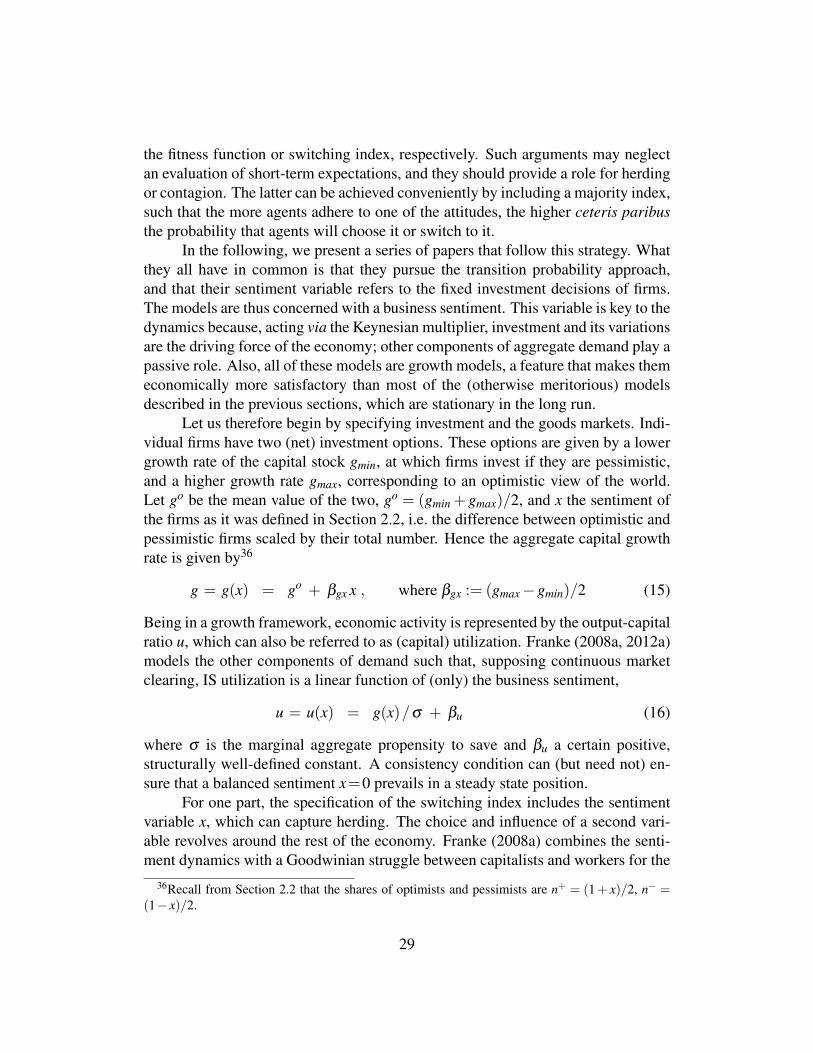
We fix φy = 1.80, ηx = ηy = 1.00 and study the changes in the system’s globalbehaviour under variations of the remaining coefficient φx. A deeper analysis of theresulting bifurcation phenomena when the dynamics changes from one regime toanother is given in Franke (2014). Here it suffices to view four selected values ofφx and the corresponding phase diagrams in the (x,y)-plane.

x=0

y=0

Figure 1: Phase diagrams of (8) for four different regimes.

12

Since tanh has a positive derivative everywhere, positive values of φx repre-sent a positive, i.e. destabilizing feedback in the sentiment adjustments. By contrast,φy > 0 together with ηx > 0 establishes a negative feedback loop for the sentimentvariable: an increase in x raises y and the resulting decrease in the switching indexlowers (the change in) x. The stabilizing effect will be dominant if φx is sufficientlysmall relative to φy. This is the case for φx = 0.90, which is shown in the top-leftdiagram of Figure 1. The two thin solid (black) lines depict the isoclines of thetwo variables; the straight line is the locus of y = 0 and the curved line is x = 0.Their point of intersection at (xo,yo) = (0,0) is the equilibrium point of system (8).Convergence towards it takes place in a cyclical manner.

The equilibrium (xo,yo) and the y = 0 isocline are, of course, not affected bythe changes in φx. On the other hand, increasing values of this parameter shift theisocline x = 0 downward to the left of the equilibrium and upward to the right of it.The counterclockwise motions are maintained, but at our second value φx = 2.20,they locally spiral outward, that is, the equilibrium has become unstable. Never-theless, further away from the equilibrium the centripetal forces prove dominantand generate spirals pointing inward. As a consequence, there must be one orbitin between that neither spirals inward nor outward. Such a closed orbit is indeedunique and constitutes a limit cycle that globally attracts all trajectories, whereverthey start from (except the equilibrium point itself). This situation is shown in thetop-right panel of Figure 1.

If φx increases sufficiently, the shifts of the x = 0 isocline are so pronouncedthat it cuts the straight line at two (but only two) additional points (x1,y1) and(x2,y2). One lies in the lower-left corner and the other symmetrically in the upper-right corner of the phase diagram. First, over a small range of φx, these outer equi-libria are unstable, after that, for all φx above a certain threshold, they are alwayslocally stable. The latter case is illustrated in the bottom-left panel of Figure 1,where the parameter has increased to φx = 2.96 (the isoclines are not shown here,so as not to overload the diagram).

The two shaded areas are the basins of attraction of (x1,y1) and (x2,y2), eachsurrounded by a repelling limit cycle. Remarkably, the stable limit cycle from φx =2.20 has survived these changes; it has become wider, encompasses the two outerequilibria together with their basins of attraction, and attracts all motions that donot start there.

The extreme equilibria move toward the limits of the domain of the sentimentvariable, x =±1, as φx increases. They do this faster than the big limit cycle widens.Eventually, therefore, the outer boundaries of the basins of attraction touch the bigcycle, so to speak. This is the moment when this orbit disappears, and with it allcyclical motions. The bottom-right panel of Figure 1 for φx = 3.00 demonstratesthat then the trajectories either converge to the saddle point (xo,yo) in the middle,

13

if they happen to start on its stable arm, or they converge to one of the other twoequilibria.

To sum up, whether the obvious, the ‘natural’ equilibrium (xo,yo) is stableor unstable, system (8) shows a broad scope for cyclical trajectories. Furthermore,whether there are additional outer equilibria or not, there is also broad scope forself-sustaining cyclical behaviour, that is, oscillations that do not explode and, evenin the absence of exogenous shocks, do not die out, either.

3 An early generation of models

Already soon after the publication of Weidlich and Haag’s book (1983) in whichtheir transition probability approach was advanced, attempts were made to utilizethis concept for macroeconomic modelling. Examples that we know of are Kraftet al. (1986), Haag et al. (1987), Weise and Kraft (1988), and Weidlich and Braun(1992). However, these contributions received vurtually no attention in the researchcommunity. Apart from the dominance of mainstream economics and the papers’reference to the unfamiliar apparatus of statistical mechanics, two further reasonsseem to be responsible for this neglect. The economic topics addressed by theseauthors were somewhat detached, or ‘exotic‘, and ordinary readers soon becameoverwhelmed by a lot of specification details, so that they could no longer appreci-ate the essence of the basic approach and its potential.

Let us therefore begin our survey with Kirman’s (1993) seminal paper abouta biological phenomenon published in an economic journal. The story he tells cannevertheless be immediately understood by any non-specialist. It is about a popu-lation of ants that can live on two permanently identical food sources, the questionbeing how the ants are distributed between the two in the long run. While intuitivelyit may seem that they would be split evenly, in experiments the ants were typicallyobserved to stabilize in a very unbalanced situation: a sizeable majority exploits onesource and the rest the other, but eventually, once in a while, reswitching betweenthe two sources occurs.

These repeated finding suggest that one should look for a simple model toexplain this majority building. Kirman’s paper is a fascinating and convincing pro-posal in this direction. He slices time into short periods, where in each period twoants meet at random. In such an encounter, the first ant is converted to the sec-ond ant’s food source with a given probability; with another (small) probability, itchanges sources independently. Kirman is able to compute the long-run distribu-tion between the two sources and thus prove that, over a certain range of parametervalues, the experimentally observed behaviour does indeed evolve. At the heart of

14

the result is the mechanism of herding (contagion, mimicking, recruitment are syn-onymous expressions). This means that the more ants feed on the first source, thehigher the probability of an ant from the other type being converted; and the lowerthe probability of a reverse change.

The constituent part of Kirman’s approach is the concept of transition prob-abilities. In fact, his model is quite similar in kind to the transition probabilityapproach presented in Section 2.2 before one considers the limit of an infinite pop-ulation, N → ∞, when the switching index s is an increasing function of the ma-jority index x (which was referred to there as the agents’ sentiment). The onlyessential difference is that, with Kirman’s specification, contrary to what happensin our equation (5), the intrinsic noise resulting from the ants’/agents’ individualrandom choices does not disappear as N becomes large (which may or may not bean attractive feature for model building).

Having understood Kirman’s model and its functioning, it is not a very far-fetched idea to incorporate its herding mechanism into a simple economic frame-work, expecting the salient properties to carry over and give rise to persistent cycli-cal behaviour. As far as we know, the first example of such a strategy is Westerhoffand Hohnisch (2007).19 They consider a population of N = 100 agents within thesetting of the Keynesian textbook multiplier. Fixing investment, they distinguishbetween optimistic and pessimistic agents who, respectively, have a higher andlower marginal propensity to consume. Hence output increases linearly with thenumber of optimistic consumers. In the random meetings, a pessimist is convertedto optimism with a probability that is higher when output has increased recentlythan when it has decreased, and vice versa for an optimist becoming a pessimist.

With suitable parameter values, this is in fact all that is needed to gener-ate the desired persistent cyclical fluctuations. To see this, consider the phase ofan expansion. Then the probability of switching from pessimism to optimism ishigher than the opposite change, which reinforces the upswing. This process will,however, slow down as the number of remaining pessimists and potential convertsdeclines. On the other hand, consumers can also change their attitude indepen-dently. Even though this may occur with a small probability only, this effect willeventually dominate the herding toward optimism (at the latest, when the entirepopulation has turned optimistic). Via the multiplier, the resulting decrease in thenumber of optimists reduces output, which in turn increases the overall probabilityof switching from optimism to pessimism. In this way, a turnaround is obtained and

19Before, Kirman’s model was successfully utilized to model speculation processes on financialmarkets (Kirman, 1991). Having outlined the close relationship of Kirman’s model to the transi-tion probability approach in Section 2.2, it would have also been possible in principle to try hisspecification for macroeconomic modelling.

15

the economy begins to enter a contraction.20

Westerhoff and Hohnisch (2010) introduce fiscal policy rules into this model.They point out that a fiscal stimulus does not only have a direct effect on economicactivity via the Keynesian multiplier, but that the increase in national income alsoaffects the agents’ sentiment and thus reinforces the initial effect. Hohnisch andWesterhoff (2008) triplicate Westerhoff’s first model, so to speak, by postulating thesame economy for three different countries. The national cycles are then seen to besynchronized if agents’ transition probabilities depend on economic performance athome and in the foreign countries.

In another series of papers, Westerhoff (2006a, 2006b, 2008) and Lines andWesterhoff (2006) introduce heterogeneous expectations into Samuelson’s (1939)multiplier-accelerator model.21 Instead of the usual dependence of investment onthe change in output most recently observed, in this case investment increases withthe expected change in that variable. A fraction of the agents adopt extrapolativeexpectations to predict output; the others rely on regressive expectations (that is,they expect output to gradually return to its equilibrium level). The other idea be-hind this approach is that the agents are aware of the fact that it is impossible tomaintain an upward or downward motion forever. For this reason, the more currentoutput deviates from its equilibrium, the less convincing the extrapolative expecta-tions appear to them. While nowadays one would perhaps apply the discrete choiceapproach to determine the population shares on the basis of this argument, thesepapers use another, straightforward functional specification.22

The fluctuations which are indeed obtained in this way are easy to explainonce it has been noted that the extrapolative expectations, when taken on their own,are destabilizing, whereas the regressive expectations are stabilizing. The formerdominate in a vicinity of the equilibrium, which drives the economy away from it.As the ‘misalignment’ increases, the agents become more prudent and the regressiveexpectations gain in weight. This puts a curb on the divergent tendencies and sooneror later reverses the path of the economy, causing it to return to more moderateoutput levels.

This mechanism is common to all the aforementioned papers; they merelydiffer with regard to a number of minor specification details. Furthermore, Wegeneret al. (2009) apply the idea of interacting extrapolative and regressive expectationsto Metzler’s (1941) model of an inventory cycle; unsurprisingly, as we know by

20Westerhoff (2010) considers a similar economy but, differing to our focus in this survey, placeshis agents on a square lattice, which allows him to study what emerges from their local interactions.

21In contrast to the models inspired by Kirman, these and all other models considered in the restof this section are purely deterministic.

22From our present point of view, this function might be called ad hoc, but it serves its purposeequally well.

16

now, it works out quite the same. In spite of being elementary, these results demon-strate that we have here a fairly straightforward device that may prove useful forgenerating persistent fluctuations, also in less pedagogical, more ambitious modelsettings.

Westerhoff (2006c) also studies extrapolative versus regressive expectations,but it seems the first macroeconomic paper that refers to Brock and Hommes (1997,1998) and employs the discrete choice approach to model the competition betweentwo rules or attitudes. Within the Keynesian textbook setting, Westerhoff concen-trates on consumption demand. He treats investment as being fixed and assumesthat consumption is proportional to expected output (that is, to national income).Instead of the previous misalignment argument to determine the shares of the twoforecast rules, they are judged by their relative success. Thus, the fitness whichenters the discrete choice probabilities is given by minus the most recent squaredprediction error. In addition, regressive expectations are supposed to be more costlythan their counterpart, which is expressed by subtracting a positive constant numberfrom their performance measure.

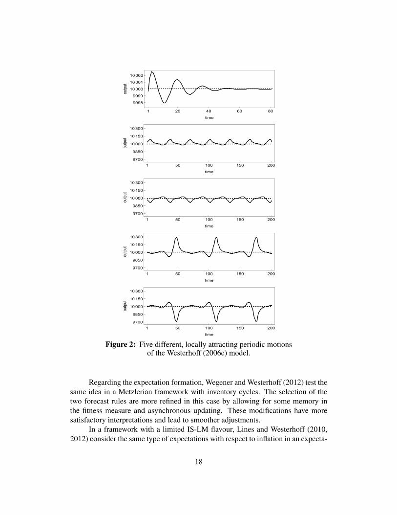
Westerhoff chooses a parametrization such that if all agents adopt extrap-olative expectations, divergence is not monotonic but occurs in a cyclical manner.While prediction errors are similar near the equilibrium, around the turning points,before and after them, it is the regressive expectations that are more successful,even after accounting for their cost. Their existence clearly depresses the next turn-ing point to come, but it is not entirely obvious what exactly prevents an ever in-creasing amplitude; indeed, in the simulations, the fluctuations always happen tobe bounded. This difficulty is illustrated by the cyclical patterns of the time se-ries, which can be rather complex. In any case, they do not look like a regularsine wave. It is even more remarkable that, although the trajectories converge toa periodic or quasi-periodic limit cycle, such an attractor is not unique. Moreover,also the equilibrium point itself is a local attractor. The example of Figure 2 showsthat, apart from the latter, the economy may converge to no less than four differentnon-degenerate periodic motions, depending on the initial conditions out of equi-librium.23

In this economic environment, Westerhoff (2006c) subsequently studies thescope for a stabilizing fiscal policy. The nonlinear, possibly complicated dynamicsprovides a serious challenge to government. Common ideas such as trend-offsettingor level-adjusting interventions turn out to be a mixed blessing. If the policy-makerschoose the wrong intensity—and here even tiny differences may matter—it canhappen that output fluctuations are amplified rather than dampened.

23In other simulations, Westerhoff obtains periodic orbits with larger variations in the amplitudefrom one (intermediate) cycle to another.

17

1 20 40 60 80

10000

10001

10002

9999

9998

time

output

1 50 100 150 200

10000

10150

10300

9700

9850

time

output

1 50 100 150 200

10000

10150

10300

9700

9850

time

output

1 50 100 150 200

10000

10150

10300

9700

9850

time

output

1 50 100 150 200

10000

10150

10300

9700

9850

time

output

Figure 2: Five different, locally attracting periodic motionsof the Westerhoff (2006c) model.

Regarding the expectation formation, Wegener and Westerhoff (2012) test thesame idea in a Metzlerian framework with inventory cycles. The selection of thetwo forecast rules are more refined in this case by allowing for some memory inthe fitness measure and asynchronous updating. These modifications have moresatisfactory interpretations and lead to smoother adjustments.

In a framework with a limited IS-LM flavour, Lines and Westerhoff (2010,2012) consider the same type of expectations with respect to inflation in an expecta-

18

tion-augmented price Phillips curve (keeping the rest as simple as possible).24 Onceagain, multiple locally attracting limit cycles are possible. In addition, it turns outthat wider regions of the parameter space yield a chaotic dynamic behaviour inthe sense of a strange attractor (its existence can be rigorously proven by comput-ing a certain mathematical indicator). The authors are also concerned with policyissues—monetary policy in this case. That is, in a Taylor-like manner, the centralbank may raise or lower the growth rate of the quantity of money in response tocurrent inflation and output growth. In particular, sufficiently strong reactions tothe latter are seen to provide potential for stabilization.

4 Heterogeneity and animal spirits in the New-Keynesianframework

4.1 De Grauwe’s modelling approach

Given that the New-Keynesian theory is the ruling paradigm in macroeconomics,Paul De Grauwe had a simple but ingenious idea to challenge it: accept the threebasic log-linearized equations for output, inflation and the interest rate of that ap-proach, but discard its underlying representative agents and rational expectations.This means that, instead, he introduces different groups of agents with heteroge-neous forms of bounded rationality, as it is called.25 Expectations have to be formedfor the output gap (the percentage deviations of output from its equilibrium trendlevel) and for the rate of inflation in the next period. For each variable, agents canchoose between two rules of thumbs where, as specified by the discrete choice ap-proach, switching between them occurs according to their forecasting performance.De Grauwe speaks of ‘animal spirits’ insofar as such a model is able to generate

24Lines and Westerhoff (2010) assume costly rational expectations rather than regressive expecta-tions. The dynamic properties are nevertheless fairly similar. On this occasion, we may also mentionan interesting alternative selection mechanism that was put forward in (almost) the same model byDa Silveira and Lima (2014), which they call satisficing evolutionary dynamics. It states that anindividual agent will only choose the more efficient rule if the performance differential exceeds acertain threshold, where these thresholds are randomly distributed across the population of agents.The authors prove that this leads to a locally stable equilibrium, a result that, however, may also bedue in part to the fact that the extrapolative expectations are replaced with adaptive expectations.Furthermore, there was no exploration of the global dynamics.

25To be fair, Brazier et al. (2008) pursued a similar idea in an overlapping-generations model withmoney growth and expectations about inflation. This paper proved, however, to be less influentialthan De Grauwe’s work.

19

waves of optimistic and pessimistic forecasts, notions that are excluded from theNew-Keynesian world by construction.26

The following three-equation model is taken from De Grauwe (2008a), whichis the first in a series of similar versions that have subsequently been studied in DeGrauwe (2010, 2011, 2012a,b). The term ‘three-equation’ refers to the three lawsthat determine the output gap y, the rate of inflation π , and the nominal rate ofinterest i set by the central bank. The symbols π? and i? denote the central bank’starget rates of inflation and interest, which are known and taken into account by theagents in the private sector. All parameters are positive where, more specifically, ay,by are weighting coefficients between 0 and 1. Eagg

t are the aggregated expectationsof the heterogeneous agents using information up to the beginning of the presentperiod t. They are substituted for the mathematical expectation operator Et , theaforementioned rational expectations. Then, the three equations are:

yt = ay Eaggt yt+1 + (1−ay)yt−1 + ai [it −Eagg

t πt+1 − (i?−π?)] + εy,t (9)

πt = bπ Eaggt πt+1 + (1−bπ)πt−1 + by yt + επ,t (10)

it = ci it−1 + (1−ci) i? + cπ (πt −π?) + cy yt + εi,t (11)

Equation (9) for the output gap is usually referred to as an IS equation, here inhybrid form, which means that the expectation term is combined with a one-periodlag of the same variable. The Phillips curve in (10), likewise in hybrid form, isviewed as representing the supply side of the economy. Equation (11) is a Taylorrule with interest rate smoothing, that is, it contains the lagged interest rate on theright-hand side.27 The terms εy,t , επ,t , εi,t are white noise disturbances, interpretedas demand, supply and monetary policy shocks, respectively. Qualitatively littlewould change if some serial correlation were allowed for them.

The aggregate expectations in these equations are convex combinations oftwo (extremely) simple forecasting rules. With respect to the output gap, De Grauweconsiders optimistic and pessimist forecasters, predicting a fixed positive and neg-ative value of y, respectively. With respect to the inflation rate, he distinguishesbetween agents who believe in the central bank’s target and so-called extrapolators,who predict that next period’s inflation will be last period’s inflation.28 Accord-

26It has already been indicated in footnote 1 that the special branch of ‘sunspot equilibria’ withinthe DSGE literature makes reference to ‘animal spirits’, too, but that these concepts are fundamen-tally different from the mechanisms in the present models. As the term ‘sunspots’ suggests, thewaves generated there have an exogenous source, while De Grauwe emphasizes their endogenousorigin in his approach.

27De Grauwe mostly simplifies his equations by putting i? = π? = 0.28It would be more appropriate to call the latter naive expectations; cf. De Grauwe and Mac-

chiarelli (2015, p. 97).

20

ingly, with g > 0 as a positive constant, nopt as the share of optimistic agents re-garding output, and ntar as the share of central bank believers regarding inflation,expectations are given by

Eoptt yt+1 = g , E pess

t yt+1 = −g

Etart πt+1 , = π? Eext

t πt+1 = πt−1

Eaggt yt+1 = nopt

t Eoptt yt+1 + (1−nopt

t )E pesst yt+1

Eaggt πt+1 = ntar

t Etart πt+1 + (1−ntar

t )Eextt πt+1

(12)

In other papers, De Grauwe alternatively stipulates so-called fundamental and ex-trapolative output forecasters, E f un

t yt+1 = 0 and Eextt yt+1 = yt−1. However, the

dynamic properties of his model are not essentially affected by such a respecifica-tion.

The populations shares of the heterogeneous agents are determined by thesuitably adjusted discrete choice equations (1), (2). Denoting the measures of fit-ness that apply here by Uopt , U pess, U tar, Uext , we have

noptt =

exp(βUoptt−1)

exp(βUoptt−1) + exp(βU pess

t−1 )

ntart =

exp(βU tart−1)

exp(βU tart−1) + exp(βUext

t−1)

(13)

Conforming to the principle that better forecasts attract a higher share of agents,fitness is defined by the negative (infinite) sum of the past squared prediction errors,where the past is discounted with geometrically declining weights. Hence, with aso-called memory coefficient 0 < ρ < 1, superscripts A = opt, pess, tar, ext andvariables z = y,π in obvious assignment,

UAt = −

∞

∑k=1

ωk (zt−k − EAt−k−1 zt−k)2 , ωk = (1−ρ)ρ

k

= −ρ {(1−ρ)(zt−1 − EAt−2 zt−1)2 + UA

t−1 }(14)

This specification of the weights ωk makes sure that they add up to unity. Thesecond expression in (14) is an elementary mathematical reformulation. It allows arecursive determination of the fitness, which is more convenient and more preciselycomputable than an approximation of an infinite series.

Equation (14) completes the model. De Grauwe makes no explicit referenceto an equilibrium of the economy (or possibly several of them?) and does not

21

attempt to characterize its stability or instability. He proceeds directly to numericalsimulations and then discusses what economic sense can be made of what we see.Depending on the specific focus in his papers, additional computer experimentswith some modifications may follow.

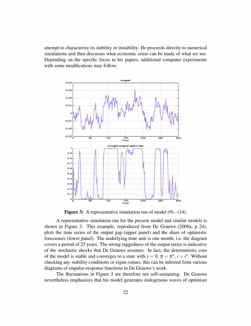
Figure 3: A representative simulation run of model (9) – (14).

A representative simulation run for the present model and similar models isshown in Figure 3. This example, reproduced from De Grauwe (2008a, p. 24),plots the time series of the output gap (upper panel) and the share of optimisticforecasters (lower panel). The underlying time unit is one month, i.e. the diagramcovers a period of 25 years. The strong raggedness of the output series is indicativeof the stochastic shocks that De Grauwe assumes. In fact, the deterministic coreof the model is stable and converges to a state with y = 0, π = π?, i = i?. Withoutchecking any stability conditions or eigen-values, this can be inferred from variousdiagrams of impulse-response functions in De Grauwe’s work.

The fluctuations in Figure 3 are therefore not self-sustaining. De Grauwenevertheless emphasizes that his model generates endogenous waves of optimism

22

and pessimism. This characterization may be clarified by a longer quote from DeGrauwe (2010, p. 12):

“These endogenously generated cycles in output are made possible by a self-fulfilling mechanism that can be described as follows. A series of randomshocks creates the possibility that one of the two forecasting rules, say the ex-trapolating one, delivers a higher payoff, i.e. a lower mean squared forecast er-ror (MSFE). This attracts agents that were using the fundamentalist rule. If thesuccessful extrapolation happens to be a positive extrapolation, more agentswill start extrapolating the positive output gap. The ‘contagion-effect’ leadsto an increasing use of the optimistic extrapolation of the output-gap, whichin turn stimulates aggregate demand. Optimism is therefore self-fulfilling. Aboom is created. At some point, negative stochastic shocks and/or the reactionof the central bank through the Taylor rule make a dent in the MSFE of theoptimistic forecasts. Fundamentalist forecasts may become attractive again,but it is equally possible that pessimistic extrapolation becomes attractive andtherefore fashionable again. The economy turns around.

These waves of optimism and pessimism can be understood to be searching(learning) mechanisms of agents who do not fully understand the underlyingmodel but are continuously searching for the truth. An essential characteristicof this searching mechanism is that it leads to systematic correlation in beliefs(e.g. optimistic extrapolations or pessimistic extrapolations). This systematiccorrelation is at the core of the booms and busts created in the model.”

Thus, in certain stages of a longer cycle, the optimistic expectations are superior,which increases the share of optimistic agents and enables output to rise, whichin turn reinforces the optimistic attitude. This mechanism is evidenced by the co-movements of yt and nopt

t in Figure 3 and conforms to the positive feedback loophighlighted in a comment on the small and stylized system (8) above.29 A sta-bilizing counter-effect is not as clearly recognizable. De Grauwe only alludes tothe central bank’s reactions in the Taylor rule, when positive output gaps and infla-tion rates above their target (which will more or less move together) lead to bothhigher nominal and real interest rates. This is a channel that puts a curb on yt in theIS equation. In addition, a suitable sequence of random shocks may occasionallywork in the same direction and initiate a turnaround.

The New-Keynesian theory is proud of its “microfoundations”. Within theframework of the representative agents and rational expectations, they derive themacroeconomic IS equation (9) and the Phillips curve (10) as log-linear approxi-mations to the optimal decision rules of intertemporal optimization problems. As

29De Grauwe (2010, p. 14) reports that the correlation between the fraction of optimists and theoutput gap is as high as 0.86. This requires the intensity of choice β to be sufficiently high and thememory coefficient ρ to be less than one (though only slightly so); see ibid., pp. 14f.

23

these two assumptions have now been dropped, the question arises of the theoreticaljustification of (9) and (10). Two answers can be given.

First, Branch and McGough (2009) are able to derive these equations invok-ing two groups of individually boundedly rational agents, provided that their ex-pectation formation satisfies a set of seven axioms.30 The authors point out thatthe axioms are not only necessary for the aggregation result, but some of themcould also be considered rather restrictive; see, especially, Branch and McGough(2009, p. 1043). Furthermore, it may not appear very convincing that the agentsare fairly limited in their forecasts, and yet they endeavour to maximize their ob-jective function over an infinite time horizon and are smart enough to compute thecorresponding first-order Euler conditions.

Acknowledging these problems, the second answer is that the equations makegood economic sense even without a firm theoretical basis. Thus, one is willingto pay a price for the convenient tractability obtained, arguing that more consis-tent attempts might be undertaken in the future. In fact, De Grauwe’s approachalso succeeded in gaining the attention of New-Keynesian theorists and a certainappreciation by the more open-minded proponents. This is indeed one of the rareoccasions where orthodox and heterodox economists are able and willing to discussissues by starting out from a common basis.

Branch and McGough (2010) consider a similar version to eqs (9) – (11)where, besides naive expectations, they still admit rational expectations. However,the latter are more costly, meaning that they may be outperformed by boundedlyrational agents in tranquil times, in spite of their systematic forecast errors. Forgreater clarity, the economy is studied in a deterministic setting (hence rational ex-pectations amount to perfect foresight). The authors are interested in the stationarypoints of this dynamics: in general there are multiple equilibria and the questions iswhich are stable/unstable, and what are the population shares prevailing in them.

Branch and McGough’s analysis provides a serious challenge for the rationalexpectations hypothesis. Its recommendation to monetary policy is to guaranteedeterminacy in models of this type (this essentially amounts to the Taylor principle,according to which the interest rate has to rise more than one-for-one with infla-tion). Branch and McGough illustrate that, in their framework, the central bankmay unwittingly destabilize the economy by generating complex (’chaotic’) dy-namics with inefficiently high inflation and output volatility, even if all agents areinitially rational. The authors emphasize that these outcomes are not limited to un-usual calibrations or a priori poor policy choices; the basic reason is rather the dual

30To be exact, the equations they obtain do not contain the lagged endogenous variable on theright-hand side. A model in a similar spirit but with more specific assumptions is studied by Massaro(2013).

24

attracting and repelling nature of the steady state values of output and inflation.Anufriev et al. (2013) abstract from output and limit themselves to a version

of (10) with only expected inflation on the right-hand side. Since there is no interestrate smoothing in their Taylor rule (c1 = 0) and, of course, no output gap either, theinflation rate is the only dynamic variable. These simplifications allow the authorsto consider greater variety in the formation of expectations and to study their effectsalmost in a vacuum. In this case, too, the main question is whether, in the absence ofrandom shocks, the system will converge to the rational expectations equilibrium.This is possible but not guaranteed because, again, certain ecologies of forecastingrules can lead to multiple equilibria, where some are stable and give rise to intrinsicheterogeneity.

Maintaining the (stochastic) equations (9), (10) (but without the lagged vari-ables on the right-hand side) and considering different dating assumptions in theTaylor rule (likewise without interest rate smoothing), Branch and Evans (2011)obtain similar results, broadly speaking. They place particular interest in a possibleregime-switching of the output and inflation variances (an important empirical issuefor the US economy), and in the implications of heterogeneity for optimal monetarypolicy.

Drager (2016) examines the interplay between fully rational (but costly) andboundedly rational (but costless) expectations in a subvariant of the New-Keynesianapproach, which is characterized by a so-called rational inattentiveness of agents.As a result of this concept, entering the model equations for quarter t are not onlycontemporary but also past expectations about the variables in quarter t+1. The au-thor’s main concern is with the model’s ability to match certain summary statisticsand, in particular, the empirically observed persistence in the data. Not the least dueto the flexible degree of inattention, which is brought about by the agents’ switchingbetween full and bounded rationality (in contrast to the case where all agents arefully rational, when the degree is fixed), the model turns out to be superior to themore orthodox model variants.31

4.2 Modifications and extensions

The attractiveness of De Grauwe’s modelling strategy is also shown by a numberof papers that take his three-equation model as a point of departure and combine itwith a financial sector. To be specific, this means that a financial variable is added toeq. (9), (10) or (11), and that the real economy also feeds back on financial markets

31The two precursory working papers Drager (2010, 2011) may help generate a better understand-ing of the more elaborate parts of this analysis and of the conditions that may give rise to the superiorresults with the flexible-degree version.

25

via the output gap or the inflation rate. It is here a typical conjecture, which thenneeds to be tested, that a financial sector tends to destabilize the original model insome sense; for example, output or inflation may become more volatile.

An early extension of this kind is the integration of a stock market in DeGrauwe (2008b). He assumes that an increase in stock prices has a positive influ-ence on output in the IS equation and a negative influence on inflation in the Phillipscurve (the latter because this reduces marginal costs). In addition, it is of specialinterest that the central bank can try to lean against the wind by including a positiveeffect of stock market booms in its interest rate reaction function. The stock pricesare determined, in turn, by expected dividends discounted by the central bank’s in-terest rate plus a constant markup. The actual dividends are a constant fraction ofnominal GDP, i.e. their forecasts are closely linked to the agents’ forecasts of outputand inflation.

In a later paper, De Grauwe and Macchiarelli (2015) include a banking sectorin the baseline model. In this case, the negative spread between the loan rate andthe central bank’s short-term interest rate enters the IS equation in order to capturethe cost of bank loans. Along the lines of the financial accelerator by Bernankeet al. (1999), banks are assumed to reduce this spread as firms’ equity increaseswhich, by hypothesis, moves in step with their loan demand. Besides yt , πt , it , themodel contains private savings and the borrowing-lending spread as two additionaldynamic variables. In the final sections of the paper, the model is extended byintroducing variable share prices and determining them analogously to De Grauwe(2008b).

De Grauwe and Gerba (2015a) is a very comprehensive contribution thatstarts out from De Grauwe and Macchiarelli (2015), but specifies a richer structureof the financial sector, which also finds its way into the IS equation. One conse-quence of the extension is that capital now shows up as another dynamic variable,and that new types of shocks are considered.32 Once again, the discrete choice ver-sion is contrasted to the world with rational expectations. In a follow-up paper, DeGrauwe and Gerba (2015b) introduce a bank-based corporate financing friction andevaluate the relative contribution of that friction to the effectiveness of monetarypolicy. On the whole, it is impressive work, but, given the long list of numericalparameters to set, readers have to place their trust in it.

Lengnick and Wohltmann (2013) and, in a more elaborated version, (2016)choose a different approach to add a stock market to the baseline model.33 There are

32There are lots of microfoundation details in the first section. Unexperienced readers shouldnot be deterred by this, but may proceed to Section 3.5, which provides a familiar, though morecolourful picture.

33In eqs (9) and (10) they consider three types of expectations: targeting, naive and extrapolativeexpectations proper.

26

two channels through which stock prices affect the real side of the economy. One isa negative influence in the Phillips curve, which is interpreted as an effect on mar-ginal cost, the other is the difference between stock price and goods price inflationin the IS equation, which may increase output. The modelling of the stock market,on the other hand, is borrowed from the burgeoning literature on agent-based spec-ulative demands for a risky asset. Such a market is populated by fundamentalisttraders and trend chasers who switch between these strategies analogously to (13)and (14). The market is now additionally influenced by the real sector through theassumption that the fundamental value of the shares is proportional to the outputgap. Furthermore, besides speculators, there is a stock demand by optimizing pri-vate households, which increases with output and decreases with the interest rateand higher real stock prices.

While in the simulations the authors maintain the usual quarter as the lengthof the adjustment period in (9) – (11) for the real sector, they specify financial trans-actions on a daily basis and use time aggregates for their feedback on the quarterlyequations. Even in isolation and without random shocks, the stock market dynamicsis known for its potential to generate endogenous booms and busts. The spill-overeffects can now cause a higher volatility in the real sector. For example, it can mod-ify the original effects of a given shock in the impulse-response functions and makethem hard to predict.34 One particular concern of the two papers is a possible stabi-lization through monetary policy, another is a taxation of the financial transactionsor profits. An important issue is whether a policy that is effective under rationalexpectations can also be expected to be so in an environment with heterogeneousand boundedly rational agents.

Scheffknecht and Geiger’s (2011) modelling is in a similar spirit (includingthe different time scales for the real and financial sector), but limits itself to onechannel from the stock market to the three-equation baseline specification. To thisend, the authors add a risk premium ζt (i.e. the spread between a credit rate and it)to the short-term real interest rate in (9). The transmission is a positive impact ofthe change in stock prices on ζt , besides effects from yt , it and the volatilities (i.e.variances) of yt ,πt , it on this variable.

A new element is an explicit consideration of momentum traders’ balancesheets (but only of theirs, for simplicity). They are made up of the value of theshares they hold and money, which features as cash if it is positive and debt if itis negative. This brings the leverage ratios of these traders into play, which may

34The reference for the authors’ impulse-response functions (IRFs) is not an equilibrium position,but an entire stochastic simulation run. Subsequently, the model is run a second time with the samerandom shocks, except for one shock in the initial period. The IRFs are then the difference in thevariables from these two runs.

27

constrain them in their asset demands. Although the latter extension is not free ofinconsistencies, these are ideas worth considering.35

5 Herding and objective determinants of investment

Apart from the models inspired by Kirman (1993), the models discussed so farwere concerned with expectations about an economic variable in the next period.Here, a phenomenon to which an expression like ‘animal spirits’ may apply occurswhen the agents rush toward one of the two forecast rules. However, this behaviouris based on objective factors, normally publicly available statistics. Most promi-nently, they contrast expected with realized values and then evaluate the forecastperformance of the rules.

In the present section, we emphasize that the success of decisions involvinga longer time horizon, in particular, cannot be judged from such a good or bad pre-diction, or from corresponding profits in the next quarter. It takes several years toknow whether an investment in fixed capital, for example, was worth undertaking.Furthermore, decisions of that kind must, realistically, take more than one dimen-sion into account. As a consequence, expectations are multi-faceted and far morediffuse in nature. In these situations, the third paragraph of the Keynes quotation inthe introductory section becomes relevant, where he points out that “we endeavor toconform with the behavior of the majority or the average”, which “leads to what wemay strictly term a conventional judgment.” In other words, central elements areconcepts such as a (business or consumer) sentiment or climate, or a general stateof confidence. In the language of tough business men, it is not only their skills, butalso their gut feelings that make them so successful.

Therefore, as an alternative to the usual focus on next-period expectations ofa specific macroeconomic variable, we may formulate the following axiom: long-term decisions of the agents are based on sentiment, where, as indicated by Keynes,with agents’ orientation toward the behaviour of the majority, this expression mayalso connote herding. In terms of ‘animal spirits’, we propose that in the mod-els under consideration so far we have animal spirits in a weak sense, whereas inthe context outlined above we have animal spirits in a strong sense; animal spiritsproper, so to speak.

The discrete choice and transition probability approaches can also be used tomodel animal spirits in the strong sense. Crucial for this is specifying argumentswith which the probabilities are supposed to vary, that is, specifying what was called

35Two aspects are: (1) There is nobody in the model from which momentum traders could borrow,and whose balance sheet would be affected, too. (2) Neither the direct nor the indirect cost ofborrowing shows up in the fitness function of momentum traders.

28

the fitness function or switching index, respectively. Such arguments may neglectan evaluation of short-term expectations, and they should provide a role for herdingor contagion. The latter can be achieved conveniently by including a majority index,such that the more agents adhere to one of the attitudes, the higher ceteris paribusthe probability that agents will choose it or switch to it.

In the following, we present a series of papers that follow this strategy. Whatthey all have in common is that they pursue the transition probability approach,and that their sentiment variable refers to the fixed investment decisions of firms.The models are thus concerned with a business sentiment. This variable is key to thedynamics because, acting via the Keynesian multiplier, investment and its variationsare the driving force of the economy; other components of aggregate demand play apassive role. Also, all of these models are growth models, a feature that makes themeconomically more satisfactory than most of the (otherwise meritorious) modelsdescribed in the previous sections, which are stationary in the long run.

Let us therefore begin by specifying investment and the goods markets. Indi-vidual firms have two (net) investment options. These options are given by a lowergrowth rate of the capital stock gmin, at which firms invest if they are pessimistic,and a higher growth rate gmax, corresponding to an optimistic view of the world.Let go be the mean value of the two, go = (gmin + gmax)/2, and x the sentiment ofthe firms as it was defined in Section 2.2, i.e. the difference between optimistic andpessimistic firms scaled by their total number. Hence the aggregate capital growthrate is given by36

g = g(x) = go + βgx x , where βgx := (gmax−gmin)/2 (15)

Being in a growth framework, economic activity is represented by the output-capitalratio u, which can also be referred to as (capital) utilization. Franke (2008a, 2012a)models the other components of demand such that, supposing continuous marketclearing, IS utilization is a linear function of (only) the business sentiment,

u = u(x) = g(x)/σ + βu (16)

where σ is the marginal aggregate propensity to save and βu a certain positive,structurally well-defined constant. A consistency condition can (but need not) en-sure that a balanced sentiment x=0 prevails in a steady state position.

For one part, the specification of the switching index includes the sentimentvariable x, which can capture herding. The choice and influence of a second vari-able revolves around the rest of the economy. Franke (2008a) combines the senti-ment dynamics with a Goodwinian struggle between capitalists and workers for the

36Recall from Section 2.2 that the shares of optimists and pessimists are n+ = (1 + x)/2, n− =(1− x)/2.

29

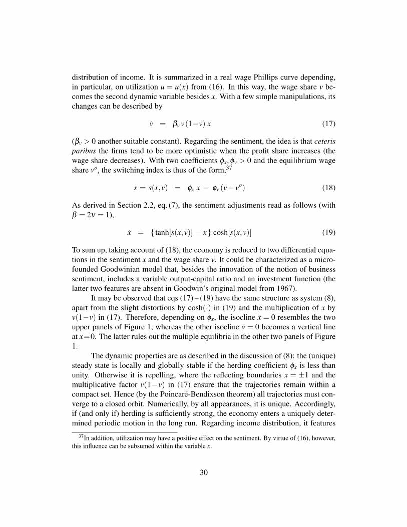
distribution of income. It is summarized in a real wage Phillips curve depending,in particular, on utilization u = u(x) from (16). In this way, the wage share v be-comes the second dynamic variable besides x. With a few simple manipulations, itschanges can be described by

v = βv v(1−v) x (17)

(βv > 0 another suitable constant). Regarding the sentiment, the idea is that ceterisparibus the firms tend to be more optimistic when the profit share increases (thewage share decreases). With two coefficients φx,φv > 0 and the equilibrium wageshare vo, the switching index is thus of the form,37

s = s(x,v) = φx x − φv (v− vo) (18)

As derived in Section 2.2, eq. (7), the sentiment adjustments read as follows (withβ = 2ν = 1),

x = { tanh[s(x,v)] − x} cosh[s(x,v)] (19)

To sum up, taking account of (18), the economy is reduced to two differential equa-tions in the sentiment x and the wage share v. It could be characterized as a micro-founded Goodwinian model that, besides the innovation of the notion of businesssentiment, includes a variable output-capital ratio and an investment function (thelatter two features are absent in Goodwin’s original model from 1967).

It may be observed that eqs (17) – (19) have the same structure as system (8),apart from the slight distortions by cosh(·) in (19) and the multiplication of x byv(1−v) in (17). Therefore, depending on φx, the isocline x = 0 resembles the twoupper panels of Figure 1, whereas the other isocline v = 0 becomes a vertical lineat x=0. The latter rules out the multiple equilibria in the other two panels of Figure1.

The dynamic properties are as described in the discussion of (8): the (unique)steady state is locally and globally stable if the herding coefficient φx is less thanunity. Otherwise it is repelling, where the reflecting boundaries x = ±1 and themultiplicative factor v(1−v) in (17) ensure that the trajectories remain within acompact set. Hence (by the Poincare-Bendixson theorem) all trajectories must con-verge to a closed orbit. Numerically, by all appearances, it is unique. Accordingly,if (and only if) herding is sufficiently strong, the economy enters a uniquely deter-mined periodic motion in the long run. Regarding income distribution, it features

37In addition, utilization may have a positive effect on the sentiment. By virtue of (16), however,this influence can be subsumed within the variable x.

30

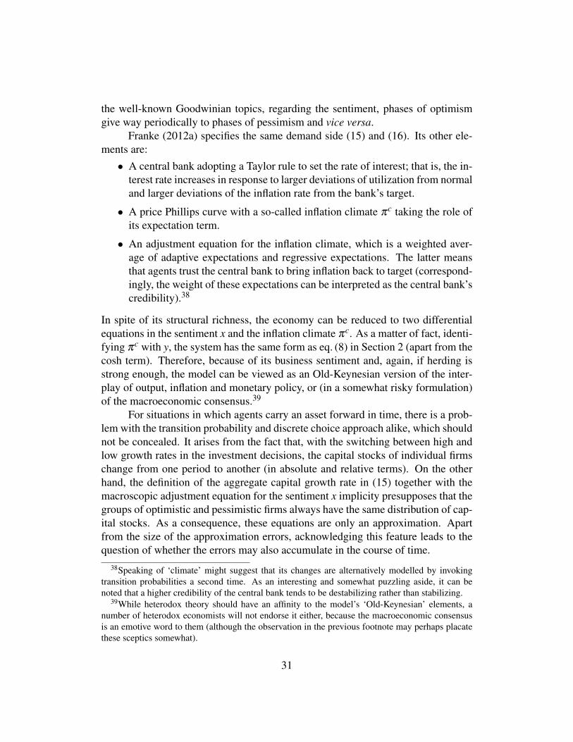
the well-known Goodwinian topics, regarding the sentiment, phases of optimismgive way periodically to phases of pessimism and vice versa.

Franke (2012a) specifies the same demand side (15) and (16). Its other ele-ments are:

• A central bank adopting a Taylor rule to set the rate of interest; that is, the in-terest rate increases in response to larger deviations of utilization from normaland larger deviations of the inflation rate from the bank’s target.

• A price Phillips curve with a so-called inflation climate πc taking the role ofits expectation term.

• An adjustment equation for the inflation climate, which is a weighted aver-age of adaptive expectations and regressive expectations. The latter meansthat agents trust the central bank to bring inflation back to target (correspond-ingly, the weight of these expectations can be interpreted as the central bank’scredibility).38

In spite of its structural richness, the economy can be reduced to two differentialequations in the sentiment x and the inflation climate πc. As a matter of fact, identi-fying πc with y, the system has the same form as eq. (8) in Section 2 (apart from thecosh term). Therefore, because of its business sentiment and, again, if herding isstrong enough, the model can be viewed as an Old-Keynesian version of the inter-play of output, inflation and monetary policy, or (in a somewhat risky formulation)of the macroeconomic consensus.39

For situations in which agents carry an asset forward in time, there is a prob-lem with the transition probability and discrete choice approach alike, which shouldnot be concealed. It arises from the fact that, with the switching between high andlow growth rates in the investment decisions, the capital stocks of individual firmschange from one period to another (in absolute and relative terms). On the otherhand, the definition of the aggregate capital growth rate in (15) together with themacroscopic adjustment equation for the sentiment x implicity presupposes that thegroups of optimistic and pessimistic firms always have the same distribution of cap-ital stocks. As a consequence, these equations are only an approximation. Apartfrom the size of the approximation errors, acknowledging this feature leads to thequestion of whether the errors may also accumulate in the course of time.

38Speaking of ‘climate’ might suggest that its changes are alternatively modelled by invokingtransition probabilities a second time. As an interesting and somewhat puzzling aside, it can benoted that a higher credibility of the central bank tends to be destabilizing rather than stabilizing.

39While heterodox theory should have an affinity to the model’s ‘Old-Keynesian’ elements, anumber of heterodox economists will not endorse it either, because the macroeconomic consensusis an emotive word to them (although the observation in the previous footnote may perhaps placatethese sceptics somewhat).

31

Yanovski (2014) goes back to the micro level of the transition probabilityapproach to inquire into this problem. Considering a finite population, he mod-els each firm and its probability calculus individually and also keeps track of thecapital stocks resulting from these decisions (modelling that requires a few addi-tional specifications to be made for the micro level). In short, the author finds thatthe approximation problem does not appear to be very serious. Of course, everymacro model that uses the transition probability or discrete choice approach mustbe reviewed separately, but this first result is encouraging.

Interestingly, Yanovski discovers another problem, which concerns the sizedistribution of capital stocks: it tends to be increasingly dispersed over time. Theresult that some firms become bigger and bigger may or may not be attractive.Yanovski subsequently tries several specification details that may entail a boundedwidth of the size distribution in the long run. To them it is crucial to relax theassumption of uniform transition probabilities, and that additional, firm-specificarguments are proposed to enter them. Within a parsimonious framework, thesediscussions can provide a better understanding of the relationships between microand macro.40

Going back to macrodynamics, Lojak (2015) adds a financial side to the mon-etary policy and output-inflation nexus in Franke (2012a). Besides the different sav-ing propensities for workers and rentiers households, which yield a more involvedIS equation for goods market clearing, it makes the firms’ financing of fixed invest-ment explicit. This work distinguishes between internal sources, i.e. the retainedearnings of the firms, and external sources, i.e. their borrowing from the rentiers(possibly with commercial banks as intermediates). In this way, a third dynamicvariable is introduced into the model, the firms’ debt-to-capital ratio. It feeds backon the real sector by a negative effect of higher indebtedness on the switching in-dex for the business sentiment x (which again demonstrates the flexibility of thisconcept).

Motivated by the discussion of Minskian themes in other macro models, theauthor concentrates on cyclical scenarios and here, in particular, on the comove-ments of the debt-asset ratio. While it is usually taken for granted that it lags capitalutilization, the author shows that this is by no means obvious. This finding is anexample of the need to carefully reconsid the dynamic features of a real-financialinteraction.

In a follow-up paper, Lojak (2016) fixes the inflation rate for simplicity anddrops the assumption of a constant markup on the central bank’s short-term interest

40The discussion can thus be more transparent than in the so-called bottom-up models with manyheterogeneous agents (far more than two), which are creative but less ‘canonical’ than the approachunder consideration here.

32

rate to determine the loan rate. Instead, the markup is now supposed to increasewith the debt-asset ratio, d. This straightforward extension gives rise to additionalstrong nonlinearities. Most amazingly, in the original cyclical scenario of the two-dimensional (x,d) dynamics a second equilibrium with lower utilization and higherindebtedness comes into being (but not three as in Figure 1). It is also characterizedby a locally stable limit cycle around it. The limit cycle around the ‘normal’ equi-librium is maintained, so that two co-existing cyclical regimes are obtained. Notall of the phenomena that one can here observe are as yet fully understood, whichshows that it is work in progress and a fruitful field for further investigations. Inparticular, future research may consider the lending of commercial banks in finerdetail, and animal spirits may then play a role in this sector as well.

6 Reality checks

Even if the discrete choice and transition probabilities are reckoned to be a concep-tually attractive approach for capturing a sentiment dynamics, these specificationswould gain in significance if it can be demonstrated that they are compatible withwhat is observed in reality, or inferred from it. A straightforward attempt to learnabout people’s decision-making are controlled experiments with human subjects inthe laboratory. Regarding empirical testing in the usual sense, there are two differ-ent ways to try, a direct and a more indirect way. The first method treats a sentimentadjustment equation such as (3) or (5) as a single-equation estimation, where thevariable xt in (5) or the population shares n+

t , n−t in (3) are proxied by an economicsurvey. In fact, several such surveys provide so-called sentiment or climate indices.The second method considers a model as a whole and seeks to estimate its para-meters in one effort. Here, however, x or n+,n− remain unobserved variables, thatis, only ‘normal’ macroeconomic variables such as output, inflation, etc. are in-cluded as empirical data. These three types of a reality check are considered in thefollowing subsections.

6.1 Evidence from the lab

Self-inspection is not necessarily the best method to find out how people arrive attheir decisions. A more systematic way that approaches people directly in this mat-ter are laboratory experiments. To begin with, they indeed provide ample evidencethat the subjects use similarly simple heuristics to those considered in the modelsthat we have presented; see Assenza et al. (2014a) for a comprehensive literaturesurvey. A more specific point is whether the distribution of different rules withina population and its changes over time could be explained by the discrete choice

33

or transition probability approach. Several experiments at CeNDEF (University ofAmsterdam) allow a positive answer with respect to the former. In the setting ofa New-Keynesian three-equation model, Assenza et al. (2014b) find four qualita-tively different macro patterns emerging out of a self-organizing process where oneof four forecasting rules tends to become dominant in the consecutive rounds ofan experiment. The authors demonstrate that this is quite in accordance with thediscrete choice principle.41

In another study by Anufriev et al. (2016), where the series to be forecastedare exogenously generated prior to the experiments and the subjects have to choosebetween a small numbers of alternatives given to them, a discrete choice model canin most cases be successfully fitted to the subjects’ predictions. In particular, theexperimenters can make inference about the intensity of choice, although differenttreatments yield different values. For all of these studies, however, it has to betaken into account that a full understanding of the results requires the reader to getinvolved in a lot of details.

6.2 Empirical single-equation estimations

With respect to inference from empirical data, let us first consider surveys collectinginformation about the expectations or sentiment of a certain group in the economy.As far as we know, the first empirical test of this kind is Branch (2004). He is con-cerned with the Michigan survey where private households are asked on a monthlybasis for their expectations about future inflation. For his analysis, the author equipsthe respondents with three virtual predictor rules: naive (i.e. static) expectations,adaptive expectations, and the relatively sophisticated expectations obtained from avector autoregression that besides inflation includes unemployment, money growthand an interest rate. The fitness of these rules derives from the squared forecasterrors and a specific cost term (which has to be re-interpreted after the estimations).

The model thus set up is estimated by maximum likelihood. The estimate ofthe intensity of choice is significantly positive, such that all three rule are relevant(even the naive expectations) and their fractions exhibit nonnegligible fluctuationsover time. It is also shown that this model is markedly superior to two alternativesthat assume the forecasts are normally distributed around their constant or time-varying mean values across the respondents.

Branch (2007) is a follow-up paper using the same data. Here the forecastrules entering the discrete choice model are more elaborate than in his earlier pa-per. They are actually based on explanations from a special branch of the New-

41Two similar experimental studies for a financial market environment are Anufriev and Hommes(2012a, b).

34

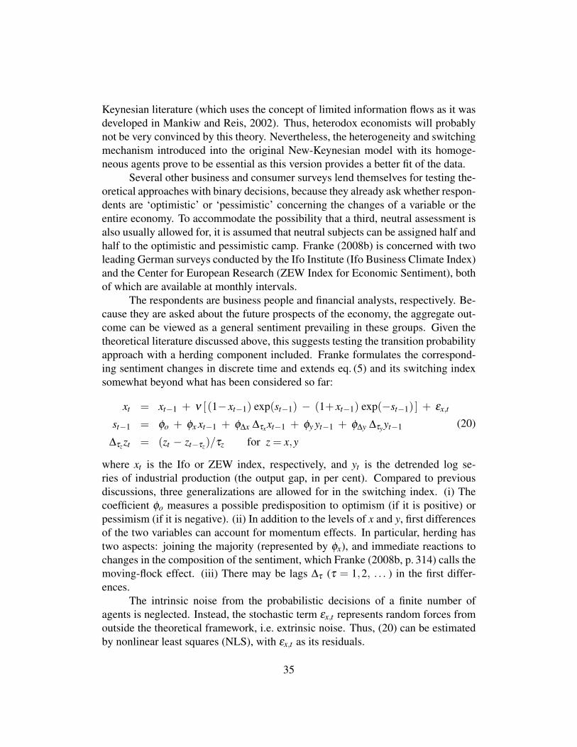
Keynesian literature (which uses the concept of limited information flows as it wasdeveloped in Mankiw and Reis, 2002). Thus, heterodox economists will probablynot be very convinced by this theory. Nevertheless, the heterogeneity and switchingmechanism introduced into the original New-Keynesian model with its homoge-neous agents prove to be essential as this version provides a better fit of the data.

Several other business and consumer surveys lend themselves for testing the-oretical approaches with binary decisions, because they already ask whether respon-dents are ‘optimistic’ or ‘pessimistic’ concerning the changes of a variable or theentire economy. To accommodate the possibility that a third, neutral assessment isalso usually allowed for, it is assumed that neutral subjects can be assigned half andhalf to the optimistic and pessimistic camp. Franke (2008b) is concerned with twoleading German surveys conducted by the Ifo Institute (Ifo Business Climate Index)and the Center for European Research (ZEW Index for Economic Sentiment), bothof which are available at monthly intervals.

The respondents are business people and financial analysts, respectively. Be-cause they are asked about the future prospects of the economy, the aggregate out-come can be viewed as a general sentiment prevailing in these groups. Given thetheoretical literature discussed above, this suggests testing the transition probabilityapproach with a herding component included. Franke formulates the correspond-ing sentiment changes in discrete time and extends eq. (5) and its switching indexsomewhat beyond what has been considered so far:

xt = xt−1 + ν [ (1− xt−1) exp(st−1) − (1+ xt−1) exp(−st−1) ] + εx,t

st−1 = φo + φx xt−1 + φ∆x ∆τxxt−1 + φy yt−1 + φ∆y ∆τyyt−1

∆τzzt = (zt − zt−τz)/τz for z = x,y

(20)

where xt is the Ifo or ZEW index, respectively, and yt is the detrended log se-ries of industrial production (the output gap, in per cent). Compared to previousdiscussions, three generalizations are allowed for in the switching index. (i) Thecoefficient φo measures a possible predisposition to optimism (if it is positive) orpessimism (if it is negative). (ii) In addition to the levels of x and y, first differencesof the two variables can account for momentum effects. In particular, herding hastwo aspects: joining the majority (represented by φx), and immediate reactions tochanges in the composition of the sentiment, which Franke (2008b, p. 314) calls themoving-flock effect. (iii) There may be lags ∆τ (τ = 1,2, . . . ) in the first differ-ences.

The intrinsic noise from the probabilistic decisions of a finite number ofagents is neglected. Instead, the stochastic term εx,t represents random forces fromoutside the theoretical framework, i.e. extrinsic noise. Thus, (20) can be estimatedby nonlinear least squares (NLS), with εx,t as its residuals.

35

In the estimations of (20), a number of different cases were explored. Skip-ping the details and turning directly to the most efficient version where all of theremaining coefficients were well identified, a herding mechanism was indeed re-vealed for both indices. The majority effect, however, was of secondary importanceand could be justifiably dismissed from the model (i.e. φx = 0), so that herding wasbest represented by the moving-flock effect.

The arrival of new information on economic activity also plays a role. Rel-evant for both indices is again the momentum effect, while the level effect canbe discarded for one index. Remarkably, the coefficient φy is negative when it isincluded (even in the version where φ∆y is set equal to zero). A possible interpreta-tions is that subjects in a boom already anticipate the subsequent downturn. Since itmay not appear entirely convincing, the negative φy could perhaps be better viewedas a mitigation of the procyclical herding effect.

The finding of a strong role for the moving-flock effect is a challenge fortheoretical modelling because incorporating it into our continuous-time frameworkwould easily spoil a model’s otherwise relatively simple mathematical structure. Itwould also affect its dynamic properties to some extent. The somewhat inconve-nient features are discussed and demonstrated in Franke (2008a, pp. 249ff), but theissue has not been taken up in the following literature.

Subsequent to these results, Franke (2008b) considers two extensions of theestimation approach (20). First, he tests for cross-effects between the two indices,where he finds that the changes in the Ifo index (though not the levels) influence therespondents of the ZEW index, but not the other way around. This makes sense,given the specific composition of the two groups. The second extension tests for anomitted variable of unknown origin. This can be achieved by adding a stochasticvariable zt to the switching index in (20) and supposing, for simplicity, that itsmotions are governed by a first-order autoregressive process. Such a specificationallows an estimation by maximum likelihood together with the Kalman filter, whichserves to recover the changes in zt . Again, an improvement is found for one indexbut not the other.

Lux (2009) uses the ZEW survey to estimate the transition probability ap-proach with an alternative and more elaborate method. To this end, he goes backto the micro level and invokes the statistical mechanics apparatus, basically in theform of the Fokker-Planck equation in continuous time. In this way, he is ableto derive the conditional transitional probability densities of the sentiment variablext between two months and thus compute, and maximize, a likelihood function.The main conceptual difference in this treatment from the NLS estimation is that itmakes no reference to extrinsic noise. Instead, it includes the intrinsic noise, so thatit can also determine the finite number of ‘autonomous’ subjects in the sample.

The results are largely compatible with the references made about Franke

36

(2008b). The likelihood estimation is potentially superior because it seeks to exploitmore information, albeit at the cost of considerably higher computational effort.Ideally, NLS may be employed at a first stage to identify promising specifications,which then form the basis for more precise conclusions at a second stage.

In sum, it can be concluded from the two investigations by Franke and Luxthat the transition probability approach is a powerful explanation for the ups anddowns in the expectation formation of the respondents in the two surveys, whichdoes not need to rely on unobservable information shocks. For this good result,however, the specifications in the switching index are slightly more involved thanin our theoretical discussions.

Ghonghadze (2016) recently conducted an NLS estimation in the spirit ofeq. (20) on a survey of senior loan officers regarding their bank lending practices.The respondents were asked whether they raised versus lowered the spreads be-tween loan rates and banks’ costs of funds, i.e. a tightening versus an easing oflending terms. This work, too, finds evidence of social interactions within thisgroup, albeit with a view to certain macroeconomic indicators.

Still being concerned with a single-equation estimation, Cornea-Madeira etal. (2015) is a contribution that tests the discrete choice approach by referringto empirical macroeconomic data. Their testing ground is the New-KeynesianPhillips curve, where regarding the expectations entering it the agents can choosebetween naive forecasts and forecasts derived from an ambitious vector autoregres-sion (VAR) that in addition to inflation takes account of the output gap and the rateof change of unit labour costs and of the labour share.42 Again, the fitness of thetwo rules is determined by the past forecast errors. Since the population sharesconstituting the aggregate expectations can be ultimately expressed as functions ofthese macroeconomic variables, the Phillips curve can be estimated by NLS.

There are two structural parameters to be estimated, the slope coefficient forthe marginal costs and the intensity of choice in the switching mechanism. Bothof them have the correct positive sign at the usual significance levels. Overall, thepredicted inflation path tracks the behaviour of actual inflation fairly well. The pop-ulation share of the naive agents varies considerably over time, although it exhibitsa high persistence. Interestingly, their fraction is relatively high or low during cer-tain historical episodes. On average, the simplistic rule is adopted by no less than67% of the agents.

The authors furthermore test this model against a number of alternatives, twoof which are closely related to versions from the New-Keynesian estimation liter-

42The latter is included because the authors have marginal costs featuring in the Phillips curve.On the basis of econometric arguments this treatment is finally reduced to a four-lag bivariate VARin the output gap and the changes in the labour share.

37

ature. All of them are rejected at a 95% confidence level. Also robustness checksregarding alternative specifications of the VAR forecasting model and different em-pirical measures of marginal costs are undertaken. They show no need for anyqualification of the previous conclusions. In sum, these results are a strong point infavour of the agents’ heterogeneity plus a discrete choice switching mechanism.

6.3 System estimations

A second estimation approach is concerned with an entire model into which a sen-timent dynamics has been integrated. Accordingly, it seeks to estimate the parame-ters of the latter together with the parameters in the rest of the model, that is, it isabout testing a joint hypothesis. While in the New-Keynesian mainstream literaturethe dominant and widely applied system estimation method is Bayesian likelihoodestimation, it is fraught with two difficulties: the model must have been linearizedand it does not admit unobservable variables. Otherwise the mathematical and com-putational effort increases, and prohibitively so for non-specialists.

An alternative method can easily cope with these problems. It departs fromthe truism that no model can capture all aspects of the real world and that everymodel is built for a specific purpose. Therefore, a model is good if it fulfills itspurpose; failures in other directions can and need to be tolerated. In the presentcontext, a ‘purpose’ is given by a number of properties, often referred to as ‘stylizedfacts’, that can be filtered from reality and that researchers wish to be displayed intheir models. Generally, these properties are quantified as summary statistics, whichin econometric language are also called ‘moments’.

A model will be unable to reproduce the desired empirical moments perfectly.Estimation means searching for parameter values such that the moments gener-ated by the model come as close as possible to their empirical counterparts. Sincea model usually has to be simulated to obtain these moments, one speaks of themethod of simulated moments.

The crucial point is, of course, the choice of moments, which a number ofeconometric critics brand as arbitrary. It can, however, be argued that this featureis a virtue rather than a vice, because it requires researchers to be explicit abouttheir priorities; readers can then decide whether they share or accept them. Whilein the present wording, a likelihood function can be said to take ‘all moments’ intoaccount, this concept presupposes that the model is correctly specified. If, on theother hand, it is recognized that a model (by definition) is an abstract approximationto reality, then a discussion of the choice of the moments underlying an estimation

38

appears to be more transparent.43

The moments can, moreover, provide a useful diagnosis for a model. Byfinding out that some moments are relatively well matched and that others are not,one learns more about the merits and demerits of a model than knowing that anobjective function (be it a likelihood or something else) has been optimized, andperhaps having a technical econometric measure to summarize the goodness-of-fit.

Franke (2012b, 2016) applies the method of simulated moments to severaldiscrete-time versions of Franke’s (2012a) ‘Old-Keynesian’ model of the macro-economic consensus with its three observable variables: quarterly output, inflationand the interest rate (all of them as percentage deviations from trend). The empiricalmoments employed are the variances and cross-covariances of these variables in theUS economy with lags up to eight quarters, which gives a total of 78 statistics. Theirinformational value is, however, lower since the moments are not independent.

One of the model versions considered is a deterministic system; one has sto-chastic demand, cost push and monetary policy shocks added in the correspond-ing equations; a third version additionally allows two of them to take effect in theswitching index and the adjustments of the inflation climate. Thus nine parametersare to be estimated in the first and fourteen parameters in the third version. Sucha large number relative to the number of ‘effective’ moments requires great care inthe minimization of the objective function that measures the distance between sim-ulated and empirical moments, because it will typically have multiple local minimaor extended valleys. The latter phenomenon will also deteriorate the precision ofthe parameter estimates (unless one chooses to fix some of them on the basis ofother arguments or priorities). However, these problems would apply equally wellto likelihood methods.

With respect to the so-called period of the Great Moderation (1982 – 2007),the thin (blue) solid line in Figure 4 illustrates that already the deterministic modelachieves a respectable matching of the covariance profiles (recall that lags higherthan eight quarters are not included in the estimation). The shaded areas indicatethat the great majority of the model-generated moments lie inside the 95% con-fidence band of the empirical moments. The match is even better in the full sto-chastic version; see the bold (red) solid lines in the diagram.44 However, a certainprice must be paid for this improvement: the influence of the stochastic dynamicsbecomes so strong that the herding coefficient in the switching index (the analogueof φx in (18)) is relatively low and would imply stability of the steady state in the

43It sometimes seems that the following fact is well-known, but is subsequently merely put aside:“maximum likelihood does the ‘right’ efficient thing if the model is true. It does not necessarily dothe ‘reasonable’ thing for ‘approximate’ models” (Cochrane, 2001, p. 293).

44This estimation adds three further moments to the aforementioned 78 second moments. Theycharacterize the raggedness in the time series of the output gap and the rates of inflation and interest.

39

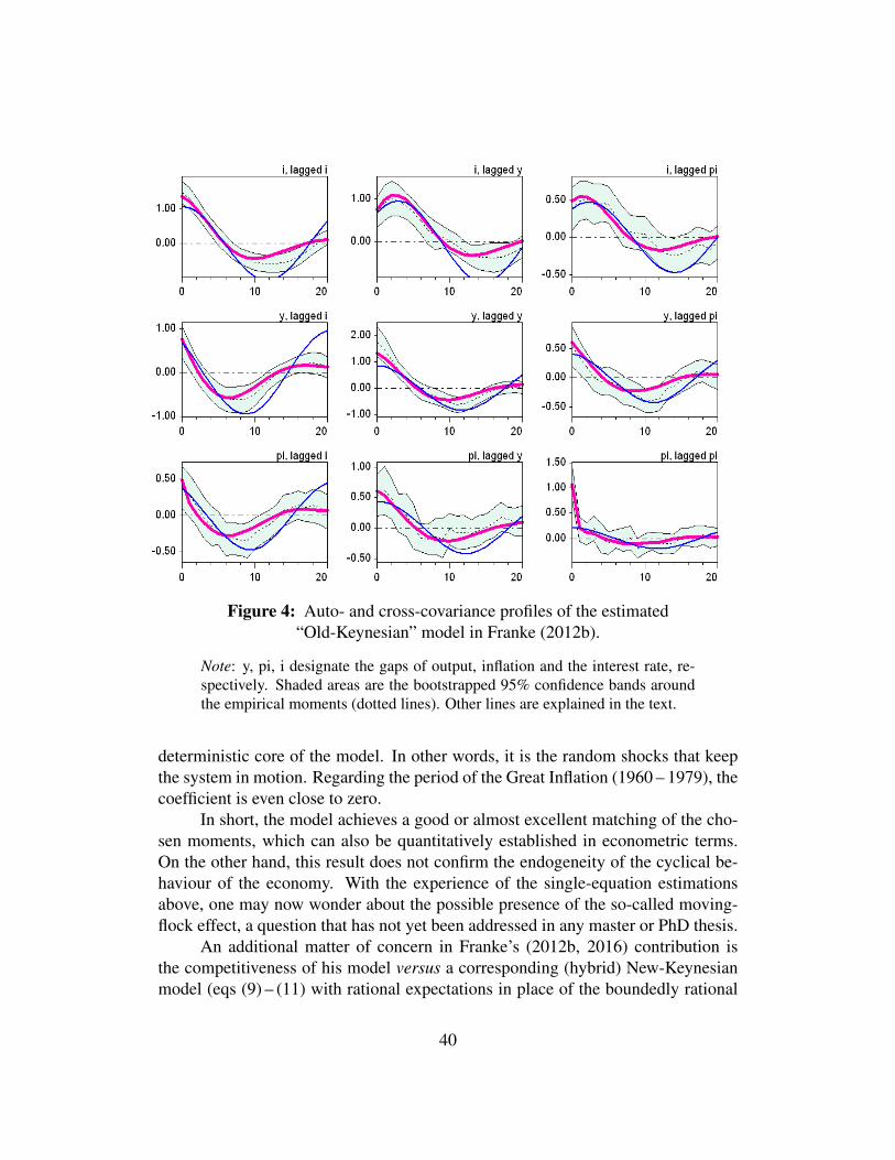
Figure 4: Auto- and cross-covariance profiles of the estimated“Old-Keynesian” model in Franke (2012b).

Note: y, pi, i designate the gaps of output, inflation and the interest rate, re-spectively. Shaded areas are the bootstrapped 95% confidence bands aroundthe empirical moments (dotted lines). Other lines are explained in the text.

deterministic core of the model. In other words, it is the random shocks that keepthe system in motion. Regarding the period of the Great Inflation (1960 – 1979), thecoefficient is even close to zero.

In short, the model achieves a good or almost excellent matching of the cho-sen moments, which can also be quantitatively established in econometric terms.On the other hand, this result does not confirm the endogeneity of the cyclical be-haviour of the economy. With the experience of the single-equation estimationsabove, one may now wonder about the possible presence of the so-called moving-flock effect, a question that has not yet been addressed in any master or PhD thesis.

An additional matter of concern in Franke’s (2012b, 2016) contribution isthe competitiveness of his model versus a corresponding (hybrid) New-Keynesianmodel (eqs (9) – (11) with rational expectations in place of the boundedly rational

40

expectations Eagg). Broadly speaking, both models are found to be equally success-ful at reproducing the autocovariances of their three state variables. If one is moreambitious, however, it has to be noted that the autocovariances and the raggednessof the inflation rate can hardly be reconciled in the New-Keynesian model: either itproduces a good match of the former and a bad match of the latter, or vice versa. Inthe Old-Keynesian model, by contrast, the two types of moments are largely com-patible, that is, a good match of one type may exist alongside at least an acceptablematch of the other type. In this sense, the Old-Keynesian model may claim to do abetter job.

Using Euro Area data and the same 78 second moments as Franke, the au-thors Jang and Sacht (2016a) estimate De Grauwe’s model (with shocks added) bythe method of simulated moments. Regarding the coefficients in the discrete choiceswitching mechanism, they argue in favour of exogenously fixing a moderate inten-sity of choice β = 1 in (13) and a zero memory coefficient ρ = 0 in (14).45 Theyfurthermore provide detailed information about several other parameters. Espe-cially the estimates of the monetary policy coefficients make good economic sense.At least to the naked eye, the matching itself is of a similar quality as in Figure4, and slightly superior to the the matching of the model’s rational expectationsversion.46

Jang and Sacht (2016b) continue this line of research. In this article, theyconsider four forecast rules (two of which with slightly more ‘momentum’ than be-fore) and alternatively include two, three or all four in the model. Together with therational expectations, they arrange a horse race for six model versions. With respectto US data and the Euro Area data, it is found in both cases that, when matchingthe same 78 moments as before, the interaction between the two new (and moredynamic) rules is almost as successful as all four rules together. In fact, insignifi-cant values for the parameters characterizing the other two rules indicate that theseare virtually ineffective. This finding supplies new knowledge in the search for ef-ficient and parsimonious specifications within the De Grauwe framework. Besides,

45Setting β = 1 is significantly superior to higher values such as 10 or 100, and insignificantlyinferior to β = 0.10. The latter would, however, undermine the philosophy of the model as thedecision between the two forecast rules is then close to tossing a coin.

46Referring to the J-test, the authors conclude that they cannot reject the null hypothesis accord-ing to which the model-generated moments may also have been obtained from the real-world datageneration process. Such an argument presupposes an optimal weighting matrix in setting up theobjective moment distance function, whereas, as mentioned by the authors (p. 89), this assumptionis not satisfied in their treatment. Nevertheless, this observation does not necessarily mean that theirconclusion is wrong, only that other methods have to be tried to address this issue; for example,repeated re-estimations of the model as discussed in Franke (2012b) and Brenneisen (2015) (seealso below).

41

the rational expectations perform the worst, which is explained by the assumptionof ruling out the lagged variables (i.e. the hybrid case) in eqs (9) and (10).

Daring to provide a brief summary of these results, at least from a higherpoint of view and as a preliminary conclusion, it seems that the model approachesby Franke and De Grauwe receive similarly good and satisfactory empirical supportfrom estimations by the method of simulated moments.

Finally, Brenneisen (2015) starts out from a recent paper by Liu and Minford(2014), who compare a purely forward-looking New-Keynesian model to a (very)simple version of De Grauwe’s model. Estimating them by indirect inference, theseauthors conclude that the former model outperforms the latter. Brenneisen pointsout a number of unclear points in Liu and Minford’s presentation and then, instead,applies the method of simulated moments to the two models—whereby he arrivesat the reverse conclusion. A more differentiated picture is obtained with respect tomoderate extensions of the models.

Very informative in Brenneisen’s contribution is a methodological issue re-garding the precision of the parameter estimates. Distributions of the parameterscan be computed by repeatedly re-estimating a model on the bootstrapped empir-ical moments, which is a sound but extremely time-consuming procedure. Theauthor successfully tests a new econometric proposal for approximating these dis-tributions by simulations of another random distribution, which can do without there-estimations completely. This alternative device is relatively easy to implementand could prove useful in future applications of the method of simulated moments.

7 Conclusion

With respect to macroeconomics, this survey was concerned with recent attempts totranslate aspects of the famous notion of the animal spirits into formal and rigorousmodelling. To cope with the ‘wilderness of bounded rationality’, two approacheswith a stylized microfoundation were addressed: the discrete choice approach andthe transition probability approach. Before discussing their applications in the lit-erature, it was revealed that they are more closely related than it might seem at firstglance, and that they are well suited to endogenously generate persistent cyclicalbehaviour.

The literature presented here shows a considerable flexibility in building mac-rodynamic models from these tools, or incorporating them into existing models. Asa first guideline for finding one’s around the many models, a distinction was offeredbetween animal spirits in a weak sense and in a strong sense. The first expressionmerely points to a rush toward one of two attitudes, strategies or similar alternatives;

42

the second involves an element of herding because, in a world of irreducible uncer-tainty, people think the majority knows better. The first variety is typically foundin models that work with the discrete choice approach. The second can primarilybe classified in models applying the transition probability approach. However, thisrole allocation is based more on historical reasons rather than on a compelling innerlogic.

Besides being theoretically attractive, the two approaches were also shown tohave some empirical support. Overall, the material and ideas discussed can providefruitful stimulations for future research that seeks to capture the formation of busi-ness or consumer sentiment, or of a general state of confidence, in a serious andstructured way. Maybe this survey comes at a good time, before further modellingwork in this direction abounds.

References

Akerlof, G.A. and Shiller, R.J. (2009): Animal Spirits. Princeton and Oxford:Princeton University Press.

Alfarano, S. and Lux, T. (2007): A noise trader model as a generator of apparentpower laws and long memory. Macroeconomic Dynamics, 11 (Supplement1), 80–101.

Anderson, S., de Palma, A. and Thisse, J. (1993): Discrete Choice Theory of Prod-uct Differentiation. Cambridge, Mass.: MIT Press.

Anufriev, M., Assenza, T., Hommes, C. and Massaro, D. (2013): Interest rate rulesand macroeconomic stability under heterogeneous expectations. Macroeco-nomic Dynamics, 17, 1574–1604.

Anufriev, M., Bao, T. and Tuinstra, J. (2016): Microfoundations for switching be-havior in heterogeneous agent models: An experiment. Journal of EconomicBehavior and Organization, 129, 74–99.

Anufriev, M. and Hommes, C. (2012a): Evolutionary selection of individual ex-pectations and aggregate outcomes in asset pricing experiments. AmericanEconomic Journal: Microeconomics, 4:4, 35–64.

Anufriev, M. and Hommes, C. (201ba): Evolution of market heuristics. The Knowl-edge Engineering Review, 27, 255–271.

Assenza, T., Bao, T., Hommes, C. and Massaro, D. (2014a): Experiments on ex-pectations in macroeconomics and finance. In J. Duffy (ed.), Experiments inMacroeconomics (Research in Experimental Economics, Volume 17). Emer-

43

ald Group Publishing Limited; pp. 11–70.(http://dx.doi.org/10.1108/S0193-230620140000017002)

Assenza, T., Heemeijer, P., Hommes, C. and Massaro, D.(2014b): Managing self-organization of expectations through monetary policy: A macro experiment.CeNDEF, University of Amsterdam, Working Paper 2014-07.

Bernanke, B.S., Gertler, M. and Gilchrist, S. (1999): The financial accelerator ina quantitative business cycle framework. In Taylor, J.B. and Woodford, M.(Eds.), Handbook of Macroeconomics, Vol. 1. Amsterdam: North-Holland;pp. 1342–93.

Boyd, I. and Blatt, J.M. (1988): Investment, Confidence and Business Cycles. NewYork: Springer.

Branch, W. (2004): The theory of rationally heterogeneous expectations: Evidencefrom survey data on inflation expectations. Economic Journal, 114, 592–621.

Branch, W. (2007): Sticky information and model uncertainty in survey data oninflation expectations. Journal of Economic Dynamics and Control, 31, 245–276.

Branch, W.A. and Evans, G.W. (2011): Monetary policy and heterogeneous expec-tations. Economic Theory, 47, 365–393.

Branch, W.A. and McGough, B. (2009): A New Keynesian model with heteroge-neous expectations. Journal of Economic Dynamics and Control, 33, 1036–51.

Branch, W.A. and McGough, B. (2010): Dynamic predictor selection in a newKeynesian model with heterogeneous expectations. Journal of Economic Dy-namics and Control, 34, 1492–1508.

Brazier, A., Harrison, R., King, M. and Yates, T. (2008): The danger of inflating ex-pectations of macroeconomic stability: Heuristic switching in an overlapping-generations monetary model. International Journal of Central Banking, 4:2,219–254.

Brenneisen, J.-N. (2015): Moment matching of heterogeneous expectations in aclass of recent macroeconomic business cycle models. Unpublished masterthesis, University of Kiel.

Brock, W.A. and Durlauf, S.N. (2001): Discrete choice with social interactions.Review of Economic Studies, 68, 235–260.

Brock, W.A. and Hommes, C.H. (1997): A rational route to randomness. Econo-metrica, 65, 1059–1095.

44

Brock, W.A. and Hommes, C.H. (1998): Heterogeneous beliefs and routes to chaosin a simple asset pricing model. Journal of Economic Dynamics and Control,22, 1235–1274.

Chiarella, C. and Di Guilmi, C. (2015): The limit distribution of evolving strategiesin financial markets. Studies in Nonlinear Dynamics and Econometrics, 19:2,137–159.

Cochrane, J.H. (2001): Asset Pricing. Princeton: Princeton University Press.Cornea-Madeira, A., Hommes, C. and Massaro, D. (2015): Behavioral heterogene-

ity in U.S. inflation dynamics. CeNDEF, University of Amsterdam, WorkingPaper.

Da Silveira, J.J. and Lima, G.T. (2014): Heterogeneity in inflation expectations andmacroeconomic stability under satisficing learning. Working Paper 2014-28,FEA/USP Sao Paulo.

De Grauwe, P. (2008a): DSGE-modelling when agents are imperfectly informed.ECB, Working Paper Series No. 897.

De Grauwe, P. (2008b): Stock prices and monetary policy. Centre for EuropeanPolicy Studies, Working Document No. 304.

De Grauwe, P. (2010): Top-down versus bottom-up macroeconomics. CESifoWorking Paper No. 3020.

De Grauwe, P. (2011): Animal spirits and monetary policy. Economic Theory, 47,423–457.

De Grauwe, P. (2012a): Booms and busts in economic activity: A behavioral ex-planation. Journal of Economic Behavior and Organization, 83, 484–501.

De Grauwe, P. (2012b): Lectures on Behavioral Macroeconomics. Princeton: Prince-ton University Press.

De Grauwe, P. and Gerba, E. (2015a): Stock market cycles and supply side dynam-ics: Two worlds, one vision? CESifo Working Paper No. 5573.

De Grauwe, P. and Gerba, E. (2015b): Monetary transmission under competingcorporate finance regimes. London School of Economics, FinMaP-WorkingPaper, No. 52.

De Grauwe, P. and Macchiarelli, C. (2015): Animal spirits and credit cycles. Jour-nal of Economic Dynamics and Control, 59, 95–117.

Diks, C. and van der Weide, T. (2005): Herding, a-synchronous updating and het-erogeneity in memory in a CBS. Journal of Economic Dynamics and Control,29, 741–762.

45

Drager, L. (2016): Recursive inattentiveness with heterogeneous expectations. Ma-croeconomic Dynamics, 20, 1073–1100.

Drager, L. (2011): Endogenous persistence with recursive inattentiveness. Uni-versity of Hamburg, DEP Discussion Papers Macroeconomics and FinanceSeries 3/2011.

Drager, L. (2010): Why don’t people pay attention? Endogenous sticky informationin a DSGE Model. University of Hamburg, DEP Discussion Papers Macro-economics and Finance Series 2/2010.

Farmer, R. and Guo, J.T. (1994): Real business cycles and the animal spirit hypoth-esis. Journal of Economic Theory, 63, 42–72.

Flaschel, P., Franke, R. and Semmler, W. (1997): Dynamic Macroeconomics: Insta-bility, Fluctuations, and Growth in Monetary Economies. Cambridge, Mass:MIT Press.

Franke R. (2016) Competitive moment matching of a New-Keynesian and an Old-Keynesian model. Journal of Economic Interaction and Coordination (forth-coming).

Franke, R. (2014): Aggregate sentiment dynamics: A canonical modelling ap-proach and its pleasant nonlinearities. Structural Change and Economic Dy-namics, 31,64–72.

Franke, R. (2012a): Microfounded animal spirits in the new macroeconomic con-sensus. Studies in Nonlinear Dynamics and Econometrics, vol. 16, issue 4.

Franke R. (2012b) Competitive moment matching of a New-Keynesian and an Old-Keynesian model: Extended version. Working paper, University of Kiel.(http://www.gwif.vwl.uni-kiel.de/en/ working-papers).

Franke, R. (2008a): Microfounded animal spirits and Goodwinian income distrib-ution dynamics. In: Flaschel, P. and Landesmann, M. (eds.), Effective De-mand, Income Distribution and Growth. Research In Memory of the Work ofRichard M. Goodwin. London: Routledge; pp. 372–398.

Franke, R. (2008b): Estimation of a microfounded herding model on German sur-vey expectations. Intervention: European Journal of Economics and Eco-nomic Policies, 5, 301–328.

Galı, J. (1994): Monopolistic competition, business cycles, and the composition ofaggregate demand. Journal of Economic Theory, 63, 73–96.

Ghonghadze, J. (2016): Variation of lending terms and the financial instability hy-pothesis. Working paper, University of Kiel.

46

Goodwin, R.M. (1967): A growth cycle model. In C.H. Feinstein (ed.), Socialism,Capitalism and Growth. Cambridge: Cambridge University Press.

Haag, G., Weidlich, W. and Mensch, G. (1987): The Schumpeter clock. In D. Battenet al. (eds), Economic Evolution and Structural Adjustment. Berlin: Springer.

Hohnisch, M. and Westerhoff, F. (2010): Consumer sentiment and countercyclicalfiscal policies. International Review of Applied Economics, 24, 609–618.

Hohnisch, M. and Westerhoff, F. (2008): Business cycle synchronization in a sim-ple Keynesian macro-model with socially transmitted economic sentimentand international sentiment spill-over. Structural Change and Economic Dy-namics, 19, 249–259.

Hommes, C.H., Huang, H. and Wang, D. (2005): A robust rational route to ran-domness in a simple asset pricing model. Journal of Economic Dynamicsand Control, 29, 1043–1072.

Jang, T.-S. and Sacht, S. (2016a): Animal spirits and the business cycle: Empiricalevidence from moment matching. Metroeconomica, 67, 76–113.

Jang, T.-S. and Sacht, S. (2016b): Modelling consumer confidence and its role forexpectation formation: A horse race. Working paper, Kyungpook NationalUniversity and University of Kiel.

Keynes, J.M. (1936): The General Theory of Employment, Interest and Money.London: Macmillan.

Keynes, J.M (1937): The general theory of employment. Quarterly Journal ofEconomics, 51, 109–123.

Kirman, A. (1991): Epidemics of opinion and speculative bubbles in financial mar-kets. In M. Taylor (ed.), Money and Financial Markets. Cambridge: Black-well; pp. 354–368.

Kirman, A. (1993): Ants, rationality and recruitment. Quarterly Journal of Eco-nomic, 108, 137–156.

Kraft, P., Landes, T. and Weise, P. (1986): Dynamic aspects of a stochastic businesscycle model. Methods of Operations Research, 53, 445–453.

Lahkar, R. and Sandholm, W.H. (2008): The projection dynamic and the geometryof population games. Games and Economic Behavior, 64, 565–590.

Lengnick, M. and Wohltmann, H.-W. (2013): Agent-based financial markets andNew Keynesian macroeconomics: A synthesis. Journal of Economic Inter-action and Coordination, 8, 1–32.

Lengnick, M. and Wohltmann, H.-W. (2016): Optimal monetary policy in a new

47

Keynesian model with animal spirits and financial markets. Journal of Eco-nomic Dynamics and Control, 64, 148–165.

Lines, M. and Westerhoff, F. (2012): Effects of inflation expectations on macro-economic dynamics: Extrapolative versus regressive expectations. Studies inNonlinear Dynamics and Econometrics, Vol. 16, Issue 4, Article 7.

Lines, M. and Westerhoff, F. (2010): Inflation expectations and macroeconomicdynamics: The case of rational versus extrapolative expectations. Journal ofEconomic Dynamics and Control, 34, 246–257.

Lines, M. and Westerhoff, F. (2006): Expectations and the multiplier-acceleratormodel. In: T. Puu and I. Sushko (eds): Business Cycles Dynamics. Modelsand Tools. Springer: Berlin, pp. 255–276.

Liu, C. and Minford, P. (2014): Comparing behavioural and rational expectationsfor the US post-war economy. Economic Modelling, 43, 407–415.

Lojak, B. (2016): Sentiment-driven investment, non-linear corporate debt dynamicsand co-existing business cycle regimes. BERG Working Paper Series No.112, University of Bamberg.

Lojak, B. (2015): Investor sentiment, corporate debt and inflation in a feedback-guided model of the business cycle. Unpublished master thesis, University ofKiel.

Lux, T. (1995): Herd behaviour, bubbles and crashes. Economic Journal, 105,881–889.

Lux, T. (2009): Rational forecasts or social opinion dynamics: Identification ofinteraction effects in a business climate index. Journal of Economic Behaviorand Organization, 72, 638–655.

Mankiw, N.G. and Reis, R. (2002): Sticky information versus sticky prices: Aproposal to replace the New Keynesian Phillips curve. Quarterly Journal ofEconomics, 117, 1295–1328.

Manski, C. and McFadden, D. (1981): Structural Analysis of Discrete Data WithEconometric Applications. Cambridge, Mass.: MIT Press.

Massaro, D. (2013): Heterogeneous expectations in monetary DSGE models. Jour-nal of Economic Dynamics and Control, 37, 680–692.

Metzler, L.A. (1941): The nature and stability of inventory cycles. Review of Eco-nomics and Statistics, 23, 113–129.

Minsky, H.P. (1975): John Maynard Keynes. New York: Columbia UniversityPress.

48

Ochea, M. (2010): Essays on Nonlinear Evolutionary Game Dynamics. PhD thesis,University of Amsterdam: Book no. 468 of the Tinbergen Institute ResearchSeries.

Samuelson, P. (1939): Interactions between the multiplier analysis and the principleof acceleration. Review of Economic Statistics, 21,75–78.

Scheffknecht, L. and Geiger, F. (2011): A behavioral macroeconomic model withendogenous boom-bust cycles and leverage dynamics. FZID Discussion Pa-per 37-2011, University of Hohenheim.

Wegener, M. and Westerhoff, F. (2012): Evolutionary competition between predic-tion rules and the emergence of business cycles within Metzlers inventorymodel. Journal of Evolutionary Economics, 22, 251–273.

Wegener, M., Westerhoff, F. and Zaklan, G. (2009): A Metzlerian business cyclemodel with nonlinear heterogeneous expectations. Economic Modelling, 26,715–720.

Weidlich, W. and Braun, M. (1992): The master equation approach to nonlineareconomics. Journal of Evolutionary Economics, 2, 233–265.

Weidlich, W. and Haag, G. (1983): Concepts and Models of a Quantitative Sociol-ogy. The Dynamics of Interacting Populations. Berlin: Springer.

Weise, P. and Kraft, M. (1988): Cumulative processes, disproportionalities, andSpiethoff’s theory of the business cycle. In P. Flaschel and M. Kruger (eds),Recent Approaches to Economic Dynamics. Frankfurt a.M.: P. Lang; pp. 3–16.

Westerhoff, F. (2010): An agent-based macroeconomic model with interacting firms,socio-economic opinion formation and optimistic/pessimistic sales expecta-tions. New Journal of Physics, Vol. 12, 075035.

Westerhoff, F. (2008): Heuristic expectation formation and business cycles: A sim-ple linear model. Metroeconomica, 59, 47–56.

Westerhoff, F. (2006a): Samuelson’s multiplier-accelerator model revisited. Ap-plied Economics Letters, 13, 89–92.

Westerhoff, F. (2006b): Nonlinear expectation formation and endogenous businesscycles. Studies in Nonlinear Dynamics and Econometrics, Vol. 10, Issue 4,Article 4.

Westerhoff, F. (2006c): Business cycles, heuristic expectation formation and con-tracyclical policies. Journal of Public Economic Theory, 8, 821–838.

49

Westerhoff, F. and Hohnisch, M. (2007): A note on interactions-driven businesscycles. Journal of Economic Interaction and Coordination, 2, 85–91.

Yanovski, B. (2014): Introducing an elementary microstructure into macrodynamicmodels. Unpublished master thesis, University of Kiel.

50