AGH - UNIVERSITY OF SCIENCE AND TECHNOLOGY FACULTY OF NON-FERROUS METALS

Department of Theoretical Metallurgy and Metallurgical Engineering

Ph.D. THESIS

Title: MINIMIZATION OF ENTROPY GENERATION IN STEADY

STATE PROCESSES OF DIFFUSIONAL HEAT AND MASS TRANSFER

Author: Mgr Jacek Mikołaj Łatkowski

Supervisor: Prof. zw. dr hab. inż. Zygmunt Kolenda

KRAKÓW, NOVEMBER 2006

2

Pozwalam sobie wyrazić serdeczne podziękowanie

Profesorowi Zygmuntowi Kolendzie za cenne rady i za kierownictwo naukowe mojej pracy doktorskiej

I would like to express my sincere gratitude to Professor Zygmunt Kolenda, for his guidance and support during the completion of the thesis.

3

Table of Content 1. Introduction 7

2. Description of the thermodynamics of the non-equilibrium processes of mass and energy transfer – literature overview 8

2.1 Theoretical background 8

2.2 Calculation of entropy production 12

2.3 Examples of phenomenological description 17

2.3.1 Heat conduction and electric current flow 17

2.3.2 Thermal diffusion 19

2.4 Irreversible, stationary process of heat conduction 20

2.5 The principle of minimum entropy production in stationary states 23

2.6 Principle of entropy production compensation 26

3. Aims of the thesis 29

4. Minimization of entropy production and principle of entropy production compensation in steady state linear processes of diffusional mass and energy transfer 33

4.1 Heat conduction in a plane-wall 33

4.2 Diffusional mass transfer 39

5. Entropy production minimization in stationary processes of heat and electric current flows 42

5.1 Non-linear boundary problem without the internal heat source 45

5.2 Boundary problem with boundary conditions of the third kind (Sturm-Liouville boundary conditions) without internal heat source 45

5.3 Boundary problem with simultaneous heat and electric current flows 49

5.4 Methods of calculation of additional internal heat source and entropy generation rate 51

4

6. Methods of solving the boundary problems with Euler-Lagrange equations 61

6.1 General method of determining the internal heat source and entropy generation rate 61

7. Solutions for the specific boundary problems 68

7.1 Simultaneous heat and electric current flows 68

7.2 Boundary conditions of the second and third kinds - heat conduction coefficient independent of temperature 87

7.3 Boundary conditions of the third kind (Sturm-Liouville boundary conditions) - heat conduction coefficient dependent on temperature 92

8. Applications 96

9. Summary 98

Appendix 1 100

References 102

5

Symbols A - chemical affinity A, B - integration constants Ci - concentration of i-th component ci - integration constants deS - entropy exchange with surroundings diS - entropy production due to irreversibility DT - thermal diffusion coefficient Dd - Dufour coefficient F - Helmholtz free energy F - thermodynamic force F - function G - Gibbs free energy H - enthalpy h - heat transfer coefficient I,i - density of electric current J - thermodynamic flux Jk - mass flux of k-th component Jq - heat flux Js - entropy flux Ju - internal energy flux k - thermal conductivity coefficient kf - thermal conductivity coefficient of fluids Lik - phenomenological coefficients n - normal to the surface ni - number of moles of i-th component p - pressure

q& - heat flux

vq& - internal heat source

Q& - heat flow Q - heat

sT - Soret coefficient S - entropy of the system s - specific entropy

6

T - absolute temperature or dimensionless temperature Tf - fluid temperature (absolute or dimensionless) u - specific internal energy U - internal energy v - specific volume V - volume W - work X - thermodynamic force x, y ,z - cartesian coordinates Greek symbols δ - change μi - chemical potential of i-th component νi - stoichiometric coefficient νik - stoichiometric coefficient of the k-th component for the i-th chemical reaction ξ - extent of reaction ρ - density ρ - specific electric resistivity σ - entropy generation rate (entropy production) τ - time Γ - boundary surface Φ - function Ψ - electric potential

7

1. Introduction

Progress of the human civilization is intrinsically connected with the use of energy sources. Methods of harnessing the natural energy resources can be better or worse, more or less effective, cost-conscious or unlimited. It is rather obvious that we are trying for those methods to be better, more effective and cost-cutting. These aims are primarily reached through the development of scientific research and in the topics discussed in this thesis, through the applications of methods of non-equilibrium thermodynamics. The main problem, widely discussed during the last decade, is the issue of diminishing natural resources, specially the energy resources.

The problem of diminishing energy resources was first discussed in a well

known report “Limits of progress” (Meadows and others, 1972). The authors of the report, using various mathematical models, formulated the hypothesis that in the middle of the 21st century there will be a collapse in the development of rich countries as the result of the overexploitation of the natural resources. We know well today that those catastrophic predictions have not been confirmed. In addition to economic problems, we face today the dangers of excessive pollution and irreversible destruction of the natural environment as the result of increasing demand for nonrenewable energy resources. Negative consequences of global warming as an effect of human activity are the prime example.

Thus, we can ask the question – are the dangers of our civilization’s progress real as the effect of diminishing natural resources, especially fuel resources. This question is based on the premise that non-renewable natural resources are gone. However, the optimistic is the fact that natural energy resources can be replaced by other renewable sources of primary energy or nuclear energy, which at the current progress of technology, could become the sources of unlimited energy.

Even, considered negative, population growth does not seem to be a threat

since each new human being is born with the ability to be creative. It seems as well that the accumulated use of energy in the industrial countries allows for the fast progress in technology which in turn results in a decrease of irrational use of resources.

The following thesis is about the solutions which lead to the decrease in

the exploitation of natural resources and to limiting the dangers to the natural environment.

8

2. Description of the thermodynamics of the non-equilibrium processes of mass and energy transfer – literature overview

In this chapter the fundamental terminology of the non-equilibrium thermodynamic processes has been presented. The expression describing the entropy production (entropy generation rate) has been derived as the measure of intensity of the irreversible process. The principle of entropy production compensation has been discussed as the basis for minimizing entropy production. The main non-equilibrium processes and their links have also been discussed. 2.1 Theoretical background

The fundamental relationship resulting from the classical thermodynamics, known as the Clausius’ inequality, describes the change of entropy dS of the thermodynamic system in the form:

đQdST

≥

(2.1)

where đQ is the elementary heat exchanged between the system and the environment and T is the local temperature (relation (2.1) has a local character). Relation (2.1) can also be written in the form:

0T dS đQ− ≥ (2.2)

Inequality sign in (2.1) and (2.2) describes the irreversible processes while the equality is required for the idealized equilibrium or reversible processes. Deriving , as done by T. de Donder [2], the term for non-compensated heat

đQ T dS đQ= − (2.3)

the Second Law of Thermodynamics can be written as:

0đQ ≥

9

As the result of de Donder’s analysis, non-compensated heat is the measure of spontaneity of the process which consequently leads to general definition of chemical affinity A for the spontaneous chemical reaction:

đQAdξ

=

where dξ = dni /νi is called the extent of a reaction, dni is the elementary change in number of moles of the particular component in the reaction while iν is the stoichiometric coefficient. In case when the system is doing only the mechanical work, the formulation of the First Law of Thermodynamics gives:

đQ dU pdV= + (2.4)

where dU is the elementary change of internal energy, p is the pressure and dV is the elementary change of volume of the system. Combining equations (2.3) and (2.4) results in:

dU TdS pdV đQ= − − Introducing, from the definitions the expressions for: enthalpy H: H = U + pV Helmholtz free energy: F = U – TS Gibbs free energy: G = H – TS, we receive the following set of equations:

dU TdS TdV AddH TdS Vdp AddF SdT pdV AddG SdT VdP Ad

ξξξξ

= − −= + −= − −= + −

(2.5)

10

Expression (2.3) can be further changed into the expression:

đQ đQdST T

= +

(2.6) From the definitions

eđQd ST

=

and (2.7)

iđQd ST

=

(2.8) equation (2.6) becomes:

e idS d S d S= + (2.9)

Since

đQdST

≥

then

edS d S≥ (2.10)

which means that always:

diS ≥ 0 (2.11)

where: diS > 0 for irreversible processes

diS = 0 for reversible processes

11

From equation (2.6) we can see that eđQd ST

= describes the exchange of

entropy between the system and the surroundings and iđQd ST

= is the entropy

production due to irreversible processes inside the system. In the analysis of expression for diS, significant role is played by the local formulation of the Second Law of Thermodynamics. It states that in every microscopic part of the system in which irreversible processes take place, the entropy production (entropy generation rate) diS/dτ, where τ is the time, must be positive or:

0id Sdτ

>

(2.12) It means as well that in a given volume, there can simultaneously take place processes with positive and negative entropy production but in such a way that the positive entropy production is greater from the negative production (within the absolute value), which insures the validity of inequality (2.12). Differentiating equation (2.9) gives:

e id S d SdSd d dτ τ τ

= +

(2.13) where dS/dτ is the entropy rate of change of the system as the result of the entropy rate of exchange with the surroundings dSe/dτ and the entropy production (entropy generation rate) is

id Sd

στ

=

(2.14) The general differential equation of the local entropy for any irreversible closed system is:

sds divJd

ρ στ= − +

(2.15) and

12

( )sds div J svd

ρ ρ στ= − + +

(2.16) for the open system, where s represents the entropy value per unit volume , ρ – the density of the substance, Js – entropy flow (entropy flux) exchanged with the surroundings and v is the flow velocity. The most important element, in the analysis of irreversible processes, is the calculation of entropy production (rate of entropy production). This value directly describes the level of irreversibility of the given process. It is important to mention as well that the entropy production is path dependant and should not be confused with entropy change. The condition:

0id Sd

στ

= ≥

(2.17)

directly indicates that, for example, the process along two different paths A and B such that

A Bσ σ> (2.18)

means that path A is more irreversible than path B. 2.2 Calculation of entropy production

The method of calculating the amount of entropy production related to different irreversible processes, is based on the entropy balance equations. For example, equation (2.15) yields:

sds Jd

στ

= + ∇ ⋅r

(2.19)

13

Neglecting the kinetic energy dissipation and with no external fields, Gibbs relation:

k kk

T ds du dnμ= − ∑

(2.20) where μk is the specific thermodynamic potential for the k-th component of the system while dnk represents the elementary change of the amount of the k-th component, leads to:

1 k k

k

ns uT T

μτ τ τ

∂∂ ∂= −

∂ ∂ ∂∑

(2.21) Introducing the mole-number balance equation for the amount of the k-th component,

kk jk j

j

n J ν υτ

∂= −∇ ⋅ +

∂ ∑r

(2.22) where νik is the stoichiometric coefficient of k-th component for the j-th chemical reaction and υj is the rate of the j-th reaction in volume V,

1 jj

dV d

ξυ

τ=

and the equation of the First Law of Thermodynamics:

0uu Jτ

∂+ ∇ ⋅ =

∂

r

(2.23) where Ju is the internal energy flux, equation (2.21) takes the following form:

,

1 k ku k jk j

k k j

s J JT T T

μ μν υ

τ∂

=− ∇⋅ + ∇⋅ −∂ ∑ ∑

r r

(2.24)

Introducing from definition,

14

j k jkk

A μ ν= −∑

equation (2.24) becomes,

1 j ju k k ku k

k k j

AJ Js J JT T T T T

υμ μτ

⎛ ⎞∂+∇⋅ − = ⋅∇ − ⋅∇ +⎜ ⎟∂ ⎝ ⎠

∑ ∑ ∑r r

r r

(2.25) where the following property was used for the scalar function g and vector J,

( ) ( )g J J g g J∇⋅ = ⋅∇ + ∇⋅r r r

Comparing equation (2.25) with the entropy balance equation (2.19) leads to the expression:

u k ks

k

J JJT T

μ⎛ ⎞= −⎜ ⎟⎝ ⎠

∑r r

r

(2.26) and the expression for entropy production:

1 0j jku k

k j

AJ J

T T Tυμ

σ = ⋅∇ − ⋅∇ + ≥∑ ∑r r

(2.27) In case of the external electric field with the electric field strength E ψ= −∇ (ψ – electric potential) resulting in the flow of electrical current with the current density I, the following equation is derived

( )1 j jku k

k j

AIJ J

T T T Tυψμσ

⋅ −∇= ⋅∇ − ⋅∇ + +∑ ∑

rr r

(2.28)

15

The derived equation (2.28) is the general expression for the entropy production in which four irreversible processes were taken into account: heat conduction, mass diffusion, electric current flow and chemical reactions. Mathematical structure of equations (2.27) and (2.28) indicates that they be both written in the general form:

k kk

F Jσ = ∑

(2.29) where Fk is called the thermodynamic force and Jk – the thermodynamic flow, coupled with forces. For the processes discussed above, the forces and flows are listed in Table 1. Table 2.1 Forces and flows in entropy generation equations Irreversible Process Force Fk Flow Jk Heat Conduction 1

T⎛ ⎞∇ ⎜ ⎟⎝ ⎠

Heat flow Ju

Diffusion k

Tμ

−∇ Diffusion current Jk

Electric current flow ET Tψ

−∇ =r

Current density I

Chemical reaction jAT Reaction rate

1 jj

dV d

ξυ

τ=

Equations (2.27) and (2.28) play a fundamental role in determining the entropy production for the processes with known thermodynamic forces and flows. In general, the amount of entropy production is calculated from the mathematical models for the processes being considered. In case of cross effects, for example simultaneous heat conduction and electric current flow, the entropy production is described, with a good accuracy, by the linear relationship between flows and thermodynamic forces, in the form:

k kj jj

J L F= ∑

(2.30)

16

where Lkj is called phenomenological coefficients, whose values can be found experimentally. Substituting equation (2.30) into equation (2.29), the entropy production takes the quadratic form:

,0jk j k

j kL F Fσ = >∑

(2.31) Because of positive sign of entropy production, a matrix Ljk is said to be positive definite. This means that the two-dimensional matrix Ljk,

11 12

21 22

L LL L

is positive definite if the following conditions are satisfied:

L11 > 0, L22 > 0 and (L12+L21)2 < 4L11L22 In general, for the matrix

11 12 1

21 22 2

1 2

.......................

:...........

n

n

n n nn

L L LL L L

L

L L L

=

there are following conditions: Lkk > 0 for k ε < 1, n > and all the main minors are positive definite. In 1931, Lars Onsager introduced the principle of symmetry of matrix L. This means that for the linearly independent forces and flows, the following relations hold true:

Ljk = Lkj (2.32)

These relations are sometimes known as the Fourth Law of Thermodynamics.

17

2.3 Examples of phenomenological description

In the following sections, the phenomenological description of several cross effects such as heat conduction and electric current flow as well as thermal diffusion will be presented in detail. 2.3.1 Heat conduction and electric current flow This phenomena is known as thermoelectric effect and its general description is shown in Figure 1. ΔΨ I → Al Al Cu Cu Jq→ T T+ΔT T T Seebeck Effect Peltier Effect - ΔΨ/ΔT Π=Jq/I Fig. 2.1 Thermoelectric effect Phenomenological equations are as follows:

1

1

q qq qe

e ee eq

EJ L LT T

EI L LT T

⎛ ⎞= ∇ +⎜ ⎟⎝ ⎠

⎛ ⎞= + ∇ ⎜ ⎟⎝ ⎠

rr

rr

(2.33)

where index q and e relate to heat flow and current density. According to Onsager’s principle:

Lqq > 0 , Leq > 0 and Lee=Lqe After rearrangement, equations (2.33) become

18

2

2

1

1

q qq qe

e ee eq

T EJ L LT x T

E TI L LT T x

∂= − +

∂∂

= −∂

rr

rr

(2.34)

Comparing expression

2

1qq

TLT x

∂−

∂

with the Fourier’s law leads to the relation:

2qqL

kT

=

(2.35) which for the known coefficient of heat conduction k, allows for calculation of Lqq. In a similar way, another relation can be derived:

eeTLρ

=

(2.36) where ρ is the specific electric resistance and

0eq ee

T

L L TTψ

=

Δ⎛ ⎞= − ⎜ ⎟Δ⎝ ⎠

(2.37) where Δψ/ΔT is the Seebeck’s coefficient determined experimentally similarly to

qe eeL L= Π (2.38)

where 0

q

e T

JI

Δ =

⎛ ⎞Π = ⎜ ⎟

⎝ ⎠ is the Peltier’s coefficient.

19

2.3.2 Thermal Diffusion

The interaction between heat and mass flows produces two effects known as the Soret effect and the Dufour effect. The equation for entropy production has the form:

( ) ,1 k T pq k

kJ J

T T

μσ

∇⎛ ⎞= ⋅∇ − ⋅⎜ ⎟⎝ ⎠

∑r

(2.39)

For the two component system, the following relations are obtained:

1 1 11 12

2 2 1

1 1 1 11 11 12

2 2 1

1 1

1 1

qqq q

q

L nJ T L nT T n n

L nJ T L nT T n n

ν μν

ν μν

⎛ ⎞ ∂= − ∇ − + ∇⎜ ⎟ ∂⎝ ⎠

⎛ ⎞ ∂= − ∇ − + ∇⎜ ⎟ ∂⎝ ⎠

(2.40) where n and ν mean accordingly the number of moles in the substance and the partial molar volume. This allows to determine the diffusion and heat conduction coefficients:

1 1 11 11

2 2 1

2

1 1

qq

nD LT n n

Lk

T

ν μν

⎛ ⎞ ∂= +⎜ ⎟ ∂⎝ ⎠

=

(2.41) From the Onsager’s principle,

Lq1 = L1q

Introducing the general coefficient of thermal diffusion

20

12

1

1qT

L TD

T n T∇

=∇

the Soret coefficient becomes:

12

1 1 1

qTT

LDsD D T n

= =

(2.42) and the Dufour coefficient is:

1 1 11

1 2 2 1

1 1d qnD L

n T n nν μν

⎛ ⎞ ∂= +⎜ ⎟ ∂⎝ ⎠

(2.43) The values of coefficient sT and Dd are determined experimentally what allows for the calculation of phenomenological coefficient Lq1. Many examples of the applications of linear thermodynamics for irreversible processes can be found in literature [2]. 2.4 Irreversible, stationary process of heat conduction

An important group of irreversible processes is represented by stationary states. Stationary state is reached by the system when the imposed thermodynamic forces are constant (independent of time) and this state is characterized by the constant entropy production. As an example, stationary state for heat conduction has been discussed. The schematic diagram (infinite plane-wall) and the geometry of the process are shown in Figure 2. The heat flows spontaneously from the source with the higher temperature TH to a source with a lower temperature TL. The coefficient of thermal conduction of the plane-wall is constant.

21

T

Hh →∞

- Lh →∞ k TH

qJr

fluid flow fluid flow kk with temp. TL

with temp. TL TH x 0 L Fig. 2.2 Boundary value problem of the first kind Since the heat conduction is the only irreversible process, therefore the entropy production is

1qJ

Tσ = ⋅∇

r

(2.44) If the temperature gradient is only in x direction, the entropy production per unit length is given by

21 1 ( )( )( )q q

T xx J Jx T x T x

σ⎛ ⎞∂ ∂

= = −⎜ ⎟∂ ∂⎝ ⎠

(2.45) The total entropy production is therefore

0 0

1( )L L

it q

d S x dx J dxd x T

σ στ

∂ ⎛ ⎞= = = ⎜ ⎟∂ ⎝ ⎠∫ ∫

(2.46)

qJr

k = constant

22

In case of the stationary state, 0Tt

∂=

∂ and qJ

r is constant. The stationary state

also implies that the total entropy of the system is constant:

0e id S d Sd Sd d dτ τ τ

= + =

which means that:

e id S d Sd dτ τ

= −

Integrating equation (2.46) gives

0 0

1 0( )

LLq q qi

qC H

J J Jd S J dxd x T x T T Tτ

⎛ ⎞∂= = = − >⎜ ⎟∂ ⎝ ⎠∫

so

, ,i

s out s ind S J Jdτ

= −

(2.47) where Js is the entropy flow.

In general:

is

d S div Jdτ

=

(2.48) Identical equations describe the mass diffusion while the temperature T is replaced by the concentration of the k-th component of the substance.

23

2.5 Principle of minimum entropy production for stationary states

The expression

k kk

F Jσ = ∑

which describes the entropy production σ for irreversible processes, shows how different thermodynamic flows Jk are coupled with the corresponding thermodynamic forces Fk. Let some forces Fk, (k=1,2,…..,m) to be at a fixed nonzero value, while leaving the remaining forces Fk, (k=m+1, …..n), free. In stationary state the thermodynamic flows corresponding to the constrained forces reaching a nonzero constant (k = 1,2,…..m), Jk=constant, whereas the other flows are equal to zero, Jk=0, (k=m+1,…..n). Prigogine [2] has revealed the truthfulness of the following principle: “In a linear regime, the total entropy production in a system subject to flow of energy and matter, /id S d dVτ σ= ∫ reaches a minimum value at the non-equilibrium stationary state”. Mathematically,

minimumit

V

d S dVd

σ στ

= = ⇒∫

(2.49) Such a general criterion was first formulated by Lord Rayleigh as the “principle of least dissipation of energy”. Consider, for example, a system with two forces and flows that are coupled. The total entropy production is:

( )1 1 2 2i

tV

d S F J F J dVd

στ

= = +∫

24

Let the force F1 remain at a fixed nonzero value. In addition, in a stationary state, J1=constant ≠ 0 and J2 = 0 .The linear phenomenological relations of flows and forces give:

1 11 1 12 2

2 21 1 22 2 0J L F L FJ L F L F

= += + =

Using Onsager’s reciprocal relations L21=L12, the total entropy production becomes:

( )2 211 1 12 1 2 22 22t

V

L F L F F L F dVσ = + +∫

In follows from the Prigogine’s principle that σ reaches minimum when:

( )22 2 12 12

2 0V

L F L F dVFσ∂

= + =∂ ∫

(2.50) where F2 is the free force. The entropy production is minimized when the integrand expression in (2.50) is equal to zero, that is

2 2 1 1 2 2 2 0J L F L F= + = . This result can easily be generalized to an arbitrary number of forces and flows. Consider the boundary problem of the first kind shown in Figure 2.2. For the one dimensional heat flow, entropy production is given by equation (2.46):

0 0

1( )L L

it q

d S x dx J dxd x T

σ στ

∂ ⎛ ⎞= = = ⎜ ⎟∂ ⎝ ⎠∫ ∫

Introducing expression:

1q qqJ L

x T∂ ⎛ ⎞= ⎜ ⎟∂ ⎝ ⎠

25

equation (2.46) becomes: 2

0

1L

qqL dxx T

σ ∂⎛ ⎞= ⎜ ⎟∂⎝ ⎠∫

(2.51) where T=T(x) . In can be demonstrated that according to calculus of variation, integral (2.51) reaches minimum when the Euler-Lagrange equation is satisfied:

0x

dT d x Tσ σ⎛ ⎞∂ ∂

− =⎜ ⎟∂ ∂⎝ ⎠

(2.52) where

xTTx

∂=∂

Assuming that [2]

2 2qq avgL kT kT= ≅

(2.53) where Tavg is the average temperature of the plane-wall, the Euler-Lagrange equation gives

1 0qqd dLdx dx T⎡ ⎤⎛ ⎞ =⎜ ⎟⎢ ⎥⎝ ⎠⎣ ⎦

Therefore

1qq q

dL J constdx T

⎛ ⎞ = =⎜ ⎟⎝ ⎠

Finally Tk c o n s tx

∂=

∂

which leads to the Laplace differential equation:

26

2

2

( ) 0d T xdx

=

In case of 3D the following equation is obtained:

2 2 22 ( , , ) 0T T TT x y z

x y z∂ ∂ ∂

∇ = + + =∂ ∂ ∂

(2.54) This classical approach is only valid when the assumption of the average temperature (equation 2.53) can be accepted. When such an assumption is not justified, the resulting heat conduction equation takes a different form. This is discussed in the Chapter 3 - Aims of the Thesis. 2.6 Principle of entropy production compensation The previous discussions concerning the local formulation of the Second Law of Thermodynamics can be generalized. Let the thermodynamic system consist of r subsystems. The additive property of entropy as the function of state results in

1 2 3 ....... 0r

i i i i id S d S d S d S d S= + + + + ≥ where diSk is the entropy production in the k-th subsystem. Local formulation of the Second Law of Thermodynamics requires that the following inequality must be satisfied:

0kid S ≥

for every k. The above inequalities are valid for all systems, not only isolated systems, regardless of the boundary conditions. Therefore, the local entropy production can be defined as

( , ) 0id Sxd

σ ττ

= ≥

(2.55)

27

and

( , )i

V

d S x dVd

σ ττ= ∫

where the local entropy production depends on the Cartesian coordinates x. It has also been shown that the positive sign of the local entropy production does not preclude at same place the processes with both positive and negative entropy production as long as the condition (2.55) is satisfied. Assuming that the subsystem A is not isolated but it can interact with another subsystem A’ , it is obvious that for the isolated system consisting of A and A’, its entropy is

S*= SA + SA’ therefore

*' 0A AS S SΔ = Δ + Δ ≥

It can be therefore concluded from the above that if ΔSA is decreasing than ΔSA’ must be increasing in such a way that the following inequality is satisfied:

'A AS SΔ > Δ (2.56)

Because of the local formulation of the Second Law of Thermodynamics, inequality (2.55) applies to each smallest part of the system. Based of the above considerations, one can formulate “the principle of entropy production compensation”: “Entropy production for the thermodynamic system can be decreased in only such a way if the system undergoes coupled processes”. This principle has important practical applications. It also allows to introduce optimization and direct comparison methods for various solutions to the process. For example, the process of synthesis, important in the creation of macromolecules in living organism, can be considered here [6].

glucose + fructose → sucrose + H2O (2.57)

28

The changes of entropy in this reaction can be replaced by the analysis of Gibbs’ free energy changes ΔG. This change ΔG = + 0.24 eV, which means that, spontaneous reaction (2.57) is taking place in the wrong direction, from right to left, which means it leads to decomposition of sucrose. In order of achieving the preferable direction of the process, the entropy production compensation principle says that there must be another reaction taking place in the system, with a negative entropy production (ΔG’) so

ΔG + ΔG’ ≤ 0 In living organisms, such a reaction does take place and involves the ADP (adenosine diphosphate) and ATP (adenosine triphosphate) molecules.

ATP + H2O → ADP + phosphate

The ATP and ADP molecules play an important role in the process of metabolism (see [6]). The change of Gibbs’ free energy in the above reaction, ΔG’ = 0.30 eV Therefore

ΔG + ΔG’ = - 0.06 eV The full mechanism of the chemical reactions consists of two component reactions:

ATP + glucose → ADP + glucose 1-phosphate

(glucose 1-phosphate) + fructose → sucrose + phosphate

The summary reaction looks as follows:

ATP + glucose + fructose →sucrose + ADP + phosphate The principle described above also applies to the processes of protein synthesis from amino-acids and DNA, carrying the genetic information.

29

3. Aims of the thesis

The irreversibility of the physical and chemical thermodynamic processes, taking place in the surrounding Nature, are the reasons for degradation (dissipation) of all forms of energy, and the measure of this dissipation, according to the Second Law of Thermodynamics, is the increase of entropy or entropy production. Qualitatively, this is described by the Gouy-Stodola theorem [1], which states that the lost available work (destroyed exergy) δW is directly proportional to the entropy increase ΣΔS for all elements taking part in the process. Mathematically,

0W T Sδ = Δ∑ or

0W Tδ σ=& (3.1)

where T0 is the temperature of the environment and σ is called the entropy production or rate of entropy generation. Note: the exergy is the maximum available work to be gained from the system when the conditions of the surroundings are the frame of reference. More on exergy, see [7].

The above equations directly indicate that the amount of entropy production is the measure of degree of irreversibility in the system. The energy lost, described by the Gouy-Stodola theorem, are not possible to be recovered, therefore the above law is often called the law of destroyed exergy. The typical irreversible processes are processes with finite gradient values characterizing the field potential – diffusional flow of energy and matter, processes of friction and turbulent flow, irreversible chemical reactions. The Gouy-Stodola theorem concludes that minimization of non-linear losses of exergy is only possible through the minimization of entropy production. As already shown in Chapter 2, entropy production is defined by

id Sd

στ

=

where diS is the entropy change of the system resulting from the irreversibility of the process, while τ is time and the Second Law of Thermodynamics shows that always and in each place of the thermodynamic system:

30

0σ ≥

which means that entropy production is path dependant (entropy production is path dependant and should not be confused with entropy change).

The core of entropy production minimization centers on searching for methods of conducting the process, so with the known constraints and boundary conditions, σ is minimum. The entropy production minimization principle is fully appreciated in conjunction with the entropy compensation principle, which appears to be a new, expanded version of Prigogine’s principle.

It is important to emphasize though the difference between Prigogine’s principle and entropy production minimization as two principles are often understood as equivalent.

Prigogine’s principle allows to determine the parameters of stationary process as in Chapter 2.5 where the constant thermodynamic force F1 gives as the condition for stationary process the zero value of flow J2.

Since, as shown in Chapter 2.1, entropy production is path dependant, minimum σ can be reached in various ways which will be explained below.

Entropy production in the one-dimensional process of heat conduction (k=constant) , when the assumption that T=Tavg can not be accepted, is

2

2( )( )

( )k dT xx

T x dxσ ⎛ ⎞= ⎜ ⎟

⎝ ⎠

Calculating the classical minimum of this function

2

2( ) 0

( )d d k dT xdx dx T x dxσ ⎡ ⎤⎛ ⎞= =⎢ ⎥⎜ ⎟

⎝ ⎠⎢ ⎥⎣ ⎦

the Euler-Lagrange equation is obtained (Chapter 4.1)

22

2

1 0d T dTdx T dx

⎛ ⎞− =⎜ ⎟⎝ ⎠

The solution T=T(x) of the above equation determines the minimum σ since

31

2

2 0ddxσ>

The above short discussion illustrates the new and additional

interpretation of Prigogine’s principle which should not be consider equivalent to entropy production minimization principle. It is interesting to see that Bejan, without explaining, as above, the difference between the two principles, does not link Prigogine’s principle with the entropy production minimization principle [1].

The above principles have been used in this thesis in order to minimize

the entropy production in diffusional flow of matter and heat.

New differential equations were presented, describing the processes of heat conduction in solids and the equation of diffusional mass transfer has been obtained. This equation was derived with the use of calculus of variations. The Euler-Lagrange differential equations were introduced. The in-depth physical analysis of the additional internal heat source was introduced, as the element insuring the entropy production minimization. The agreement of the analysis with the First and Second Laws of Thermodynamics has been shown. It is very important to emphasize that in this thesis, the classical Prigogine’s assumption that T=Tavg is not accepted and the entropy production is considered in the most general form

21

20

( )( )

k T dT dxT x dx

σ ⎛ ⎞= ⎜ ⎟⎝ ⎠∫

instead of

21

20

1 ( )avg

dTk T dxT dx

σ ⎛ ⎞= ⎜ ⎟⎝ ⎠∫

The major difference resulting from deriving the equation for heat conduction with the use of Prigogine’s principle has been demonstrated. The detailed analysis has been devoted to boundary conditions, including the

32

conditions of Sturm-Liouville type. Equations describe the simple cases when the physical properties of the system such as the coefficient of heat conduction or the coefficient of mass diffusion are constant as well as when they are functions of temperature and substance concentration. The obtained equations describing the energy and mass transfer are mathematically non-linear due to the non-linear nature of internal sources of heat and mass. In addition, this non-linearity is intensified by the nature of physical constants and difussional field potentials, mentioned above. Finally, the practical applications of the obtained results have also been discussed.

33

4. Entropy production minimization and entropy production compensation principle in stationary, linear processes of diffusional transfer of mass and energy

In this chapter, the main applications of the entropy minimization

principle and compensation of entropy production have been presented for some specific processes of mass and energy transfer. The discussion centers on the stationary processes. Since the mathematical description is similar, the specific discussion was presented for the processes of heat conduction in solids with the boundary conditions of the first kind (first boundary problem). 4.1 Heat conduction through a plane-wall

As clear from the previous discussion, entropy production in the process of heat conduction is given by

term u uJ Xσ =r ro

(4.1) where:

- the thermodynamic force ( )1

ui

X gradT x⎛ ⎞

= ⎜ ⎟⎜ ⎟⎝ ⎠

r

- thermodynamic vector flow ( ) ( )u iJ k T grad T x= −r

For the one-dimensional steady state heat flow (Figure 4.1), we obtain

2

1 ( )u

dT xXdxT

= −r

( )( )u

dT xJ k Tdx

= −r

therefore 2

2

( )term

k T dTT dx

σ ⎛ ⎞= ⎜ ⎟⎝ ⎠

(4.2) and

34

21

20

( )t

k T dT dxT dx

σ ⎛ ⎞= ⎜ ⎟⎝ ⎠∫

Fig. 4.1 Heat Conduction through a plane-wall The aim is to look for a such temperature function T=T(x) which ,while satisfying the boundary conditions, minimizes the entropy production. The application of calculus of variations (see Appendix 1) leads to Euler-Lagrange differential equation.

0x

d dT dx Tσ σ⎛ ⎞∂− =⎜ ⎟∂ ∂⎝ ⎠

where

xdTTdx

=

With the use of (4.2) and assuming that k = const, the above equation becomes

( ) dTdxq k T= −&

( )T T x=

T1

T2

0 1 x

Boundary Conditions: x = 0 T(0)=T1 x = 1 T(1)=T2

A=1m2 x ∈ < 0 , 1 > T ∈ < T1 , T2 >

35

22

2

1 0d T dTdx T dx

⎛ ⎞− =⎜ ⎟⎝ ⎠

(4.3) whose solution, with the boundary conditions from Figure 4.1., has the form

21

1

( )x

TT x TT

⎛ ⎞= ⎜ ⎟

⎝ ⎠

(4.4) which describes the temperature distribution along the thickness of the plane-wall. The entropy production is

21

20

( )k T dT dxT dx

σ ⎛ ⎞= ⎜ ⎟⎝ ⎠∫

which in combination with the above solution for T(x) gives

2

2

1

lntTkT

σ⎛ ⎞

= ⎜ ⎟⎝ ⎠

(4.5) versus the classical solution:

1 22 1

1 1( )ct k T T

T Tσ

⎛ ⎞= − −⎜ ⎟

⎝ ⎠

where it can be easily shown that

ct tσ σ>

Analysis of the equation (4.3) demonstrates that the expression:

36

2

( )vk dTq xT dx⎛ ⎞= − ⎜ ⎟⎝ ⎠

&

(4.6) is the additional internal heat source , which must be continuously removed from the system. Applying the solution (4.4), the following expression is obtained:

2

2 21

1 1

( ) ln 0x

vT Tq x kTT T

⎛ ⎞ ⎛ ⎞= − <⎜ ⎟ ⎜ ⎟

⎝ ⎠ ⎝ ⎠&

(4.7) and after integrating

21 2

1

( ) ln 0vTq k T TT

= − <&

(4.8)

Practical method insuring the minimization of σ requires the removal of heat from the internal source described by the equation (4.7), for example as the driving heat in Carnot engines as presented in Fig. 4.2. Figure 4.2 Physical interpretation of the entropy production minimization

0 1 x

outq&

( )vq x&

Work done Wrev

Elementary Carnot cycles

inq&

37

The quantities qin and qout can be derived from the relations:

11

0 2

12

1 2

ln

ln

inx

outx

dT Tq k kTdx TdT Tq k kTdx T

=

=

= − =

= − =

&

&

(4.9)

which shows that

2

1

1out

in

q Tq T

= <&

&

(4.10)

and

in out vq q q= +& & & (4.11)

Physical interpretation of these results demonstrates that through the minimization of the production of entropy, generated as the result of the heat conduction irreversibility, it is possible to perform additional work, as shown in Fig. 4.2. This work is given by

12

0

1( )rev vTW q dx

T x⎛ ⎞

= −⎜ ⎟⎝ ⎠

∫& &

and using (4.6) 21

2

0

1( ) ( )revk dT TW dx

T x dx T x⎛ ⎞⎛ ⎞= −⎜ ⎟ ⎜ ⎟

⎝ ⎠ ⎝ ⎠∫&

where T2 is the temperature of the surroundings. Using solution (4.7) and integrating gives

2

1 21 2 2

2 1

( ) ln lnrevT TW k T T kTT T

⎛ ⎞= − − ⎜ ⎟

⎝ ⎠&

38

The above discussion provides some key conclusions about the First and Second Laws of Thermodynamics.

In the classical boundary problem the following relations are satisfied:

0 0div q and div s= >& &

Relations (4.5) and (4.7), on the other hand, show that

0 0div q and div s< =& &

which is a contradiction to both laws of thermodynamics. Explanation comes by considering equation (4.3) and its second term as the additional internal heat source qv resulting in the entropy production which does not exist in the classical approach. Substituting (4.8), (4.9) into balance equation (4.11) satisfies the First Law of Thermodynamics. Integration

1

0

( )( )

vq x d xT x∫&

gives the entropy production 2

2

1

ln 0tTkT

σ⎛ ⎞

= >⎜ ⎟⎝ ⎠

which satisfies the Second Law of Thermodynamics.

One of many applications of the above discussion, has been presented by Bejan [1] for the process of minimization of liquid helium boil-off in the cooling system of the superconducting magnet (Fig. 4.3).

The balance equation for heat flow results in

out in ii

Q Q Q= − ∑& & &

Minimization of outQ& leads to the minimization of the helium boil-off rate. The minimization problem can be formulated as follows: To determine the optimal distribution of cooling stations (flows iQ& ) which leads to the minimization of /out fgm Q h= && .

39

The detailed solution is presented by Bejan [1].

/out fgm Q h= && Fig. 4.3 Mechanical support for helium boil-off cooling 4.2 Diffusional transfer of matter

Let’s consider the two component perfect solution in which the concentration of substance dissolved C1 is much smaller than the concentration of the solvent C2, hence C1<<C2 .The solution undergoes the process of diffusional transfer of dissolved substance. The entropy production is

1 1i

V

d S J X dVdτ

= ⋅∫

while for the isothermal transfer,

RRoooomm tteemmppeerraattuurree,, TTHH

QQiinn..

QQoouutt..

0 / fgm Q h= &&

hhffgg –– llaatteenntt hheeaatt ooff eevvaappoorraattiioonn

LLiiqquuiidd hheelliiuummtteemmppeerraattuurree

4T

QQii..

MMeecchhaanniiccaall ssuuppppoorrtt

40

1 1

111 1

1XTLJT

μ

μ

= − ∇

= − ∇

Using the relation

1 1,0 1lnRT Cμ μ= + and assuming one dimensional flow

11

1RT CC

μ∇ = ∇

and hence

1 11

RX CC

= − ∇

and

1 11 11

1J L R CC

= − ∇

from the Fick’s Law

1 1J D C= − ∇ which means that

11

1

L RDC

=

finally, the entropy production for the stationary flow is

21

1 11

( ) dCRDx X JC dx

σ ⎛ ⎞= = ⎜ ⎟⎝ ⎠

and the entropy production for D = constant

41

211

10

1t

dCRD dxC dx

σ ⎛ ⎞= ⎜ ⎟⎝ ⎠∫

where C1=C1(x) . The minimum of this integral

21 11

10 0

1( ) minimumdCx dx dxC dx

σ ⎛ ⎞= ⇒⎜ ⎟⎝ ⎠∫ ∫

is reached for the function C1(x) satisfying the Euler-Lagrange equation

1

0x

dC dx Cσ σ⎛ ⎞∂ ∂

− =⎜ ⎟∂ ∂⎝ ⎠

where Cx = dC/dx . After some rearrangement, the following differential equation is obtained

221 1

21

1 02

d C dCdx C dx

⎛ ⎞− =⎜ ⎟⎝ ⎠

which has a general solution

21( ) ( )C x Ax B= +

Assuming the boundary conditions of the first kind: for x = 0, C1 = C 1, 0 and for x = 1, C2 = C 2, 0 , the solution looks as follows:

21/2 1/2 1/21 1,0 1,0 2,0( ) ( )C x C C C x⎡ ⎤= − −⎣ ⎦

The solutions of several mass transfer processes when the diffusion coefficient D is the function of concentration, can obtained in the identical way as for the processes of heat conduction.

42

5. Entropy production minimization in stationary processes of heat and electric current flows The topic of this discussion will be the formulation of three boundary value problems, non-linear in general, with a significant practical importance. 1° - boundary value problem with boundary conditions of the first kind without internal heat source 2º - boundary value problem with boundary conditions of the third kind (Sturm-Liouville boundary conditions) without internal heat source 3º - boundary value problem with the simultaneous heat and electric current flow (Joule’s heat dissipation as the internal heat source) with the boundary conditions of the first kind Numerical calculations were done the given forms of the relations k=k(T) and ρ= ρ(T) with various boundary conditions of the third kind. 5.1. Non-linear boundary value problem without the internal heat source The geometry of the system has been presented in Fig. 5.1. In was assumed that the heat conduction coefficient depends on the temperature.

q& adiabatically insulated rod T1 T1 T2

q& aa A=1 T2 A=1 0 1 x 0 1 x Fig. 5.1 Plane-wall or equivalently adiabatically isolated rod (all variables are dimensionless)

additional internal heat

source ss k=k(T)

additional internal heat source vq&

43

Entropy production minimization

21

20

( )t

k T dT dxT dx

σ ⎛ ⎞= ⎜ ⎟⎝ ⎠∫

leads to the Euler-Lagrange equation

22

2

1 ( )( ) 02

d T dk k T dTk Tdx dT T dx

⎛ ⎞⎛ ⎞+ − =⎜ ⎟⎜ ⎟⎝ ⎠⎝ ⎠

(5.1) Comparing with the classical approach

22

2( ) 0d T dk dTk Tdx dT dx

⎛ ⎞+ =⎜ ⎟⎝ ⎠

equation (5.1) can also be written in the form

2 22

21 ( )( ) 02

d T dk dT dk k T dTk Tdx dT dx dT T dx

⎛ ⎞ ⎛ ⎞⎛ ⎞+ − + =⎜ ⎟ ⎜ ⎟⎜ ⎟⎝ ⎠ ⎝ ⎠⎝ ⎠

(5.2) The physical interpretation of (5.2) leads to the conclusion that the additional internal heat source is

21 ( )( )2v

dk k T dTq xdT T dx

⎛ ⎞⎛ ⎞= − +⎜ ⎟⎜ ⎟⎝ ⎠⎝ ⎠

&

which satisfies the First and Second Laws of Thermodynamics. As shown by the experimental results, the coefficient of heat conduction k = k(T) dependence on temperature also depends on many factors. Hence, the most appropriate method is the approximation in the given temperature interval.

44

In general, in practical cases, the temperature interval is not large and permits for the approximation [1]

11

( )( )n

T xk T kT

⎛ ⎞= ⎜ ⎟

⎝ ⎠

(k1 – the value of heat conduction coefficient at temperature T1), which is usually sufficient. An important characteristic is the fact that equation (5.2) allows to find effective analytical solutions as shown in this thesis. Finally, the Euler-Lagrange equation (5.1), after dividing by k(T), leads to the general expression

22

21 1 0

2 ( )d T dk dTdx k T dT T dx

⎛ ⎞⎛ ⎞+ − =⎜ ⎟⎜ ⎟⎝ ⎠⎝ ⎠

which can be written as

22

2 ( ) 0d T dTF Tdx dx

⎛ ⎞+ =⎜ ⎟⎝ ⎠

(5.3) where

1 1( )2 ( )

dkF Tk T dT T

= −

In addition to equation (5.3), the boundary value problem must also contain the boundary conditions. In this case they are:

1

2

( 0)( 1) .

T x TT x T

= == =

where 1T and 2T are known.

45

5.2 Boundary value problem with boundary conditions of the third kind (Sturm-Liouville boundary conditions) without internal heat source

The uniqueness of a solution to each boundary value problem is achieved by setting the boundary conditions. From the physical point of view, differential equation describes the process inside the thermodynamic system while the boundary conditions set the interaction mechanism of the system with its surroundings. In case of the one-dimensional systems, the boundary conditions applied most often can be classified into three groups. - boundary conditions of the first kind, or Dirichlet conditions, describe the functional distribution of the thermal field potential (temperature at the boundary surface) what can be generalized as

( )ixT x TΓ ∈ Γ=

where Γ denotes the boundary surface. - boundary conditions of the second kind, or Neumann conditions, describe the case of a given derivative of the field potential in the direction normal to the boundary surface, what means the following relation is know:

( )T f xn Γ

Γ

∂=

∂

The solution is then known with the accuracy of the constant. - boundary conditions of the third kind, or Sturm-Liouville conditions, are given in the form

( )fTk h T Tn Γ

Γ

∂− = −

∂

where k – heat conduction coefficient of the solid, n – normal to the boundary surface, h – coefficient of heat transfer at the boundary surface, Tf – fluid temperature, T

Γ - the boundary surface temperature .

It is easy to notice that through the appropriate choice of constants in the third kind boundary condition, the first and second kinds can be obtained. The

46

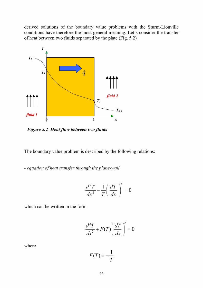
derived solutions of the boundary value problems with the Sturm-Liouville conditions have therefore the most general meaning. Let’s consider the transfer of heat between two fluids separated by the plate (Fig. 5.2) T T0 T1 fluid 2 T2 T0,0 fluid 1 0 1 x Figure 5.2 Heat flow between two fluids The boundary value problem is described by the following relations: - equation of heat transfer through the plane-wall

22

2

1 0d T dTdx T dx

⎛ ⎞− =⎜ ⎟⎝ ⎠

which can be written in the form

22

2 ( ) 0d T dTF Tdx dx

⎛ ⎞+ =⎜ ⎟⎝ ⎠

where

1( )F TT

= −

q&

47

the term 2

( )vk dTq xT dx⎛ ⎞= − ⎜ ⎟⎝ ⎠

&

represents the additional internal heat source. - the Sturm-Liouville boundary conditions x = 0 Heat transferred to the boundary surface x = 0.

fluid 1

h1

c o n v e c t io nq& 0xq

=&

T0 T1

x = 0

0convection xq q

==& &

which leads to the following condition:

( )1 0 10x

dTh T T kdx =

− = − (5.4)

where h1 is the coefficient of heat transfer from fluid 1 to the wall at x = 0.

48

x=1 Heat transferred from the boundary surface x = 1.

fluid 2 h2

1xq

=& c o n v e c t io nq&

T0,0 T2

x = 1

1 convectionxq q

==& &

which leads to the following condition:

( )2 2 0 ,01x

dTh T T kdx =

− = − (5.5)

where h2 is the coefficient of heat transfer from the plate to the fluid 2. In both boundary conditions, the values of h1, h2, k, T0 and T0,0 are known and the temperatures T1 and T2 are calculated. The solution to the boundary problem (5.4) and (5.5) describes the temperature field inside the plane-wall. In is important to mention that the boundary problem presented above is somewhat simplified where the entropy production at the near the wall at x=0 and x=1 has been assumed to be negligible. The full mathematical description would requires the introduction of two additional terms in the expression for entropy production: -for the near the wall surface at x=0

1

1 1

1

2

20

df f

f

k d Td x

d xT⎛ ⎞⎜ ⎟⎝ ⎠

∫

49

-for the near the wall surface at x=1

22 2

2

2

20

df f

f

k d Td x

d xT⎛ ⎞⎜ ⎟⎝ ⎠

∫

where

1fT and 2fT describe the temperature distribution, correspondingly in

the near the wall regions of fluid 1 (x=0) and fluid 2 (x= 1) with the thickness of d1 and d2 and heat conduction coefficients

1fk and

2fk . Since the thickness of the near the wall regions, in turbulent flows, is usually in the neighborhood of few millimeters, the influence of these additional entropy production can be ignored. The numerical analysis focuses therefore on the effect of the heat transfer coefficients h1 and h2 on the amount of entropy produced in the plate. The above discussion goes beyond the established aims of the thesis. However, the closer analysis demonstrates that including the convection (near the wall) terms of the entropy production would not be difficult from the methodological point of view and could be solved with the numerical methods. The simplified case of the problem discussed above has been presented by Rafois and Ortin [8]. 5.3 Boundary value problem with the simultaneous heat and electric current flow

The boundary value problem, generally non-linear, of the simultaneous heat and electric current flows with the boundary conditions of the first kind is being discussed here. The Joule’s heat is dissipated inside within the system. It is assumed that the heat conduction coefficient and the electric resistivity are functions of temperature, k=k(T) and ρ=ρ(T). The geometry of the system for the adiabatically insulated rod is shown in Figure 5.3.

50

adiabatically insulated rod surface T(x=0) = T1 T(x=1) = T2

inq& outq& x = 0 x = 1 Fig.5.3 Geometry of the adiabatically insulated rod surface Entropy generation rate is

2 2

2( ) ( )( )( ) ( )

k T dT i TxT x dx T x

ρσ ⎛ ⎞= +⎜ ⎟⎝ ⎠

where i is the electric current density Minimization

21 1 2

20 0

( ) ( )( ) minimum( ) ( )

k T dT i Tx dx dxT x dx T x

ρσ⎡ ⎤⎛ ⎞= + ⇒⎢ ⎥⎜ ⎟

⎝ ⎠⎢ ⎥⎣ ⎦∫ ∫

leads to Euler-Lagrange equation

22 2

21 ( ) 1 ( )( ) 0

2 ( ) 2 ( )d T dk T dT i d TT Tdx k T dT T dx k T dT

ρρ⎛ ⎞⎛ ⎞ ⎛ ⎞+ − + − =⎜ ⎟⎜ ⎟ ⎜ ⎟

⎝ ⎠ ⎝ ⎠⎝ ⎠

which can be written in the general form

22

1 22 ( ) ( ) 0d T d TF T F Td x d x

⎛ ⎞+ + =⎜ ⎟⎝ ⎠

additional internal heat source

k=k(T) ρ=ρ(T)

51

where

11 ( ) 1( )

2 ( )dk TF T

k T dT T= −

2

2( )( ) ( )

2 ( )i d TF T T T

k T dTρρ⎛ ⎞= −⎜ ⎟

⎝ ⎠

Boundary value problem is completed with the boundary conditions

1

2

( 0)( 1) .

T x TT x T

= == =

Several special cases have been analyzed by the use of various analytical and numerical methods. The work has been divided into four following situations:

k ρ

Case #1

k - constant

ρ - constant

Case #2

1

1

nTk kT

⎛ ⎞= ⎜ ⎟

⎝ ⎠

ρ - constant

Case #3

k-constant

11

nTT

ρ ρ⎛ ⎞

= ⎜ ⎟⎝ ⎠

Case#4

11

nTk kT⎛ ⎞

= ⎜ ⎟⎝ ⎠

oL Tk

ρ =

5.4 Methods of calculation of additional internal heat sources and entropy generation rate

The obtained solutions allow to determine the additional (resulting from the entropy production minimization) internal hear sources and the entropy generation rate. Particularly, the derivation of the Bernoulli equation from the Euler-Lagrange equation allows to derive these values. The difficulties that might be encountered during the calculations result from the non-explicit form of the solution.

52

1º - k=constant, boundary conditions of the first kind without the internal heat sources Boundary value problem is described by: - Euler-Lagrange equation

22

2

1 0d T dTdx T dx

⎛ ⎞− =⎜ ⎟⎝ ⎠

- boundary conditions

1

2

( 0)( 1) .

T x TT x T

= == =

where 2

( )( )vk dTq x

T x dx⎛ ⎞= − ⎜ ⎟⎝ ⎠

&

and the total heat source

21

,0

1( )( )v t

dTq x k dxT x dx

⎛ ⎞= − ⎜ ⎟⎝ ⎠∫&

Since

21

1

( )x

TT x TT

⎛ ⎞= ⎜ ⎟

⎝ ⎠

and

2 2 21

1 1 1

ln ( ) lnx

T T TdT T T xdx T T T

⎛ ⎞= =⎜ ⎟

⎝ ⎠

therefore

53

2

2

1

( ) ( ) lnvTq x kT xT

⎛ ⎞= − ⎜ ⎟

⎝ ⎠&

and

2; 1 2

1

( ) ln 0v tTq k T TT

= − <&

Entropy generation rate is

2

2 21

1 1

( )( ) ln( )

x

vq x T Tx kTT x T T

σ⎛ ⎞ ⎛ ⎞

= − = ⎜ ⎟ ⎜ ⎟⎝ ⎠ ⎝ ⎠

&

and

212

10

( ) ln 0( )

vt

q x Tdx kT x T

σ⎛ ⎞

= − = >⎜ ⎟⎝ ⎠

∫&

2º - k = k(T) , boundary conditions of the first kind without the internal heat sources Boundary value problem is described by: - Euler-Lagrange equation

22

21 ( )( ) 02

d T dk k T dTk Tdx dT T dx

⎛ ⎞⎛ ⎞+ − =⎜ ⎟⎜ ⎟⎝ ⎠⎝ ⎠ (5.6)

- boundary conditions

1

2

( 0)( 1) .

T x TT x T

= == = (5.7)

54

and 21 ( )( )

2vdk k T dTq xdT T dx

⎛ ⎞⎛ ⎞= − +⎜ ⎟⎜ ⎟⎝ ⎠⎝ ⎠

&

and the total amount of the heat source

21

,0

1 ( )2v t

dk k T dTq dxdT T dx

⎛ ⎞ ⎛ ⎞= − +⎜ ⎟ ⎜ ⎟⎝ ⎠ ⎝ ⎠∫&

and entropy generation rate connected with heat source becomes

21 1 ( )( )( ) 2

dk k T dTxT x dT T dx

σ ⎛ ⎞ ⎛ ⎞= +⎜ ⎟ ⎜ ⎟⎝ ⎠ ⎝ ⎠

and

21

0

1 1 ( )( ) 2t

dk k T dT dxT x dT T dx

σ ⎛ ⎞⎛ ⎞= +⎜ ⎟⎜ ⎟⎝ ⎠⎝ ⎠∫

The functional relations for T(x) and dT/dx are determined by solutions to equations (5.6) and (5.7) after prior calculation of the integration constants, while F2(T) = 0. The total entropy production is

( )

21

20

( )( )

tk T dT dx

dxT xσ ⎛ ⎞= ⎜ ⎟

⎝ ⎠∫

or

( )

2

1

2( )( )

T

tT

k T dT dTdxT x

σ = ∫

Solution to Eq.(5.6) can be easily obtained by the substitution

55

dT udx

=

which gives

2

2d T du udx dT

=

and equation (5.6) takes the form

( ) ( ) 0duk T F T udT

+ =

(5.8) where

1 ( )( )2

dk k TF TdT T

= −

The solution of (5.8) is

( )( )

1

F T dTk TdTu c e

dx

−∫= =

which after simplification gives

1 ln ( ) ln2

1

k T TdT c edx

+=

hence

1 ( )dT c T k Tdx

=

and

1 1 2( )( )

dT c dx c x cTk T

= = +∫ ∫

Finally

56

[ ]2

1

32( )T

tT

k TdT

Tσ = ∫

3° - k=constant, boundary conditions of the third kind (Sturm-Liouville boundary conditions) without the internal heat sources. Boundary value problem is described by: - Euler-Lagrange equation

22

2

1 0d T dTdx T dx

⎛ ⎞− =⎜ ⎟⎝ ⎠ (5.9)

- boundary conditions

1 0 00

2 0,011

0 ( )

1 ( )

xx

xx

dTfor x k h T TdxdTfor x k h T Tdx

==

==

= − = −

= − = −

(5.10) The general solution has the form

13( ) c xT x c e=

hence (5.11)

13 1

c xdT c c edx

=

Substitution of expressions (5.11) into the boundary conditions (5.10) gives

57

1 1

1 3 1 3 1

1 3 2 3 2c c

kc c h c

kc c e h c e

γ

γ

− + =

− − =

(5.12) where

1 1 0 2 2 0,0andh T h Tγ γ= = − The values of c1 and c3 are numerically determined because of the non-explicit character of equations (5.12). The additional internal heat source is

2

( )( )vk dTq x

T x dx⎛ ⎞= − ⎜ ⎟⎝ ⎠

&

and its total value is

21

,0

1( )( )v t

dTq x k dxT x dx

⎛ ⎞= − ⎜ ⎟⎝ ⎠∫&

Using equations (5.10) leads to

123 1( ) c x

vq x kc c e= −& and

1, 1 3( ) (1 )c

v tq x kc c e= −& Entropy generation rate is

21

( )( ) 0( )

vq xx kcT x

σ = = >&

and is equal to σt as div s&= 0.

58

4° - k = k(T), boundary conditions of the third kind (Sturm-Liouville boundary conditions) without the internal heat sources. Boundary value problem is described by: - Euler-Lagrange equation

22

21 1 0

2d T dk dTdx k dT T dx

⎛ ⎞ ⎛ ⎞+ − =⎜ ⎟ ⎜ ⎟⎝ ⎠ ⎝ ⎠

(5.13)

- boundary conditions

1 00 00

2 0,01 11

0 ( ) ( )

1 ( ) ( )

x xx

x xx

dTfor x k T h T TdxdTfor x k T h T Tdx

= ==

= ==

= − = −

= − = −

(5.14)

After substitution u=dT/dx, equation (5.13) becomes

( ) 0du F T udT

+ =

while

1 1( )2

dkF Tk dT T

= −

which leads to equation

( )1

F T dTdTu c edx

−∫= =

(5.15)

59

and after the second integration

2( )1

F T dT

dT x cc e−

= +∫∫

(5.16) Equation (5.16) is given in the non-explicit form. The additional internal heat source is given by:

21 ( )( )2v

dk k T dTq xdT T dx

⎛ ⎞⎛ ⎞= − +⎜ ⎟⎜ ⎟⎝ ⎠⎝ ⎠

&

and

21

,0

1 ( )( )2v t

dk k T dTq x dxdT T dx

⎛ ⎞⎛ ⎞= − +⎜ ⎟⎜ ⎟⎝ ⎠⎝ ⎠∫&

while T(x) and dT/dx are described by equations (5.13) and (5.14). Examples of the numerical analysis are provided in Chapter 7. Entropy production at the additional heat source takes the form

2( ) 1 1 ( )( )

( ) ( ) 2vq x dk k T dTx

T x T x dT T dxσ ⎛ ⎞ ⎛ ⎞= − = +⎜ ⎟ ⎜ ⎟

⎝ ⎠ ⎝ ⎠

&

and

21

0

1 1 ( )( ) 2t

dk k T dT dxT x dT T dx

σ ⎛ ⎞⎛ ⎞= − +⎜ ⎟⎜ ⎟⎝ ⎠⎝ ⎠∫

Total value of the entropy production comes from the definition

60

2

1

21

2 20

( ) ( )T

tT

k T dT k T dTdx dTT dx T dx

σ ⎛ ⎞= =⎜ ⎟⎝ ⎠∫ ∫

and is obtained in the same way as in 2º. 5º - Simultaneous heat and electric current flows, k = k(T) , ρ = ρ(T) Boundary value problem is described by: - Euler-Lagrange equation

22

1 22 ( ) ( ) 0d T d TF T F Td x d x

⎛ ⎞+ + =⎜ ⎟⎝ ⎠

(5.17) where

11 ( ) 1( )

2 ( )dk TF T

k T dT T= −

2

2( )( ) ( )

2 ( )i d TF T T T

k T dTρρ⎛ ⎞= −⎜ ⎟

⎝ ⎠

- boundary conditions

1

2

( 0 )( 1)

T x TT x T

= == =

(5.18)

It can be easily shown that equation (5.17) can be transformed into the Bernoulli equation in the form

11 2( ) ( )du F T u F T u

dT−+ = −

(5.19)

61

where d Tud x

=

The additional internal heat source is

2 21 ( )2 2v

dk k T dT i dq TdT T dx dT

ρρ⎛ ⎞⎛ ⎞ ⎛ ⎞= − + − +⎜ ⎟⎜ ⎟ ⎜ ⎟⎝ ⎠⎝ ⎠ ⎝ ⎠

&

and

1

,0

( )v t vq q x dx= ∫& &

In general, because of the non-explicit form of the solution, the numerical calculations must follow. Energy generation rate at the additional heat source is

2 2( ) 1 1 ( ) ( )( ) ( )( ) ( ) 2 2

vq x dk T k T dT i dx T TT x T x dT T dx dT

ρσ ρ⎡ ⎤⎛ ⎞⎛ ⎞ ⎛ ⎞= − = + + +⎢ ⎥⎜ ⎟⎜ ⎟ ⎜ ⎟⎝ ⎠⎝ ⎠ ⎝ ⎠⎢ ⎥⎣ ⎦

&

and

21 2

0

1 1 ( ) ( ) ( )( ) 2 2t

dk T k T dT i dT T dxT x dT T dx dT

ρσ ρ⎡ ⎤⎛ ⎞⎛ ⎞ ⎛ ⎞= + + +⎢ ⎥⎜ ⎟⎜ ⎟ ⎜ ⎟⎝ ⎠⎝ ⎠ ⎝ ⎠⎢ ⎥⎣ ⎦

∫

Total value of the entropy production comes from definition

2 2

1 1

12

2( )T T

tT T

k T dT i dTdT dTT dx T dx

ρσ−

⎛ ⎞= + ⎜ ⎟⎝ ⎠∫ ∫

where T(x) and dT/dx are obtained from the solution of Bernoulii equation (5.19) (see next Chapter 6).

62

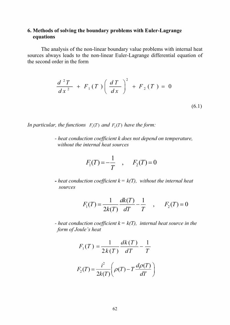
6. Methods of solving the boundary problems with Euler-Lagrange equations

The analysis of the non-linear boundary value problems with internal heat sources always leads to the non-linear Euler-Lagrange differential equation of the second order in the form

22

1 22 ( ) ( ) 0d T d TF T F Td x d x

⎛ ⎞+ + =⎜ ⎟⎝ ⎠

(6.1)

In particular, the functions 1 ( )F T and 2 ( )F T have the form:

- heat conduction coefficient k does not depend on temperature, without the internal heat sources

1 21( ) , ( ) 0F T F TT

= − =

- heat conduction coefficient k = k(T), without the internal heat sources

1 21 ( ) 1( ) , ( ) 0

2 ( )dk TF T F T

k T dT T= − =

- heat conduction coefficient k = k(T), internal heat source in the form of Joule’s heat

11 ( ) 1( )

2 ( )dk TF T

k T dT T= −

2

2( )( ) ( )

2 ( )i d TF T T T

k T dTρρ⎛ ⎞= −⎜ ⎟

⎝ ⎠

63

The specific form (6.1) of the Euler-Lagrange equations, when F1(T) and F2(T) are both not equal to zero, allows to obtain an analytical solution, usually though in the non-explicit form.

By substitution dT udx

=

and differentiating

2

2

d T du du dT du udx dx dT dx dT

= = =

after substituting into (5.19) gives

2

1 2( ) ( ) 0du u F T u F TdT

+ + =

Finally equation (5.19) becomes

11 2( ) ( )du F T u F T u

dT−+ = − (6.2)

Equation (6.2) represents the Bernoulli differential equation which has the general solution in the non-explicit form:

1 1

22 ( ) 2 ( )

2 12 ( )F T dT F T dTdT e F T e cdx

⎛ ⎞ ∫ ∫= − +⎜ ⎟⎝ ⎠ ∫

(6.3) Hence

1 1

122 ( ) 2 ( )

2 12 ( ) F T dT F T dTdT F T e c edx

−⎧ ⎫⎡ ⎤∫ ∫= − +⎨ ⎬⎢ ⎥⎣ ⎦⎩ ⎭∫

(6.4)

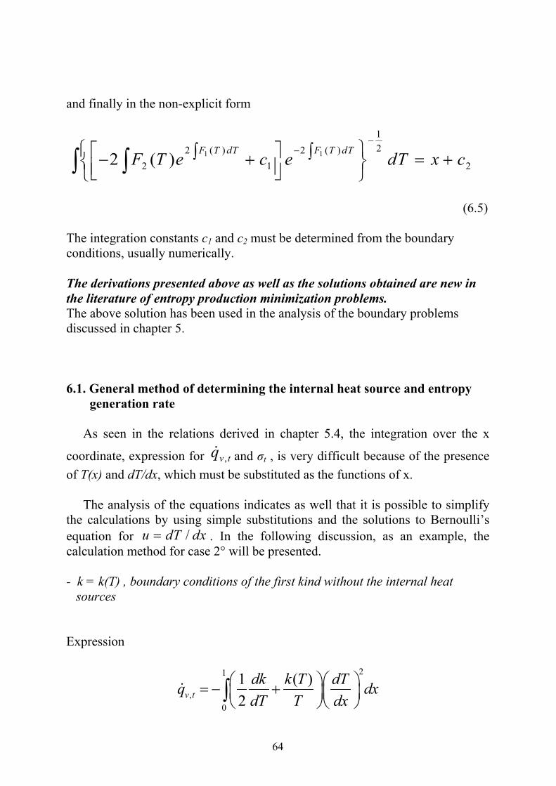
64

and finally in the non-explicit form

1 1

122 ( ) 2 ( )

2 1 22 ( ) F T dT F T dTF T e c e dT x c−

−⎧ ⎫⎡ ⎤∫ ∫− + = +⎨ ⎬⎢ ⎥⎣ ⎦⎩ ⎭∫ ∫

(6.5) The integration constants c1 and c2 must be determined from the boundary conditions, usually numerically. The derivations presented above as well as the solutions obtained are new in the literature of entropy production minimization problems. The above solution has been used in the analysis of the boundary problems discussed in chapter 5. 6.1. General method of determining the internal heat source and entropy

generation rate

As seen in the relations derived in chapter 5.4, the integration over the x

coordinate, expression for ,v tq& and σt , is very difficult because of the presence of T(x) and dT/dx, which must be substituted as the functions of x.

The analysis of the equations indicates as well that it is possible to simplify

the calculations by using simple substitutions and the solutions to Bernoulli’s equation for /u dT dx= . In the following discussion, as an example, the calculation method for case 2° will be presented. - k = k(T) , boundary conditions of the first kind without the internal heat sources Expression

21

,0

1 ( )2v t

dk k T dTq dxdT T dx

⎛ ⎞⎛ ⎞= − +⎜ ⎟⎜ ⎟⎝ ⎠⎝ ⎠∫&

65

can be rewritten in the form

1

,0

1 ( )2v t

dk k T dT dTq dxdT T dx dx

⎛ ⎞= − +⎜ ⎟⎝ ⎠∫&

hence

2

1

,1 ( )2

T

v tT

dk k T dTq dTdT T dx

⎛ ⎞= − +⎜ ⎟⎝ ⎠∫&

(6.6) By substitution

( )dTu Tdx

= = Φ

(6.7) the integration of (6.6) becomes much easier, as dT/dx is the indirect function of x (as T=T(x)). Substituting (6.7) into (6.6) yields

2

1

,1 ( ) ( )2

T

v tT

dk k Tq T dTdT T

⎛ ⎞= − + Φ⎜ ⎟⎝ ⎠∫&

In the identical way, the calculation for the entropy production resulting from the additional heat source can be simplified by transforming expression

21 1

0 0

1 1 ( )( ) ( ) 2

vt

q dk k T dTdx dxT x T x dT T dx

σ ⎛ ⎞⎛ ⎞= − = +⎜ ⎟⎜ ⎟⎝ ⎠⎝ ⎠∫ ∫

&

into

2

1

1 1 ( )( ) 2

T

tT

dk k T dT dTT x dT T dx

σ ⎛ ⎞= +⎜ ⎟⎝ ⎠∫

66

using, as before,

( )dTu Tdx

= = Φ

The calculations can be done in the same way as for other boundary problems without the internal heat sources. Total value of the entropy production comes from definition

2

1

2( )T

tT

k T d T d TT d x

σ = ∫

(6.8) and the solution is identical as in 2º. For the problem of simultaneous heat and electric current flows, the above analysis requires modification. Entropy production describing additional heat source becomes

21 2

0

1 1 1 ( )( ) 2 ( ) 2 ( )t

dk dT i dT T dxT x k T dT T dx k T dT

ρσ ρ⎡ ⎤⎛ ⎞⎛ ⎞ ⎛ ⎞= + + +⎢ ⎥⎜ ⎟⎜ ⎟ ⎜ ⎟

⎝ ⎠ ⎝ ⎠⎝ ⎠⎢ ⎥⎣ ⎦∫

which can be written in the form of two integrals

2

1

112

0

1 1 1( ) 2 ( )

1 ( )2

T

tT

dk dT dTT x k T dT T dx

d dTi T T dTdT dx

σ

ρρ−

⎡ ⎤⎛ ⎞= +⎢ ⎥⎜ ⎟

⎝ ⎠⎣ ⎦

⎡ ⎤⎛ ⎞⎛ ⎞+ +⎢ ⎥⎜ ⎟⎜ ⎟⎝ ⎠⎝ ⎠⎢ ⎥⎣ ⎦

∫

∫

Transformation above allows, as before, for solving the Bernoulli equation for

67

( )dTu Tdx

= = Φ

which after substituting into expression for σt leads to the direct expression

2 2

1 1

12

2( )T T

tT T

k T dT i dTdT dTT dx T dx

ρσ−

⎛ ⎞= + ⎜ ⎟⎝ ⎠∫ ∫

The method described above is the new concept in literature dealing with entropy production minimization, calculation of the internal heat sources and entropy production σt . The most important feature of this method is that it can be applied to any mathematical relationship for k=k(T) and ρ=ρ(T) as the solution of the governing differential equation is given in the general form.

68

7. Solutions for the specific boundary value problems 7.1 Simultaneous heat and electric current flows

All the calculations below originate from the general solution (6.4) which can be easily rearranged into

1

1

2 ( )22

2 ( )

2 ( ( ) F T dT

F T dT

F T e dTdTdx e

∫−⎛ ⎞ =⎜ ⎟ ∫⎝ ⎠∫

(7.1)

Case#1 The values for k, ρ are both constant General equation

( ) 02

'121''

22 =⎟

⎠⎞

⎜⎝⎛ −+⎟

⎠⎞

⎜⎝⎛ −+

dTdT

kiT

TdTdk

kT ρρ

is simplified to the form

( )21'' ' 0T TT

α− + =

(7.2) where

2

2'' d TTdx

=

' dTTdx

=

2

2i

kρα =

69

which according to (7.1) has the solution for F1(T)= - 1/T and F2(T)= α in the form:

( )12

22 2

1122

12 ( )( )221

dTT

dTT

dTe dTdT T T c Tdx

e T

ααα

⎛ ⎞−⎜ ⎟⎝ ⎠

⎛ ⎞−⎜ ⎟⎝ ⎠

∫ −−⎛ ⎞ ⎡ ⎤= = = −⎜ ⎟ ⎣ ⎦⎝ ⎠ ∫

∫∫

(7.3) Hence

21

2dT dxT c T

α=−

∫ ∫

(7.4) which after the substitution

11

12

w c Tc

= −

gives

21

2

1

1 21

2

dw dxc

wc

α− =⎛ ⎞

−⎜ ⎟⎜ ⎟⎝ ⎠

∫ ∫

after integration

11 2

1

1 sin (1 2 ) 2 ( )c T x cc

α−− − = +

an explicit solution becomes

1 2

1

1 sin 2 ( )( )

2

c x cT x

c

α⎡ ⎤+ +⎣ ⎦=

(7.5)

70

Applying boundary conditions, two algebraic equations are obtained which allow to find the integration constants c1 and c2

1 1 1 21 2 sin 2 ( )c T c cα⎡ ⎤− = −⎣ ⎦ and

1 2 1 21 2 sin 2 (1 )c T c cα⎡ ⎤− = − +⎣ ⎦ The graphs of T (x) vs. x are shown in Fig. 7.1.

Fig. 7.1 The graph of T(x) vs. x for different values of boundary temperatures when k=constant and ρ=constant Local entropy production σ(x) can also be calculated according to

2 2

2( )( ) ( )k dT ix

T x dx T xρσ ⎛ ⎞= +⎜ ⎟

⎝ ⎠

71

it is assumed that 2

= 12i K

kρα =

Therefore

[ ]

212

4 2( )( )( )

k T c T kxT xT x

α ασ⎡ ⎤−⎣ ⎦= +

and

14( ) 2

( )kx kc

T xασ α= −

The graph of local entropy production σ(x) vs. x is shown in Fig. 7.2.

Fig. 7.2 The graph of local entropy production σ(x) vs. x for different values of boundary temperatures when k=constant and ρ=constant

72

The total entropy production σt can also be calculated according to:

1 1

10 0

2( ) 2( )t x dx k c

T xσ σ α

⎡ ⎤= = −⎢ ⎥

⎣ ⎦∫ ∫

Assuming k = 20 W/mK , the following numerical values for total entropy production are obtained and shown in Table 7.1. Table 7.1

Boundary Temperatures

T1=0.4 T2=0.1

T1=0.8 T2=0.5

T1=1.0 T2=0.6

T1=1.0 T2=0.7

Total Entropy

Production σt

(W/K)

226.4

63.6

54.8

48.4

The internal heat source

2 21( )2 2v

dk k dT i dq x TdT T dx dT

ρρ⎛ ⎞⎛ ⎞ ⎛ ⎞= − + − +⎜ ⎟⎜ ⎟ ⎜ ⎟⎝ ⎠⎝ ⎠ ⎝ ⎠

&

can also be calculated and when k=constant and ρ=constant:

2 2

( )2v

k dT iq xT dx

ρ⎛ ⎞= − −⎜ ⎟⎝ ⎠

&

substituting for (dT/dx)2 from Eq. 7.3 gives

22

1 1( ) 2 ( 3 22v

k iq x T cT k kcTT

ρα α α⎡ ⎤= − − − = − +⎣ ⎦&

and

73

1 2( ) 3 1 sin 2 ( )vq x k k c x cα α α⎡ ⎤⎡ ⎤= − + + +⎣ ⎦⎣ ⎦&

Finally

{ }1 1

, 1 20 0

( ) 2 sin 2 ( )v t vq q x dx k c x c dxα α⎡ ⎤= = − + +⎣ ⎦∫ ∫& &

Assuming again k = 20 W/mK , the following numerical values for the total heat source are calculated and presented in Table 7.2. Table 7.2

Boundary Temperatures

T1=0.4 T2=0.1

T1=0.8 T2=0.5

T1=1.0 T2=0.6

T1=1.0 T2=0.7

Total Heat Source

,v tq& (W)

-31

-24.6

-25.4

-24.2

Case #2 Conditions:

n

TTkk ⎟⎟

⎠

⎞⎜⎜⎝

⎛=

11 and ρ = constant

General equation

( ) 02

'121''

22 =⎟

⎠⎞

⎜⎝⎛ −+⎟

⎠⎞

⎜⎝⎛ −+

dTdT

kiT

TdTdk

kT ρρ

becomes

74

22 1'' ( ') 02 n

nT TT T

α−+ + =

(7.6) where

21

12

ni Tk

ρα =

which according to equation (7.1) has the solution for

12 1( )

2nF T

T−

=

and

2 ( ) nF TTα−=

in the form:

2 122 22

12 12 12

2

2 2 2 (1 )

n dTT n

n n

n nn dTT

e dT T dTdT c TT Tdx T T

e

α αα

−⎛ ⎞⎜ ⎟⎝ ⎠ −

− −−⎛ ⎞⎜ ⎟⎝ ⎠

− ∫⎛ ⎞ −⎜ ⎟ −⎛ ⎞ ⎝ ⎠= = =⎜ ⎟

⎝ ⎠ ∫

∫ ∫

(7.7) Hence

12

1

21

n

T dT dxc T

α

−

=−∫ ∫

(7.8)

75

Table 7.3 below is the summary of the integrals obtained and the solutions for different values of n. Table 7.3 n integral solution

-2 21

2( )

dT dxT T c T

α=−

∫ ∫

2

12

22 ( )

T c Tx c

Tα

− −= +

-1

1

21dT dx

T c Tα=

−∫ ∫ 12

1

1 1ln 2 ( )

1 1c T

x cc T

α− −

= +− +

0

21

2dT dxT c T

α=−

∫ ∫ 1 2

1

1 sin 2 ( )( )

2

c x cT x

c

α⎡ ⎤+ +⎣ ⎦=

Same as in case#1, k, ρ constant 1

1

21

dT dxc T

α=−∫ ∫ 1

21

2 12 ( )

c Tx c

cα

−= +

−

k-linear, ρ - constant 2 1 / 2

1

21

T dT dxc T

α=−∫ ∫

1

1 123/2

1 1

sin ( ) 12 ( )

cT T cTx c

c cα

− −− = +

3

1

21T dT dx

c Tα=

−∫ ∫

( )11 22

1

2 21 2 ( )

3cT

cT x cc

α+

− − = +

76

The total entropy production can be determined with the described earlier

2 2

1 1

21 1 2

20 0

2

2

( ) ( )

( ) ( ) 1

t

T T

T T

k T dT i Tdx dxT dx T

k T dT i TdT dTdTT dx Tdx

ρσ

ρ

⎛ ⎞= + =⎜ ⎟⎝ ⎠

⎛ ⎞= +⎜ ⎟ ⎛ ⎞⎝ ⎠⎜ ⎟⎝ ⎠

∫ ∫

∫ ∫

(7.9) Applying this method in Case#2 yields

2 2

1 1

2 2

1 1

1 1 21

12 12

12

33 2 2

1 21

1 1

2 (11

2 (1 )

2 12 1

n

T T

t nT T

n

nT Tn

nT T

Tk c TT i dT

T c TT TT

k i TT c T dT dTT c T

αρσ

α

α ρα

−

−

−−

⎛ ⎞−⎜ ⎟

⎝ ⎠= + =−

= − +−

∫ ∫

∫ ∫

which provides a general expression which can be calculated numerically for the specific boundary conditions.

77

In the section below, a specific solution for n=1 (k-linear function of temperature, ρ – constant, same as Case#4) is examined. Solution

12

1

2 12 ( )

c Tx c

cα

−= +

−

results in

2 21 2

1

11 ( )2( )

c x cT x

c

α− +=

(7.10) or

2 21 1 2 1 2

1

1 1 1( )2 2

T x c x c c x c cc

α α α= − − + −

which produces the following graphs for the specific boundary temperatures, represented in Fig.7.1.

Fig. 7.3 Graph of T(x) versus x for n=1 and for different values of boundary temperatures when k=linear and ρ=constant

78

The local entropy production can be calculated according to:

2 2

2( )( )( ) ( )

k T dT ixT x dx T x

ρσ ⎛ ⎞= +⎜ ⎟⎝ ⎠

which in this case becomes

( )1

21 11

1 121 1

2 1 2 1( ) 2 1

k Ti k kTx c T c

T T T T T Tρ α ασ α ⎛ ⎞= − + = − +⎜ ⎟

⎝ ⎠

as

221

1

12

ni T Kkρ

α = =

and

T1=1 (dimensionless temperature) the following expression is obtained:

11

1

2 2( )( )

kx cT T xασ

⎛ ⎞= −⎜ ⎟

⎝ ⎠

which is represented graphically in Fig 7.2.

79

Fig.7.4 Graph of local entropy production σ(x) versus x for n=1 and for different values of boundary temperatures when k=linear and ρ=constant The total entropy production σt can also be calculated according to:

1 11

110 0

2 2( )( )t

kx dx c dxT T xασ σ

⎛ ⎞= = −⎜ ⎟

⎝ ⎠∫ ∫

Assuming k1 = 20 W/mK , the following numerical values for total entropy production are obtained and shown in Table 7.4.

Table 7.4 Boundary

Temperatures T1=1.0 T2=0.1

T1=1.0 T2=0.3

Total Entropy

Production σt

(W/K)

139.2

82

80

The internal heat source

2 21 ( )( )2 2v

dk k T dT i dq x TdT T dx dT

ρρ⎛ ⎞⎛ ⎞ ⎛ ⎞= − + − +⎜ ⎟⎜ ⎟ ⎜ ⎟⎝ ⎠⎝ ⎠ ⎝ ⎠

&

can also be calculated, giving

[ ]2

1 11

1 1

1( ) 2 (12 2v

k k iq x cTT T

ρα⎛ ⎞

=− + − −⎜ ⎟⎝ ⎠

&

or

[ ]1 11

1 1

3( ) 1vk kq x cT

T Tα α

= − − −&

and finally

2 211 2

1

3( ) 1 ( ) 02v

kq x c x cTα α⎡ ⎤= − + + <⎢ ⎥⎣ ⎦

&

therefore

1 12 21

, 1 210 0

3( ) 1 ( )2v t v

kq q x dx c x c dxTα α⎡ ⎤= =− + +⎢ ⎥⎣ ⎦∫ ∫& &

Assuming k1 = 20 W/mK , the following numerical values for the total heat source are calculated and presented in Table 7.5. Table 7.5

Boundary Temperatures

T1=1.0 T2=0.1

T1=1.0 T2=0.3

Total Heat Source

,v tq& (W)

-46.4

-37.0

81

Case#3 Conditions:

k= constant and n

TT⎟⎟⎠

⎞⎜⎜⎝

⎛=

11ρρ

General equation

( ) 02

'121''

22 =⎟

⎠⎞

⎜⎝⎛ −+⎟

⎠⎞

⎜⎝⎛ −+

dTdT

kiT

TdTdk

kT ρρ

becomes

21'' ( ') ( ) 0T T g TT

− + =

(7.11) where

21

1

( ) (1 )2

nn

ig T n T andkTρα α= − =

which according to (7.1) has the solution for

11( )F TT

= −

and

2 ( ) (1 ) nF T n Tα= − in the form:

82

122ln2

2ln12

22

2 2

1

12 1

1

2

2 ( (1 ) 2 ( (1 )

12 ( (1 ) 2 ( 1)1 1

2 ( 1)1

2 ( 1)1

dTn n TT

TdT

T

n n

n

n

n T e n T edTdx e

e

n T dT n T dTT

T TTn cn

T T n c

T

α α

α α

αα

⎛ ⎞−⎜ ⎟ −⎝ ⎠

−⎛ ⎞−⎜ ⎟⎝ ⎠

−

−

−

∫− − − −⎛ ⎞ = = =⎜ ⎟

⎝ ⎠ ∫

− − −= = =

⎡ ⎤− +⎢ ⎥−⎣ ⎦ ⎡ ⎤= = + −⎣ ⎦

∫ ∫

∫ ∫

Hence:

11( 1)n

dTT T n c−

=+ −∫

1 21

2( 1)n

dT dxT n c T

α+

= =+ −

∫ ∫

(7.12) Note: In case of n=1 (k-constant, ρ –linear), the above integral solution can not be used as F2 = 0 and equation

21'' ( ') ( ) 0T T g TT

− + =

becomes 21'' ( ') 0T T

T− =

the substitution u=dT/dx leads to the known solution

21

1

xTT TT

⎛ ⎞= ⎜ ⎟

⎝ ⎠

83

Table 7.6 is the summary of the integrals obtained and the solutions for different values of n. Table 7.6

n integral solution

-2

31

21 3

T dT dxc T

α=−

∫ ∫

1 3 / 2

12

1

2 sin ( 3 )2 ( )

3 3c T

x cc

α−

= +

-1

21

21 2

dT dxcT

α=−

∫ ∫

( )11 2

1

1 sin 2 2 ( )2

cT x cc

α− = +

0

21

2dT dxT cT

α=−

∫ ∫ 1 2

1

1 sin 2 ( )( )

2

c x cT x

c

α⎡ ⎤+ +⎣ ⎦=

same as in Case#1, k,ρ constant 2

1

2dT dxT T c

α=+∫ ∫

12

1ln 2 ( )

1T c

x cT c

α+ −

= ++ +

3

21

22

dT dxT T c

α=+

∫ ∫

2

1 12

1

2 21 ln 2 ( )2

c T cx c

Tcα

⎛ ⎞+ +⎜ ⎟− = +⎜ ⎟⎝ ⎠

84

The total entropy can be determined with the use of the method described in Case#2 (equation 7.7)

2 2

1 1

2 2

1 1

211

1 1 12 1

1

1 2 21 1

1 11 1

2 ( 1) 1( 1)

( 1)2

2 ( 1)

n

T Tn

t nT T

T Tn n

n nT T

TikT T n c T

dT dTT T T T n c

T n c i Tk dT dTT T T n c

ρα

σ

ραα

−

−

− −

−

⎛ ⎞⎜ ⎟+ − ⎝ ⎠= +

+ −

+ −= +

+ −

∫ ∫

∫ ∫ Case #4 Conditions:

n

TTkk ⎟⎟⎠

⎞⎜⎜⎝

⎛=

11 , k

TL0=ρ (Wiedemann-Franz Law)

General equation

( ) 02

'121''

22 =⎟

⎠⎞

⎜⎝⎛ −+⎟

⎠⎞

⎜⎝⎛ −+

dTdT

kiT

TdTdk

kT ρρ

becomes

22 1'' ( ') ( ) 02

nT T g TT

−+ + =

(7.13) where

1

2 21 2 0 1

2( )2

nn i L Tg T n T and

kα α−= =

which according to (7.1) has the solution for

12 1( )

2nF T

T−

=

and

85

1 22 ( ) nF T n Tα −=

in the form:

( 2) 121 2 1 2 ( 2) ln2 2

( 2) 1 ( 2) ln22

1 2 2 1 1

2 2 2

1 12 2 2

2 ( 2 (

22 ( 2 (

2 2 1

n dTn n n TT

n n TdTT

n

n n n

n n n

n n

n n

n T e dT n T e dTdTdx e

eTn cn T T dT n T dT n

T T TT nc ncTT T

α α

αα α

α α

−− − −

− −

−

− − − −

− − −

−

− −

∫− −⎛ ⎞ = = =⎜ ⎟⎝ ⎠ ∫

⎡ ⎤− +⎢ ⎥− − −⎣ ⎦= = = =

⎡ ⎤ ⎡ ⎤− −⎣ ⎦ ⎣ ⎦= =

∫ ∫

∫ ∫

Hence:

1

1

21

n

n

T dT dxnc T

α−

=−

∫ ∫

(7.14) Note: In case of n=0 (k-constant, ρ –linear), the above integral solution can not be used as F2 = 0 and equation

21'' ( ') ( ) 0T T g TT

− + =

becomes 21'' ( ') 0T T

T− =

the substitution u=dT/dx leads to the known solution

21

1

xTT TT

⎛ ⎞= ⎜ ⎟

⎝ ⎠

86

Table 7.7 is the summary of the integrals obtained and the solutions for different values of n. Table 7.7 n integral solution 1

1

21dT dx

cTα=

−∫ ∫

12

1

2 12 ( )

c Tx c

cα

−= +

−

same as in case #2 (for n=1) k-linear, ρ-constant 2

21

21 2

TdT dxc T

α=−

∫ ∫

22

11

1 1 2 ( )22

T x ccc

α− − = +

3

2

31

21 3

T dT dxc T

α=−

∫ ∫

31 2

1

2 1 3 2 ( )9

c T x cc

α− − = +

The total entropy production can be determined with the use of the method described in Case#2

2 2

1 1

2 2

1 1

1 1 21 0

2 11

1 11

21 0 11

1 1 1

2 (1 )1

2 (1 )

122 1

nn

T T

t nn nT T

n

T Tn n

n nT T

Tk nc TT i L TdT dT

T T nc TTT kT T

nc T i L Tk dTdTT T k T nc T

ασ

α

αα

−

−

⎛ ⎞−⎜ ⎟

⎝ ⎠= + =−⎛ ⎞

⎜ ⎟⎝ ⎠

−= +

−

∫ ∫

∫ ∫

87

7.2 Boundary conditions of the second and third kinds - heat conduction coefficient independent of temperature

Case#1 – Boundary conditions of the second kind (gradient at x=0)

22

21 0d T dT

dx T dx⎛ ⎞− =⎜ ⎟⎝ ⎠

2

0 constant

1 (1)

dTxdx

x T T

β= = =

= =

the solution is 1

3( ) c xT x c e= The graph of T(x) vs. x for dT/dx = -1 and different values of T2 is shown in Fig. 7.5.

Fig.7.5 Graph of T(x) versus x for dT/dx = -1 and for different values of T2 .

88

Local entropy production

( )1

1

22 2

3 1 1 t22

3

( ) constant = ( )

c x

c x

k dT kx c c e kcT x dx c e

σ σ⎛ ⎞= = = =⎜ ⎟⎝ ⎠ ⎡ ⎤⎣ ⎦

Assuming, as before k = 20 W/mK , the following numerical values for total entropy production are obtained and shown in Table 7.8. Table 7.8

Boundary value at x=1

T2=0.1 T2=0.2 T2=0.5 T2=0.8 T2=1.0

Total Entropy Production

σt (W/K)

60.9

35.2

14.5

8.5

6.4

Case#2 - Boundary conditions of the second kind (gradient at x = 1)

22

2

1 0d T dTT dxdx⎛ ⎞− =⎜ ⎟⎝ ⎠

1

1

0 ( 0)

1

x T x TdTxdx

β

= = =

= =

the solution is 1

3( ) c xT x c e= The graph of T(x) vs. x for different values of β1 and for T1=1.0 is shown in Fig. 7.6. In addition, local entropy production

( )1

1

22 2

3 1 1 t22

3

( ) constant = ( )

c x

c x

k dT kx c c e kcT x dx c e

σ σ⎛ ⎞= = = =⎜ ⎟⎝ ⎠ ⎡ ⎤⎣ ⎦

89

Fig.7.6 Graph of T(x) versus x for different values of dT/dx and for T1=1.0 Case#3 - Boundary conditions of the third kind (Sturm-Liouville boundary conditions).

22

21 0d T dT

dx T dx⎛ ⎞− =⎜ ⎟⎝ ⎠

0 1 0 0

1 2 1 0,0

0 ( )

1 ( )

x x

x x

dTx k h T TdxdTx k h T Tdk

= =

= =

= − = −

= − = −

or

0 1 0 1 0 1

1 2 1 2 0,0 2

x x

x x

dTk h T hTdxdTk h T h Tdk

γ

γ

= =

= =

− + = =

− − = − =

90

which in combination with the solution

xcecxT 1

3)( = results in the following equation for constant c1:

1

1 2

1 1 1 2( )ch kc e kc hγ γ−

=− +

where

13

1 1

ch k c

γ=

−

Taking T0=1.3 , T0,0=0.85 (dimensionless temperatures)

h1=h2=20, 200, 2000 W/m2K k = 20 W/mK γ1= h1T0 = 26, 260, 2600 W/m2K γ2= -h2T0,0 = -17, -170, -1700 W/m2K

results in the following graph of T(x) vs. x as shown in Fig.7.7.

Fig.7.7 Graph of T(x) vs. x for different values of heat transfer coefficient h and for T0,0=0.85

91

Similarly, taking T0=1.3 , T0,0=0.05

h1=h2=20, 200, 2000 W/m2K k = 20 W/mK γ1= h1T0 = 26, 260, 2600 W/m2K γ2= -h2T0,0 = -1, -10, -100 W/m2K

the graphs presented in Fig. 7.8 are produced.

Fig.7.8 Graph of T(x) vs. x for different values of heat transfer coefficient h and for T0,0=0.05 Local entropy production, as in the previous cases is given by

( )1

1

22 2

3 1 1 t22

3

( ) constant = ( )

c x

c x

k dT kx c c e kcT x dx c e

σ σ⎛ ⎞= = = =⎜ ⎟⎝ ⎠ ⎡ ⎤⎣ ⎦

92

7.3 Boundary conditions of the third kind (Sturm-Liouville boundary conditions) - heat conduction coefficient dependent on temperature

( )21 1'' ' 02

dkT Tk dT T

⎛ ⎞+ − =⎜ ⎟⎝ ⎠

with n

TTkk ⎟⎟⎠

⎞⎜⎜⎝

⎛=

11

becomes 22 1'' ( ') 0nT T

n T−

+ =

(7.15) Sturm-Liouville boundary conditions are described by the system of two equations:

1 0 1 0 0

2 1 2 0,01

0 ( )

1 ( )

x x

x x

dTx k h T TdxdTx k h T Tdk

= =

= =

= − = −

= − = −

Thus

1 0 1 0 1 0 1

2 1 2 1 2 0,0 2

x x

x x

dTk hT hTdx

dTk h T h Tdk

γ

γ

= =

= =

− + = =

− − = − =

(7.16)

It can be easily shown that the solution of equation (7.13) is

2

( )nT Ax B= + (7.17) which when substituted into Sturm-Liouville boundary conditions (7.14) gives:

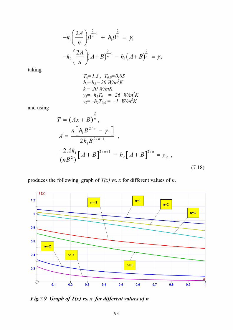
93

( ) ( )

2 21

1 1 1

2 212 2 2

2

2

n n

n n

Ak B h BnAk A B h A Bn

γ

γ

−

−

⎛ ⎞− + =⎜ ⎟⎝ ⎠⎛ ⎞− + − + =⎜ ⎟⎝ ⎠

taking T0=1.3 , T0,0=0.05 h1=h2 =20 W/m2K k = 20 W/mK γ1= h1T0 = 26 W/m2K γ2= -h2T0,0 = -1 W/m2K

and using

[ ] [ ]

2

2 /1 1

2 / 11

2 / 1 2 /12 22

( ) ,

,2

2 ,( )

n

n

n

n n

T Ax B

n h BA

k BAk A B h A B

nB

γ

γ

−

+

= +

⎡ ⎤−⎣ ⎦=

−+ − + =

(7.18) produces the following graph of T(x) vs. x for different values of n.

Fig.7.9 Graph of T(x) vs. x for different values of n

94

The total entropy production is calculated in the following way:

( ) ( ) ( )

( )

2 22( 1)2

2 12 221

21

1

2( ) '

2

n

t nn

n

A Ax Bk Ax Bk T nTT T Ax B

k AT n

σ

−

⎛ ⎞⎜ ⎟⎝ ⎠

⎛ ⎞ +⎜ ⎟+ ⎝ ⎠= =+

⎛ ⎞= ⎜ ⎟⎝ ⎠

Since n 2 2

1T ( (0) )A B B= + = then

214

tk An B

σ ⎛ ⎞= ⎜ ⎟⎝ ⎠

Equations (7.16) can be expressed as the function of ratio R=k/h in order to see how the values of k and h influence the solution. For k=20W/mK and R=k/h, values of total entropy production (W/K) for different values of n and R are shown in Table 7.9. Table 7.9

h n R

1 20

2 10

5 4

10 2

20 1

100 0.2

-5 11.8 31.7 87 16.1 2.5 1.9 -4 10.3 24.9 47 10.6 3.9 3.0 -3 8.8 19.7 34 19.8 9.0 5.9 -2 9.4 22.9 63 118 177 80.9 -1 13.9 34 101 218 459 2368 0 0.043 0.17 1.03 3.9 14.0 103 1 0.010 0.035 0.162 0.43 0.92 2.4 2 0.013 0.047 0.226 0.63 1.4 4.0 3 0.014 0.051 0.266 0.80 2.0 6.3 4 0.014 0.053 0.291 0.97 3.1 5.0 5 0.014 0.053 0.309 1.21 3.2 3.2

95

It is easy to see that for n=0, different solution is obtained and the different method of entropy production calculation is required. Using the solution

21

1

( )x

TT x TT

⎛ ⎞= ⎜ ⎟

⎝ ⎠

the following equations are obtained:

21 0 1

1

22 2 0 , 0

1

l n ( )

l n ( )

Tk T h T TTTk T h T TT

− = −

− = −

(7.19) Dividing the two equations by each other produces the following expression

2 0,02

1 0 1

T TTT T T

−=

−

and

1 0,02

1 02TT

TT T

=−

Substituting the above expression for T2 into first of equations (7.17) gives

0,01 0 1

1 0

-kT ln ( )2

Th T T

T T⎛ ⎞

= −⎜ ⎟−⎝ ⎠

which can be solved numerically for T1. Using k=20 W/mK, T0 = 1.3 and T0,0 = 0.05 gives T1=0.70773 and T2=0.30648 and

2 22

2

0.30648ln 20 ln 14.0 /0.70773t

Tk W KT

σ⎛ ⎞ ⎛ ⎞= = =⎜ ⎟ ⎜ ⎟

⎝ ⎠⎝ ⎠

96

8. Applications

As stated by Bejan [1]: Entropy Production Minimization is the method of thermodynamic optimization of real systems that owe their thermodynamic imperfections to heat transfer, fluid flow, and mass transfer irreversibilities. The method combines at the most fundamental level the basic principles of thermodynamics, heat and mass transfer and fluid mechanics and because of its interdisciplinary character, EGM is distinct from each of these classical disciplines.

The above statement indicates the possibility of some significant practical applications. This is indeed a case. The wide overview of the applications is presented by Bejan [1].

One of the first applications has been the determination of the units of

heat exchanger when the entropy production is minimized in the system as the result of two irreversible processes – flow with friction and heat transfer between two fluids across the finite temperature difference. Entropy production minimization allows to determine the optimal pipe diameter of the heat exchanger. These topics are well supported in literature (see Bejan [1], Chapter 4 and 5).

Another application involves problems with Insulation Systems both in

powers plants and in refrigeration plants (Chapter 6). The entropy production minimization method has also been used in the analysis of energy and exergy storage. An important application is also represented by the optimization of thermodynamic cycles in the contemporary power plants’ systems. The analysis is focused on the role of heat exchangers and the optimal combustion temperature. Bejan has shown that the maximum power of the electric power plant means the entropy production minimization.

An important range of applications is also reflected in the solar-thermal power generation, particularly in finding an optimal temperature of the solar collector which is working under non-isothermal conditions with the decreasing fluid temperature as the result of decreasing in time amount of sunshine.

Many important applications are also related to the problems of refrigeration which can be solved by designing an optimal system of heat exchangers and by selecting appropriate circulation parameters.

97

In addition to Bejan’s achievements, it is important to mention the application of the entropy production minimization method in describing the formation of the dissipative structures in life processes (see for example the work of Kirkaldy [12] concerning the thermodynamic explanation of human brain’ activity).

Large attention should also be paid to the work describing the metabolic processes or the diffusional coupling of the substance’s flow in sodium and potassium ions pumps across the organism’s single cell membranes [12]. The solutions, achieved in this thesis , of the entropy production problems in the processes of heat transfer with various boundary conditions , represent the theoretical basis of the entropy production minimization problems.

98

9. Summary

In the thesis, the applications of entropy production minimization method have been presented, in the stationary processes of heat conduction in solids and diffusional mass transfer.

It has been shown that these processes are described by the similar differential equations and boundary conditions and hence their methods of solving are, in principle, identical.

It has been established that the well known differential equations of Laplace and Poisson are the approximations resulting from assuming the average temperature across the entire region of the thermodynamic system. This has been demonstrated by the in depth analysis of the entropy production minimization according to Prigogine’s procedure. The general approach with calculus of variations allows to derive a full differential equation for the heat transfer. For example, when the heat conduction coefficient is constant, the calculus of variations approach leads to equation

22

2

1 0d T dTdx T dx

⎛ ⎞− =⎜ ⎟⎝ ⎠

(9.1) while the classical equation is

2

2 0d Tdx

=

in the one-dimensional system or

22 22 2 2

2 2 2

1 0T T T T T Tdx dy dz T x y z

⎡ ⎤⎛ ⎞∂ ∂ ∂ ∂ ∂ ∂⎛ ⎞ ⎛ ⎞+ + − + + =⎢ ⎥⎜ ⎟⎜ ⎟ ⎜ ⎟∂ ∂ ∂⎝ ⎠ ⎝ ⎠⎢ ⎥⎝ ⎠⎣ ⎦

and 2 2 2

22 2 2 ( , , ) 0T T T T x y z

dx dy dz∂ ∂ ∂

+ + = ∇ =

for the 3-D ortho-cartesian geometry.

99

The detailed interpretation of the second term in equation (9.1) has been presented as well as its agreement with the First and Second Laws of Thermodynamics. The boundary value problems have been formulated for all three kinds of boundary conditions including the most general conditions of Sturm-Liouville. The discussion has also focused on the method of solving general non-linear Euler-Lagrange equations. It has been demonstrated that the non-linear boundary problems, for any heat conduction coefficient with internal heat source, lead to the differential equation for heat transfer which can be further rearranged into the Bernoulli differential equation. This transformation permits to obtain, in spite of its non-linearity, an analytical solution which is often given in the non-explicit form. This is definitely a new contribution to the boundary problems with the entropy production minimization. The possible uses of the solution methods have been demonstrated by various numerical calculations. Another important achievement of this thesis is the demonstration of the method allowing for the calculation of the additional internal heat source and the entropy production rate in case of the non-explicit solutions. Finally, it has been explained that there is no direct link between Prigogine’s minimum entropy production in stationary processes and the entropy production minimization methodology. This derives from the important statement that the entropy production is path dependent and it can not be linked to the concept of entropy as the function of state.

100

Appendix 1 Principles of Calculus of Variations Calculus of Variations is concerned with finding the function y(x) such that the definite integral of the functional dependent on y(x) would reach the minimum. In case of one independent variable x and one dependent variable y(x), the problem reduces to finding the minimum of the integral:

2

1x

( , , ) minimumx

xF x y y dx ⇒∫ (A.1)

where yx = dy/dx. The integral limits are set and each dependent variable y(x1) and y(x2) have a set value. It can be shown [11] that the necessary condition for integral (A.1) to have a minimum, it must satisfy the following differential equation:

0x

F d Fy dx y

⎡ ⎤∂ ∂− =⎢ ⎥∂ ∂⎣ ⎦

(A.2) known as the Euler-Lagrange equation. In case of more independent variables, the problem focuses on finding the function u=u(x, y, z), such that the integral

2 2 2

1 1 1

,( , , , , , )x y z

x y zx y z

F x y z u u u u dxdydz∫ ∫ ∫

reaches the extreme value. In this case, the necessary condition for the minimum is met if the following Euler-Lagrange equation is satisfied:

0x y z

F F F Fu x u y u z u

∂ ∂ ∂ ∂ ∂ ∂ ∂− − − =

∂ ∂ ∂ ∂ ∂ ∂ ∂

(A.3)

101

If, in addition to function u(x,y,z), there are other dependent functions, then the necessary condition becomes a system of Euler-Lagrange equations. In practical applications, quite often, the problems arise in which the specific integral is expected to reach the extreme value while the additional conditions must be satisfied described as the integrals containing the same variables in the same domain of independent variables. This type problems are solved with the method of Langrange multipliers. One searches for the minimum of the integral

V

F d V∫

with the additional conditions

1 1 2 2 3 3, , ,.........., ,n nV V V V

FdV c F dV c F dV c F dV c= = = =∫ ∫ ∫ ∫

where dV represents the volume element of the multidimensional space and c1,c2,…..,cn are the known constants. The solution is determined by finding the minimum of the integral

V

K d V∫

where

1 1 2 2 ........ n nk F F F Fλ λ λ= + + + + . The necessary condition for the minimum is met if the following Euler-Lagrange equation is satisfied (for one independent variable):

0x

K d Ky dx y

⎡ ⎤∂ ∂− =⎢ ⎥∂ ∂⎣ ⎦

The unknown values of λi ( i = 1,2,3,…..,n) are found from the additional conditions. If the function F includes the derivatives of higher orders, the additional terms are included in the Euler-Lagrange equations.

102

References 1. Bejan, A. ; Entropy Generation Minimization, CRC Press, Boca Raton, 1995 2. Kondepudi, D. and Prigogine, I. ; Modern Thermodynamics , John Wiley and Sons, Chichester, 1998 3. Guminski, K. ; Termodynamika procesow nieodwracalnych , PWN, Warszawa, 1962 4. Bujakiewicz-Koronska, R.; Przemiany materii i informacji w strukturach dyssypatywnych , Rozprawa doktorska, Wydzial Fizyki i Techniki Jądrowej AGH, Krakow, 1997 5. Bejan, A. ; Heat Transfer , John Wiley and Sons, New York, 1993 6. Reif, F.; Statistical Physics , McGraw Hill Book Company, New York, Berkeley Physics Course – Vol.5, 1965 7. Szargut, J. ; Exergy Method, WIT Press, Southhampton, 2005 8. Rafois, I. and Ortin, J. ; Heat conduction in a metallic rod with newtonian losses, Am. J. Phys. 60 (9), September 1992 9. Kleidon, A. and Loretz, R.D. (Eds.) ; Non-Equilibrium Thermodynamics and the Production of Entropy, Springer, Berlin, 2005 10. Kolenda, Z. et all ; On the minimum entropy production in steady state heat conduction processes, Energy , Elsevier, 29, 2004 11. Martin Becker ; The Principles and Applications of Variational Methods, Research Monograph No 27, The M.I.T. Press, Cambridge, 1964 12. Kirkaldy, J.S. ; The Thermodynamics description of heterogeneous dissipative systems by variational methods, Part III, Can.J.Phys. 42, 1964, 1437-46 and Part II, 38, 1960, 1356-66