table of contents page - auburn university › academic › classes › biol › 3060 › dobson ›...
TRANSCRIPT

ZOOLOGY 306
PRINCIPLES OF ECOLOGY
WINTER 1999
COURSE PACK
Table of Contents Page
Course description 3
Syllabus 6
Outline of Principles of Ecology 8
Introduction 8
Ecology as a Science 9
World Climate 9
Soils as Environments 10
Landscape Ecology 10
Physiological Ecology 11
Evolutionary Ecology 12
Behavioral Ecology 12
Population Ecology 13
Life History 14
Interactions Between 2 Species 15
Competition 15
Predation 15
Community Dynamics 16

Ecosystem Ecology 17
Ecology Papers
Content Guidelines 19
Example Paper 21
LABORATORYEXERCISES
#1: Population SizeEstimation Using AquaticSnails
25
#2: Distribution of a PlantParasite on its Host
31
#3: Constructing LifeTables for Homo sapiens
40
#4: Community Diversityof Stream Fish
44
Data Sheets 51
Winter 1998 Examinations
Hour Exam I 55
Hour Exam II 60
Final 65
ZOOLOGY 306 -- PRINCIPLES OF ECOLOGY -- WINTER 1999
Instructors - F. Stephen Dobson (320 FS, office hours to be announced); Paul Nolan, AnneFord, Andrew Stoehr (offices and office hours to be announced).
Course pack - available at Sofy copy for less than $10.00. The course pack is required.
Texts - There is no required text! If you have a serious interest in the science of ecology, now orlater on, I suggest that you buy a copy of "Ecology: Individuals, Populations, and Communities,3rd Edition" by Begon, Harper, and Townsend (1996, Blackwell Scientific Publications), and useit as a reference book. If you are interested in ecology within the context of environmentalscience, you might want to look at "Ecology of a Changing Planet" by Bush (1997, PrenticeHall).
Lecture - Lectures are from 8-9 am MTWH, in 336 Funchess Hall.
Laboratory - Laboratory sections begin during the 2nd week of classes. The laboratory part ofthe course meets once a week (rain or shine) for 3 hours in the afternoon (2-5 pm on M, T, W,and H) in 336 Funchess Hall. There will be four laboratory projects during the quarter, eachtaking two or three of the weekly lab periods. Descriptions of the laboratories are included in thiscourse pack. Please read the lab write-up for the week before you come to lab. Twolaboratory reports are required, and these will be written in the format of a scientific paper. Thelaboratory reports must be produced on a word processor. The 1st report will be on the initiallab exercise, and is due in class at the beginning of lecture on Thursday, 4 February. Five pointsare deducted from the total possible points for reports for each class day late, and incompletepapers are not acceptable. After the 1st report is graded and returned, you can submit a rewrite aweek later to receive a re-grade. Points off for late papers come off the top of your score, andcannot be made up! The 2nd report can be on either the second or the third lab. There will be norewrite of the 2nd report. The 2nd lab report is due at the beginning of lecture on Thursday, 4March. "Dual" reports that are similar in prose will be handed back with a grade of zero.Copying verbatim from the course pack or any other literature source is not acceptable.Also, we will not accept lab reports for a laboratory for which you have an unexcusedabsence. There will be at least one question from the fourth lab on the final examination.
Each laboratory has two parts. In the first week or two of a lab, you will collect original data inthe field. In the final (usually second) period of a lab a week later, you will analyze the data thatyou collected, and from the results make conclusions about ecological questions. Basically, youwill be doing ecological research projects. The lab instructor will be present during all labs tohelp and guide you in this process, and all of the instructors are happy to help you decide how towrite the lab reports.
The field part of the labs will be done outdoors and is intended to encourage you to think aboutplants and animals in their environment, and to think about how to investigate ecologicalquestions. Be aware of the hazards of the outdoors. Protect yourself against sunburn and bitesand stings of insects. If you are allergic to bee stings, tell your lab instructor (bring theappropriate medication to your lab section, and tell us where you keep it, in case you are stung).
Equipment - Data sheets are provided on pages 51 to 54 of this course pack. Bring pencils andpaper for note-taking to the labs, and also a clip-board with protective cover, and rain gear

(raincoat or poncho and water-proof footgear) for working outside in the rain. If you havehipboots, you will probably want to bring them to both field weeks of the first lab, and to thefield week of the last lab. If you don’t have hipboots, bring a towel to dry off with after workingin streams, and some dry shoes and socks.
Grades - Grade points are divided up as follows:
2 hour exams @ 100 pts each 200 points 40%
Final exam 200 40%
2 lab reports @ 50 pts each 100 20%
Total Points 500 100%
Grading policy - The following are the maximum standards for assigning grades. Final gradingmay be slightly easier (a lower point level accepted; e.g., an 79.9% might be accepted as a B) forany category, at my discretion.
A 90-100.0% 450-500 points
B 80-89.9% 400-449 points
C 70-79.9% 350-399 points
D 60-69.9% 300-349 points
F Below 60% Below 300 points
Exams - Questions on exams can cover any of the lectures, any class handouts, or any laboratorymaterial that was presented before the day of the exam. Thus, the 2nd exam and final arecumulative, though they will emphasize more recently covered material. The 1st exam will beduring the lecture period on Thursday, 28 January, and the 2nd exam during the lecture period onThursday, 18 February. The final will be from 11:00am -1:30pm on 16 March (Tuesday) in 336Funchess Hall. If you have to miss an exam, you must submit a signed note (e.g., from aDoctor, Dean, or Coach). If you have an unexcused absence from an exam, you get a 0!
NOTICE ABOUT EXAMS: To help you prepare for the exams, there is a copy of the examsfrom the Winter quarter of 1998 at the end of this course pack on pages 55 to 74. Looking overthe old exams is especially helpful because there is time pressure on all of the exams.
Attendance policy - Lecture attendance is not recorded (there are just too many of us!), but youare urged to attend regularly. You are responsible for any and all announcements made in

lecture, so if you miss a lecture you might want to check with someone for the news. You willbe tested primarily on the lecture material, and you should plan to borrow notes from a colleagueif you have to miss a lecture. My attendance policy is based on the fact that you are an adult, andhave the right to decide for yourself whether to attend the lectures. Ecology is lots of fun,however, and you are most likely to enjoy the course, get a good grade, and learn lots ofinteresting ideas and concepts if you don't miss a single minute!
The laboratory is the most fun part of the course, and an important part of the "experience." Youwill be analyzing data that the whole class collects, so we all depend on each other in lab.Because of this, lab attendance is required. In order to do well on the lab quizzes (20% of yourgrade), you will want to attend labs anyway. Remember that questions on material coveredduring the labs are fair game for the lecture exams, and there will be a quiz on the last lab projectattached to the final exam.
NOTICE: you will lose 10 points for each lab for which you have an unexcused absence.The points will be subtracted from your point total before final grades for the course areassigned.
SYLLABUS
DATE TOPIC
5-Jan Introduction
6 Ecology as a Science
7 Ecology as a Science
LAB: no lab the 1st week of class
11 World Climate
12 World Climate
13 World Climate
14 Soils as Environments
11-14 LAB: population estimation (in the field)

18 MARTIN LUTHER KING DAY
19 Landscape Ecology
20 Physiological Ecology
21 Physiological Ecology
18-21 LAB: population estimation (in the field)
25 Physiological Ecology
26 Physiological Ecology
27 Evolutionary Ecology
28 HOUR EXAM I
25-28 LAB: population estimation (in Funchess)
1-Feb Evolutionary Ecology
2 Evolutionary Ecology
3 Evolutionary Ecology
4 Behavioral Ecology
(1st lab report due, at 8:10am in lecture)
1-4 LAB: midge gall distribution (in the field)
8 Behavioral Ecology
9 Population Ecology
10 Population Ecology
11 Population Ecology
8-11 LAB: midge gall distribution (in Funchess)

15 Population Ecology
16 Life History
17 Life History
18 HOUR EXAM II
15-18 LAB: human life table (in the field)
22-Feb Life History
23 Life History
24 Competition
25 Competition
22-25 LAB: human life table (in Funchess)
1-Mar Competition
2 Predation
3 Predation
4 Community Dynamics
(2nd lab report due, at 8:10am in lecture)
1-4 LAB: stream fish diversity (in the field)
8 Community Dynamics
9 Community Dynamics
10 Ecosystem Ecology
11 Overview

8-11 LAB: stream fish diversity (in Funchess)
16-Mar FINAL EXAM, at 11:00am - 1:30pm, in 336Funchess Hall
OUTLINE OF PRINCIPLES OF ECOLOGY
INTRODUCTION
Overview of the course.
A. Ecology is a science.
B. World climate.
1. Elements of climates.
2. Climates and geography.
C. Soils as environments.
1. Interaction of soil and water.
2. Biotic and abiotic factors in soils.
D. Landscape Ecology.
1. Biomes.
2. Ecoclines.
E. Physiological ecology.
1. Studies of "how" questions.
2. The niche.
3. Animal responses to temperature.
4. Influences on distributions.

F. Evolutionary ecology.
1. Studies of "why" questions.
2. Measuring natural selection.
3. Sexual selection.
G. Behavioral ecology.
1. Evolution of behavior.
2. Sexual selection (revisited).
3. Mating systems
H. Population ecology.
1. Population growth.
2. Regulation of population size.
3. Demography.
4. Life-history theory.
I. Interactions between two species.
A. Competition.
B. Predation & parasitism.
C. Mutualism.
J. Community dynamics.
1. Species diversity.
2. Trophic levels.
3. Complex interactions.
4. Succession = community development.
K. Ecosystem ecology.
1. Energy flow.
2. Biogeochemical cycles.
Ecology as a Science
I. What is ecology?
A. Ecology = "oikos" = house.
B. Definitions.
1. Haeckel (1869): the total relations of the animal to both its organic and itsinorganic environment.
2. Elton (1927): "scientific natural history".
3. Odum (1959): "science of the living environment".
4. Krebs (1985): "the scientific study of the distribution and abundance oforganisms".
5. Ecology = the scientific study of the interactions of organisms with theirenvironments".
C. Ecological systems are dynamic.
D. Abiotic & biotic components of the environment.
E. Pattern & process
II. The scientific method.
A. The search for pattern - natural history.
B. Induction & deduction.
C. The hypothetico-deductive method.
1. Gather data.
2. Search for pattern.
3. Form hypothesis.
4. Derive predictions.
5. Empirical tests: gather new data.
6. Evaluate:
a. accept/reject predictions and ...
b. support/falsify hypothesis.

D. Reductionism & holism.
I. Why is climate important in ecology?
A. Elements of climate.
1. Sun.
2. Wind.
3. Water.
B. Solar radiation.
C. Temperature patterns.
D. Greenhouse Effect
E. Air currents.
F. Coriolis Force.
G. Ocean Currents.
H. Precipitation patterns.
1. Adiabatic Cooling & Heating = change in temperature but not in "total heatcontent".
2. Warmer air holds more moisture.
II. Climate and geography.
A. Land masses.
B. Elevation and latitude.
C. Influences of mountains
1. North and south facing slopes.
2. The "rain shadow" effect.
D. Maritime vs continental climates.

E. Temperate vs tropical seasons.
III. Example of climatic influences on organisms.
A. El Niño and Darwin's finches.
Soils as Environments
I. Interaction of soil and water.
A. Precipitation and soil water.
B. Water retention in soil.
1. Field capacity = water held against gravity.
2. Wilting point = unavailable water bound by soil.
3. Available water = field capacity - wilting point.
II. Interaction of physical and biotic factors in soils.
A. Components of soil.
B. Soil formation: primary succession.
C. Examples of soil types.
1. Podzol in northern spruce forests.
2. Brown earth in temperate deciduous forests.
3. Chernozem in temperate grasslands.
Landscape Ecology

I. What is landscape ecology?
A. Definition: study of patterns of land form and biota (e.g., biomes) over a broad rangeof spatial scales.
B. Five areas of study in landscape ecology.
II. What is a biome?
A. Definition: broad structural classes of communities or ecosystems based primarily onthe growth forms of the plants present and characteristics of climate.
B. Dominant growth form = life-form of plants (viz., herbs, shrubs, trees).
C. Major determinants of biome-types: precipitation & temperature.
D. Trends in plant characteristics.
III. What is an ecocline?
A. Definition: dramatic vegetation change along an environmental gradient on aglobal scale.
B. Ecoclines.
a. Deciduous forest to desert.
b. Up a mountian at the equator.
c. Tropical rainforest to desert.
Physiological Ecology
I. Liebig's "Law of the Minimum" = limiting factors on ecological processes (e.g.,growth or reproduction).
II. Shelford's "environmental tolerance" = limiting factors can be under-abundantor over- abundant.

A. Tolerance curves.
B. Acclimation and acclimatization = "gearing" to different environmentalconditions.
III. Grinnell & Hutchinson: niche = total range of conditions under which anindividual lives and replaces itself.
A. Hypervolume model (more than 3 environmental axes).
a. Types of niches.
i. Fundamental niche = where individual can live and reproduce.
ii. Realized niche = where individual does live and reproduce.
IV. Animal responses to temperature.
A. Heat budgets.
B. Body temperatures.
1. Poikilotherm = body temperature similar to that of the external environment.
Homeotherm = body temperature maintained constant through oxidativemetabolism.
2. Conformers & regulators.
3. Ectotherm = body heat obtained from external environment.
Endotherm = body heat produced internally.
4. Body size effects.
C. Metabolic costs of homeothermy.
1. Thermal neutral zone.
2. Basal metabolic rate.
3. Upper and lower critical temperatures.
V. Physiological influences on distributions.
A. Timberline.

1. Freeze drought.
2. Ecotone = sharp boundary between 2 major communities.
B. Northern limits of wintering U.S. birds.
Evolutionary Ecology
I. Questions that ask how? & why?
A. Are evolutionary questions important?
B. What is evolution?
1. Change in gene frequency.
2. Mechanisms: mutation, gene flow, drift, selection.
II. Evolution by natural selection.
C. Conditions for Natural Selection
1. Variation.
2. Fitness differences.
3. Inheritance.
4. Outcome - change in trait frequency.
B. Example: Industrial Melanism of Pepper Moths.
C. Discontinuous and continuous traits.
D. Forms of natural selection.
1. Directional.
2. Stabilizing.
3. Disruptive.
III. Evolutionary ecology in action.
A. Oscillating selection.

B. Adaptation: becoming suited to survive & reproduce.
IV. What is sexual selection?
A. Sexual dimorphisms.
B. Limiting sex & limited sex.
C. Components of sexual selection.
1. Intrasexual competition for mates.
2. Epigamic selection = mate choice.
3. Fisher's "runaway" sexual selection.
D. Where does sexual selection stop?
1. Fisher's "balance."
2. "Good genes" models.
Behavioral Ecology
I. What is behavioral ecology?
A. Behavioral traits & environmental circumstances.
B. Ecological & social environments.
C. The evolution of behavior.
1. Kin selection & altruism.
2. Cost/benefit analysis.
II. Mating systems & sexual selection.
A. Predicting sexual dimorphism.
B. Tests with mammalian sexual size dimorphism.

III. Types of mating systems.
A. Mating system = the general behavioral strategy employed in obtaining mates.
B. Basic types of mating systems.
1. Monogamy.
2. Polygyny.
3. Polyandry.
4. Promiscuity.
C. Behavioral characteristics of mating systems.
D. Constraints on mating patterns.
IV. Monogamy or polygyny: Orians' "polygyny threshold" model.
Population Ecology
I. Population: a group of organisms coexisting at the same time and place and capablefor the most part of interbreeding.
A. The estimation of population size.
B. Unitary & modular organisms.
C. Distributions of individuals.
1. Regular or even.
2. Random.
3. Contagious, patchy, clumped or aggregated.
D. Methods of estimation.
1. Counts & projections.
2. Estimates of abundance.
3. Relative indices of abundance.

II. How do populations change over time?
A. N0+1 = N0 + B + I - D - E
B. Assumptions of our 1st population model.
1. Unlimited environment.
2. Environment is evenly distributed.
3. Reproduction at discrete intervals & non- overlapping generations.
4. Partial individuals possible.
5. Individuals are ageless, and equal in their effects on population size.
6. Population only defined at discrete intervals.
7. No dispersal.
C. Exponential population growth.
1. Model 1: discrete exponential growth.
a. R0 = (1+b-d) = the net reproductive rate of the population.
b. Population growth is geometric.
2. Model 2: continuous exponential growth.
a. lnR0 = r.
b. r = the instantaneous rate of natural increase.
c. dN/dt = rN
3. Examples of exponential growth.
a. Reindeer on Saint Paul Island in Alaska.
b. Nesting gannets in Great Britain.
D. Logistic population growth: Model 3.
1. Relaxing the assumption of an unlimited environment.
2. K = the carrying capacity of the environment.
3. Assuming a linear decrease in r.
4. dN/dt = r(1-N/K)N = r[(K-N)/K]N.
5. Examples from the laboratory & nature.
III. The study of population "regulation."
A. Factors that limit population size.
1. Predation.
2. Food Resources.
3. Weather patterns.
B. Example: Columbian ground squirrels.
C. Density-dependence and density independence.
Life History
I. What is demography?
A. Rates of birth, death, immigration, and emigration.
B. Age structure.
II. Predicting populations from demography.
A. Assume immigration = emigration.
B. Focus on births and survival.
C. Survival curves.
D. Population pyramids.
E. Life tables.
1. Survival & mortality.
2. Fecundity = mean # offspring/individual.
3. Stable age distribution.
4. Net reproductive rate = R0 = Σ lxmx.

5. Generation length = G = T = Σ xlxmx/R0.
6. Intrinsic rate of natural increase = r = lnR0/G.
III. Life-history theory.
A. Patterns of reproduction, growth & survival.
B. Intraspecific & interspecific.
C. Energy tradeoffs.
1. Reproductive effort.
2. Somatic effort.
C. The r-K selection model.
1. Fluctuating environments.
2. Stable environments.
D. The bet-hedging model.
1. The "bad years" effect.
2. Predictions differ from r-K selection.
Interactions Between Two Species
I. Competition [- -].
A. The nature of competition.
1. Gause's laboratory experiments.
a. The competitive exclusion principle.
b. The principle of limiting similarity.
2. Mechanisms of competitive interaction.
a. Exploitation competition.
b. Interference competition.
c. Guild = similar species that share a common resource.

d. Hutchinson's 1.3X body size relationship.
B. Lotka-Volterra model.
1. Logistic population growth.
2. Coefficients of competition.
3. Graphic representation.
a. Looking for the equilibrium point.
b. Isoclines for competitors.
c. Four outcomes.
C) e.g., Darwin's finches.
1. Character displacement = increased differences between species where they occurtogether.
2. Patterns that support character displacement.
a. Pattern found by David Lack.
b. Study of food resources.
II. Predation & parasitism [+ -].
A. The nature of predation.
1. Common predation.
2. Herbivory.
3. Parasitism.
4. Batesian mimicry.
B. Examples of predation.
1. Gause's laboratory experiments.
2. Lynx-hare cycle.

a. Refuges.
b. Switching.
C. Lotka-Volterra model of predation.
1. Births and deaths of the prey.
2. Births and deaths of the predator.
3. Predator-prey cycle (revisited).
D) Additional principles.
1. Functional & numerical responses of predator.
a. Functional response = each predator eats more.
b. Numerical response = predator population increases.
2. Limitation of prey populations.
III. Mutualism [+ +]
IV. Commensalism [+ 0]
V. Amensalism [- 0]
VI. Neutralism [0 0]
Community Dynamics
I. Community level properties: the holistic viewpoint.
A. Are communities natural units?
B. Clements: succession to monoclimax.
1. Succession = community development.

2. Climax community = the ultimate community that will occur under given climaticconditions.
3. Monoclimax (= climatic climax) = only one climax community possible under givenconditions.
4. The community as a cybernetic (= self governing) superorganism.
C. Gleason: the individualistic hypothesis.
1. Each community is unique.
2. Any of several climax communities are possible.
D. The test: Whittaker's results.
II. Measures of species diversity.
A. S = species richness = # of species.
B. Importance curves.
C. H' = Shannon-Wiener Index = -Σ pi • lnpi .
D. J = evenness = H'/lnS.
E. Diversity gradients.
III. Structuring communities: equilibrium mechanisms.
A. Competition.
1. Reducing resource overlap: trophic apparatus.
2. Trophic = pertaining to food or nutrition.
3. Temporal reduction of resource overlap.
4. Specialists & generalists.
5. Niche packing = community of several specialists.
6. Guild = similar species with similar resources (reminder).
7. Example of Bombus species.
B. Predation.
1. Trophic level = position in a food chain.

2. Food chain (or food web) = the way that energy passes through populations in acommunity.
3. Producers, 1° consumers & 2° consumers.
4. Ontogenetic niche = feeding niche changes during growth and development.
5. Keystone predation = predation that promotes coexistence among competitors.
6. Example of starfish in the intertidal zone.
IV. Structuring communities: non-equilibrium mechanisms.
A. Historical Factors
B. Periodic disturbance.
1. Disasters = regular, predictable disturbances.
2. Catastrophes = unpredictable disturbances.
3. The intermediate disturbance hypothesis.
V. Measures of community stability.
A. Numerical stability = no change in individuals when environment changes.
B. Elastic (adjustment) stability = community changes when environment changes, butthen returns to original state.
C. Persistence = # of individuals changes permanently, but # of species stays the samewhen environment changes.
D. Instability = extinction (local, total, ecological)
E. Global stability & local stability.
Ecosystem Ecology
I. Ecosystem = the sum total of abiotic and biotic factors in a given place.
A. Energy & nutrient transfers between trophic levels.

B. Primary producers (plants) = autotrophs.
C. Consumers (herbivores, carnivores, detritivores) = heterotrophs.
D. Net production = gross production - respiration.
II. Trophic efficiencies.
A. Consumption efficiency (CE) = energy absorbed/energy available
B. Assimilation efficiency (AE) = energy assimilated/energy absorbed
C. Production efficiency (PE) = net production/energy assimilated
D. Ecological efficiency = CE • AE • PE.
E. Ecological pyramids.
III. Biogeochemical cycles.
A. Components: structural elements, macronutrients, micronutrients.
B. Example: the nitrogen cycle.
ECOLOGY PAPERS -- CONTENT GUIDELINES
Title
Is it indicative of the study?
Abstract
a. Purpose of study
b. Site, study species
c. Estimation methods
d. Results Summary (#'s)
e. Discussion Statement

Introduction
a. Background Information
-why is population estimation important?
-what are some ways in which population estimates might be used?
b. Purpose of study
-what methods were compared?
-why examine different methods?
-what is the take home message of the experiment?
c. Hypothesis and/or predictions
-stated clearly and concisely.
Methods
a. Site description
-where, when, how?
Chewacla Creek, area (cm2, m2, km2, whatever's appropriate) temps,maximum depths, bottom, dates (including year), weather, materials (if it'snot obvious)
b. Study animal
-why was it appropriate?
Life history, reproduction rate, movement patterns, ease/safety of capture
c. Search effort
-specific description of how the experiment was carried out
d. Estimation methods
-how was estimate derived?
Include relevent formulas, w/description of terms.
-assumptions? (could also be covered in discussion)
Results

a. Enumeration--total
b. Mark/Recapture--based on recapture rates of each color, and overall
c. Depletion--one for each week, plus graph(s) with fully descriptive caption(s)
Discussion
a. Fulfill the purpose you described in the Introduction
b. Which method was most reliable, and why?
c. For each method:
-which assumptions were violated?
-how does this affect the estimate?
-what could be done to improve the outcome next time?
d. What was the overall conclusion about estimation methods & theiruse/usefulness?
Format
a. Did the paper follow the scientific format? Use metric units? Have A LiteratureCited section?
b. Double spaced, typed, stapled
c. grammar, spelling
d. Was there overlap between sections? Was everything where it was supposed tobe?
e. Style. Was it easy to understand? Was it logical and well argued? Clear &concise?
ESTIMATION OF POPULATION SIZE USING AQUATIC SNAILS
To understand how different physical or biological factors influence the distribution orabundance of species, we often need to measure changes in population size over space or time.However, it usually is not possible to obtain a complete count or census of a natural populationof animals (and it is often difficult even for plants!). For this reason, ecologists generally have torely on some kind of estimate of abundance or density. For example, one may have to count thenumber of singing males of a species of bird in a given community and then estimate the size of

the breeding population by assuming that for every male there is one female. Or one may countthe individuals in a sample area and then extrapolate to the larger area in which the wholepopulation lives. Because each method of estimating population size has different assumptions,and hence, different strengths and weaknesses, it is recommended that at least two methods beused and compared in any population study.
In this field lab you will estimate the abundance of aquatic snails that live in a stream inChewacla State Park. You will use and compare 3 different techniques for estimating populationsize: enumeration, depletion, and mark and recapture. In particular, you will be examining theassumptions of each method and their validity for this population. Population size may dependon local environmental factors, so be sure to keep your eyes open at the stream for factors thatmight affect the snails, and make some notes.
Snail Biology
You will be estimating population size of the yellow Elimia (Elimia taitiana), an oviparous (egglaying) snail of the family Pleuroceridae. Elimia are common inhabitants of rocky shoals ofstreams and rivers throughout much of the eastern half of the United States. These snails belongto the sub-class Prosobranchia, which breathe by means of an internal gill and which have anoperculum that can close off the entrance to the shell. The sexes are separate, unlike the subclassPulmonata (which breathes by means of a pulmonary sac, and has no operculum) where theindividuals are hermaphroditic (i.e., have both male and female organs in each individual). Snailsfeed by scraping algae and detritus off of the surface of rocks with a rough abrading devicecalled a radula. In the Pleuroceridae the radula has a central tooth.
The population biology of snails makes them great subjects for studying population size. Fromday to day, their range covers only a few square meters of area. They are easy to catch, and easyto mark (see below) and observe. They can live for a few years, and population sizes do notchange dramatically from day to day. Perhaps most important, yellow elimia are abundant, soestimates of their population size can be based on fairly large samples of individuals. They are anative species, and occur in fairly natural environments (that is, habitats that are undisturbed byhuman activities).
I. Enumeration
The simplest way to estimate population size is to count the number of individuals that youcapture. This can be done over several sampling periods, as we are going to do. It is oftenobvious, however, that some individuals are present in a study area and are not captured. Thus,the enumeration method provides a minimum estimate of population size, and is sometimescalled "the minimum number known alive." The enumeration method, if used for populationestimation, actually assumes that all individuals were captured, and that the removal of thecaptured individuals did not attract more individuals into the vacated study area (i.e., nomigration). If migration into the habitat occurs due to lower density as the captured individuals

are removed (even temporarily), this is termed a "vacuum" effect. The method also assumes thatno individuals are born or die during the period over which sampling is done.
II. Mark and Recapture
The mark and recapture method involves marking a number of individuals in a naturalpopulation, returning them to that population, and subsequently recapturing some of them. Thisprovides a basis for estimating the size of the population at the time of the marking and release.This procedure was used by C.J.G. Petersen in studies of marine fishes and F.C. Lincoln instudies of waterfowl populations, and is often referred to as the Lincoln Index or the PetersenIndex. It is based on the principle that if a proportion of the population was marked in some way,returned to the original population and then, after complete mixing, a 2nd sample was taken, thenumber of marked individuals in the 2nd sample would have the same ratio to the total number inthe 2nd sample as the total of marked individuals originally released would have to the totalpopulation. That is:
R/C = M/P
Where R is the number of marked animals recaptured in the 2nd sample
C is the total number of animals captured in the 2nd sample
M is the number of animals marked and released in the 1st sample
P is the (as yet unknown) population size
The accuracy of this method depends on a number of assumptions, including the following:
1) During the interval between the preliminary marking period and the subsequentrecapture period, nothing has happened to upset the ratio of marked to unmarked animals(that is, no new individuals were born or immigrated into the population and none died oremigrated).
2) All individuals are equally likely to be caught within each capture period. That is,marked individuals must not become either easier or more difficult to catch during thesecond capture period compared to unmarked individuals.
3) Sufficient time must be allowed between the initial marking period and the recaptureperiod for all marked individuals to be randomly dispersed throughout the population (sothat assumption 2 above is not violated). However, the time period must not be so longthat assumption 1 breaks down.
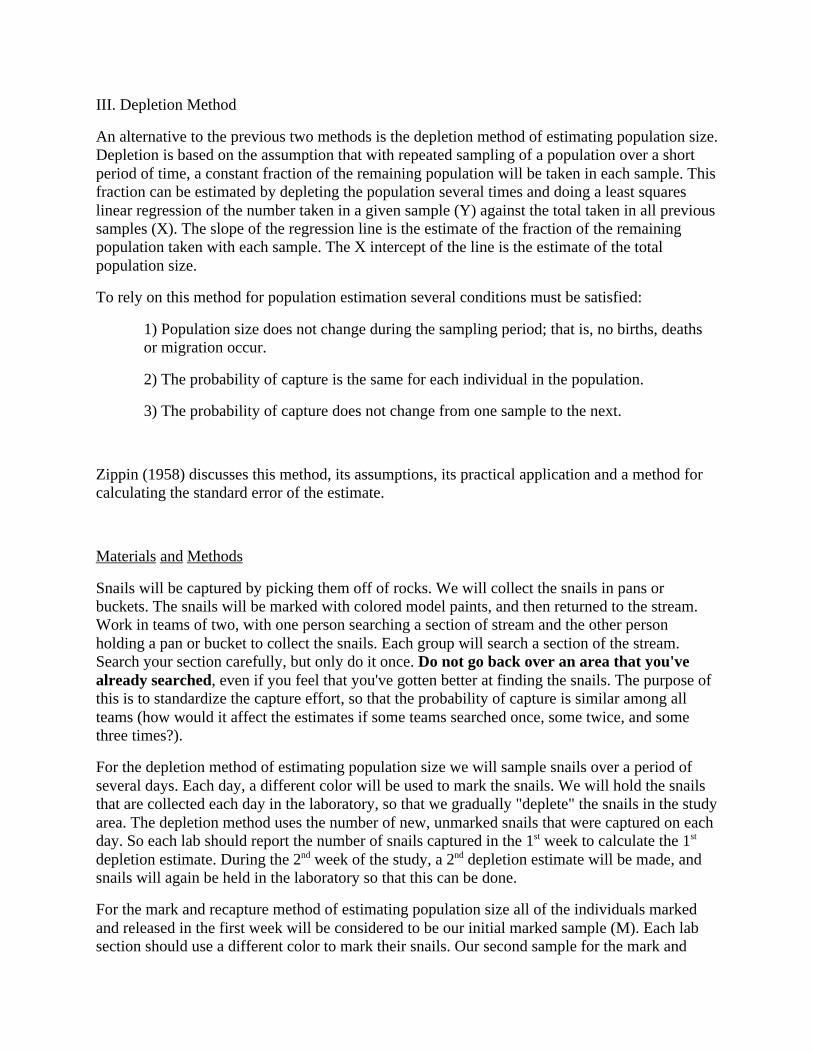
III. Depletion Method
An alternative to the previous two methods is the depletion method of estimating population size.Depletion is based on the assumption that with repeated sampling of a population over a shortperiod of time, a constant fraction of the remaining population will be taken in each sample. Thisfraction can be estimated by depleting the population several times and doing a least squareslinear regression of the number taken in a given sample (Y) against the total taken in all previoussamples (X). The slope of the regression line is the estimate of the fraction of the remainingpopulation taken with each sample. The X intercept of the line is the estimate of the totalpopulation size.
To rely on this method for population estimation several conditions must be satisfied:
1) Population size does not change during the sampling period; that is, no births, deathsor migration occur.
2) The probability of capture is the same for each individual in the population.
3) The probability of capture does not change from one sample to the next.
Zippin (1958) discusses this method, its assumptions, its practical application and a method forcalculating the standard error of the estimate.
Materials and Methods
Snails will be captured by picking them off of rocks. We will collect the snails in pans orbuckets. The snails will be marked with colored model paints, and then returned to the stream.Work in teams of two, with one person searching a section of stream and the other personholding a pan or bucket to collect the snails. Each group will search a section of the stream.Search your section carefully, but only do it once. Do not go back over an area that you'vealready searched, even if you feel that you've gotten better at finding the snails. The purpose ofthis is to standardize the capture effort, so that the probability of capture is similar among allteams (how would it affect the estimates if some teams searched once, some twice, and somethree times?).
For the depletion method of estimating population size we will sample snails over a period ofseveral days. Each day, a different color will be used to mark the snails. We will hold the snailsthat are collected each day in the laboratory, so that we gradually "deplete" the snails in the studyarea. The depletion method uses the number of new, unmarked snails that were captured on eachday. So each lab should report the number of snails captured in the 1st week to calculate the 1st
depletion estimate. During the 2nd week of the study, a 2nd depletion estimate will be made, andsnails will again be held in the laboratory so that this can be done.
For the mark and recapture method of estimating population size all of the individuals markedand released in the first week will be considered to be our initial marked sample (M). Each labsection should use a different color to mark their snails. Our second sample for the mark and

recapture technique will be obtained during the second week of the study. You may also want touse captures from each lab section to get several mark and recapture estimates of population size.Estimates can also be made for each of the different colors that were used to mark the snails (thisis why we use a different color to mark the snails each day).
To mark the snails, wipe the ventral (under) surface of the shell as dry as possible and place in apan for air drying. Mark the snails with a large clearly visible dot of paint. Allow the marks todry thoroughly before putting the snails in the laboratory bucket. Don’t let the snails go! We willtake them back to campus and hold them for a few days. At the end of the week, snails from allof the lab sections will be returned to the creek. After marking the snails, estimate the size of thearea sampled. A meter tape will be provided. Record the total number of snails collected by thelab section and the area of the stream that they were taken from. Also, record habitatcharacteristics (e.g., shade, current, bottom composition, etc.).
Equipment
Pans and buckets
Paints for marking
Meter tape
Clothing and shoes suitable for getting wet and muddy, towel, and dry socks andshoes (note: these last items really are essential, because good ecologists makesure that they'll be in good health for more work tomorrow!)
Hipboots if you have them
Data Analysis
Calculate the mark and recapture estimate using numbers of snails captured from week to week.Then do the same calculations for each color. The formula for the estimate is: P = (CM)/R (seeabove). Divide your estimates of population size by the area of stream that you sampled to get anestimate of population density.
Calculate a regression line using the total taken in all previous samples as the independentvariable (X), and the number taken in the current sample as the dependent variable (Y); see thecalculator handout for how to do a regression. The X-intercept of the regression line gives thepopulation estimate. The X-intercept is equal to -a/b, where a is the Y-intercept and b is the slopeor regression coefficient.
The following table shows some hypothetical results of four consecutive depletions of the samearea, and illustrates how to calculate the population estimate:
Sample # Total taken in # taken in this (X)*(Y)
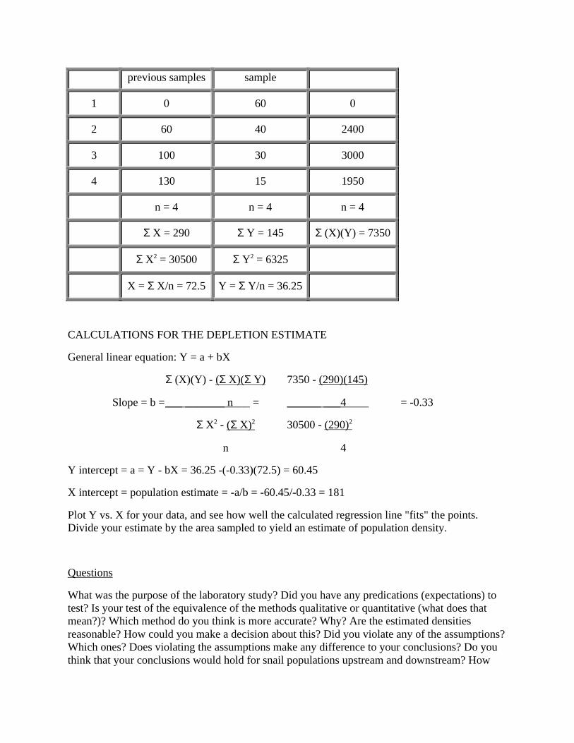
previous samples sample
1 0 60 0
2 60 40 2400
3 100 30 3000
4 130 15 1950
n = 4 n = 4 n = 4
Σ X = 290 Σ Y = 145 Σ (X)(Y) = 7350
Σ X2 = 30500 Σ Y2 = 6325
X = Σ X/n = 72.5 Y = Σ Y/n = 36.25
CALCULATIONS FOR THE DEPLETION ESTIMATE
General linear equation: Y = a + bX
Σ (X)(Y) - (Σ X)(Σ Y) 7350 - (290)(145)
Slope = b =___ _______ n___ = ______ ___4____ = -0.33
Σ X2 - (Σ X)2 30500 - (290)2
n 4
Y intercept = a = Y - bX = 36.25 -(-0.33)(72.5) = 60.45
X intercept = population estimate = -a/b = -60.45/-0.33 = 181
Plot Y vs. X for your data, and see how well the calculated regression line "fits" the points.Divide your estimate by the area sampled to yield an estimate of population density.
Questions
What was the purpose of the laboratory study? Did you have any predications (expectations) totest? Is your test of the equivalence of the methods qualitative or quantitative (what does thatmean?)? Which method do you think is more accurate? Why? Are the estimated densitiesreasonable? How could you make a decision about this? Did you violate any of the assumptions?Which ones? Does violating the assumptions make any difference to your conclusions? Do youthink that your conclusions would hold for snail populations upstream and downstream? How
could you make a stronger test of whether the methods are equivalent?
References
Southwood, T. R. E. 1978. Ecological methods, with particular reference to the study ofinsect populations, 2nd edition. John Wiley & Sons, Inc. New York. 524 pp.
Zippin, C. 1958. The removal method of population estimation. J. Wildlife Management22(1): 82-90.
Krebs, C. J. 1989. Ecological Methodology. Harper & Row, New York. pp. 15-63.
DISTRIBUTION OF A PLANT PARASITE ON ITS HOST
In this lab at the Tuskegee National Forest, we will examine the distribution of a plant parasiteon its host species. The lab has two purposes. First, the lab introduces you to methods foranalyzing the spatial distribution of organisms. Second, the lab should help you to gain insightsinto what factors may be influencing the distribution of an organism within its habitat.
Plant Galls and Gall Makers
We will not be looking at plant parasites directly in this lab, but rather at structures they form,called galls, on their host plants. Galls are growths on plants that are induced by parasiticorganisms. The "gall" stage of the parasite is a regular part of the animal's life cycle. Galls areproduced by some insects, mites, nematodes, bacteria, and fungi. Galls can be formed on anypart of a plant, including roots, stems, fruits, and leaves. The gall-maker derives protection andfood from the gall, while the plant is often harmed by the presence of galls (or, rather, the planthas to spend tissue and energy forming the galls). Thus, gall-makers are parasites of plants.
The galls formed by insects and mites are particularly conspicuous and abundant. There are wellover 1,000 species of gall-forming insects in North America. Most of these parasites are capableof forming galls on only one plant species or on a few closely related species of plants, and eventhen only on a particular part of the plant.
Relatively little is known about the mechanisms by which gall-makers cause plant cells to divideabnormally to produce galls, but biochemical secretions of the gall-makers apparently play animportant role in gall formation. The growth of plant cells in galls has been likened to the growthof cancerous tissues in animals.
We will study galls formed on twigs of dogwood, Cornus florida (family Cornaceae), by thesummer midge (Mycodiplosus alternata, a small fly in the order Diptera and familyCecidomyiidae). The gall forms where the adult female midge lays one or more eggs on or in the

terminal bud of a dogwood twig. Dogwood is a common flowering tree of the eastern UnitedStates. The galls are abnormal swellings of 1 to 2 cm on the twigs at the ends of the branches.The galls may not seem obvious at first, but you can soon learn to recognize them. The midgesthat form the galls are very small, so we will not be looking at them directly, but only at the gallsthey form.
Questions About the Distribution of Galls
We will attempt to answer the following questions about the distribution of midge galls ondogwood:
1. How are galls distributed on dogwood trees within a local patch? In particular, are the gallsrandomly distributed, contagiously distributed (i.e., clumped), or regularly (i.e., uniformly orevenly) distributed? A random distribution is what one would expect if all trees were equallylikely to receive galls, and trees with galls were equally likely to receive more galls as treeswithout galls. This does not mean that all trees would have an equal number of galls, becausesome could have more than others simply by chance. A contagious distribution would mean thatthe galls occur together on trees more than expected by chance. That is, that the galls areclumped or aggregated onto some individual trees. Finally, a regular distribution would meanthat the galls are more spread out among trees than would be expected by chance. An extremecase of a regular distribution would occur if all trees had the same number of galls.
2. Do some dogwood trees, or patches of dogwood, have more galls per plant than others? If so,is the number of galls per plant related to features of the dogwood trees or to the localsurroundings of the patches of dogwood? Factors that might affect the presence of galls might bethe size of the plants, the amount of sunlight, or the local density of dogwood trees.
Methods
Work in groups of about three students. Each group should try to examine dogwood trees that arenot being worked on by other groups. Learn to identify dogwood: it is a bushy tree up to 10 mtall, with simple, ovoid, alternate leaves that turn red in the fall. Winter twigs often have flowerbuds.
Question 1. Distribution of galls within patches of dogwood.
The lab instructor will help you select a patch of dogwood. Haphazardly choose a tree, and lookat the outer twigs. Do they have galls? Examine 100 twigs from the tree, and count the number oftwigs out of the 100 that have galls. Record the number of galls. Notice that the twigs split, sothat there are many junctures. Count a "twig" as the distance between the meristem (end of thetwig) and the next juncture back toward the tree, or as the length between two junctures. Alsonotice that younger and older galls can be told from how far out on the twigs they are, with theyoungest at the meristem. When you've counted 100 twigs and recorded the number of galls, go
on to the next tree. When your lab group has examined at least 20 dogwood trees, look foranother patch of dogwood in a different type of microhabitat and repeat the procedure.
Question 2. Factors that affect the presence of galls.
We would also like to identify any factors that might influence whether dogwoods are infestedby galls. For each of the dogwood trees from which you count galls for question 1, measure thediameter of the tree at breast height (= dbh; this is a common measure of the size of the tree).Also measure the distance, in meters, to the nearest neighboring dogwood that is at least 3m high(to estimate the density of trees). Take some notes on whether the patch of dogwoods that you'rein is especially shady and whether the ground is wet or dry. Is there an overstory of deciduoustrees, coniferous trees, or a mixture? Are the dogwoods growing along a road?
Statistics
Suppose that the largest dogwood trees have a lot of galls, and the smallest dogwood trees havehardly any galls. If this occurred, we would say that these two measurements are correlated orassociated with each other. But every so often, we might find a correlation between the numberof galls and the size of dogwood trees just because we accidentally measured a few trees thathappened to show the pattern by accident. How can we tell whether we have a real ecologicalpattern or just an accident? We can't be positive that we don't have an accident (in other words,"a random result"), but we can calculate the probability of getting the degree of correlation thatwe found as a random result. First, we calculate the value of r, the correlation coefficientbetween the two measurements (on a calculator, so we don't have to worry about the algebra), forthe n trees for which we have measurements.
r varies from -1.000 (as trees get bigger, galls get fewer) to 0.000 (no association between size oftree and number of galls) to 1.000 (as trees get bigger, galls get more numerous). Naturally, thesethree values are ideals that are seldom met in nature (nature is "messy," in a statistical sense), andthe value of r will almost always fall between -1 and +1. We can check out the probability thatwe would get an r value as high as what we found as a random result (accident) of sampling bylooking at a table of correlation coefficients. The number of degrees of freedom that we need forusing the table is n - 2. If it is very unlikely that our r value was an accident, then we might needsome ecological explanation for why, for example, big dogwood trees tend to have a lot of midgegalls.
Now, if we look at the average (= mean) number of galls per tree in each of two patches ofhabitat, we are almost guaranteed to find a difference. Think about this way: if we chose tomeasure 20 + 20 dogwood trees in one habitat, there would almost have to be some slightdifference between the two groups of 20 dogwoods, on average. If we artificially measured twogroups out of a large stand of dogwood trees, we would still find some difference in averagenumber of galls, even if we randomly picked the two groups of 20 trees. These samples wouldnot really be biologically different, since they are two random samples of the same dogwoodtrees each time. How do you know whether your average number of galls from the two habitats

differ from random sampling or differ because the two habitats have different influences ondogwood galls?
For two mean numbers of galls ( and
with standard deviations (s1 and s2) and sample sizes(n1 and n2), we will calculate a "t" value from the following formula:
If the t value is high, then the means are relatively far apart. By looking at a "t table," we can findthe probability of getting as great a difference between means as we found from randomsampling. In the table, the "degrees of freedom" that we need to look up the probability are: d.f.= n1 + n2 - 2.
Data Analysis
Question 1. Construct a histogram of the number of galls per tree in your sample. On the x-axis,put the number of galls in groups of 5. On the y-axis, put the number of dogwood trees that hadthat many galls out of the 100 twigs examined. Use all of the data for your group. For example,how many trees had 0-4, 5-9, 10-14, 15-19, 20-24 galls, etc.?
To determine whether the distribution of galls per tree is random, contagious, or regular, we needto know what a random distribution would look like. For a random distribution, it can be shownthat the probability of a tree having x galls out of 100 twigs is given by the following formula(Krebs 1989):

Formula (1) P(tree has x galls) =
In this formula, is the mean number of galls pertree, e is the base of natural logarithms (approximately 2.7183), and x! is x-factorial (x times x-1times x-2 times ... times 1). When x = 0, x! = 1, by definition.

Calculate , the mean number of galls per tree in
your sample. Using formula (1) and your value of ,calculate the probabilities of a leaf receiving x galls for x's ranging from 0 up to values whereformula (1) starts to give a very low probability (less than 0.01, say). Construct a histogram ofthese probabilities and compare it to your histogram of the number of galls per tree in yoursample. Add the probabilities for 0, 1, 2, 3, and 4 galls per tree together, then 5-9 galls, 10-14galls, etc., to match your histogram of the actual data. Then graph the "expected" randomdistribution against your results. Does the observed distribution appear contagious, regular, ornearly random? (Hint: for a contagious distribution, there are fewer values close to the mean andmore values far from the mean than in a random distribution; for a regular distribution, theopposite is true).
You can do a statistical test to determine whether the null hypothesis of a random distributioncan be rejected. For your sample, calculate s2, the sample variance of galls per tree (the calculatorhas an s key, and you can square the number that you get). Calculate the index of dispersion, Id:
Formula (2) Id = [s2 ( n - 1 )]/
where n is the total number of trees in the sample. Under the hypothesis of a random distribution,Id has approximately a chi-square distribution with n-1 degrees of freedom. Large values of Id
mean that the distribution is contagious, because the variance of the number of galls per tree ishigh relative to the mean. Small values of Id mean that the distribution is regular. Anything inbetween is not significantly different from a random distribution (if you have had statistics, youmight be interested to know that this test is based on a Poisson distribution). So the hypothesis ofrandomness can be rejected if Id is less than the lower critical value of chi-square or greater thanthe upper critical value, for the desired level of significance.
Question 2. For each patch of dogwood trees, calculate the mean number of galls per tree. Arethe values that you come up with greatly different? Using a calculator with a correlationfunction, key in the number of galls for each dogwood and the diameter of the tree at breastheight. Repeat this procedure for the number of galls and the distance to the nearest neighboringdogwood tree. Are size or density of dogwood trees associated with the degree of infestation ofgalls? Make scatter plots of these data to help you visualize the correlations. Calculate the meandiameter at breast height and nearest neighbor distance for each patch of dogwood. Do thepatches differ greatly? If they do, compare the patches using a t-test. From these statistics andyour notes about the local habitat, you should be able to evaluate some possible environmentalinfluences on the presence of the midge galls.
Questions
What biological processes might lead to a contagious distribution of galls? A regulardistribution? A random distribution? Keep in mind that even though you may be able to come upwith a plausible hypothesis to explain the observed type of distribution, you would need to haveadditional information to be able to test your hypotheses. What data would you need? If someplants are more heavily attacked than others, what could account for this? If some of the factors

we measured appear to be good predictors of how heavily attacked a plant is, what biologicalprocesses might account for these relationships? What experiments could be done to test yourhypotheses? Just because we may observe a relationship between a certain factor and howheavily attacked a plant is, does this prove there is a direct cause-and-effect relationship betweenthe two?
References
Felt, E. P. 1965. Plant Galls and Gall Makers. Hafner Press, New York.
Krebs, C. J. 1989. Ecological Methodology. Harper & Row, Publishers, New York. Pages 72-81.
Mani, M. S. 1964. Ecology of Plant Galls. Dr. W. Junk, The Hague.
Critical Values of the Correlation Coefficient
For p = 0.05.
Value of P
df 0.10 0.05 0.01 0.001
1 .99 1.00 1.00 1.00
5 .67 .75 .88 .95
10 .50 .58 .71 .82
15 .41 .48 .61 .73
20 .36 .42 .54 .65
25 .32 .38 .49 .60
30 .30 .35 .45 .55
35 .28 .33 .42 .52
40 .26 .30 .39 .49
45 .24 .29 .37 .47
50 .23 .27 .35 .44
60 .21 .25 .33 .41

70 .20 .23 .30 .38
80 .18 .22 .28 .36
90 .17 .21 .27 .34
100 .16 .20 .25 .32
Probability Levels for Student t-Distributions
df Sample Size One-sidedProbability
Level
1 2 1 3.08 6.31 12.71
5 6 0.73 1.48 2.02 2.57
10 11 0.7 1.37 1.81 2.23
15 16 0.69 1.34 1.75 2.13
30 31 0.68 1.31 1.7 2.04
40 41 0.68 1.3 1.68 2.02
50 51 0.68 1.3 1.68 2.01
100 101 0.68 1.29 1.66 1.98
1000 1001 0.67 1.28 1.65 1.96
Critical Values of the Chi-Square Distribution
df Lower Upper
10 3.94 18.31
15 7.26 25
20 10.85 31.41
25 14.61 37.65

30 18.49 43.77
35 22.47 49.8
40 26.51 55.76
45 30.61 61.66
50 even 34.76 random 67.51 clumped
55 38.96 73.31
60 43.19 79.08
65 47.45 84.82
70 51.74 90.53
75 56.05 96.22
80 60.39 101.88
90 69.13 113.15
100 77.93 124.34
CONSTRUCTING LIFE TABLES FOR Homo sapiens
In this laboratory, you will construct a couple of life tables for humans (Homo sapiens, mammalsin the order Primates and family Hominidae) from data that you will gather in local cemeteries.From the field data, we will construct schedules of age-at-death, and from the schedules of age-structured deaths you will calculate survivorship curves. Evolutionary theory allows us to makeseveral predictions about survivorship curves. Socioeconomic conditions might also suggestpredictions about survivorship curves. The purposes of this lab are to give you some practice inworking with life-table data, and also to test some preliminary predictions about survivorshipcurves.
Human Burial Grounds
Humans characteristically bury their dead in common burial grounds known as graveyards orcemeteries. Each deceased person has a grave-site marker that gives their name, date of birth,and date of death. One of the ways that life tables can be constructed is from age-structured

schedules of death. Two other ways to construct life tables have been discussed in class. But, asyou might expect, most of the methods of life-table construction are related to each other bysome fairly simple algebra. The fact that such information can be extracted from cemeteriesgives us a powerful tool for asking questions about survivorship curves. Such curves can beeasily plotted from the columns in our life tables.
Since we are humans ourselves, there are many traits that we all have and that we tend to take forgranted. For example, over what time period should we measure deaths in the cemeterypopulations? Of course, the most convenient is a year. This is also likely to be the mostconvenient unit of time for study of deer or elephants. Depending on our sample sizes, however,it might be better to use 2 or 5 year intervals so that there are plenty of individuals represented ineach category. This issue will have to be decided once the data are in hand.
Additional phenomena that might influence our data for human life tables are socialcharacteristics. Humans die from other causes than starvation, malnutrition, and old age. Warsresult in considerable human mortality, but usually the males suffer greater war-related mortalitythan females. Human medical care has exhibited a social evolution that has resulted in greaterlongevity for individuals of both sexes, with the greatest advances coming fairly recently.Finally, it is well known that the human population of the United States has grown dramaticallyin the last two or three hundred years. But the population of Auburn, Alabama, from which ourcemetery samples were taken, has shown more gradual increases over the last one hundred yearsand may even have gone through some periods of decrease.
Questions About Survivorship Curves
There are a variety of questions that we might examine with life table data. The most obviousquestion that can be asked is whether the survival curves of males and females are the same ordifferent. Evolutionary theory allows us to predict which sex should have a survival advantage.Reproduction in humans is thought to be much more costly for females because they have tocarry their babies through pregnancy and then go through a period of lactation when theyproduce energetically expensive milk. So females of child-bearing age (roughly from 15-20 to45-50) should suffer higher mortality (and thus lower survival) than males of similar age. Socialor political influences may also cause sexual differences in survival curves. For example, somecemeteries date back to the Civil War, and World Wars I and II. During a war, mortality shouldbe higher and thus survival curves lower, especially for men due to the historical bias againstwomen for combat assignments.
Another question that we might ask about life-table from local cemeteries is whether differenthistorical periods have had different survival curves. For example, over the past hundred yearsthere has been a dramatic increase in the average life expectancy of an adult in western societiesbecause of improved health attention, health care, and medical services. We should expect to seean increase in survival curves over historical time. The "health care" hypothesis predicts thatcemeteries with older mean ages should have lower survival curves. So, in all, we have threehypotheses that we should be able to discriminate by their different predictions. And you shouldbe able to think of more hypotheses.

Methods
The lab instructor will take you to a cemetery. Work in groups of about two students. One of youcan record the data, and the other can work with a calculator to find out how old each individualwas when they died. The lab groups should divide up the area of the cemetery so that all areasare sampled, but none are sampled more than once. Be sure to keep a running tally of: sex of theindividual, age at death, and year of birth. To determine sex, examine the individual's name.Some names are obviously male or female. For names that could be either (e.g., Leslie), keep an"unknown sex" category. Work as quickly as you can, but also be careful to show respect forwhere you are. Do not walk across graves! Stick to the pathways.
Data Analysis
On the chalk board, total up the number of deaths at each age for everyone in your lab from eachcemetery that you studied. Remember to keep the sexes separate. Then total the number ofindividuals in your "male" sample. Now, start with the total number of male individuals as yoursurvivors at age group "0" (actually, the number that must have been born!). Subtract the numberof males that died during age 0 (those that never made it to age 1) from the number at age 0, andwrite this in as the number at age group "1". Then, subtract the number of individuals that died atage 1 (that never made it to age 2) from the number at age 1, and write this in as the number atage group "2". Continue this process for each age "x" (with x = 0, 1, 2, ..., 60, etc.) until there areno individuals left. The resulting column is your estimate of survivors in each age group: the nx
column.
The number of males that died in each interval can be listed as a dx column, where "x" is ageagain. You can estimate survivorship by dividing each nx by n0. The annual survival rate and theannual mortality rate can also be calculated: as ax = nx+1/nx and qx = dx/nx, respectively. Make alist of nx, x, lx, ax, dx, and qx, and your life table is complete!
Now, do the same thing for females.
When both life tables are finished, multiply the lx columns for males and females by 1000 (togive columns of 1000lx). Then use your calculator to find log1000lx. This last pair of columnsgives you values that start at 3.0 for age "0", and decline to 0 when there is only one or a fewindividuals left. It may be necessary to examine not only the data collected in your lab, but theresults from other sections as well. From the curves that you generate, you should be able to testfor predicted differences between males and females.
To look for differences among historical periods, find the mean year of birth for each cemetery(add up all the "year of birth" values, and divide by the total number of individuals that wereborn). This will give you an index for ranking the cemeteries from young to old. A comparisonof survival curves among young and old cemeteries will allow you to test for the effects of the"health care" hypothesis. You can also look to see whether the different time periods reflect anydifferences among the wars, that you made predictions about above.
The information from survival curves can be summarized into a single number by calculating themean expectation of further life for individuals in a population, or the "life expectancy."Naturally, your life expectancy depends on how old you are. A kindergartner might be expectedto live longer than a family matriarch in her eighties, at least on average. Two convenient pointsat which to calculate life expectancy are at birth and at the mean age of maturity. Since manywomen first reproduce at about 20 years of age, we can take 0 and 20 (or 0-5 and 16-20, if weused 5 year intervals) as our two times to estimate life expectancy. Then we just calculate thefollowing formula:
So, for e0, where lx = 1.0, we just sum right hand side of the formula for all ages. For e20 , we sumthe right hand side of the formula for all ages above 20, and multiply times the value of 1/l20 (orfor 16-20, 21-25, etc.). If five-year intervals are used, however, then ex will be in "blocks" of 5years; and to see how many years individuals can expect to live it will be necessary to multiplythe value that you get times 5.
To test the hypothesis that women should suffer higher mortality than men (at least during theyears of greatest reproductive effort), we can get a quick idea by looking at the expectation offuture life for men and women at the age of sexual maturity. To determine whether thisdifference is different from what we would expect from chance, however, we need to go back tothe tally of number of individuals that died during each age interval. Make a column of thenumber of men that died during each age interval, and then make one for women. If you areusing 5-year intervals, then start with the 16-20 year old age interval. Now, add up any ageintervals from the bottom of the list if they have fewer than 6 individuals (a rule of thumb for ourstatistical test; if you add up for one sex, you have to do the same for the other sex). We cancompare males and females by calculating the following formula:

Where "i" is each of the age intervals that we want to include, Mi is the number of males thatdied during the interval, and Fi is the number of females that died during the interval. We canlook up the critical value of χ 2 in the Chi-Square Table (page 39). If our χ 2 total is greater thanthe "Upper" value in the Table, then males and females in our sample had significantly differentpatterns of survival (remember, %survival = 1 - %mortality). Remember to look at thesurvivorship curves to determine the sex that survived better (the test could equally tell you ifmales or if females survive significantly better).
Questions
1. Take a close look at your survivorship curves. How might you explain their generalform or appearance? Are factors in the ecological or social environment important to theshape of survivorship curves?
2. Do you think that you can fairly test your hypotheses from these curves? Does it helpto look at life expectancy? How strong a conclusion can you make from the data that youhave? Are there any additional parameters that need to be measured? If you looked atmore data, could you make stronger conclusions? What data would you find mostconvincing?
3. Are there "wiggles" in your survivorship curves? What sorts of factors, real or artifact,might cause variations in survival schedules? How would you go about testing theinfluence of such factors?
References

Caughley, G. 1977. Analysis of Vertebrate Populations. John Wiley & Sons, New York.Pages 85-106.
Hutchinson, G. E. 1978. "Interesting ways of thinking about death", Chapter 2 in: AnIntroduction to Population Ecology. Yale University Press, New Haven. Pages 41-89.
Krebs, C. J. 1989. Ecological Methodology. Harper & Row, New York. Pages 411-422.
COMMUNITY DIVERSITY OF STREAM FISH
As in terrestrial environments, the kind of habitat that is available in a stream has a great deal todo with the number of species of fish and the number of individuals of each species that you arelikely to find. Within its geographic range, a fish species' abundance may vary considerably fromstream to stream, and even between sites within a stream. In some streams, particular speciesmay not be present at all. Much of this variability in abundance may be a reflection of thatspecies' association with only a narrow range of habitats. The degree of habitat specializationamong fishes is itself quite variable, with some species being found almost "everywhere", whileother species are found only in specific locations.
The importance of habitat has several different aspects for fishes. Obviously, a suitable habitatmust provide food to both adults and young. It must afford protection from environmental stress(such as extremes of water temperature), as well as predators. Also, fishes must have access tosuitable spawning sites. Sometimes all of these needs are found in close proximity. Often, as inthe case of many stream fishes, spawning sites are very dissimilar to the adults' normal habitat.Thus, where migration is a factor the stream must provide a relatively safe avenue between thedifferent habitats.
Obviously there are many things (dimensions) you could measure to describe a habitat. Somedimensions might be grouped together to comprise a physio-chemical category, which mightinclude temperature, pH, dissolved O2, suspended solids, etc. (What, in turn, might affect theseparameters?) Another group of dimensions might be termed biotic (e.g., food availability,number of predators, number of competitors, etc.). Finally, there are a number of structuraldimensions that might influence the fish (e.g., depth, current velocity, and substrate type). Wewill attempt to quantify some of these structural dimensions.
A good deal of the research in community ecology during recent years has provided support forthe prediction that animal species diversity is positively correlated with diversity in habitatstructure. That is, the more diverse the microhabitats that are available, the higher the diversity ofspecies should be in the community. This prediction is derived from the hypothesis thatcompetition among the species structures the fish community. We can test the prediction bysampling fishes and their habitats in Uphapee and Choctafaula Creeks in Macon Co., AL, andplotting fish diversity versus habitat diversity to see if a significant association occurs.

Stream Fish Biology
We will be seining small species of fish, mostly minnows, shiners, darters, and sunfish, that arecommon residents of streams, creeks, ponds, and rivers throughout much of the eastern UnitedStates. These species are seldom more than a few centimeters long, and eat such foods as smallaquatic organisms (phytoplankton or zooplankton), small insect larvae, stream dwellingmollusks, or living or decaying vegetation. In turn, these small fish serve as prey for much largerspecies of fish. Most of the species that we will examine can be found year-round in local creeksand ponds.
Methods
Habitat Measurements
We will focus on three major habitat dimensions: water depth (D), current velocity (C), andsubstrate type (B, for bottom). For convenience, we can subdivide depth into four categories.Along edges and in riffles (areas of shallow, fast moving water) the depth will often be 0-5 cm.In other parts of riffles and in shallow pools depths will range from 5-20 cm. Depths of pools anddeep pools may range from 20-50 cm and >50 cm, respectively.
Current velocities will be separated into five qualitative categories. No current (1) is recordedwhen there is no apparent wake formed downstream from the measuring stick when placedupright in the stream (see Figure 1). A slow current (2) is recorded when a wake is perceptiblebut water "climbs" the stick only slightly (< 1 cm). Medium current (3) exhibits an obvious wakewith water climbing the stick 1-3 cm. A fast current (4) exhibits considerable turbulence uponplacement of the stick with water climbing 3-6 cm. A torrent (5) generally means white waterand requires both hands (and steady feet!) to place the stick properly.
Substrate will be classified into nine categories, all of which are chosen on the basis of where themeasuring stick actually rests. (Note that all three habitat measurements are made by oneplacement of the stick.) Silt denotes particles so small that you can't really see them, as in finemud. Sand denotes loose particles <2 mm in diameter. Gravel denotes particles 2-3 mm. Pebblesare 3-10 cm. Rocks are >10 cm. Clay pan, though composed of very small particles, is a fixedsubstrate appearing similar to bedrock, but slick. Other categories will be live vegetation, organiclitter, and one miscellaneous catch-all category (e.g., bedrock, tree trunks, snags, etc.).
These three habitat parameters will be taken at points to be chosen as described in Figure 2. Takethe first set of measurements (point 1) about 15 cm from one edge of the stream. Move laterally1 m for the next (point 2). Continue until there is less than .5 m between the last point and theopposite water's edge. Proceed 5 m upstream and repeat the process, always starting on the sameside of the stream.
Studies using this technique have shown that about 120 sampling points are necessary toadequately describe streams with complex structures. In simply-structured streams (e.g.,channelized streams) only about 70 points are required.

Fish Sampling
We will use seines to sample the fish community. Because certain fish species, and someindividuals, have very different propensities for being caught in a seine, it will be necessary tomake repeated seine hauls (seine to exhaustion - of the fish community, that is!). Presumably, thelaw of diminishing returns will be at work, but the relative effort required to catch arepresentative sample of the individuals of a given species should be a reflection of that species'biology. The complexity of the habitat should also affect the rate of "harvest," seining being leasteffective amidst trees or in very rocky streams. Upon inspection of a section of stream, it mayseem that the channel is subdivided into more or less discrete homogeneous units, i.e. pools,riffles, undercut banks, etc. By sampling these units separately, we will gain insight into thekinds of habitat specialization that occur, as well as increasing the sampling efficiency.
Equipment
meter sticks collecting jars
data sheets preservative
seines shoes and pants to get wet in
Analysis
Diversity is a concept that addresses how many different kinds of things (categories) we have, aswell as how evenly the categories are represented. A high diversity occurs where there are manyequally common categories. The categories we will be using have been somewhat arbitrarilyassigned. How meaningful are they ecologically?
Several indices of diversity are available. We will use one of the most commonly used indices,the Shannon-Wiener diversity index:
where pi is the proportion of observations falling into each of the N categories. We can calculateH'S to estimate species diversity. We can also calculate habitat diversity as H'D, H'C, and H'B fordepth, current, and bottom habitat dimensions, respectively. Because the number of measurementcategories (analogous to the number of species in the formula) were predetermined, it may bebetter to use habitat evenness (J) rather than habitat diversity. Think about why this might be agood idea. To get evenness, use the following formula: J = H’/lnS, where S is the number ofcategories of habitat type that you measured in your data. Whether you use diversity orevenness, the index is based on logarithms, so the habitat indices can be added to combine thehabitat dimensions.
After calculating a diversity index for fishes and each of the habitat parameters, it will bepossible to assess the degree of association between fish species diversity and one or more of themeasures of habitat diversity by looking at the correlation between species diversity and eachmeasure of habitat diversity. For example, Figure 3 shows some data that were collected byGorman and Karr (1978) for streams in Indiana and Panama.
Questions
What hypothesis are you testing in this lab and what predictions are you making? Is your testdirect or indirect (what does this mean?). Did the design of the research allow a proper test (whatdoes this mean?)? What hypotheses might explain the structure of communities of fresh-waterfish in the southeastern United States? Can you list at least four such hypotheses? Now, try tothink of a prediction that you could make for each hypothesis that would allow a proper test.
References

Gorman, O.T., and J.R. Karr. 1978. Habitat structure and stream fish communities. Ecology 59:507-515.
Krebs, C.J. 1989. Ecological Methodology. Harper & Row, Publishers, New York, pp. 361-368.