t the commercial realm, the success

ALGORITHMS FOR HIGH-LEVEL SYNTHESIS

PIERRE G. PAULIN Bell-Northern Research

JOHN P. MVIGHT Carleton University

Synthesis tools at the logic and register-transfer levels are gaining a

foothold in industry. The next step is the automatic synthesis of a digital system

from a behavioral description. The synthesis algorithms presented here offer

a technique for scheduling operations and allocating registers and buses in

light of both timing constraints and available hardware resources. The

algorithm enhances current scheduling techniques by using a global priority

function that minimizes storage, interconnections, and functional unit

cost. Algorithms for allocating registers and buses minimize storage and

interconnection costs and take into account the interdependence

of both tasks.

he recent flurry of activity in high-level synthesis is further evidence of its increasing popularity as a research topic. In the commercial realm, the success of various logic and T register-transfer-level synthesis tools is prompting many

companies to extend the scope of their synthesis products. This increased interest is a natural consequence of the shifting

focus in IC design. Designers today are less interested in the details of the device than the architecture around the device. High-level description languages such as VHDL, which allow for behavioral as well as RTL and gate-level descriptions, are becoming more accessi- ble. High-level synthesis' fills the gap between these two levels by automatically generating an RTL realization from a behavioral description.

In high-level synthesis, we typically divide the t a sk into data-path design and control-path design. Scheduling data-path operations into control steps is perhaps the most important task. The scheduling strategy must consider both timing and resource constraints as well as storage and interconnection costs. The algorithms we describe here incorporate such a strategy by offering a new way to explore the design space. They are also applicable to more than one method of synthesis. Although first implemented in the HAL, they have since been integrated into more specialized high-level synthesis systems in use by both academia and i n d ~ s t r y . ~

SCHEDULING Scheduling consists of determining a propagation delay for every

operation of the input behavioral description and then assigning each operation to a specific control step (a control step is often equivalent to a single state of a finite-state machine.

One commonly used approach is list scheduling,* in which we specify a hardware constraint and use an algorithm to minimize the total execution time. The algorithm uses a local priority function to defer operations when resource conflicts occur. Another approach, called force-directed scheduling, allows us to specify a global time constraint, and the algorithm tries to minimize the resources required to meet that constraint. This formulation of constraints is useful for digital-signal-processing applications in which the system throughput is fured and the area must be minimized.

18 0740-7475/89/ 1200- 18$1.000 1989 IEEE IEEE DESIGN & TEST OF COMPUTERS

TIME CONSTRAINTS The force-directed scheduling algorithm reduces the number of

functional units, registers, and buses required. The strategy is to place similar operations in different control steps so as to balance the concurrency of the operations assigned to the units without increasing the total execution time. By balancing the concurrency of operations, we ensure that each structural unit has a high utilization, which in turn decreases the total number of units required. This balancing is done in three steps: determine the time frame of each operation, create a distribution graph, and calculate the force associated with each assignment.

Determine time frame. We determine the time frame of each operation by evaluating the ASAP (as soon as possible) and ALAP (as late as possible) schedules. By combining results for both schedules, we can ascertain the time frame of each operation. A simple example, DiffEq,' illustrates this process. Figure la gives a differential equation that we can solve using the iterative algorithm in Figure lb. Figures IC and Id depict the control- and data-flow graphs for the ASAP and ALAP schedules for the inner loop of the DiffEq example. Nodes represent functional operations, while edges represent data depedencies between these operations.

The resulting time frames are given in Figure 2. The width of the box containing an operation represents the probability that the operation will be eventually placed in some time slot. We assume that the probability distribution for each operation is uniform. We chain operations by extending their time kames into the previous (or next) control step. Before we can extend them, however, their combined propagation delays-added to the latch and estimated interconnection delaysTmusl be less than the clock cycle. We can extend this single-cycle method in a straightforward way to support multicycle operation^.^

Create distribution graph. The next step is to add the probabilities of each type of operation for each control step, or c-step, of the control-flow or data-flow graph. The resulting distribution graphs indicate the concurrency of similar operations. For each graph, the distribution in c-step i is

DG(9 =E Prob(0pn.Q Opn t ype

where the sum is over all operations of a given type. Using Figure 2, we can calculate the values of the multiplication distribution graph, or DG. The result is DG(1) = 2.833, DG(2) = 2.333, DG(3) = 0.833, and DG(4) = 0 as depicted in Figure 3a.

Force calculation. The final step is to calculate the force associated with every feasible c-step assignment of each operation. We temporarily reduce the operation's time frame to the selected c-step. For an operation with an initial time frame that extends from c-steps t to b, the force associated with its assignment to c-stepj is

Force01 = D G g - [a ] kt

y" t 3zy' t 3y = 0 (a)

while (z < a) repeat ZI := z t dz; UI := U - (3 . Z . U .dz) - (3 .y .dz); yl :=y t (U adz); z := ZI ; U := UI ; y := yl ;

(b)

u d z 3 z 3 v u d z z d z

Figure 1 . Simple example, D i m . to illustrate how to determine the timeframe of an operation: Bierential equation to be solved (d, iterative solution &), as-soon-as-possible schedule (c), and as-late-as-possible schedule (4.

DECEMBER 1989 19

HIGH-LEVEL SYNTHESIS

C-step 1

C-step 2

C-step-3

1 112 113

LA C-step 4

Figure 2. Timeframes for Diseq example.

4

fb)

Figure 3. Distribution graphs for multiply (4 and for add, subtract, and compare (b).

0 1 2 3 I l l 1 l I I l

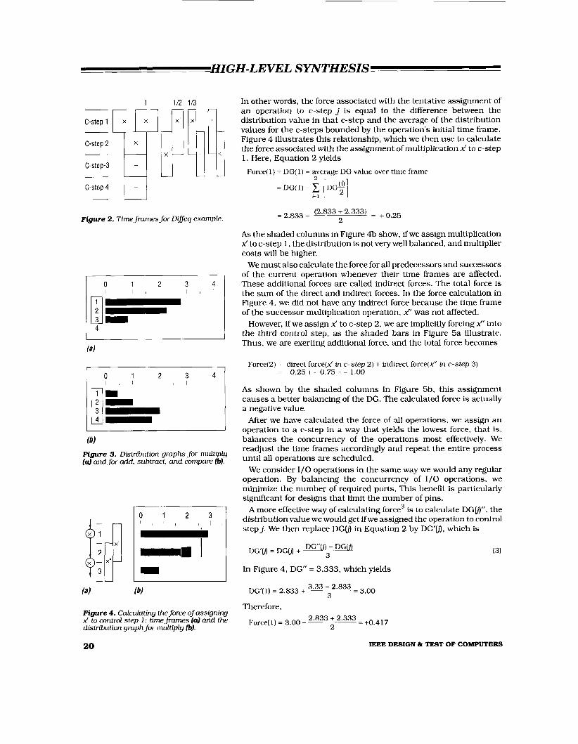
Figure 4. Calculating the force of assigning i to control step 1 : timeframes (4 and the distribution graph for multiply &).

In other words, the force associated with the tentative assignment of an operation to c-step j is equal to the difference between the distribution value in that c-step and the average of the distribution values for the c-steps bounded by the operation’s initial time frame. Figure 4 illustrates this relationship, which we then use to calculate the force associated with the assignment of multiplication A! to c-step 1 . Here, Equation 2 yields

Force( 1) = DG( 1) - average DG value over time frame

= DG(1) - [ D e ] bl

(2.833 + 2.333) = + o.25 2

= 2.833 -

As the shaded columns in Figure 4b show, if we assign multiplication i to c-step 1 , the distribution is not very well balanced, and multiplier costs will be higher.

We must also calculate the force for all predecessors and successors of the current operation whenever their time frames are affected. These additional forces are called indirect forces. The total force is the sum of the direct and indirect forces. In the force calculation in Figure 4, we did not have any indirect force because the time frame of the successor multiplication operation, i‘ was not affected.

However, if we assign i to c-step 2, we are implicitly forcing i’ into the third control step, as the shaded bars in Figure 5a illustrate. Thus, we are exerting additional force, and the total force becomes

Force(2) = direct force(i in c-step 2) + indirect force(d‘ in c-step 3) = - 0.25 + - 0.75 = - 1.00

As shown by the shaded columns in Figure 5b, this assignment causes a better balancing of the DG. The calculated force is actually a negative value.

After we have calculated the force of all operations, we assign an operation to a c-step in a way that yields the lowest force, that is, balances the concurrency of the operations most effectively. We readjust the time frames accordingly and repeat the entire process until all operations are scheduled.

We consider 1 / 0 operations in the same way we would any regular operation. By balancing the concurrency of 1 / 0 operations, we minimize the number of required ports. This benefit is particularly significant for designs that limit the number of pins.

A more effective way of calculating force3 is to calculate DGLj)”, the distribution value we would get ifwe assigned the operation to control step j. We then replace DG(j1 in Equation 2 by DC’bJ, which is

In Figure 4, DG” = 3.333, which yields

3.33 - 2.833 = 3.00 3 DG’( 1) = 2.833 +

Therefore, 2.833 + 2.333 = +o.41,

2 Force( 1) = 3.00 -

20 IEEE DESIGN & TEST OF COMPUTERS

This implements a simple form of lookahead that has considerably improved the force-directed scheduling algorithm's effectiveness.

MINIMIZING STORAGE A N D INTERCONNECTION COST Most scheduling algorithms minimize the cost of functional units

but ignore the associated storage and data-transfer costs, even though scheduling has a direct effect on them. For example, the fewest buses required for a scheduled control-flow or data-flow graph is the number of concurrent data transfers in a control step. The fewest registers required is the maximum number of data arcs that cross the boundary of a control step. Figure 6 illustrates two simple schedules with different hardware costs. The schedule in Figure 6a appears to be the best of the two, since it requires only one multiplier. However, the schedule in Figure 6b may have a lower global cost because the allocation cost for ports and buses and the storage costs are considerably lower.

Minimizing storage costs. The first step in minimizing the number of registers is to create a new class of operations, called storage operations. A storage operation is created at the output of every source operation that transfers a value to one or more destination operations in a later control step. We also need a specid distribution graph, called a storage DG.

We calculate the force of storage operations in much the same way as we do for regular operations. The only complication is that the length, or lifetime, of a storage operation depends on the final schedule. As an example, consider a simple data-flow graph, in which storage operation S has three possible lifetimes. Figure 7a shows the ASAP life, which spans c-steps 2 and 3. In our approach, we combine the ASAP, ALAP, and maximum lifetimes to calculate a nonuniform probability distribution. The sum of the distributions of all the storage operations yields the storage DG shown in Figure 7b. The gray portion of the graph reflects the contribution of S.

We add the storage forces to an operation's direct force by applying a mechanism similar to that used for indirect forces caused by a predecessor or successors.

Minimizing bus costs. To minimize the number of concurrent transfers and the associated bus costs, we create a special distribution graph, called the transfer DG. The transfer DG contains the distributions of the data transfers. Since transfers are directly related to operations, the transfer DG is simply the sum of every operation distribution multiplied by the combined number of distinct inputs and outputs. For example, we have only four distinct inputs and outputs in c-step 2 of Figure 7a. We calculate the forces from these new DGs in the same manner we use for regular operations.

RES0 URCE CONSTRAINTS The force-directed scheduling, or FDS, approach just described

supports the synthesis of data paths that have a near-minimum cost under fixed timing constraints, but does not consider hardware constraints. The FDLS (force-directed list scheduling) approach presented here solves the opposite problem: finding the fastest schedule given fixed hardware constraints. It combines the characteristics and strengths of the well-known list scheduling algorithm* as well as the

DECEMBER 1989

I I I I I I I , 3 1 0 1 2 I -

11n1-a I

Figure 5. Force calculations for ZC scheduled in control step 2: timefiames (4 and the distribution graph for multiply &).

3 Ports

a pJ 2Ports

figure 6. Hardware cost of a schedule requiring one multiplier(4 and two multipliers @J.

21


Forcedirected list scheduling is similar to list scheduling except force is the priority

f indon , not mobility or urgency.

1

Figure 8. List schedule (4 and force- directed schedule &) for a simple example.

(a) fb)

Figure 7. Storage distribution graph.

0 1 2 3 I I I I

FDS algorithm. FDLS uses a global measure of concurrency throughout the scheduling process just as FDS does.

In list scheduling, we sort operations in topological order using control and data dependencies. Ready operations are those we can assign to the first control step. If there are more ready operations of a single type than there are hardware modules to perform them, then we must defer one or more operations. Which operations to defer often depends on some local priority such as mobility or urgency.’ In Figure 8, for example, two add operations may be scheduled in the first control step, so we must defer one of them. Since they are both on the critical path, they have equal mobilities and the same urgency, so we could choose either one. In the figure, the left addition is deferred. We repeat this process, which yields the final schedule requiring four control steps.

FDLS is similar to list scheduling except force is the priority function, not mobility or urgency. Whenever we exceed a hardware constraint during regular scheduling, we calculate the force of the operation to select the best operation(s) to defer. The deferral that produces the lowest force-that is, the lowest global increase of concurrency in the graph-is the best candidate for deferral. We repeat these calculations and the deferral process until we meet the hardware constraint. Typically, the hardware constraint is given as the maximum number of functional units of each type. However, we can apply this principle to data-transfer and storage operations by using fixed limits on buses and registers.

Force calculations depend on the existence of time frames, so we must temporarily specifL some global constraint. In the FDLS algorithm, this constraint is the length of the current critical path. This path gets longer if we have to defer a critical operation to solve a resource conflict.

In Figure 8, the initial time constraint was two control steps. We had to extend it to three control steps immediately to solve a resource conflict between operations on the critical path. The force values in Figure 8b are from the enhanced force formulation given in Equation 3, which has a simple lookahead scheme. In this case, the force values for the two addition operations are not equal. Deferring the


left addition causes a force of +0.5, while deferring the right addition causes only a +0.33 force, so we defer it to c-step 2.

Even for this simple example, FDLS yields a faster schedule than list-scheduling. However, when we take into account the storage and transfer distribution graphs, we could get a different schedule. The final schedule depends the relative values of storage, interconnection, and port costs, as Figure 6 illustrates.

To summarize, the FDLS algorithm, shown in Figure 9, allows us to maintain the advantages of both list scheduling and force-directed scheduling by allowing

high utilization of functional units, as in list scheduling fast computation times, since the FDLS algorithm has a worst case complexity of an2) , where n is the number of operations in the control-/data-flow graph, and typically exhibits linear behavior global evaluation of all the side effects from assigning an operation to a control step, which is a characteristic of force-directed scheduling

SCHEDULING EXAMPLES To illustrate and compare scheduling algorithms, we use the

fifth-order elliptic wave filter described in Kung et al.’s book on signal pro~essing.~ In the first row of Table 1, we summarize the adder and multiplier allocations for timing constraints in FDS. In this table, we assume that multipliers require two control steps for execution, while adders require only one. The minimum timing constraint for this example is 17 c-steps. Using retiming, we could reduce that to 16 c-steps, but to ensure a fair comparison, we do not use retiming. CPU times were between two and six minutes on the Xerox 1108, a Lisp machine with medium to low performance.

The second row of the table is the result of taking the FDS allocations for 17, 19, and 21 c-steps, setting these a s a limit of the number of functional units allowed, and running the FDLS algorithm to get the shortest execution time. For the 17 and 21 c-step allocations, we already had optimal results and so the time could not be reduced. However, for the 19 c-step allocation (two adders and two multipliers), the FDLS algorithm produced a schedule that had one c-step less. This result is optimal with respect to functional unit cost.

Table 1 . Functional unit allocations for diperent execution times: + = adder; x = multiplier, xP= pipelined multiplier: FWS = force-directed schduling, FDLS = force-directed list scheduling, ASAP = as soon as possible, LS = list sc/wduling.

Number of Control Steps 17 18 19 21 Algorithm

FDS +++ xxx +++ xx ++ xx ++ x FDLS +++ xxx ++ xx ++ x

ASAP ++++ xxxx Ls ++ xx

FDS, FDLS +++ xpxp +++xp ++ xp

Initialize time constraint to length of critical path for c-step from 1 to time constraint do:

Determine time frames Determine ready operations in c-step

{operations whose time frame intersects

while (number of ready operations > number of current c-step)

functional units) do if all operations on critical path then

extend time constraint by 1 c-step reevaluate time frames

calculate forces for possible deferrals defer operation with lowest force remove it from ready operations

end; Schedule remaining ready operations in current

c-step end;

Figure 9. The algorithm for force-directed list scheduling.

~~

DECEMBER 1989 23


Regardless of the method choosen, the

designer has an added leuel offlexibility With

this integrated scheduling

methodology.

CPU times were significantly faster than those for FDS, varying between one and two minutes.

One reason for the improved performance of FDLS is that with this algorithm we have more information about the design. We provide the number and type of functional units in FDLS, while FDS uses only a time constraint. FDLS also requires fewer force calculations, which explains the reduced CPU times.

The third row of Table 1 represents the schedule with ASAP scheduling and conditional deferral.5 The fourth row represents the result from CMU's System Architect's Workbench' using list scheduling. Finally, the fifth row shows the HAL results when two-stage pipelined multipliers are used. The use of this type of functional unit involves a simple extension of the force a lg~r i thm.~ Functional unit costs were optimal with both FDS and FDLS. Also, HAL'S register and interconnection costs compare favorably with those from other systems.

A NEW EXPLORATION TECHNIQUE Taken alone, FDLS allows the user to partially spec@ a target

architecture by setting the number and type of functional units, as well as limits on the total register and bus counts. The flexibility of FDLS justifies the small additional effort to implement it.

We have found, however, that the most powerful method of exploring the design space is to use both FDS and FDLS. The designer sets a maximum time constraint and uses the FDS algorithm to arrive at a near-optimal allocation. In this phase, we can take advantage of FDS's ability to automatically perform cost tradeoffs among functional units of different types3

In the second phase, the designer focuses on one area of the design space by using FDLS with the allocation from the first phase to determine if he can get a faster schedule. The faster schedule may be possible because the scheduler starts out with more information about the design.

Regardless of the method choosen, the designer has an added level of flexibility with this integrated scheduling methodology. He can explore the design space from either the area dimension or time dimension. A simple extension of FDS can also solve two types of pipeline scheduling problem^.^ Thus, FDLS combined with FDS provides general algorithms that we can tailor to specific applications. Better still, from the implementer's point of view at least, most subroutines are common to both algorithms.

ALLOCATING DATA PATHS Once we have the schedule and have allocated the functional units,

we need to allocate the data paths. Two of the most important subtasks are allocating registers and interconnections. This empha- sis is justified by McFarland's experien~e,~ which shows that multiplexing costs seem to have the most significant effect on the overall cost-speed tradeoff curve.In HAL, we do this allocation by following three transformation steps:2

1 . Bind operations to functional units. 2. Bind storage operations to registers. 3. Bind data-transfer operations to elements such as multiplexers

and buses.


Bind operations to functional units. We bind all arithmetic and logic operations to specific functional units so as to minimize the number of distinct inputs on each one.

Bind storage operations to registers. We create a storage operation for each data transfer that crosses a c-step boundary. We use a novel technique to divide the variable’s life into two intervals. The first interval lasts one c-step and is assigned to a local storage operation. The remaining c-steps are assigned to the second storage operation. Typically, we assign the two storage operations to the same register. In many cases, however, we could lower the interconnection cost by assigning them to different registers.

Figure 10 illustrates the benefits of local storage. Figure 10a uses regular storage operations and yields the rather complex data path shown in the bottom of the figure. In Figure lob, the local storage operation in c-step 1 is assigned to R1 while the rest of the operation’s life is assigned to R2. The result is a much simpler data path.

Bind data-transfer operations to interconnections. Here, we temporarily bind data transfers to interconnections by creating multiplexers and connecting them to the input of every register and functional unit. We use these multiplexers to form a transfer path to each of their input source objects. We preserve single-input multiplexers because we may want to merge them with other multiplexers to form a bus.

MERGING REGISTERS .

In this important optimization step, we selectively merge registers with disjoint lifetimes. To illustrate the difficulty of this problem, we again refer to the DiffEq example. We determine for each register

.~

1 Q R I

3

m Multiplexer 2

Multiplexer 1 &%2l

1 I Q RI

3

itf Multiplexer 1

Figure 1 0 . Comparison of regular storage (a) and local storage (b).

DECEMBER 1989

Multiplexing costs seem to have the most signijicunt qfect on the overall

cost-speed tradeoflcurve.

25


In this type of partitioning, we reduce the compatibility graph by considering only the registers that have an

interconnection afinity above a certain

threshold.

26

defined the set of disjoint registers. This yields a register-compatibility graph in which each edge represents the disjoint usage times of two registers. These registers are candidates for merging. We could use exhaustive clique partitioning to generate all possible register groupings, but this problem is NP-complete.

Researchers at the University of Southern California' exploit the left-edge algorithm, which yields an optimal track assignment in channel routing. Here, we can apply it to guarantee the minimum number of registers.

Another alternative to exhaustive clique partitioning is heuristic clique partitioning. The Facet system from Carne ie Mellon Uni- versity uses this special form of clique partitioning to determine a near-minimum number of registers. It incorporates heuristics based on the clique graph structure to prune the graph and reduce the number of possible cliques.

Both these approaches, however, ignore the impact of register merging on interconnection costs. An earlier version of HAL2 tried to take interconnection costs into account by merging only registers that were connected to the same functional units, but this technique was not general enough to have much use.

The current version of HAL uses exhaustive clique partitioning but with reduced compatibility graphs, so the problem is no longer NP-complete. This extended version of the earlier HAL register-merging algorithm is called weight-directed clique partitioning. In this type of partitioning, we reduce the compatibility graph by considering only the registers that have an interconnection affinity, or structural weight, above a certain threshold. We progressively lower this threshold as we get fewer compatible pairs after each iteration of the merging routine. We determine the structural weights from the preliminary binding of functional units, multiplexers, and interconnections we performed earlier. The register pairs whose merging gives the lowest interconnection cost are give the highest weight, as Figure 1 1 shows. The weight values of 1 to 4 are for illustration only. The actual values are an estimate of the interconnection area that would

B -

Weight = 4 Weight = 3 Weight = 2 Weight = 1

1

ps

gg D2 D3

Figure 1 1 . Interconnection weights for di@erent register merges before (4 and after (b) the merge.

IEEE DESIGN & TEST OF COMPUTERS

be saved. We evaluate this area using a function that represents the cost of the interconnection area. Thus, weights can be either positive or negative.

If we set the weight threshold high enough, we can limit the complexity of the clique graph at will. For example,.by applying a weight threshold of 4 to the clique graph of Figure 12,-we reduce it to the graph represented by the dotted edges. As we refine the selection of registers for merging, the weight value selected varies with the number of remaining edges in the compatibility graph. This number must be small enough to allow exhaustive (or semiexhaus- tive) clique partitioning in a reasonable time. We then generate all possible merges. For each of these, we evaluate the associated interconnection costs and select the one with the lowest combined register and interconnection cost. For the DiffEq example, the register groups chosen are (R20, R21). (R17. R25). (R16, R23). R18. R19, R22).

We naturally get fewer compatible register pairs with each merge, and we repeat the process until no more merges are possible. In our example, by lowering the threshold to 3, we obtain the final solution which is a clique made up of five register groups:

This is the smallest number of registers possible and-perhaps more important-represents a configuration with a very low interconnection cost.

(R20, R21). (R17. R24, R25). (R16, R23), (R18, R19). R22)

MERGING MULTIPLEXERS A multiplexer is a data-transfer element that has multiple inputs

and a single output. while a bus is an element with multiple inputs and multiple outputs. The problem of merging multiplexers into buses is somewhat the same as the problem of merging registers except that a multiplexer is not used continuously. Thus, a multiplexer created in the method described is assigned to a series of c-steps that are not necessarily contiguous. We cannot use algorithms like the left edge for this reason. We can, however, iise a clique partitioning method similar to what we used for register merging.

Our threshold for merging multiplexers is not interconnection weights, but the number of common inputs between multiplexer pairs. A merge cannot create more than two levels of buses or multiplexers for each transfer path from register to functional unit to register. Thus. we ensure that the dela through the interconnection paths is minimal. SA@ and Splicer allow up to four levels of buses arid multiplexers.

~

fs

DESIGN PARTITIONING The data paths in Figures 13, 14, and 15 show that in addition to

low register and interconnection costs, we have a good structural partitioning of the design. The reason is that we group highly connected elements and so use interconnection information to prune the design space. Although the two merging algorithms we have described are aimed at a general distributed architecture, we can refine them for specific applications. We can introduce different weights to enforce predefmed structural or physical partitions that

DECEMBER 1989

In addition to low register and

interconnection costs, we haue a good

structural partitioning of the design because

wegroup highly connected elements.

- _

- Weight < 4 - - - Weight 2 4

Figure 12. Compatibility graph for the D i E q example in Figure I .

27


I-

Our threshold for merging multiplexers is

not interconnection weights, but the number

of common inputs between multiplexer

pairs.

4 Multiplexer 2/ M u l t i p l e x e r u \ Multiplexer 1/ \ \

t FU2\ (z-) /

Bus 1 I I

Bus 1 I - I I

Bus 3 P Bus4

1 Coeff. ROM I - \ t -

G FU5(>)

\ xp /

Control

I I I I I I I

b

Figure 13. HAL. datapath using nonpipelinedfunctional units.

II I , I V Bus 2

L I I I

l v i - Bus 4 t I

A -

Figure 14 . HAL datapath for D i m using a pipelined multiplier.

l v ! Bus 3 t

1 , , 1

Figure 15. Data path for waveflter example: x p= pipelined multiplier.

I v I


correspond to a specific architecture. Registers (multiplexers) within the same partition would have the highest weight to ensure that they are merged first. By varying the value of the weight, we can experi- ment with compromises in reducing the total number of interconnection lines and preserving the design partitions.

EXPERIMENTAL RESULTS We present two examples to cpmpare our approach with other

systems: the DiffEq differential equation described earlier and a fifth-order waveform elliptic wave which we used earlier to compare scheduling algorithms. We did not fine-tune our algorithm to suit either of these applications. The CPU execution times on a Xerox 1108 are for complete synthesis, including scheduling, allocating functional units, and binding registers and buses.

DIFFERENTIfi EQUATION The DiffEq example, first presented in a paper from the 1986 Design

Automation Conference,2 is used in Splicer8 and Cat~-ee.~ The first four columns of Table 2 are a summary of costs for these systems without pipelined functional units and for the current version of HAL using the register and bus merging algorithms. The results of an earlier version of HAL are given as the baseline for the other systems' percentages. Figure 13 shows the HAL data path using nonpipelined functional units.

In column five of the table, we show results for Splicer with a two-stage, pipelined multiplier. The cost of the functional units in this configuration is consequently much lower. In column six of the table, we show results from HAL when we use force-directed scheduling and weight-directed clique partitioning, as shown in Figure 14.

As the table shows, Splicer and Catree improved on the early HAL'S results, but the current HAL'S register cost is equal to the best result achieved in the other systems, while the interconnection costs are significantly lower.

WAVE FILTER Table 3 compares the HAL designs with those of SAW,' Splicer,'

and Catree.g The table includes the number of multiplexer inputs required-a crude measure of relative interconnection costs. Since HAL also uses buses, this value is actually the combined number of inputs to multiplexers and buses, where we consider a bus the same as a multiplexer with multiple outputs. To help isolate the effects of strategies to allocate registers and interconnections, we compare results with identical time constraints and functional unit allocations.

For all these examples, and with all other costs being equal, the interconnection costs are significantly lower with HAL. Roughly half these savings are the result of using local storage operations, which divide each variable's life into two parts. The total CPU time varies between two and eight minutes.

The bottom row indicates the overall best result from HAL. In this case, HAL uses a two-stage, pipelined multiplier. This design has the lowest interconnection cost of all the examples. The data path for this result is given in Figure 15. The right operand of the pipelined multiplier is a small ROM that contains the filter coefficients.

Our results clearly illustrate the

@ectiveness of using time fi-ames,

distribution graphs, and concurrency

balancing.

DECEMBER 1989 29


We still have issues to address such as the need to incorporate preliminary floor-

planning information into synthesis.

We can make three observations about the data path in the figure.

1. We used six buses, which is relatively few. The connections to and from these buses are mostly local.

2. Because the path from a single register to a functional unit to a register never crosses more than two levels of multiplexers or buses, we reduce the clock-cycle time. Data paths in SAW and Splicer cross up to four levels.

3. As in the DiffEq example, most interconnections are local to the area defined by a single functional unit. The bipartition in SAW is more clearly defined, however, and probably would be easier to lay out.

0 ur algorithms complete two important tasks in high-level synthesis: scheduling under time and resource constraints and allocating buses and registers to minimize interconnection costs. The force-directed scheduling and force-directed

list scheduling algorithms take into account the cost of functional units as well as the cost of storage and interconnections. Also, by combining these algorithms, we have a flexible stepwise refinement approach to exploring the design space. Our results clearly illustrate the effectiveness of using time frames, distribution graphs, and concurrency balancing. This is confirmed by results from systems

Table 2. Summary of area costs for L X i q example.

System HAL86 Splicer Catree HAL89

CPU 40sec N/A N/A 50 sec Intercon- nection (Yo) 100 86 93 79 Register (%) 100 100 83 83 Functional. Unit (Yo) 100 100 100 100

Splicer HAL89 ~~ ~

N/A 120sec

107 84 100 83

64 57

Table 3. Comparison of register and interconnection requirements; + = adder. x = multiplier. 2 = pipelined multiplier.

Number of Number of system Number of Of Multiplexer

Control Steps ~ ~ ‘ & ~ e ~ Registers Inputs

HAL 19 2x, 2+ 12 28 SAW 19 2x, 2+ 12 34 (+2 1YO) HAL 21 lx, 2+ 12 30 Splicer 21 lx, 2+ N/A 35 (+170/) HAL 17 2xp. 3+ 12 31 Catree HAL 19 lXP, 2+ 12 26

17 2xp, 3+ 12 38 (+22%)


that exploit the same principles, as reported at this year’s High-Level Synthesis Workshop.

The approach we have described for allocating registers and buses exploits a simple but powerful weight-directed clique partitioning algorithm based on merging highly interconnected elements. This algorithm prunes the exploration space while favoring merges that reduce interconnection costs.

We still have issues to address such as the need to include floor- planning information in synthesis. We could do this by assigning higher weights to the merging of registers (or buses) in the same floor-plan partition. On the other hand, the whole issue of control costs has gone largely ignored. Although balancing the concurrency of data-path events should reduce the number of control lines, and making the schedule shorter usually reduces the controller size, more accurate metrics for control cost still have to be developed. @3

ACKNOWLEDGMENTS We thank Jenny Midwinter for her insight and advice on interconnection

allocation and Emil Girczyc who helped lay the groundwork for the original FDS algorithm.

This research was funded in part by grants from the National Society of Electronics Research Council of Canada, from Carleton University, and from BNR. Ottawa, as part of a cooperative PhD project.

REFERENCES 1. M. McFarland, A. Parker, and R. Camposano, ‘Tutorial on High-Level Syn-

thesis,” Roc. 25th Design Automation Conf., July 1988, pp. 330-336.

2. P. Paulin, J. Knight, and E. Girczyc, “HAL: A Multi-Paradigm Approach to Automatic Data Path Synthesis,” Roc. Design Automation Conf., July 1986,

3. P. Paulin and J . Knight, “Force-Directed Scheduling for the Behavioral Synthesis ofASICs,” IEEE 7Yans. Computer-Aided Design, Vol. CAD-8, Vol. 6, June 1989, pp. 661-679.

4. S. Davidson et al., “Some Experiments in Local Microcode Compaction for Horizontal Machines,” IEEE Trans. Computers, Vol. C-30, No. 7. July 1981,

5. S. Kung, H. Whitehouse, and T. Kailath, V L S I and Modern Signal Processing, Prentice Hall, Englewood Cliffs, N.J., 1985.

6. D. Thomas et al., ‘The System Architect‘s Workbench,” Proc. Design Automa- tion Conf., July 1988, pp. 337-343.

7. M. McFarland, “Reevaluating the Design Space for Register-Transfer Hard- ware Synthesis.” Proc. Int‘l Conf. Computer-Aided Design, Nov. 1987, pp.

8. B. Pangrle, “Splicer: A Heuristic Approach to Connectivity Binding,” Roc.

9. C. Gebotys and M. Elmasry, * W I Design Synthesis with Testability,” Proc.

pp. 263-270.

pp. 460-477.

262-265.

Design Automation Cont. July 1988, pp. 536-541.

Design Automation Conf.. July 1988, pp. 16-21.

Pierre G. Paulin is a member of the VLSI System Design and Synthesis Department at Bell-Northern Research. Prior to joining BNR full time. he was part of a cooperative research project with Carleton University and BNR to do the work reported in this article. He holds a BSc in engineering physics and an MScA in electrical engineering from Lava1 University and a PhD in electronics from Carleton Uni- versity. He is a member of the IEEE Computer Society.

John P. Knight is an associate professor in the Department of Electronics, Carleton Uni- versity, Ottawa. He holds a BSc from Queen’s University and an MScA and a a PhD from the University of Toronto-all in electrical engineering.

Direct comments or questions on this article to P. Paulin. BNR, PO 35 1 1 , Station C, Ot- tawa, K1Y 4H7. Canada, or to J. Knight, Carleton Univ., Dept. of Electronics, Ottawa, K1S 5B6, Canada.

DECEMBER 1989 31

t the commercial realm, the success

Documents