t-110.5111 computer networks ii - aalto · wlan wcdma watching youtube ... – understand and...
TRANSCRIPT
23.9.2010
T-110.5111 Computer Networks II Energy efficiency 3.12.2012 Matti Siekkinen

Outline
• Motivation • Measuring energy • Modeling energy consumption • Optimizing energy consumption

Which one is Green ICT?
Source: Google image

What is Green ICT?
• Green ICT – Reduce energy consumption of ICT
• What’s involved? – Networked Equipment
• PCs, mobile phones, data centers, set-top boxes,... – Network Equipment (infrastructure)
• Routers, switches, wireless access points, …
Why we give a damn
• ICT energy consumption – About 12% of global power consumption – 60billion KWh wasted by inefficient computing every year – Telecom data volume increases approximately by a factor of 10
every 5 years, which corresponds to an increase of the associated energy consumption of 16-20% every year
• CO2 – At least 2% of global CO2 emission – As much as airplanes, and ¼ of cars
• €€¥££ – Data center and network operators – Large part of operation costs

There’s another dimension to energy consumption • Energy constrained devices
– Smartphones • Need to recharge more and more often
– Sensors and sensor networks • Don’t want to or cannot change batteries often
• Quality of service and availability issue – Not directly about money – Not so much a ”greenness” issue either
• Although scale is very large... • Mobile network infrastructure draws far more power than the
phones
• We focus today mostly on these issues
Some questions worth asking
• How much energy does it cost when you make a phone call, watch YouTube, send an email, or…? – End-to-end
• How much energy is consumed on a network/networked equipment? – In different scenarios – With different workloads
• How much can we reasonably save? – … in network equipment? – ... in networked equipment? – …in different scenarios? – … for different services? – How to do it?
7

Outline
• Motivation • Measuring energy • Modeling energy consumption • Optimizing energy consumption

Power measurement
• System-level power measurement Measure the total power consumption of the whole mobile phone.
• Component-level power measurement
9

Measuring with software
• Simplest way to measure • Nokia Energy Profiler
– Easy to use – Sampling frequency is low (4Hz) – Get accurate information about, e.g.
voltage(V), current(Am) • Measured error just a few % in active cases,
more for low power cases (idle) – Only for Symbian L
10
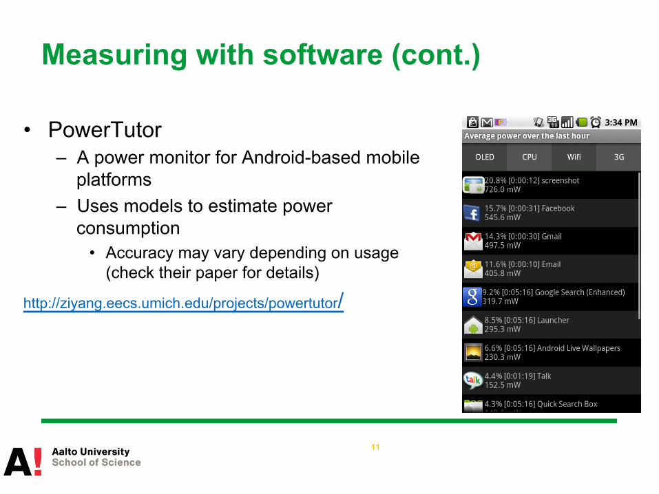
Measuring with software (cont.)
• PowerTutor – A power monitor for Android-based mobile
platforms – Uses models to estimate power
consumption • Accuracy may vary depending on usage
(check their paper for details)
http://ziyang.eecs.umich.edu/projects/powertutor/
11

Glance at the power consumption
12
(5,2.249)
(10,1.281)
(113,1.494)
(211,2.516)
0.000
0.500
1.000
1.500
2.000
2.500
3.000 1
5
10
15
20
25
30
35
40
45
50
55
60
65
70
75
80
85
90
95
10
0
105
11
0
115
12
0
125
13
0
135
14
0
145
15
0
155
16
0
165
17
0
175
18
0
185
19
0
195
20
0
205
21
0
215
22
0
225
23
0
235
24
0
243
24
5
249
Pow
er(W
att)
Time(second)
WLAN WCDMA
Watching YouTube from N95

Using external instruments
13
Power measurement
• System-level power measurement Measure the total power consumption of the whole mobile phone.
• Component-level power measurement
Example: Given a mobile phone, measure the power consumption of each CPU, network interface, and display separately.
14

Component-level power measurement
• Requires information about power distribution network at the circuit level
• Only a few off-the-shelf devices can be measured on component-level – e.g. Openmoko Neo Freerunner – See: Aaron Carroll and Gernot Heiser. An analysis of
power consumption in a smartphone. In Proceedings of the USENIXATC 2010.
15

Outline
• Motivation • Measuring energy • Modeling energy consumption • Optimizing energy consumption

Where does the energy go?
• Hardware consumes the energy
• Amount of energy consumed depends on – Hardware physical
characteristics – Hardware operating mode – Workload generated by
software running on top of hardware
17

Power modeling
• Allows to estimate energy/power consumption even when direct measurement is impossible – Impractical: external instruments usable only in lab settings – Software not available
• Why interesting? – Understand and improve energy consumption behavior of
existing protocols and services • Also in setups which aren’t possible in a lab • Help redesign for better energy efficiency
– Develop energy-aware protocols and applications • Run-time estimation of energy consumption • E.g., choose energy efficient paths, peers, servers
• 18

Power modeling (cont.)
• Power models describe – Transmission cost, computational cost, cooling cost, … – Power consumption of each hardware component or software
component – Power consumption of a service
• Methodology – Deterministic modeling – Statistical modeling
Power measurement is needed for both methods.
19

Example: Transmission energy
• Which one consumes less energy? – 3G, WLAN, or LTE? – Lumia 920 or iPhone 5? – P2P or C/S? – ...
• Not easy questions to answer...
20

Transmission energy metrics
Two metrics • How many Joules are needed for transmitting or
receiving one Bit? – Not constant – Depends on how you send or receive the data – Depends on how you control the operating mode of the network
interface – Poor signal strength requires more transmit power
• How many Bits do you need to transmit or receive? – In bad network conditions, you also need to consider the power
consumed by data retransmission (TCP)
21

Transmission: WNI states and transitions • Managing wireless network interface happens through
states – Set of states are technology specific
• WNI transitions from state to another according to some rules – Usually timer specified transitions
• What states? – E.g. receive, idle, and sleep in WiFi – CELL_DCH, CELL_PCH etc. for 3g
• Correspond to different kind of resource allocation (i.e. channel type)
• States have different power characteristics

Wi-Fi, 3G, LTE: different power states
SLEEP
TRANSMIT
IDLE
RECEIVE PSM
Timeout
Traffic burst
RRC Inactivity timer running
RRC_IDLE
CHAPTER 2. LTE 13
For real-time streaming applications such as voice calls, the data sentduring every transmission and the bandwidth utilized are very small. Forapplications transmitting small amount of data for many times semi persis-tent scheduling is more adaptable in which the UE does not need to requestfor a Grant each time for transmission of data. Instead, the UE is providedwith a transmission pattern which it follows and transmits the data duringthat particular time slot. For example, during a voice call the UE sends aninitial SR and gets the transmission pattern from the scheduler after whichthe data is sent on the allocated time. This reduces the complexities andoverhead of the scheduler and the UE.
There are many di↵erent types of scheduling algorithms which are de-signed based on the need of vendors. Commonly used algorithms includeRound Robin [42], Proportional Fair [47], Maximum Channel Quality Index(CQI) [43], Channel aware scheduling algorithm [42].
2.3 LTE UE and RRC States
In LTE, a UE can shift between three states namely, RRC DISCONNECTED,RRC CONNECTED and RRC IDLE.
Figure 2.4: States of LTE UE
Initially, when the UE is in the OFF state, it does not hold any ac-tive connection with the eNodeB. The state at which the UE is turned onand is searching for a possible base station for registration or the phasewhen the UE is in Airplane mode could be termed as RRC DETACHED

Transmission: Tail energy
• All wireless network interfaces exhibit tail energy – Energy spent being idle with radio on à wasted energy
• Due to inactivity timers – Mandate how long radio is kept listening before state transition
• Timers help with interactive apps and limit signaling – Sporadic communication – Switching radio on and off causes some delay – State transitions require signaling between phone and and base station
• Timer values vary between technology – Wifi≈100ms (can vary) – 3G≈11s (varies between ISPs) – LTE≈10s (varies between ISPs)

How to get rid of tail energy
• Wi-Fi tail is already short • 3G has Fast Dormancy
– Non-standard and standard versions exist – Non-standard will tear down RRC connection: CELL_DCH à
Idle • Problem: frequent use causes a signaling storm
– Standard includes specific signaling msg: CELL_DCH à CELL_PCH
• Less delay to switch back to CELL_DCH and less signaling
• LTE has DRX (discontinuous reception) – 3G has also CPC (continuous packet connectivity) which is
similar (not yet fully supported by networks)

How to get rid of tail energy (cont.) • DRX works in LTE’s connected state
– Hence, also called cDRX (connected mode DRX)
• DRX operates in cycles – Check periodically if new data is waiting – Very similar to PSM in 802.11
2
RRC IDLE.
Fig. 1. States of LTE UE
Initially, when the UE is in the OFF state, it does not holdany active connection with the eNodeB. The state at which theUE is turned on and is searching for a possible base stationfor registration or the phase when the UE is in Airplane modecould be termed as RRC DISCONNECTED state. Once theUE finds base station coverage, it registers to the MobilityManagement Entity (MME) through the LTE Attach proce-dure. After the registration is successful, the UE moves to theRRC CONNECTED state. In the RRC CONNECTED state theUE has a Radio Resource Control (RRC) connection with theeNodeB and maintains an active connection through varioussignaling messages. Once the UE sleeps for a longer durationwithout any data transmission, it moves to the RRC IDLEstate after the expiry of inactivity timer (Inactivity). Whenthe UE is out of coverage area, or during the process ofarea update it de-registers with the eNodeB and moves toRRC DISCONNECTED state.
DRX is the power saving mechanism in LTE, that wasintroduced in order to reduce the power consumption bymaking the UE to move to sleep and idle states when thereis no data transmission to and from the UE based on specifictimers.
In order to obtain information about scheduling, the UserEquipment (UE) monitors the physical down-link controlchannel (PDCCH) information every TTI. Performing thisevery TTI consumes lot of energy as the UE wakes up veryfrequently even though there is no scheduled data for it toreceive. Hence in order to have a solution for overcoming thisissue, Discontinuous Reception (DRX) was introduced. DRXis a proprietary power saving mechanism for LTE, throughwhich the User Equipment (UE) is made to sleep for a longerduration by shutting its wireless RF modem off for a maximumpossible time without compromising the Quality of Service(QoS), latency and user experience. The explanation for DRXin LTE 3GPP was first released with T.36.300, Release 8.
DRX is configured on the UE by Radio Resource Control(RRC) [?], i.e. the eNodeB, which provides the informationon various parameters and its timer values based on which theUE wakes and listens to the PDCCH control information. Themost important part is that, a LTE device can move to DRXstate in both RRC CONNECTED mode and in RRC IDLEmode.
When DRX is deactivated in the network, the UE listens toevery sub frame in the RRC CONNECTED mode. On expiryof inactivity timer, the UE moves to RRC IDLE mode. With
DRX being activated, the transmission and reception of datahappens in the RRC CONNECTED mode. When the UE doesnot receive any data for a certain time, it enters the DRX cyclephase and activates the Short DRX cycle with Short DRXtimer (Ts). In the Short DRX cycle state, the UE monitors thePDCCH during the DRX OnTimer period.
Fig. 2. RRC State transition of LTE UE
The Short DRX timer is active for a time period called asthe Short DRX timer period (TS)after which the UE activatesthe Long DRX timer (Tl). In Long DRX cycle, the wakeupduration of the UE for monitoring the PDCCH is less frequentthan the Short DRX cycle. Once the UE enters the Long DRXcycle, it shifts from the RRC CONNECTED to RRC IDLEmode if the Inactivity timer expires. When the UE gets anintimation about data to be received through the PDCCH, orwhen it needs to transmit data, it moves from RRC IDLEmode to RRC CONNECTED mode. Once all the data istransmitted, the UE again activates the DRX cycle in theRRC CONNECTED mode and then moves to the RRC IDLEmode after inactivity timer expiry.
Fig. 3. LTE DRX
A. OnDuration Timer
On Duration, is the time period an UE is awake for listeningto the PDCCH frame that specifies whether it has any down-link data transfer to happen. It happens during the start of aDRX Long cycle, DRX Short cycle and spans the durationspecified for the timer. After the end of OnDuration, the UEgoes to the sleep mode if there is no DL data assignment ortriggers the inactivity timer if it has a DL data assignment inthe near future.
arriving data
DRX inactivity timer (DRXidle)
DRX cycle (DRXc)
RRC inactivity timer (Tidle)
CONNECTED STATE IDLE STATE Rx on
Rx off transition
to Idle DRX on-duration
timer (DRXon)

Case study 1: Deterministic modeling
Power modeling of data transmission over 802.11g
• Xiao, Y., Savolainen, P., Karppanen, A., Siekkinen, M., and Ylä-Jääski, A. Practical power modeling of data transmission over 802.11g for wireless applications. In Proceedings of the e-Energy 2010.
27

Power consumption of 802.11 wireless network interface (WNI)
• Power consumption depends on operating mode Energy = Power(operating mode)* Duration(operating mode)
28
Continuously Active Mode (CAM)
Power Saving Mode(PSM)
IDLE
TRANSMIT RECEIVE
SLEEP PS
TRANSMIT PT
IDLE PI
RECEIVE PR
PSM Timeout
Tsleep = TI - Ttimeout

WNI operating modes and power
• Order of magnitude less power drawn in sleep state
WNI operating mode Average Power (W)
Nokia N810 HTC G1 Nokia N95
IDLE 0.884 0.650 1.038
SLEEP 0.042 0.068 0.088
TRANSMIT 1.258 1.097 1.687
RECEIVE 1.181 0.900 1.585

Operating modes and traffic patterns
• Problem: No common open API for querying the current operating mode
• Idea: Estimate the operating modes & durations from observed traffic patterns – Take into account 802.11 Power Saving Mode(PSM)
Figure: I/O graph of YouTube traffic (Byte/tick)

Per-burst computation
• TCP style bursty traffic naturally fits to this model • Reduce computational work
– If CBR -> use 1 pkt bursts • Definitions
– Burst: Pkt interval < t • t is a predefined threshold
– Burst size SB – Bin rate r = SB/T = SB/(TB+TI)
• 31
Burst Duration TB
Burst Interval TI
Packet Interval

Taking PSM into account
• PSM timeout effect (the tail energy!) – When Tsleep = 0 – Threshold bin rate rc = SB/ (TB+ Ttimeout)
• Scenario 1: {{r >= rc } and {PSM is enabled}} or {PSM is not enabled} – No time to sleep in between bursts – Alternate between Rx/Tx and idle
• Scenario 2: { r < rc } and {PSM is enabled} – Manage to enter sleep state in between bursts
32

Downlink Power Consumption
33
TB
TI
Power(W)
Ps
PI
PR
PT
SLEEP IDLE RECEIVE TRANSMIT
Energy(J): E = PRTB+ PITI
Power(W): Pd(r) = E/T
Energy Utility (b/J): E0(r) = r/Pd(r)
TCP ACK transmission happens in between receiving packets of data burst à can be ignored in the model

Downlink Power Consumption
• Scenario 1 E = PRTB+ PITI
Pd(r) = E/T = PI + r(PR – PI) TB/SB
• Scenario 2 E = PRTB+ PITtimeout + PSTsleep
Pd(r) = E/T =PS + r[(PR – PS) TB/SB+ (PI – PS) Ttimeout/SB]
Time
PR
PI
TB TB+ TI
Power
Time
PR
PI
TB TB+ TI
Power
TB+ TI+ Tsleep

TCP Power Consumption
Downlink data rate rd Downlink burst size SB
Uplink data rate ru = nSACKrd/SB Data rate threshold rc = SB/(Td+Tu+Ttimeout) Scenario 1: P(rd)=Pd(rd)+Pu(ru)-PI= PI+[Td(PR-PI)+Tu(PT-PI)]rd/SB Secenario 2: P(rd)=Pd(rd)+Pu(ru)-PS =PS+[Td(PR-PS)+Tu(PT-PS)+Ttimeout(PI-PS)]rd/SB
35
n ACKs
n packets
Td Tu

Validation
• Experimental Setup
36
802.11g Access Point
Tested Device
Linux Server
R
DC Power Supply
Multimeter
PC
Data
TCP Server(netcat)
Traffic Shaper(Trickle)
Network Monitoring(Wireshark)

Internet flow characteristics
37
N o k i a N810
HTC G1 Nokia N95
Downlink burst size (KB) 4 4 4
Downlink burst duration (ms) 8 10 10 Uplink burst duration (ms) 0.5 0.5 0.35
N o k i a N810
HTC G1 N o k i a N95
Uplink burst size (KB) 4 4 4 Uplink burst duration (ms) 6 8 12 Downlink burst duration (ms) 0.1 0.1 0.2
0.0 0.1 0.2 0.3 0.4 0.5 0.6 0.7 0.8 0.9 1.0
0 30 60 90 120 150 180 210 240 270 300
Prob
abili
ty
Packet Interval (ms)

Nokia N810: power vs. throughput
38
0.0 0.2 0.4 0.6 0.8 1.0 1.2
0 32 64 96 128 160 192 224 256
Avg
Pow
er(W
)
Data rate limit(KB/s)
Download, CAM
Measured
Estimated 0.0 0.2 0.4 0.6 0.8 1.0 1.2
0 32 64 96 128 160 192 224 256
Avg
Pow
er(W
)
Data rate limit(KB/s)
Download, PSM
Measured
Estimated
0.0 0.2 0.4 0.6 0.8 1.0 1.2
0 32 64 96 128 160 192 224 256
Avg
Pow
er(W
)
Data rate limit(KB/s)
Upload, CAM
Measured Estimated 0.0
0.2 0.4 0.6 0.8 1.0 1.2
0 32 64 96 128 160 192 224 256
Avg
Pow
er(W
)
Data rate limit(KB/s)
Upload, PSM
Measured Estimated
Q: What’s this?
A: Effect of (adaptive, i.e. with a timeout) PSM: manage to catch sleep in between packets/bursts when rate is low enough
When rate ≥ 64KB/s, PSM has no effect!
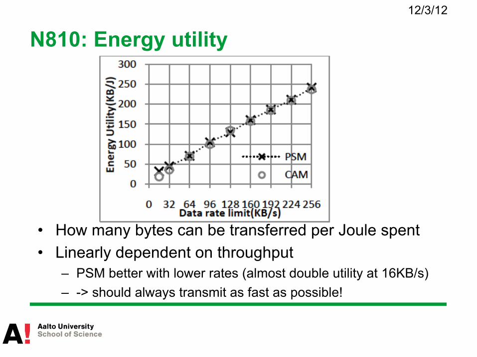
N810: Energy utility
• How many bytes can be transferred per Joule spent • Linearly dependent on throughput
– PSM better with lower rates (almost double utility at 16KB/s) – -> should always transmit as fast as possible!
12/3/12

Accuracy and limitations
Downloads: MAPE less than 7%
Uploads: MAPE less than 6%
0.0
0.2
0.4
0.6
0.8
1.0
0 0.05 0.1 0.15 0.2 0.25 0.3 0.35
F(M
APE
)
MAPE
0.0
0.2
0.4
0.6
0.8
1.0
0 0.1 0.2 0.3 0.4 0.5
F(M
APE
)
MAPE
q Also tried run time estimation § YouTube download through public
AP § MAPE about 11%
§ Most likely due to additional e.g. broadcast traffic
q Limitations § Model does not “see” L2 traffic
o Has an effect on power consumption
§ Model does not separately consider computation caused by packet processing
o Implicitly included in baseline measurements
Case study 2: statistical modeling
System-level power modeling on mobile devices
– Y. Xiao, R. Bhaumik, Z. Yang, M. Siekkinen, P. Savolainen, and A. Ylä-Jääski. A System-level Model for Runtime Power Estimation on Mobile Devices. In Proceedings of GreenCom 2010.
– Similar methodology used in other related work as well • E.g. server processor power modeling
12/3/12

Overview
• A system-level power model – Include main components
• Processors, wireless network interfaces, display – Build using system-level measurements
• Difficult to measure components separately – Generic model
• Not tied to specific application
• Statistical modeling using linear regression – Impossible to track exactly what happens e.g. within CPU – Cannot apply deterministic method
42

Linear Regression with Nonnegative Coefficients
• Linear regression widely used for processor power modeling – Build a linear relationship between the p predictor variables and power
consumption based on n observations
– Need to train the model beforehand!
• Hardware performance counters (HPC) as variables – Set of special registers in modern CPUs – Counters about hardware-related activities – E.g. #cycles, cache activities
∑ =+= p
1j jijj0i xgyf )()( ,ββ
predictor variables
variable coefficients preprocessing function
intercept

Linear Regression with Nonnegative Coefficients (cont.) • Mobile devices can only monitor a subset of HPCs at a
time – E.g., 3 out of 17 HPCs in Nokia N810 – Solution: reduce the set of HPCs using nonnegative coefficients
constraint • Coefficient indicates that variable’s contribution to power -> Select only three variables with highest coefficients • Requires reasonable assumption: increasing activity (HPC value)
never implies reduction in power draw
• Network and display also consume power – Must include them into the model

Regression variables
• Target: reflect resource consumption of a mobile application • Local computing
– 17 HPC-based event rates • CPU activity, memory access
• Network I/O – Download data rate – Upload data rate – CAM switch
• Effect of 802.11 power saving mechanism
• Display – Brightness level

Benchmarks and data collection
• Collect data from test cases for model fitting and evaluation • Goals:
– Stress all selected variables – Explore the space of their cross product
• Nokia Internet Tablet N810 – Only 3 HPCs monitored at a time -> Need to run many iterations to cover all 17 HPCs
• Different categories of workloads: – Idle with different brightness levels – Audio/video players/recorders – File download/upload at different (limited) transfer rates – Audio/video streaming
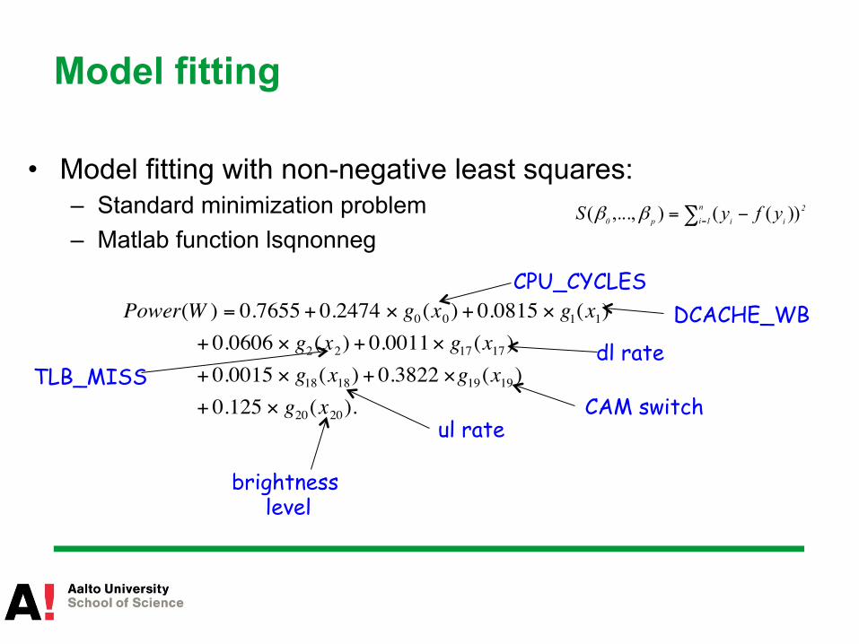
Model fitting
• Model fitting with non-negative least squares: – Standard minimization problem – Matlab function lsqnonneg
∑ = −= n
1i2
iip0 yfyS ))((),...,( ββ
€
Power(W ) = 0.7655 + 0.2474 × g0(x0) + 0.0815 × g1(x1)+ 0.0606 × g2(x2) + 0.0011× g17(x17)+ 0.0015 × g18(x18) + 0.3822 ×g19(x19)+ 0.125 × g20(x20).
CPU_CYCLES DCACHE_WB
TLB_MISS dl rate
ul rate CAM switch
brightness level

Model evaluation
• Evaluation based on similar data used for model fitting – But not the same!
• Similar (or even better) results with another independent data set – Different set of applications
48
4.8
2.0 3.7
0.2
13.7
3.8
0.8
0 2 4 6 8
10 12 14
Radio LiveTV YouTube Audio recorder
Video recorder
upload download
Median Error(%)
Outline
• Motivation • Measuring energy • Modeling energy consumption • Optimizing energy consumption

How to save energy?
• Switch off unnecessary hardware
• Reduce the Joule per Bit, per Cycle, per instruction
• Reduce the workload – Amount of bytes to transmit – Number of instructions to execute
50

Switch off unnecessary hardware Not working = Zero Watt
• What can be turned off?
• When can it be turned off?
• How to leverage the difference in power consumption among the operating modes?
51
Example 1: Sleeping
• Save network equipment (i.e. routers) energy – PSM equivalent for WLAN clients
• Observation 1: Networks are provisioned for peak load – Average utilization remains relatively low
• Observation 2: Routers and switches are usually far from energy proportional – Roughly the same power draw with any load
• Idea: turn (parts of) lightly loaded routers off occasionally – Power draw is somewhat proportional to nb of active ports – Switch off some routers and route traffic around
12/3/12
Sleeping routers
• Time driven sleeping – If router sleeps when packets arrive -> packet loss
• Need to carefully consider when a link can sleep
• Wake on arrival – Link sleeps when idle, awakes upon arriving packet, goes back
to sleep – Require specific technology
• Not currently implemented in OTS routers • Some implications on network mgmt
– How to know if a router is sleeping or if it has crashed? • These mechanisms are currently on research level
– Not commercially deployed (AFAIK)
12/3/12

Example 2: Wake-on-LAN
• Reduce the energy consumption of networked equipment – E.g. workstations within an enterprise network
• Go to sleep while idle • Q: When to wake up? • A: Proxy sends a “magic” packet that triggers wake-
up – Some part of NIC must remain powered up – Requires explicit support from the NIC
• Optimize further: Proxy handles some traffic on behalf of sleeping host – No need to wake up host for each request – Proxy replies on behalf of the sleeping host
• Wake-on-Wireless-LAN also exists
• 54

Reducing per-unit power consumption • Low-power hardware
– Necessary especially in longer term – We take advantage of these but we’ll ignore here on how they
are designed and built
• Power management of hardware devices – DVFS, PSM – Important that protocols leverage these properly!
55

Example 3: Dynamic voltage and frequency scaling (DVFS) • Dynamic power(switching power) of microprocessor
C·V2·f, – C=capacitance being switched per clock cycle, V=voltage, and
f=switching frequency • DVFS
– Adjust the CPU frequency level on-the-fly based on workload – Reduce dynamic power – Reduce the cooling cost (generate less heat)
• Both voltage and frequency usually adjusted simultaneously – Combination is called P-state
• Several implementations exist – AMD: PowerNow!, Cool’n’Quiet – Intel’s SpeedStep
• 56

Dynamic Modulation Scaling (DMS)
• Reduce communication energy per bit
• Trade-off between energy and performance – Similar principle than in DVFS
• Change modulation dynamically – Slows down transmission in a certain
rate instead of operating a MAX rate and going to sleep during IDLE
57
Energy delay tradeoff of QAM (b is nb if bits per symbol)

Dynamic resource scaling
• In general, two opposing approaches exist – “Race to idle/sleep”
• Idea is to use all available resources when have work to do • Sleep rest of the time, i.e. get to sleep as fast as possible
– Scaling proportionally • Scale resource consumption all the time
• Example: multimedia streaming – Race to sleep: transmit data in bursts, sleep in between – Scaling: transmit CBR traffic and adjust modulation to match the
stream rate
12/3/12

Example 4: Traffic shaping
• Mobile media streaming drains battery quickly – Constant bit rate multimedia traffic is not energy friendly – Forces the network interface to be active all the time
• Idea: Shape traffic into bursts so that it is more energy efficient to receive – Remember the linear relationship with throughput – “Race to sleep”
12/3/12
Datarate (kBps)
Start-up Time (s)
WLAN power (W) 3G power (W)
PSM CAM 48kBps 2Mbps
8 18 0.53 1.06 1.30 1.30 16 10 0.99 1.07 1.30 1.30 24 10 1.04 1.07 1.27 1.35
Mobile Internet Radio power draw on E-71 (TCP-based streaming)

Traffic Shaping with Proxy
• Client sends request to proxy • Proxy
– forwards request to radio server – receives and buffers media stream – repeatedly sends in a single burst to client
• 802.11 – PSM is enabled – WNI wakes up to receive a burst at a time – Waste only one timeout per burst
• 3G & LTE – Long enough burst interval à inactivity timers expire à switch to lower power state or activate DRX in
between bursts
60

What is the right burst size?
• Use as large as burst size as possible – Maximize sleep time in between bursts
• Burst size that offer maximal energy savings exists – Option 1: Due to limited buffer size at mobile device
• Max burst size = playback buffer size+TCP receive buffer size • Larger burst will be received at stream rate à lower energy utility
– Option 2: Max burst interval & size limited by amount of initially buffered content
• Cannot let the playback buffer run dry

What is the right burst size?
• Use as large as burst size as possible – Maximize sleep time in between bursts
• Burst size that offer maximal energy savings exists – Option 1: Due to limited buffer size at
mobile device • Max burst size = playback buffer size
+TCP receive buffer size • Larger burst will be received at stream
rate à lower energy utility – Option 2: Max burst interval & size
limited by amount of initially buffered content
• Cannot let the playback buffer run dry

How much energy can be saved?
• Wi-Fi: 65% for audio streaming, 20% for video streaming • 3G: 36% for audio streaming, 30% for video streaming • LTE: 60% for audio streaming, 55% for video streaming
App / Network type Samsung Nexus S (Android, 3G)
Nokia N900 (Maemo, 3G)
Nokia E-71 (Symbian, 3G)
HTC Velocity (Android, LTE)
Internet Radio/Wi-Fi 23%–128–14 s 62%–128–14 s 65%–128–6 s –
Internet Radio/3G/LTE 36%–128–14 s 34%–128–14 s 2%–128–4 s 60%–128–18 s
YouTube Bro/Wi-Fi 14%–912–36 s 20%–328 –39 s 18%–280–4 s –
YouTube Bro/3G/LTE 20%–328–38 s 24%–328–39 s 4%–280–3 s 50%-2000-31 s
YouTube App/ Wi-Fi 13%–458–39 s – – –
YouTube App/3G/LTE 27%–458–39 s – – 54%–2000–39 s
Dailymotion/Wi-Fi 15%–452–33 s – – –
Dailymotion/3G/LTE 30%–452–33 s – – 55%–452–33 s
cell info: energy savings(%)–stream rate (kbps)–optimal burst interval
How much energy can be saved? (cont.)
• Savings depends largely on network type – 3G has long inactivity timers and no discontinuous reception
(yet)
• Network parameters have also a large impact – They determine the tail energy that can be saved
• Stream rate matters as well – Bursting lower rate stream yields larger savings
• Smaller savings with video streaming compared to audio – Display draws significant amount of power – Video decoding is more work than audio decoding

How to save energy?
• Can we just turn off unnecessary hardware?
• Can we reduce the Joule per Bit, per Cycle, per instruction?
• Can we reduce the workload (e.g traffic size)?
65

How can we reduce the workload?
• Getting by with less traffic – Clever transport protocols – Smart application design
• Doing less computation – Offload the work
• Trading transmission to computation
66

Example 5: Data compression
• Communication energy consumption ~ Traffic size • Compression can reduce amount of traffic generated
– But computation costs also energy
• Tradeoff always exists Communications
cost (reduced traffic size)
Computational cost
(compression, decompression)

Compression vs. communication
• Compress ratio differs between data type – Same work but varying savings in bytes
• Must make decision beforehand whether compression would be beneficial – Should we spend energy trying to compress or not? – Must compare communication energy savings (compress ratio)
and energy to compress/decompress – Use model based estimates
• Compression Effectiveness: ce

Evaluation (mobile E-mail)
69
File Extension/Type
With compression Without Compression ce
Energy (J)
Duration (s)
Energy (J)
Duration (s)
.doc 9.61 7.0 18.31 11.8 6.90
.bmp 5.86 5.4 15.74 9.7 2.67
.pdf 25.55 22.8 28.45 23.0 1.03
.txt 13.80 12.2 18.97 13.0 2.68 Binary data 12.8 11 17.57 11.8 2.68
10~ 60% energy savings with N810

Example 6: Computation offloading
• Execute parts of program on remote server • Leverage same tradeoff as with previous example
– Transferring required state to server and back consumes energy – But we save computation energy
• Dynamic decision making – Figure out on the fly which parts of program are worth offloading – Need accurate models for communication and computation
energy consumption • Several proposed frameworks exist
– MAUI, CloneCloud – Research prototypes
70

MAUI • Microsoft’s Requires source code • Using MAUI
– Build app as a standalone phone app – Add .NET attributes to indicate “remoteable” methods
12/3/12
Maui server Smartphone
Application
Client Proxy
Profiler
Solver
Maui Run(me
Server Proxy
Profiler
Solver
Maui Run(me
Application
RPC
RPC
Maui Controller
E. Cuervo, A. Balasubramanian, D. Cho, A. Wolman, S. Saroiu, R. Chandra, and P. Bahl, MAUI: Making Smartphones Last Longer with Code Offload, in MobiSys 2010

CloneCloud
• Intel’s CloneCloud offloads Android program code • Works directly on bytecode
– No need for source code • Modified Dalvik VM • Dynamic thread migration between phone and cloud
12/3/12
Byung-Gon Chun and Petros Maniatis. Augmented Smart Phone Applications Through Clone Cloud Execution. Proceedings of HotOS XII, 2009.

What else could be done?
• Data centers – Liquid cooling for servers, use the hot water to heat other
premises – Run servers in (freezing) cold areas – Renewable energy – Execute things where energy is cheap
• Mobile devices – Smarter (cooperative) scheduling to reduce contention – Leverage alternative low-power radios (e.g. Zi-Fi or Blue-Fi) – Energy harvesting
• Kinetic, solar, ambient radiation, … – Detect and quarantine energy bugs
• Check out Carat (http://carat.cs.berkeley.edu)
73

Summary
• Energy efficiency is a hot topic for several reasons – Saving energy means saving money and saving the planet J – Battery operated devices benefit from energy efficient protocols
• Measuring and modeling energy consumption necessary – Understand how energy is consumed – Improve energy efficiency of protocols and apps – Develop energy aware protocols and apps
• Several ways to save energy – Switch off hardware dynamically – Reduce joules per bit, per cycle, per instruction
• Low-power hardware & smart power management – Reduce workload
• Trade some computation to communication

Additional reading
• Mohammad Ashraful Hoque, Matti Siekkinen, Jukka K. Nurminen. Energy Efficient Multimedia Streaming to Mobile Devices - A Survey. Accepted for IEEE Communications Surveys and Tutorials. 2012.
• Barr, K. C. and Asanović, K.,"Energy-aware lossless data compression," ACM Trans. Comput. Syst. vol. 24, no. 3, pp. 250-291. August 2006.
• Byung-Gon Chun, Sunghwan Ihm, Petros Maniatis, Mayur Naik, and Ashwin Patti. CloneCloud: elastic execution between mobile device and cloud. In ACM EuroSys 2011.
• Aki Saarinen, Matti Siekkinen, Yu Xiao, Jukka Nurminen, Matti Kemppainen and Pan Hui. Can Offloading Save Energy For Popular Apps?. In ACM MobiArch 2012.
• Mikko Pervilä and Jussi Kangasharju. Running servers around zero degrees. In Green Networking 2010.
• Asfandyar Qureshi, Rick Weber, Hari Balakrishnan, John Guttag, and Bruce Maggs. 2009. Cutting the electric bill for internet-scale systems. In ACM SIGCOMM 2009.
75