system level simulations for cellular networks using matlab · system level simulations for...
TRANSCRIPT

System Level Simulations for Cellular Networks Using MATLAB
Sriram N. Kizhakkemadam, Swapnil Vinod Khachane, Sai Chaitanya Mantripragada
Samsung R&D Institute Bangalore
1

Cellular Systems
Cellular Network: A wireless communication network that ideally provides ubiquitous voice & data service
Deployment: Base stations (BS) of varied transmit power levels are installed on a terrain Receivers of users (UE) decode signals from “attached” Base Stations
Challenge: Terrain and propagation effects significantly affect performance Solution: Schemes that mitigate challenge have to be evaluated using Link & System Level
Simulations before deployment
2 Fig. courtesy of : 4GAmericas

System Level Simulation Process
Deployment System configuration
Move UE’s: Pre-Defined Mobility Pattern
Link Establishment (BS-UE Association)
Channel Generation (LoS/NLoS Channel)
Receive Processing Feedback Report
Measurement & Processing Handover Execution
Metrics (Throughput & Handover)
Scheduler (PF / RR)
3
Basic modules
Throughput Modules
Mobility Modules
4
18
1
2
3
4
5
6
7
8
9
10
11
12
13
14
15
16
17
[1]
[0]
[2]
[3]
[4] [5]
Uniform DroppingDiscard region
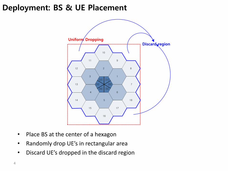
Deployment: BS & UE Placement
• Place BS at the center of a hexagon
• Randomly drop UE’s in rectangular area
• Discard UE’s dropped in the discard region

5
18
1
2
3
4
5
6
7
8
9
10
11
12
13
14
15
16
17
[1]
[0]
[2]
18
1
2
3
4
5
6
7
8
9
10
11
12
13
14
15
16
17
18
1
2
3
4
5
6
7
8
9
10
11
12
13
14
15
16
17
18
1
2
3
4
5
6
7
8
9
10
11
12
13
14
15
16
1718
1
2
3
4
5
6
7
8
9
10
11
12
13
14
15
16
17
18
1
2
3
4
5
6
7
8
9
10
11
12
13
14
15
16
17
18
1
2
3
4
5
6
7
8
9
10
11
12
13
14
15
16
17
[3]
[4] [5]
Link Establishment: Single Tier Case (1/5)
• Find Nearest Cell to a UE using wrap around model • Wrap around model ensures correct mapping of distance from UE to all Base Stations

• Find the set of neighboring 19cells for each UE according to the wrap around model
6
18
1
2
3
4
5
6
7
8
9
10
11
12
13
14
15
16
17
[1]
[0]
[2]
18
1
2
3
4
5
6
7
8
9
10
11
12
13
14
15
16
17
18
1
2
3
4
5
6
7
8
9
10
11
12
13
14
15
16
17
18
1
2
3
4
5
6
7
8
9
10
11
12
13
14
15
16
1718
1
2
3
4
5
6
7
8
9
10
11
12
13
14
15
16
17
18
1
2
3
4
5
6
7
8
9
10
11
12
13
14
15
16
17
18
1
2
3
4
5
6
7
8
9
10
11
12
13
14
15
16
17
[3]
[4] [5]
Link Establishment: Single Tier Case (2/5)

Calculate path loss and shadow from neighboring 19 cells 3 sector
7
18
1
2
3
4
5
6
7
8
9
10
11
12
13
14
15
16
17
[1]
[0]
[2]
18
1
2
3
4
5
6
7
8
9
10
11
12
13
14
15
16
17
18
1
2
3
4
5
6
7
8
9
10
11
12
13
14
15
16
17
18
1
2
3
4
5
6
7
8
9
10
11
12
13
14
15
16
1718
1
2
3
4
5
6
7
8
9
10
11
12
13
14
15
16
17
18
1
2
3
4
5
6
7
8
9
10
11
12
13
14
15
16
17
18
1
2
3
4
5
6
7
8
9
10
11
12
13
14
15
16
17
[3]
[4] [5]
Path loss calculation including shadow effect
Link Establishment: Single Tier Case (3/5)

• Find serving cell and sector : Lowest path loss including shadow effect
8
18
1
2
3
4
5
6
7
8
9
10
11
12
13
14
15
16
17
[1]
[0]
[2]
18
1
2
3
4
5
6
7
8
9
10
11
12
13
14
15
16
17
18
1
2
3
4
5
6
7
8
9
10
11
12
13
14
15
16
17
18
1
2
3
4
5
6
7
8
9
10
11
12
13
14
15
16
1718
1
2
3
4
5
6
7
8
9
10
11
12
13
14
15
16
17
18
1
2
3
4
5
6
7
8
9
10
11
12
13
14
15
16
17
18
1
2
3
4
5
6
7
8
9
10
11
12
13
14
15
16
17
[3]
[4] [5]
Serving Cell/Sector
Link Establishment: Single Tier Case (4/5)

• Identify interferers from 19 cells
9
18
1
2
3
4
5
6
7
8
9
10
11
12
13
14
15
16
17
[1]
[0]
[2]
18
1
2
3
4
5
6
7
8
9
10
11
12
13
14
15
16
17
18
1
2
3
4
5
6
7
8
9
10
11
12
13
14
15
16
17
18
1
2
3
4
5
6
7
8
9
10
11
12
13
14
15
16
1718
1
2
3
4
5
6
7
8
9
10
11
12
13
14
15
16
17
18
1
2
3
4
5
6
7
8
9
10
11
12
13
14
15
16
17
18
1
2
3
4
5
6
7
8
9
10
11
12
13
14
15
16
17
[3]
[4] [5]
Serving Cell/Sector
Interferers
Link Establishment: Single Tier Case (5/5)

Design of Parameters for Deployment
BS & Pico Deployment
• Inter BS/Pico Distance and Number of Picos/Sector, UE’s/Sector
• Transmit Power Levels and Antenna patterns
Fading
•Large Scale Fading: Line of Sight (LOS), Non-Line of Sight (NLOS)
•Shadow Fading
•Small Scale Fading Models
Coverage Maps
•SINR Profile
•Throughput Profile
Mobility
•Handover Parameters
•UE Mobility Pattern
Data Traffic
•Full Buffer
•Partial Buffer: Arrival Rates
Resource Allocation
•Choice of Scheduler Algorithm and Granularity of Allocation
•Transmission Modes: Single, Multiple, Coordinated Transmission
Metrics
•Throughput
•Mobility
• Iterative • Time Consuming
10

Design of Parameters Using Symbolic Math Toolbox
Fig. Deployment of Base Stations and Users according to a Poisson Point Process Model (PPP)
Fig. Deployment of Base Stations by a major cellular network provider in 40 X 40 Km area.
PPP model accurately models the large scale SINR for several practical deployment scenarios
Figs. obtained from: “A Tractable Approach to Coverage and Rate in Cellular Networks,” J. G. Andrews, F. Baccelli, and R. K. Ganti Ergodic Rate as given in, “Modeling, Analysis and Design for Carrier Aggregation in Heterogeneous Cellular Networks,” X. Lin, J.G. Andrews and A. Ghosh
Integral of Hypergeometric Function Evaluated Using Symbolic Math Toolbox
Obtain Density of BS for required Throughput
11

Design of Deployment Parameters Using Symbolic Math Toolbox
BS & Pico Deployment
•Inter BS/Pico Distance and Number of Picos/Sector, UE’s/Sector
•Transmit Power Levels and Antenna patterns
Fading
•Large Scale Fading: Line of Sight (LOS), Non-Line of Sight (NLOS)
•Shadow Fading
•Small Scale Fading Models
Coverage Maps
•SINR Profile
•Throughput Profile
Mobility
•Handover Parameters
•UE Mobility Pattern
Data Traffic
•Full Buffer
•Partial Buffer: Arrival Rates
Resource Allocation
•Choice of Scheduler Algorithm and Granularity of Allocation
•Transmission Modes: Single, Multiple, Coordinated Transmission
Metrics
•Throughput
•Mobility
• Fewer Iterations
Parameters Designed Using PPP Model and Symbolic Math Toolbox
12
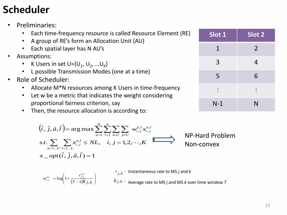
Scheduler
Slot 1 Slot 2
1 2
3 4
5 6
: :
N-1 N
• Preliminaries: • Each time-frequency resource is called Resource Element (RE) • A group of RE’s form an Allocation Unit (AU) • Each spatial layer has N AU’s
• Assumptions: • K Users in set U={U1, U2, …UK} • L possible Transmission Modes (one at a time)
• Role of Scheduler: • Allocate M*N resources among K Users in time-frequency • Let w be a metric that indicates the weight considering
proportional fairness criterion, say • Then, the resource allocation is according to:
1)ˆ,ˆ,ˆ,ˆ(_
,,2,1,,..
maxargˆ,ˆ,ˆ,ˆ
...1 ...1
,
,
,
,
1 1
,
,
lajioptx
KjiNLxts
xwlaji
Ua Ll
la
ji
la
ji
N
a
L
l Ui Uj
la
ji
NP-Hard Problem Non-convex
kjRT
rw
la
kjla
ji
,11log
,
,,
,
kj
r, Instantaneous rate to MS j and k
kjR , Average rate to MS j and MS k over time window T
13

Scheduler: Numerical Solution Using MATLAB
1)ˆ,ˆ,ˆ,ˆ(_
,,2,1,,..
maxargˆ,ˆ,ˆ,ˆ
...1 ...1
,
,
,
,
1 1
,
,
lajioptx
KjiNLxts
xwlaji
Ua Ll
la
ji
la
ji
N
a
L
l Ui Uj
la
ji
• Use MATLAB’s Compiler Runtime Engine
• Solve using MATLAB’s Optimization Toolbox: • Use Binary Integer Programming to Solve the problem
• Link the script for optimization to C++ SLS using dynamic linked libraries
• Harnesses the power of MATLAB’s Optimization Toolbox
• Save implementation time for developing complex optimization routines
14

Scheduler: Numerical Solution Using MATLAB
MATLAB’s Optimization & Global Optimization Toolbox: • Wide array of solvers helps to choose different optimization techniques
• CVX Toolbox increases options to solve the problems
• Ease of representation
• Certain scheduling algorithms have multiple local minima
• Solution: Use functions from Global Optimization Toolbox
Advantages: • Evaluation of System performance:
• Optimal Algorithm with MATLAB Toolboxes provides limits of performance
• No artificial limit on performance due to sub-optimal algorithms
• Give insights to standards on limits of performance, paving way for improved system design
• 50% decrease in simulation time
15

Summary
• Faster Turn-Around Time Using Symbolic Math Toolbox for design of deployment and mobility parameters
• Harness numerical optimization package of MATLAB to solve complex scheduler optimization and interface it to C++ based SLS using Matlab Compiler Runtime
16